the Creative Commons Attribution 4.0 License.
the Creative Commons Attribution 4.0 License.
 | 13 Apr 2021
Detection of the melting level with polarimetric weather radar
Daniel Sanchez-Rivas
Miguel A. Rico-Ramirez
Accurate estimation of the melting level (ML) is essential in radar rainfall estimation to mitigate the bright band enhancement, classify hydrometeors, correct for rain attenuation and calibrate radar measurements. This paper presents a novel and robust ML-detection algorithm based on either vertical profiles (VPs) or quasi-vertical profiles (QVPs) built from operational polarimetric weather radar scans. The algorithm depends only on data collected by the radar itself, and it is based on the combination of several polarimetric radar measurements to generate an enhanced profile with strong gradients related to the melting layer. The algorithm is applied to 1 year of rainfall events that occurred over southeast England, and the results were validated using radiosonde data. After evaluating all possible combinations of polarimetric radar measurements, the algorithm achieves the best ML detection when combining VPs of ZH, ρHV and the gradient of the velocity (gradV), whereas, for QVPs, combining profiles of ZH, ρHV and ZDR produces the best results, regardless of the type of rain event. The root mean square error in the ML detection compared to radiosonde data is ∼200 m when using VPs and ∼250 m when using QVPs.
- Article
(10815 KB) - Full-text XML
- BibTeX
- EndNote


The melting level (ML) is defined as the altitude of the 0 ∘C constant temperature surface (American Meteorological Society, 2021b). It is located at the top of the melting layer, which represents the altitude interval where the transition between solid and liquid precipitation occurs (American Meteorological Society, 2021a). As the melting layer generates distinctive weather radar signatures, for example, the well-known radar bright band (BB), its detection is important for meteorological and hydrological applications of weather radar rainfall measurements.
When using weather radar data for quantitative precipitation estimation (QPE), it is necessary to apply several corrections to the radar data before they can be converted into estimates of rainfall rates (Dance et al., 2019; Hong and Gourley, 2015; Mittermaier and Illingworth, 2003). For instance, corrections due to the BB are necessary as it generates a region of enhanced reflectivity due to the melting of hydrometeors, which cause an overestimation of rainfall rates (Cheng and Collier, 1993; Rico-Ramirez and Cluckie, 2007). In this case, the ML location is necessary to delimit the BB and apply algorithms that mitigate the effects of this error source in radar QPE (Sánchez-Diezma et al., 2000; Smyth and Illingworth, 1998; Vignal et al., 1999). Above the BB, a correction for the variation of the vertical profile of reflectivity (VPR) is also required, especially during stratiform precipitation, where the reflectivity of snow and ice particles decreases with height. In the UK, VPR corrections to radar data are usually performed using an idealised VPR in which the altitude of the ML is computed from a numerical weather prediction (NWP) model and a constant BB thickness is assumed (Harrison et al., 2000; Mittermaier and Illingworth, 2003). Additionally, most of the radar-based hydrometeor classification algorithms require some form of separation between liquid and solid precipitation; hence, the reliability of accurate identification of the ML is necessary (Hall et al., 2015; Kumjian, 2013a; Park et al., 2009). Moreover, the attenuation of the radar signal at higher frequencies (C, X, Ka and W bands) is a significant error source for radar QPE. Attenuation correction algorithms are applied in the rain region, and this requires knowledge of the height of the ML (Bringi et al., 2001; Islam et al., 2014; Park et al., 2005; Rico-Ramirez, 2012).
Knowledge of the ML is also useful for calibrating radar measurements. For instance, ZDR is prone to calibration errors. The ML location is helpful for quantifying the bias of ZDR and mitigating errors in rain rate algorithms that use ZH and ZDR data (Richardson et al., 2017). Depending on the radar-scanning strategy, radar networks worldwide have implemented operational algorithms for ZDR calibration that require knowledge of the ML. Gorgucci et al. (1999) developed a method where vertical-pointing radar observations in light rain are used to calibrate ZDR, given that the shape of raindrops seen by the radar at 90∘ elevation is nearly circular, and therefore, ZDR measurements in light rain should be around 0 dB. As vertical measurements sometimes are not available due to mechanical radar restrictions, Ryzhkov et al. (2005), Bechini et al. (2008) and Gourley et al. (2009), among others, developed algorithms for ZDR calibration analysing the interdependency between ZDR and other polarimetric variables for several targets with a known – intrinsic value of ZDR, e.g. rain medium or dry snow; hence, the importance of the ML estimation is necessary.
There is a large number of papers that show the relationship between the BB and the melting layer. Klaassen (1988) modelled the melting layer and found that the BB enhancement in the radar reflectivity (ZH) is related to the density of the ice particles. Fabry and Zawadzki (1995) analysed the dependency of the BB on the precipitation intensity and confirmed the relationship between the radar BB signatures and the melting of snowflakes in stratiform precipitation. White et al. (2002) introduced an algorithm based on Doppler wind profiling radar scans for detecting the BB height; their results showed a correlation between the melting layer and the peaks of the gradients of ZH and the radial velocity (V) taken at vertical incidence. Recently, the development of polarimetric weather radar has allowed measuring the size and thermodynamic phase of precipitation particles, which has improved the identification of the melting layer. For instance, Baldini and Gorgucci (2006) used the differential reflectivity (ZDR) and the differential propagation phase (ΦDP) taken at vertical incidence to the analysis of the ML. They showed that the standard deviation of these measurements, along with ZH and V, are useful for the identification of the ML using C-band radar data.
Several algorithms for identifying the melting layer using range height indicator (RHI) scans have been proposed. Matrosov et al. (2007) proposed an approach for identifying the melting layer based on ρHV (correlation coefficient) measurements collected by an X-band radar. The method relates the depressions on the ρHV profile to the melting layer, with the disadvantage that the absence of such depressions hampers the application of the algorithm. Similarly, Wolfensberger et al. (2016) designed an algorithm that combines ZH and ρHV to create a new vertical profile that enables the detection of strong gradients related to the boundaries of the melting layer for X-band radar measurements. Their results showed that the algorithm is efficient for characterising the thickness of the melting layer. Shusse et al. (2011) described the shape and variation of the melting layer on different rainfall systems and provided insights into the behaviour of ZDR and ρHV during convective precipitation using C-band radar measurements.
Algorithms for identifying the melting layer based on plan position indicator (PPI) scans have also been proposed in the literature. Brandes and Ikeda (2004) developed an empirical procedure based primarily on idealised profiles of ZH, linear depolarisation ratio (LDR) and ρHV that are compared with observed profiles to estimate the height of the freezing level. The estimation of the freezing-level height is refined using equations related to precipitation intensity. Giangrande et al. (2008) analysed the correspondence between maxima of ZH and ZDR and minima in ρHV to estimate the boundaries of the melting layer. This algorithm is tailored for scans with elevations angles between 4 and 10∘. Later, Boodoo et al. (2010) proposed an adaptation of this algorithm, varying the scan elevation and the range of values of ZH, ZDR and ρHV, making the algorithm more sensitive to less intense signatures of the melting layer.
As PPIs are the most common scans derived from operational weather radars, Ryzhkov et al. (2016) proposed the quasi-vertical profile (QVP) technique to seize the benefits of PPIs. QVPs can be used for monitoring the temporal evolution of precipitation and the microphysics of precipitation. For instance, Kaltenboeck and Ryzhkov (2017) analysed the evolution of the melting layer in freezing rain events with QVP signatures, demonstrating the ability of QVPs to represent several microphysical precipitation features as the dendritic growth layer and the riming region. Furthermore, Kumjian and Lombardo (2017) and Griffin et al. (2018) introduced new procedures for generating QVPs of the V and specific differential phase (KDP) to explore the polarimetric signatures of microphysical processes in winter precipitation events at S-band frequencies. Despite the enormous benefits that QVPs bring in terms of improving our understanding of the microphysics of precipitation, there is very little research on the use of QVP-based algorithms for estimating the ML.
Most of the algorithms mentioned above require measurements often not available from operational weather radar networks as weather radars cannot always perform vertical-pointing scans or produce RHI scans to observe the vertical structure of precipitation events. Hence, the main objective of this work is to present an automated, operational and robust algorithm that can accurately detect the ML based on QVPs or VPs (vertical profiles) collected from operational polarimetric weather radars. The algorithm outputs are validated using ML heights from high-resolution radiosonde data. Note that the proposed algorithm is not intended to replace NWP-based ML estimation methods, but it is an alternative way of detecting the ML when only polarimetric weather radar measurements are available. The paper is organised as follows. Section 2 describes the data sets used to design and validate the algorithm. Section 3 examines the signatures of the melting layer on both QVPs and VPs of polarimetric variables. Section 4 provides a detailed explanation of the design of the algorithm. Results, implementation, validation and several examples of the outputs of the algorithm are presented in Sect. 5. Section 6 provides a discussion on the performance and implementation of the algorithm. Finally, Sect. 7 provides a summary of the conclusions from this work.
Radiosonde data were used to validate the ML estimated from radar observations. The radiosonde is an instrument that is released into the atmosphere to measure several atmospheric parameters. The UK Met Office (UKMO) uses the Vaisala RS80 radiosonde model to collect upper-air observations twice a day at different locations across the UK. The ascent of the radiosonde extends to heights of approximately 10–30 km, and it takes measurements at 2 s intervals (Met Office, 2007). The closest station to the selected radar site is the Herstmonceux station (see location in Fig. 1), which provides high-resolution radiosonde information of pressure, temperature, relative humidity, humidity mixing ratio, sonde position, wind speed and wind direction. As these measurements provide insights for the ML location, the radiosonde data were processed to estimate the height of the 0 ∘C wet-bulb temperature to evaluate the algorithm performance.
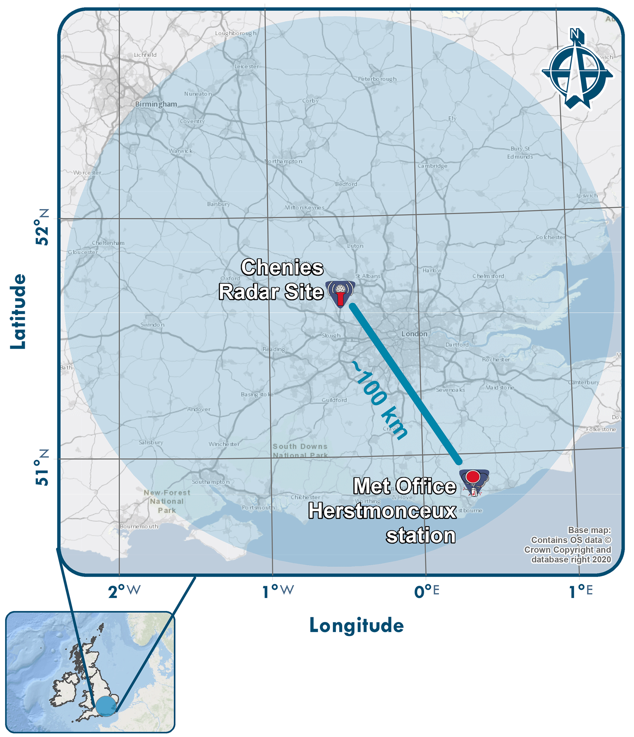
Figure 1Location and coverage (on short pulse, SP, mode) of the Chenies weather radar and location of the Herstmonceux radiosonde station. Source: base map contains OS data. ©Crown copyright and Crown database right, 2020.
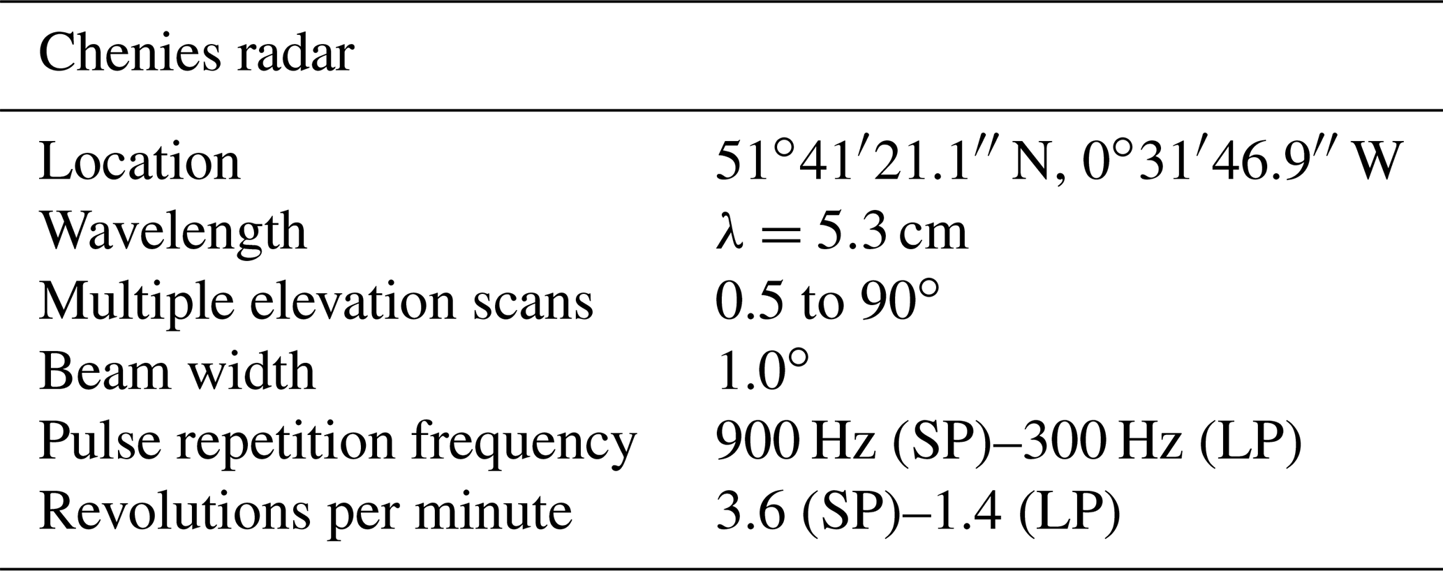
The Chenies C-band operational weather radar, located in southeast England, was selected for this work. It was one of the first UKMO radars upgraded with polarimetric capabilities (Norman et al., 2014). The radar transmits both horizontally and vertically polarised electromagnetic waves simultaneously and receives co-polar signals at the same polarisation as that of the transmitted wave, generating measurements such as ZH, ZDR, ρHV and ΦDP. Radial velocity (V) measurements of the observed precipitation targets are also available; LDR measurements are also produced for the lowest elevation scan (Met Office, 2013). The volume radar scanning strategy generates the following products:
-
A total of 5 PPI scans sampled on long pulse (LP) mode (pulse length is equal to 2000 µs; range covered is equal to 250 km) at 0.5, 1, 2, 3 and 4∘ elevation angles, with a 600 m gate resolution every 5 min.
-
A total of 5 PPI scans sampled on short pulse (SP) mode (pulse length is equal to 500 µs; range covered is equal to 115 km) at 1, 2, 4, 6 and 9∘ elevation angles, every 10 min, with the same gate resolution as above.
-
A single SP PPI scan at vertical incidence (range covered is equal to 12 km) every 10 min, with 75 m gate resolution.
-
A single PPI scan with LDR measurements every 5 min at the lowest elevation (0.5∘).
The location and other radar characteristics are provided in Table 1 and Fig. 1.
Polarimetric scans related to precipitation events throughout 2018 were analysed for the design and evaluation of the algorithm. To reduce the probability of ground clutter contamination and beam spreading effects, only SP scans from the 4, 6, 9 and 90∘ elevations angles were retained for further processing. Then, a pre-processing of the raw radar data is carried out to discard non-meteorological echoes and construct the profiles of polarimetric variables as follows:
-
For the 4, 6 and 9∘ elevation scans, remnant clutter and anomalous propagation echoes were removed using the algorithm proposed by Rico-Ramirez and Cluckie (2008), specifically calibrated with data from this radar. Then, following the procedure suggested by Ryzhkov et al. (2016), we generated QVPs of ZH, ZDR, ρHV and ΦDP measurements. The procedure suggests the azimuthal averaging of the polarimetric measurements at high-elevation scans (10–30∘), but such elevation angles were not available on our data sets; hence, we used the highest elevation angles available to generate the QVPs. Although it is possible to produce time-averaged QVPs to avoid local storm effects, we decided to keep the original time resolution of the QVPs; therefore, we produced one QVP for each PPI scan. Details on the construction of the QVPs are provided in Sect. 6.
-
For the scans taken at vertical incidence, the data related to the first kilometre above ground level (a.g.l.) are not usable due to some inherent radar limitations, e.g. the de-ionisation time of the transmit–receive (TR) cell (Timothy Darlington, Met Office, personal communication, 2019) or clutter contamination. After discarding the data below this height, an azimuthal averaging of the polarimetric and radial velocity data collected at vertical incidence was performed, generating VPs of ZH, ZDR, ρHV, ΦDP and V. For the analysed radar data sets, the spectral width variable was not available. We also define a new variable, the radial velocity gradient (gradV), computed using the gradient of the 90∘ radial velocity profile (note that ). This new variable accentuates the profile extremes related to the change in the hydrometeor fall velocities from ice or snow to rain. The gradient of V is computed using first-order central differences in the interior points and first-order forward or backwards differences at the boundaries; for an in-depth description of numerical differentiation and finite-differences methods, see Moin (2010).
Regarding the attenuation corrections needed for ZH and ZDR, for most of the scans used in this work (especially 90 and 9∘ elevation scans) we observed that rain attenuation was relatively small after analysing the total differential phase shift. Furthermore, the ML height is essential for implementing rain attenuation correction algorithms. Hence, no attempt was made to correct for attenuation.
Based on the constructed VPs and QVPs, a total of 94 rainfall events, with visible signatures of the melting layer on ZH or ρHV, were selected, i.e. an enhancement up to 30 dBZ on ZH or ρHV constantly decreasing below 0.90. Also, from the total number of rain events, only 25 events observed by the radar showed a suitable temporal matching with the data collected by the radiosondes, i.e. the difference in time between radar and radiosonde measurements do not exceed 2 h. This time window was set to minimise the impact of the variability of the height of the ML.
The VPs and QVPs of the polarimetric measurements are displayed in height versus time plots. This enables the visualisation of the temporal evolution of the polarimetric radar signatures in the melting layer. Figure 2 depicts a stratiform rainfall event recorded between 9 and 10 April 2018 using VPs and QVPs (9∘ elevation angle). It can be seen that every radar variable exhibits distinctive features that provide unique information for the identification of the melting layer on both VPs and QVPs; e.g. Fig. 2a–b and c–d exhibit regions of enhanced values of ZH (BB) and ZDR, respectively, that are visible just below 2 km in height. Concurrently, Fig. 2e–f and g–h show that ρHV and ΦDP are sensitive to the phase and shape of hydrometeors, while Fig. 2i shows that the fall velocities of snow particles are lower compared to rain particles, which is an important feature that can be used to detect the ML. Figure 2j shows the gradient of the radial velocity (gradV) generated from 90∘ elevation scans, where the BB enhancement is clearly visible at 2 km in height, and it is related to the increase in the fall velocities of the hydrometeors. The different BB signatures expected in the melting layer on the QVPs and VPs are explained next.
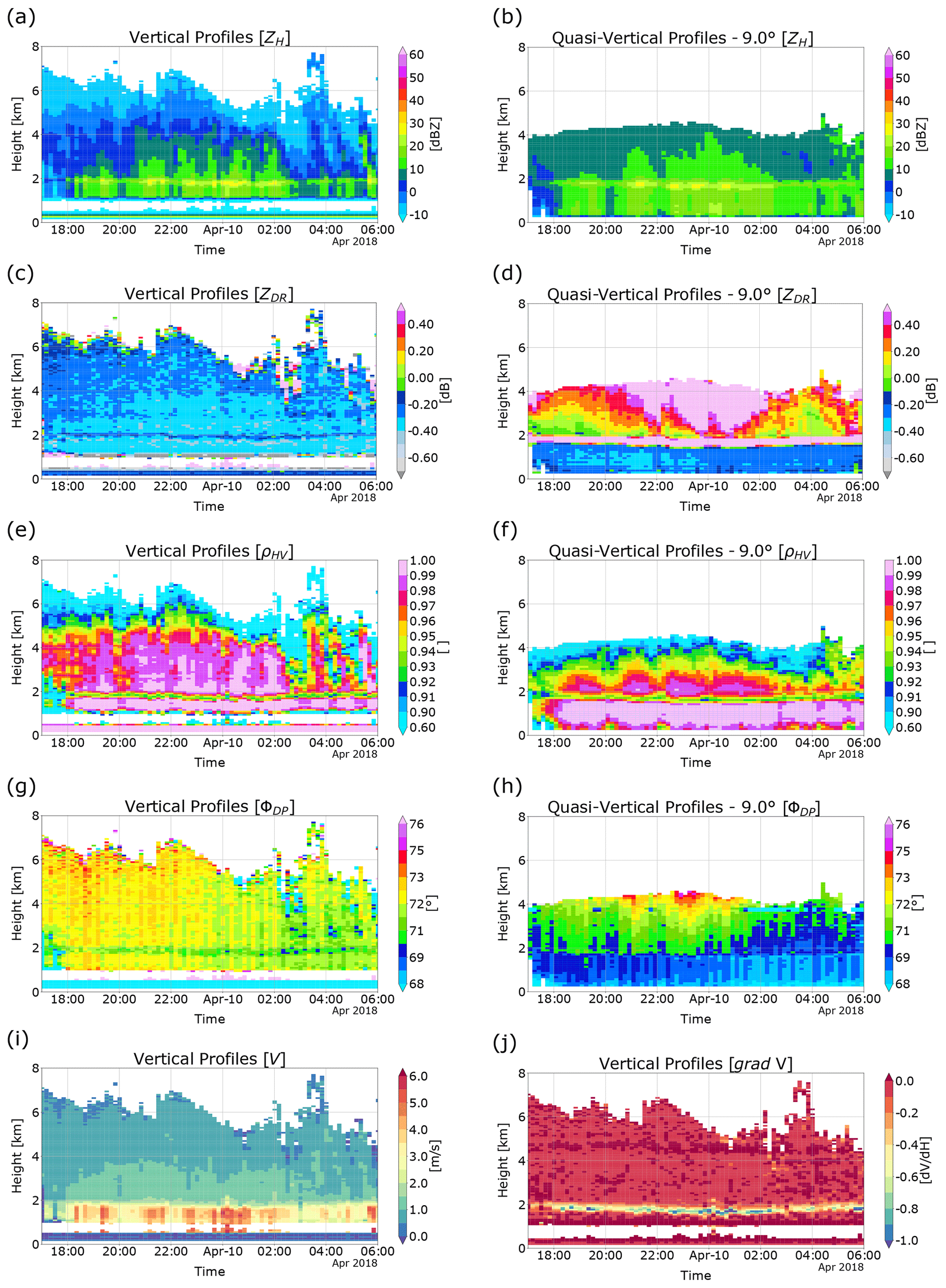
Figure 2Height versus time plots of ZH (a–b), ZDR (c–d), ρHV (e–f) and ΦDP (g–h), generated from VPs (left) and QVPs (right) for a precipitation event recorded by a weather radar located at Chenies, UK. Also, panel (i) portrays the radial (vertical) velocity V of hydrometeors, whilst panel (j) shows a plot of the profiles based on the gradient of V measurements .

Figure 3Normalised version of VPs and QVPs generated from polarimetric scans recorded at different elevation angles, related to a stratiform-type rain event. The 0 ∘C wet-bulb height is shown with the dashed–dotted line.
For comparison purposes, Fig. 3 shows normalised versions of VPs and QVPs (scaling each profile into the range [0, 1]) taken from the stratiform event presented in Fig. 2; also, the height of the 0 ∘C wet-bulb isotherm is shown. The normalisation process intensifies the signatures of the melting layer. Note that the QVPs provide information below 1 km; this is important for the analysis of showers or events with ML at relatively low altitude.
Given that the main objective of this work is to detect the melting layer boundaries based on the geometric features of the polarimetric profiles, herein, we will try to explain how the melting layer shapes the structure of the radar profiles. Figure 3 shows the presence of enhancements on the polarimetric profiles related to the variation in the phase and concentration of the hydrometeors. Taking the 0 ∘C wet-bulb height as a reference (just below 2 km in altitude), it is feasible to associate the upper boundaries of these enhancements to the ML. These enhancements are not necessarily at the same height in all polarimetric variables, but this has to do with the backscattering properties of the melting particles and their relationship with the measured variable. Also, it is important to highlight that the methods used in the construction of the profiles play a key role in the location of the peaks, i.e. both VPs and QVPs result from an azimuthal averaging of the rays, representing an average structure of the storm that helps to enhance the BB signature. So, the BB peaks in the VPs and QVPs in all radar measurements differ from the instantaneous profiles observed at individual slant ranges; this will be discussed in Sect. 6.
The reflectivity (ZH) represents the power backscattered by precipitation particles, thus providing information about the concentration, size and phase of the hydrometeors (Hong and Gourley, 2015). In Fig. 2a and b, it can be seen that the values of ZH on both QVPs and VPs show similar intensities. Also, the well-known BB effect on ZH is visible on both profiles (around 1.7 km). The BB is caused by the increase in the dielectric constant of melting particles, by the change in size from large melting snowflakes to raindrops and by the increase in the fall speed of the hydrometeors that reduce the particle concentration (Fabry, 2015). The BB is easily observed in stratiform events; however, it is difficult to set the melting layer boundaries based only on ZH; e.g. in Fig. 3a, the top of the BB is not easy to discern. Moreover, the profiles of ZH do not show the BB feature in convective events; therefore, the estimation of ML for convective events, based only on ZH, is not feasible.
The differential reflectivity (ZDR) represents the ratio between horizontal and vertical reflectivity values (), and it is related to the orientation, shape and size of the hydrometeors (Islam and Rico-Ramirez, 2014); therefore, ZDR measurements for QVPs and VPs may describe different features of the particles as the elevation angle varies. For both QVPs and VPs, ZDR profiles show similar behaviour in stratiform events. Figure 3b shows that ZDR exhibit mean small slope changes on the rain medium (below 1.2 km), but there is a noticeable peak associated with the melting layer on both VPs and QVPs, and although there is a difference in the peak height between both types of profiles, the top and bottom boundaries are at similar heights, especially for the QVPs. Brandes and Ikeda (2004) and Ryzhkov et al. (2016) showed that the presence of melting, randomly oriented ice particles within the melting layer and the mixing of hydrometeors produce the peaks in ZDR in stratiform events. However, for profiles related to convective events (not shown), the VPs sometimes exhibit an inverse peak exactly above the rain medium and then generate a noisy, random pattern on the melting layer that makes the estimation of the ML more difficult when using VPs of ZDR. Finally, the most significant difference for this variable can be seen in Fig. 2c and d, where the values of ZDR for VPs and QVPs differ from each other, especially in the melting layer and above. It is also important to highlight that ZDR provides valuable information for QPE. However, it usually shows a bias that must be corrected; e.g. in Fig. 2c there is a bias in ZDR ( dB) as we expect near-to-zero values for ZDR in the rain region for vertically pointing measurements, as raindrops are symmetrical on average when observed from underneath (Gorgucci et al., 1999). A subsequent analysis of birdbath scans in light rain through the whole data set confirmed a persistent offset in ZDR. This reaffirms the importance of the detection of the melting layer boundaries, as it helps to set limits for the implementation of a ZDR calibration algorithm.
The correlation coefficient (ρHV) measures the correlation between the backscatter amplitudes at vertical and horizontal polarisations. It is sensitive to the distribution of particle sizes and shapes and, hence, sensitive to the hydrometeors phase, becoming a valuable hydrometeor classifier for identifying non-meteorological echoes (Islam and Rico-Ramirez, 2014). Additionally, ρHV is a reliable indicator of the quality of the radar data as, in the rain medium, the correlation is close to 1, becoming an indicator of the quality of the polarimetric radar measurements (Kumjian, 2013a). Figure 2e and f show that ρHV is close to one within the rain region, which confirms the high quality of this radar data set. Figure 3c shows that the melting layer causes a similar response on ρHV as in ZH and ZDR, but in the opposite direction, resulting in a depression on the profiles starting at 1.4–1.5 km in height for QVPs and VPs, respectively. This depression results from the shift between high values of ρHV, related to raindrops and ice crystals and lower values triggered by the variety of shapes and axis ratios of the hydrometeors (Kumjian, 2013b). The behaviour of ρHV is similar on both VPs and QVPs from 9∘ elevation for stratiform or convective events, where the major difference lies in the depth of the depressions. This may be caused by the resolution and elevation angle of the original scans. On the other hand, the QVPs constructed from lower elevation angles, i.e. 4 and 6∘, exhibit less pronounced peaks related to the melting layer, and a pronounced decrease in ρHV above the BB that can make it difficult to identify the ML.
As can be seen in Figs. 2g–h and 3d, the signatures of the melting layer on the differential propagation phase (ΦDP) are, to a certain degree, ambiguous in our data sets, especially on the QVPs. ΦDP represents the difference between the phase of the radar signal at horizontal and vertical polarisation, providing valuable information about the shape and concentration of the hydrometeors (Islam and Rico-Ramirez, 2014). Hence, the peaks on this type of profile may be related to a greater concentration of particles due to the presence of the melting layer or the dendritic growth layer (DGL), as previously explored by Griffin et al. (2018), Kaltenboeck and Ryzhkov (2017) and Ryzhkov et al. (2016). Figure 3d shows that the QVPs of ΦDP from 9∘ elevation exhibit a small peak at 1.7 km in height related to the melting layer, but it is not as pronounced as with the other polarimetric variables, although there are significant peaks aloft (between 2.8 and 3.8 km) that may represent particle (ice or snowflakes) alignment on the DGL, as suggested by Kaltenboeck and Ryzhkov (2017), while lower elevation angles do not show strong signatures on the melting layer or the DGL. In contrast, for 90∘ elevation scans, there is a well-defined depression in ΦDP related to melting and particle growth (Brandes and Ikeda, 2004) at 1.8 km in height that closely matches the height of the BB; regarding the signatures of the DGL on the VPs, due to the noisiness of the profile above the ML, it is difficult to determine if these peaks are related to the DGL.
Figures 2i and 3e show the profiles related to the radial (vertical) velocities (V) and the signatures of the melting layer on this variable. It can be seen that the fall velocity of the hydrometeors is relatively constant and close to zero above the ML, which is related to the fall velocity of ice and snow particles; then, there is a sharp increase in the fall velocity of the precipitation particles in the melting layer that becomes constant again in the rain region. However, it is challenging to incorporate the velocity profile into the ML detection because its features are not easy to identify using an automated peak search algorithm. Conversely, the VP of the radial (vertical) velocity gradient (gradV), shown in Figs. 2j and 3e (dotted line), exhibits a BB enhancement and peak similar to the rest of polarimetric variables, where the upper and lower curvatures of the peak match the top and bottom extents of the melting layer.
The melting level algorithm (MLA) automatically detects the ML, using either QVPs or VPs, under the premise that the peaks on each polarimetric profile and their curvatures are related to the melting layer. The MLA is based on the procedure proposed by Wolfensberger et al. (2016) that combines ZH and ρHV to create a new profile with enhanced melting layer features. However, Fig. 3 shows that there are additional variables, such as gradV, that may improve the identification of the ML. Therefore, we propose an algorithm that combines all the various radar signatures to estimate the melting layer boundaries. A subsequent analysis of the outputs of the algorithm, in combination with radiosonde data, determines the combination of radar signatures that is the best predictor of the ML. Some considerations are made for its design; for example, to minimise the effect of beam broadening, the analysis is constrained to a height of 5 km (for 9∘ scans, the height of the centre of the beam is similar to 30 km in range). Also, as shown in Fig. 3, some profiles become noisy above the ML or contain spurious echoes aloft, making it necessary to set an initial upper extent for the algorithm to work. The MLA is divided into two parts. The first part determines if the profile contains elements for detecting the melting layer based on the combination of two profiles and setting an upper limit for its implementation. The second part estimates the ML based on a combination of the polarimetric profiles and their features. The algorithm uses either QVPs or VPs, but we avoid combining both profiles, as VPs might not be available in other weather radar networks. A flow chart that illustrates the MLA steps is shown in Fig. 4 and described below.
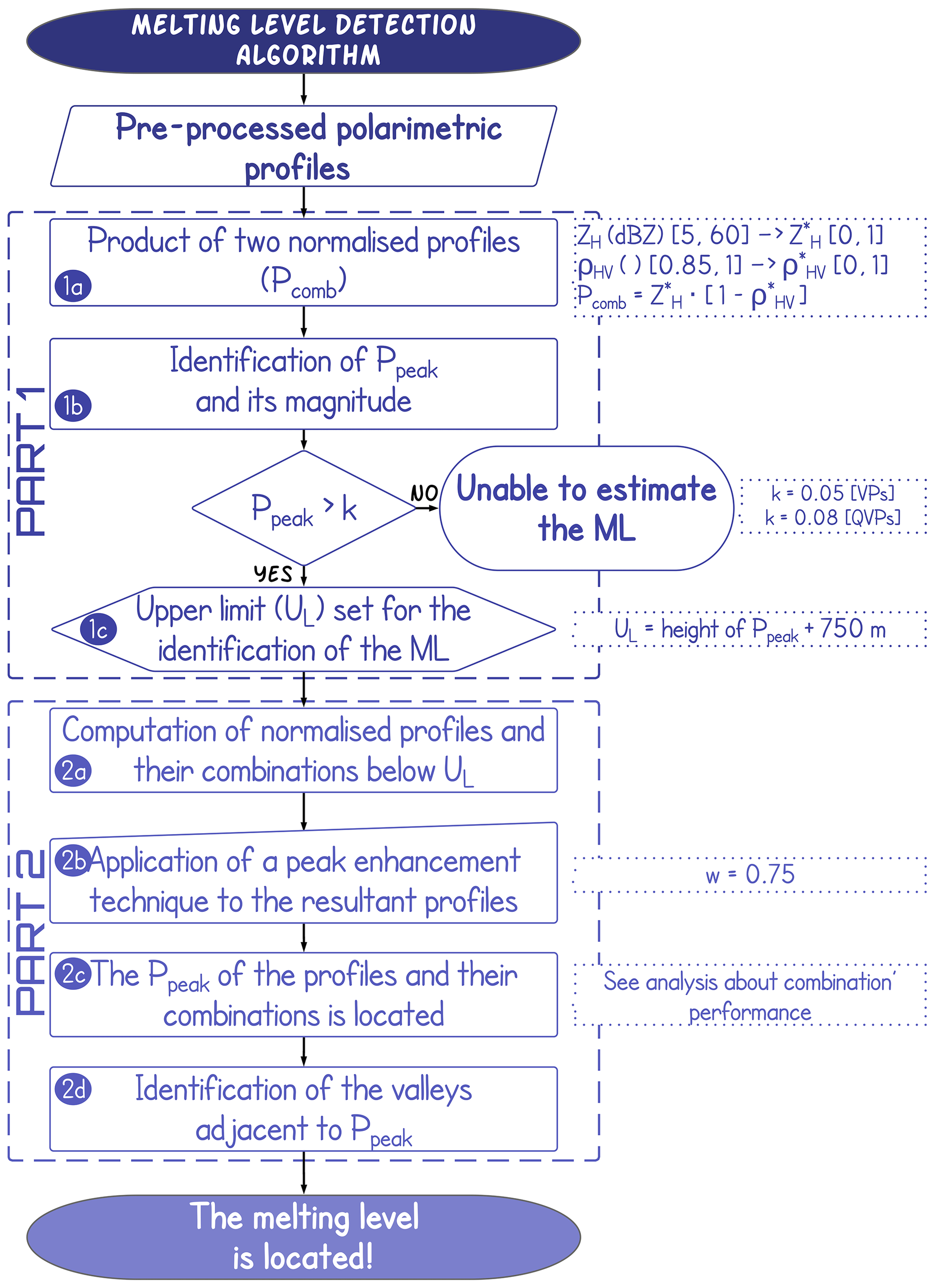
Table 2Possible combinations of polarimetric variables for VPs and QVPs used for the ML detection.
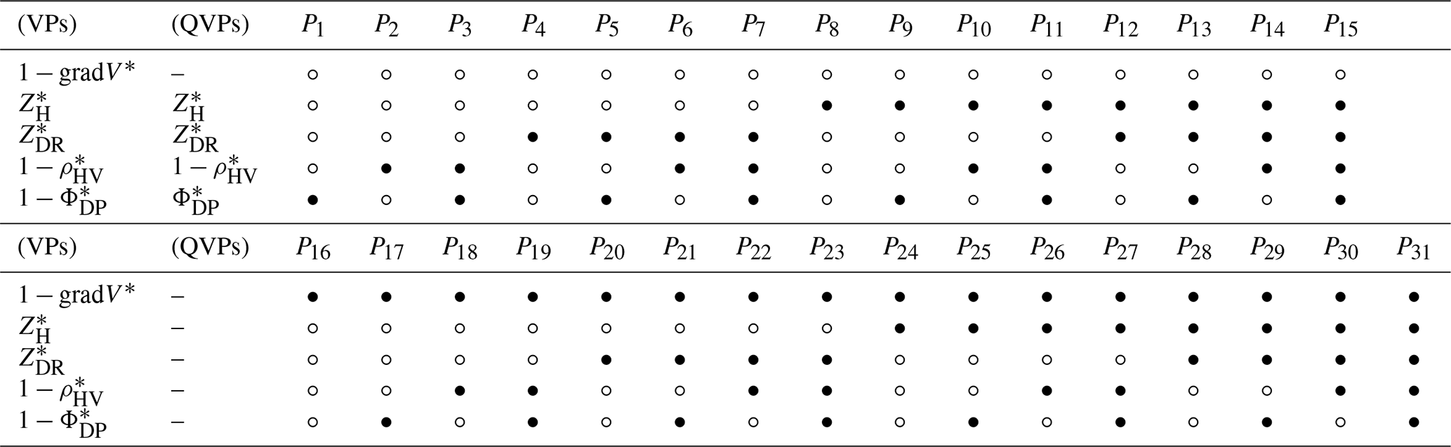
Note: The asterisk (∗) refers to the normalised version of the variables.
- 1.
Part 1
The first part of the MLA identifies profiles that are likely to contain signatures related to the melting layer and sets an upper limit in the profiles to use all the available variables.
- 1a.
The algorithm takes advantage of the distinctive signatures on the profiles of ZH and ρHV, on both VPs and QVPs, to perform an initial identification of rain echoes. These two profiles are normalised and combined into a single profile (Pcomb), as suggested by Wolfensberger et al. (2016), but using different thresholds for ZH and ρHV related to drizzle, heavy rain, snow and ice (Kumjian, 2013a; Fabry, 2015). Hence, values of ZH, between 5 and 60 dBZ, and ρHV, between 0.85 and 1, are normalised to 0 and 1 as follows: and . Values outside these intervals are fixed to 0 and 1, correspondingly. The normalisation is carried out using the min–max normalisation procedure. Then, the normalised profiles are combined using the complement of ρHV to enhance the peaks present in the profiles as follows:
Note that the asterisk (∗) refers to a normalised variable.
The profile Pcomb is likely to show an enhanced peak if potential melting layer signatures were present in the profiles of ZH and ρHV.
- 1b.
The MLA locates the peaks on the profile Pcomb by comparing neighbouring values. A peak is a sample for which the direct neighbours have smaller magnitudes. Inversely, the valleys (or boundaries of the peaks) within the profile can also be detected using a similar rationale. As several peaks can be present in the profile, the peak with the higher magnitude (i.e. the horizontal distance between the peak and the origin) is set as Ppeak. Then, to identify profiles with a Ppeak strong enough to be related to potential melting layer signatures, a threshold, k, is set. If the magnitude of Ppeak is less than the threshold, k (set to 0.05 for VPs and 0.08 for QVPs), the MLA determines that the gradients are not strong enough to correspond to melting layer signatures, and therefore, the profile does not contain elements for detecting the ML. This step is illustrated in Fig. 5a, where the magnitude of Ppeak (∼0.14) is greater than the threshold, k. Further discussion on the value of this parameter is provided in Sects. 4.1 and 6.
- 1c.
If the magnitude of Ppeak is greater than k, an upper limit (UL) is set, taking the height of Ppeak and adding 750 m above. This value is selected as the melting layer thickness usually reaches values less than about 800 m (Fabry and Zawadzki, 1995); hence, 750 m is sufficient for refining the search of the ML. Figure 5a illustrates this step, where 750 m are added to the height of Ppeak (∼1.51 km) to set an upper limit (∼2.26 km).
- 1a.
- 2.
Part 2
In the second part of the algorithm, we incorporate the rest of the polarimetric variables to analyse their capability for refining the detection of the melting layer boundaries and determining the combination that better detects the ML.
- 2a.
In this step, the profiles of all the radar variables are cut below UL. Then, and considering that and were already normalised in step 1a, the other variables are also normalised but use the minimum and maximum values in each profile as thresholds. To incorporate all the variables into the algorithm, the complement of the variables is used when appropriate. This is made to generate profiles with analogue peaks that enhance the footprints of the melting layer when combined with other variables. Equations (2) and (3), respectively, are derived based on the patterns observed in VPs and QVPs. These equations vary according to the combination of the variables presented in Table 2.
where i depends on the combination of the variables used according to Table 2.
The algorithm computes all the possible combinations of the profiles to analyse the influence of each variable by, in this case, generating 31 different profiles if using VPs and 15 profiles when using QVPs.
- 2b.
The profiles () generated in the previous step will very likely show a peak related to the melting layer. The next step in the MLA is to apply a peak enhancement technique to refine the boundaries of this peak. This can be done using the following equation:
where Pi is the enhanced profile, is the profile given by Eqs. (2) or (3), w is a weighting factor, and is the second derivative of . The optimum choice of the parameter w depends upon the signal-to-noise ratio and the desirable sharpening extent. Table 2 lists the enhanced profiles produced by combining different polarimetric profiles, and Fig. 5b shows the enhancement of the peak and valleys. Details on the value of the parameter w are presented in Sects. 4.1 and 6.
- 2c.
For each profile Pi, the maximum enhancement in the BB has a magnitude given by Ppeak and computed as in step 1b. Then the parameter k is used to discard profiles with peaks not related to the melting layer (k=0.05 for VPs; k=0.08 for QVPs).
- 2d.
The top and bottom boundaries of the BB enhancement in Pi can be placed by searching the inverse peaks (valleys) directly above and below Ppeak. Finally, the algorithm allocates these points as being the boundaries of the melting layer. This step is shown in Fig. 5c, where the selected profile P26 is highlighted. The top valley of Pi is set as the estimated height of the ML (MLTop).
- 2a.
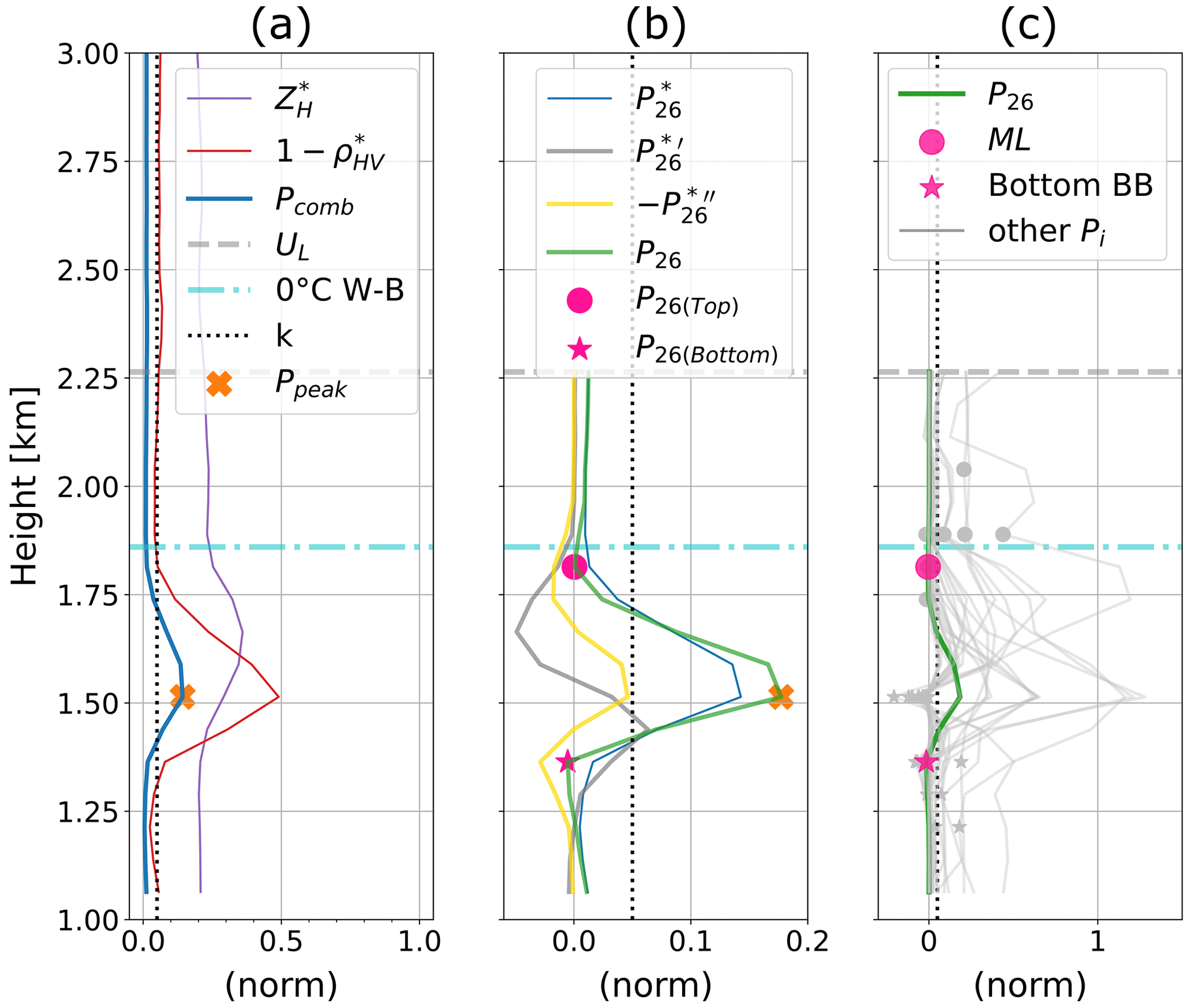
As can be seen in Fig. 5a, the combination of and produces a profile with a peak (Ppeak) that is useful for detecting the presence of the melting layer. An adequate choice of the magnitude of the parameter (k) is important to discard profiles with a Ppeak that is not strong enough to be related to the melting layer. However, additional variables can be used (see Eqs. 2 and 3) to refine the detection of the ML. The upper limit (UL) allows the use of other variables that otherwise could not be part of the algorithm due to noisiness or spurious echoes present at the top of the profiles. Figure 5b shows the importance of the refinement of the profile, e.g. the profile combination ) (blue line) has a peak related to the melting layer, and the valley located at the top of this peak is close to the ML, but it is difficult for a peak detection algorithm to detect its height, as it is not as pronounced as required. The use of the first derivative of the profile, i.e. (grey line), is not helpful, as the peaks are not close to the ML. The profile P26 (green line) results from the implementation of Eq. (4), where a value of w equal to 0.75 enhances the peak and its valleys enough for the algorithm to detect their boundaries. A proper choice of the parameter w depends on the desired weight to the original profile rather than its second derivative. The impact of the parameters k and w on the algorithm is discussed in the following section.
4.1 Implementation of the ML algorithm
As described before, the MLA performs a pre-classification of profiles likely to contain melting layer signatures. Some tests were carried out by replacing with other variables (e.g. ZDR or ) to identify improvements in the pre-classification. From Fig. 3b, it is clear that the QVPs of ZDR exhibit a pronounced peak related to the melting layer, even for low elevation angles, but unfortunately, ZDR is not calibrated, and the thresholds for normalising this variable may vary depending on the elevation angle. On the other hand, replacing with the profile for the VPs could improve the pre-classification, but this may restrict the implementation of the algorithm, i.e. it would be only applicable if vertical velocity profiles are available. Although we observed some improvements using these variables in the first part of the MLA, especially for rain showers, we wanted to keep this part as simple and robust as possible to enable the reproducibility of the algorithm. Hence, we used the combination of and ρHV for part 1 of the algorithm, as initially proposed by Wolfensberger et al. (2016).
On the other hand, the algorithm relies on the parameters k and w, as shown in Fig. 5a and b. These parameters can be adjusted according to the radar data sets, e.g. the parameter k can be affected by the quality of ρHV. In our data sets, and after the removal of non-meteorological echoes, ρHV exhibits values close to 0.85 in the melting layer on both QVPs and VPs, but this may vary depending on the type of radar, scanning strategy and quality of the data sets. We set k equal to 0.05 for VPs and k equal to 0.08 for QVPs empirically, and these values allow the algorithm to discard enhancements in the profile not related to the melting layer. Moreover, several tests were carried out using time-averaged QVPs, resulting in smoother profiles, and this parameter was helpful for identifying profiles with melting layer signatures. On the other hand, Eq. (4) is applied to the profiles to enhance the BB peak and the top and bottom boundaries (i.e. valleys) within the profile, thus refining the detection of the ML. This equation combines the original profile with its second derivative, weighted with the parameter w. As shown in Fig. 5b, the second derivative of the profile (yellow line) exhibits deeper peaks, but its top boundary is still far from the measured ML. After several trials, we set w equal to 0.75, as this value enhances the peaks of the original profile without compromising the match of the top boundary and improving the ML detection. Likewise, this parameter can be adjusted depending on the radar data sets, e.g. profiles that exhibit smoother peaks due to the nature of its construction process and the resolution of the original scans, or profiles with vertical resolution too coarse can be adjusted with the parameter w for a better algorithm performance.
5.1 VP and QVP comparison
Both VPs and QVPs proved to be an efficient way of monitoring the temporal evolution of the melting layer, but the elevation angle used to build the QVPs affects each radar variable in different ways, as described in Sect. 3 and shown in Figs. 2 and 3. Hence, to support the performance and outputs of the algorithm, we assessed the consistency between the ZH profiles constructed from different elevation angles, as this is the variable less prone to significant variations due to the elevation angle. For the rest of the variables, it is not possible to compare QVPs as their characteristics vary with the elevation angle used to build the QVPs.
To carry out this analysis, we manually classified the rain events recorded by the radar according to the recommendations of Fabry and Zawadzki (1995) and Rico-Ramirez et al. (2007). From a total of 94 rainfall events, 68 events were classified as stratiform. This category includes low-level rain and rain with BB, as they showed the well-known enhancement of reflectivity observed within the melting layer or look-alike drizzle events below the 0 ∘C. On the other hand, 26 events recorded mainly during the summer met the characteristics of showers, i.e. indistinguishable signatures of the melting layer in the ZH profiles, in which higher values of reflectivity are present; the latter is the type of precipitation less common in the UK (Collier, 2003). The comparison between VPs and QVPs takes into account the timestamp and spatial resolution of the profiles. The Pearson correlation coefficient (r) is computed to analyse the consistency between the VPs and QVPs. The results for stratiform and convective events are shown in Figs. 6 and 7, respectively.

Figure 6Comparison of VPs and QVPs of ZH generated at two elevation angles for a collection of stratiform events. Counts indicate the number of points in the hexagon.
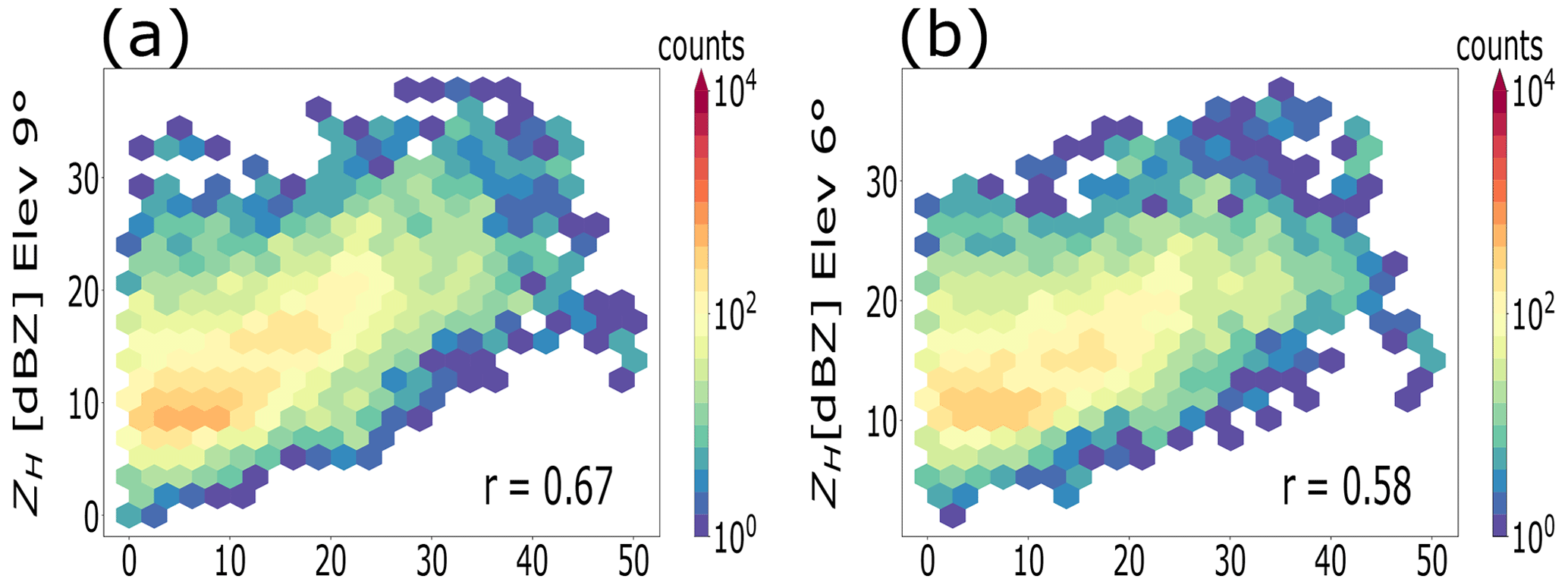
Figure 7As in Fig. 6 but for a collection of convective events. Counts indicate the number of points in the hexagon.
Figure 6 shows that reflectivity values related to light and moderate rain rates (expected on stratiform-type events) are similarly depicted on both VPs and QVPs. However, the agreement diminishes when decreasing the elevation angle, mainly because higher values of ZH do not always match their pairs as the elevation decrease. This could be explained by the averaging process carried out in the construction process of the profiles, as the radar resolution volume increases with distance. On the other hand, Fig. 7 shows a more scattered distribution of ZH for shower-type events in which higher values of ZH (related to moderate to heavy rain rates) are present. Again, the correlation decreases for lower elevation angles, and it can be seen that there are mismatches for cells with higher values of reflectivity. This can be related to local storm effects and spatially nonuniform convective elements present in the QVPs, as explored by Ryzhkov et al. (2016). It is worth mentioning that QVPs constructed from lower elevation angles were also assessed (results not shown), but similar behaviour was observed, e.g. correlation decreases even further. Also, a similar analysis was carried out using other polarimetric variables. However, the results were not consistent as only ZH describes similar properties of the precipitation measurements taken at these elevation angles.
5.2 ML detection from VPs
The MLA outputs were analysed to find the combination of VPs that better detects the ML. These outputs are compared against 0 ∘C wet-bulb isotherms over 1 year of rainfall events. Since soundings are released twice daily, the radiosonde data are extended at several time steps to create short time windows and enable a comprehensive comparison with the radar data. Performance metrics (Pearson correlation coefficient – r; mean absolute error – MAE; root mean square error – RMSE) between the height of the 0 ∘C wet-bulb isotherm and the estimated ML are computed. Figure 8 shows the results for a 60 min window, i.e. the height of the 0 ∘C wet-bulb isotherm is assumed constant 30 min before and after the timestamp of the radiosonde.
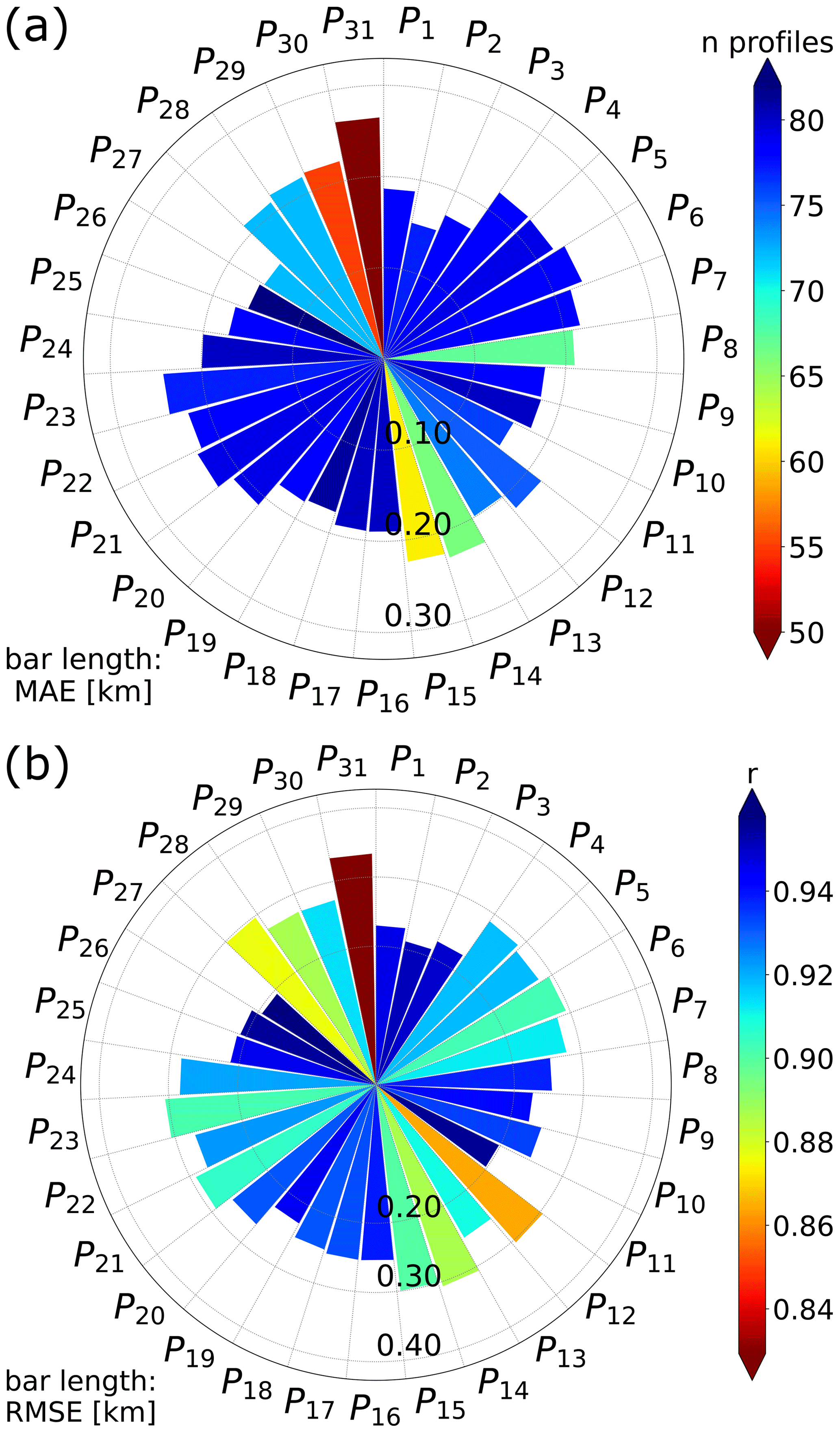
Figure 8Errors in the ML detection for VPs using a ±30 min window. In panel (a), the bar length represents the MAE (in kilometres), and colour represents the number of vertical profiles with strong signatures detected by every polarimetric combination; in panel (b), the bar length represents the RMSE (in kilometres) for every polarimetric combination, and colour represents the Pearson correlation coefficient.
Figure 8 shows the capabilities of all polarimetric variables for the detection of the ML. In Fig. 8a, the variable n profiles is an indicator of the number of profiles that, according to the algorithm, contain peaks strong enough to be related to the melting layer. This variable can only be validated by a visual inspection of the algorithm outputs, as some variables may incorrectly classify some peaks as being melting layer related. Overall, Fig. 8 shows that the combinations that include , or improve the accuracy of the MLA, e.g. P9, P11 or P26, as the correlation, and the errors are relatively low for these combinations. After a visual assessment of the performance of each combination and supported by the statistics computed above, we determine that the profile combination is the best predictor of the ML. Then, several time windows are set to assess the accuracy of the MLA over 1 year of radar data, as shown in Fig. 9. This analysis confirms the good performance of the combination P26 on the ML detection, even when increasing the time window, as the RMSE and MAE are close to 200 m and r equals 0.95. Another indicator taken into account in the visual inspection of the algorithm output was the detection of the melting layer bottom and its steadiness regarding the ML. Examples of the detection of the melting layer for stratiform and convective events using the profile P26 are shown in Fig. 10. Figure 10a and b show the output of the MLA using the combination P26 in both stratiform or convective events. The algorithm shows a good performance, especially for stratiform events where the ML height and the rain zone are accurately defined. For the convective event, the ML is correctly identified, although the bottom of the melting layer is not entirely detected. This is a drawback when using the algorithm based on VPs and highlights the problems when low-altitude melting layers are present.
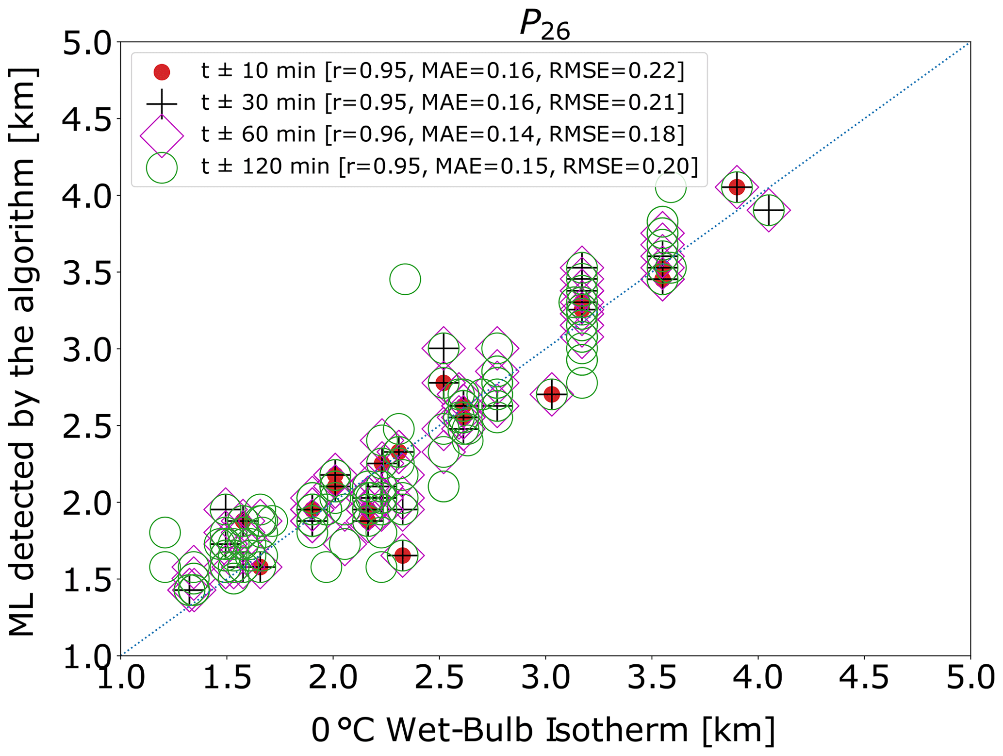
Figure 9Heights of the 0 ∘C wet-bulb isotherm versus ML detected by the algorithm using the combination P26 for several time windows. The 1 : 1 line is shown in blue. MAE and RMSE are shown in kilometres.
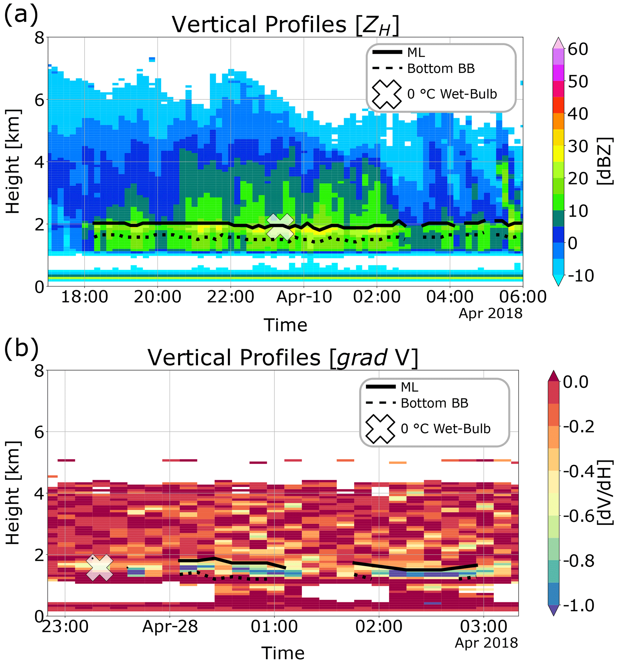
Figure 10Comparison of the MLA outputs based on the variable P26 at 90∘ elevation angle for two different rain events. Panel (a) shows the detection of the melting layer for a stratiform event displayed over a height versus time plot of ZH, and panel (b) shows the performance for a convective event displayed over a height versus time plot of gradV.
5.3 ML detection from QVP
The MLA is applied to QVPs generated from scans at three different elevation angles (4, 6 and 9∘). After several trials on the parameters k and w in the algorithm implementation, only the highest elevation produced satisfactory ML estimation results. The explanation of this has its foundation in Fig. 3c, where QVPs from lower elevation angles display shapes that complicate the implementation of the algorithm. For instance, the profile of ρHV exhibits a peak related to the ML, but above this peak, the values of ρHV decrease sharply, while the profile of ZH exhibits smoother peaks, and when the normalisation process is carried out, the parameter k cannot correctly filter gradients related to the ML. Thus, after several trials, and supported by the analysis presented in Sect. 5.1, we decided not to use the lower elevation angles (4 and 6∘). Using the same windows as in the VPs, we computed several performance metrics (r, MAE and RMSE) between the 0 ∘C wet-bulb isotherms and detected MLs. The performance of the algorithm using different profiles and a time window of 60 min (i.e. using radar profiles 30 min before and after the radiosonde timestamp) is shown in Fig. 11.
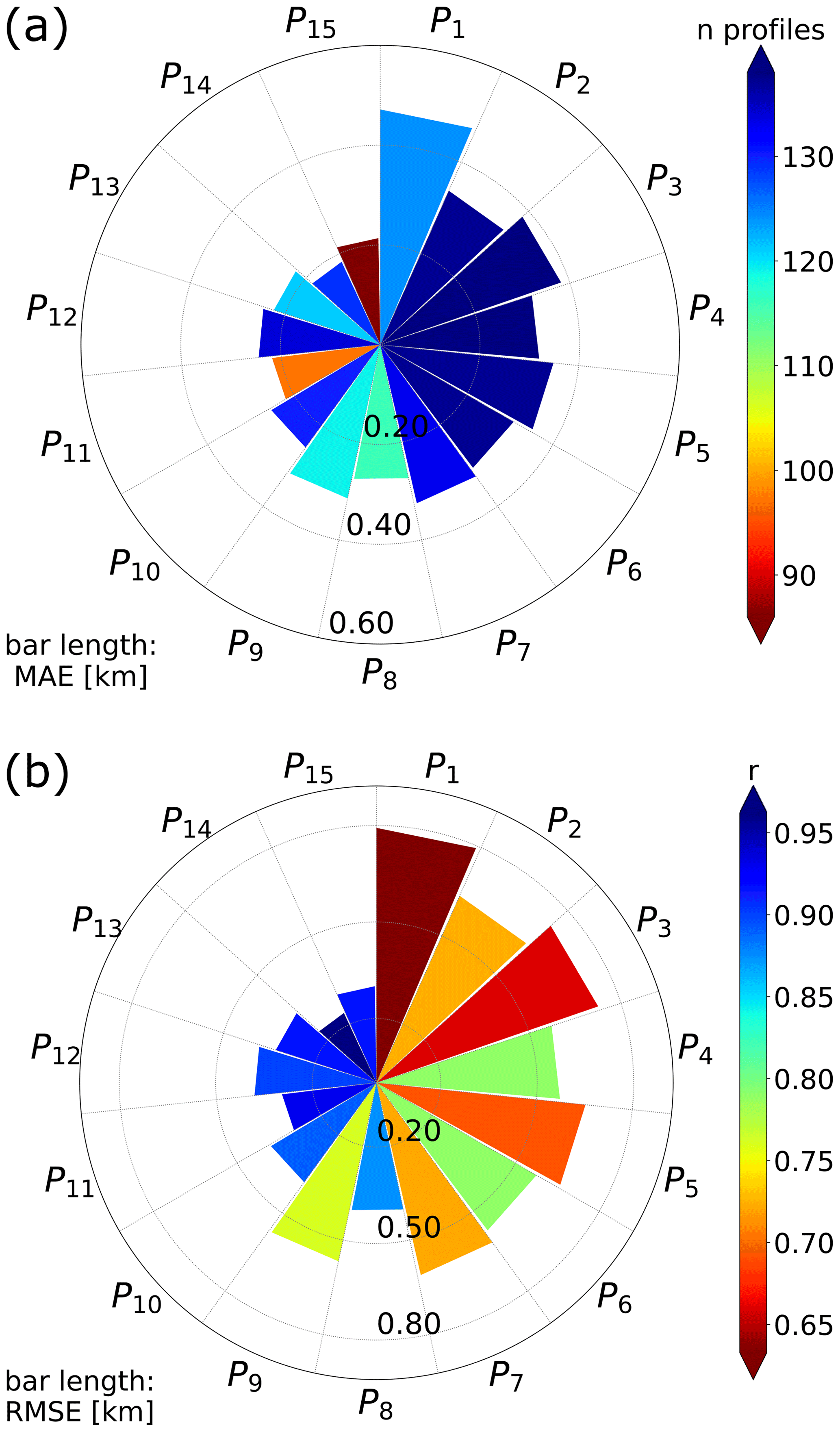
Figure 11Errors in the ML detection for QVPs using a ±30 min window. In panel (a), the bar length represents the MAE (in kilometres), and colour represents the number of QVPs with strong signatures detected by every polarimetric combination; in panel (b), the bar length represents the RMSE (in kilometres) for every polarimetric combination, and colour represents the Pearson correlation coefficient.
Figure 11a shows that the number of profiles covered by the time window is somewhat greater than the number of profiles covered in the implementation of the VPs. This is expected because the coverage area of the PPIs from where the QVPs were constructed is greater than the vertical scans. Overall, the four indicators in Fig. 11 stress the influence of ZH and ρHV in the estimation of the ML height and reveal that adding the combination to the analysis, i.e. P12, P14 or P15, improves the delimitation of the ML, given that these combinations exhibit high values of correlation (r), and the errors are below 250 m. Based on these results, and combined with a visual assessment of the outputs of the algorithm over 1 whole year of precipitation profiles, we concluded that the profile that combines , and (), i.e. P14 provides the best detection of the ML. The performance of the algorithm using this combination is shown in Fig. 12.

Figure 12Heights of the 0 ∘C wet-bulb isotherm versus ML estimated by the algorithm for several time windows using QVPs from 9∘ elevation scans. The 1 : 1 line is shown in blue. MAE and RMSE are given in kilometres.
Figure 12 shows that error and correlation coefficient decrease as the time interval increase. Given that the errors are close to 250 m for short time windows, this combination proves to be accurate for the ML detection, making allowance for the original resolution of the scans (600 m). A total of two examples of the outputs of the algorithm, using the profile P14, are shown in Fig. 13 for the same stratiform and convective events as in Sect. 5.2. The combination P14 shows that the ML is correctly detected, and the delineation of the rain region is well executed. For the convective event of Fig. 13b, the outputs of the algorithm are accurate for the ML estimation, although some gaps are present due to the filtering of profiles in the first part of the algorithm.
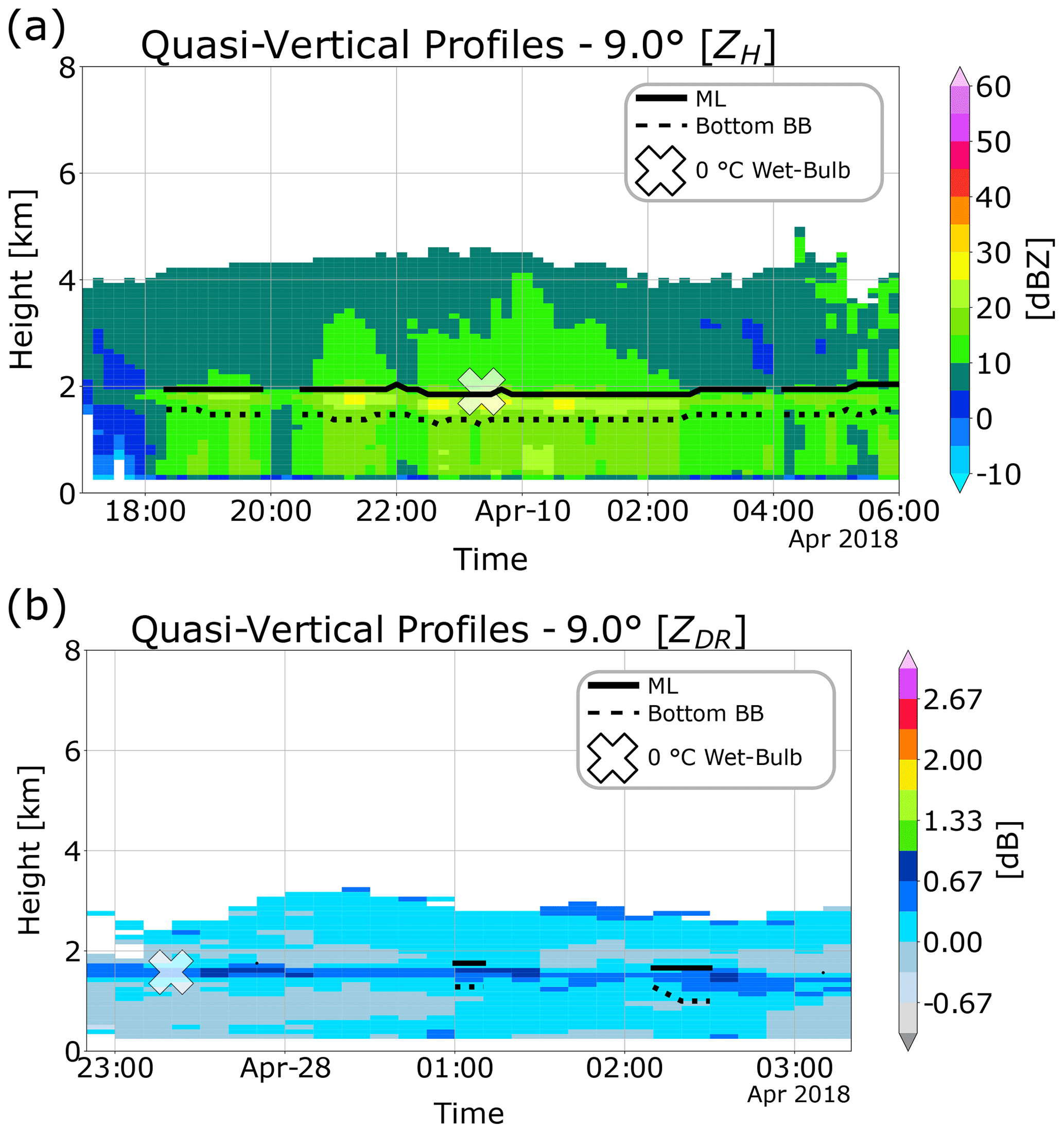
Figure 13Comparison of the MLA outputs based on the variable P10 for QVPs constructed from 9∘ elevation angle scans. Panel (a) shows the detection of the melting layer for a stratiform event displayed over a height versus time plot of ZH; panel (b) shows the performance for a convective event displayed over a height versus time plot of ZDR.
We constructed VPs and QVPs of polarimetric variables to explore precipitation events and their features. As shown in Fig. 2, both types of profiles display differences influenced by the scan elevation angle and the methods used to construct the profiles. Regarding the latter, there are several points worth discussing.
- i.
It is possible to generate time-averaged QVPs to smooth the effects related to local storm structures; the averaging process over the radar domain, combined with temporal averaging, reduces the signal noise, and it may help to discard profiles with signatures not related to the melting layer. However, the duration of the rain events and other factors raises a question about the correct time window length. After several attempts with different time windows, we observed that the signatures of the melting layer are often easier to discern in profiles related to stratiform events. However, for convective events, the main variables that detect the ML, e.g. ZDR or ρHV, are affected by the temporal averaging, blurring the melting layer signatures. Thus, we present examples of instantaneous QVPs; however, we kept this matter in mind for the MLA design.
- ii.
The spatial variation in the rain events is a limitation of both VPs and QVPs. The former captures the storm structure only directly above the radar location. Moreover, for the data sets used in this work, scans taken at 90∘ elevation present limitations when reading data on the first kilometre due to technical restrictions; this situation restrains the observation of rainfall features at relatively lower altitudes. On the other hand, the PPIs from where the QVPs are constructed may contain sectors with non-homogeneous echoes, e.g. a combination of mixed precipitation is possible at ranges far from the radar because the beam is considerably bigger. Moreover, at certain stages of the storm evolution, the radar echoes are insufficient to generate QVPs with clear signatures of the melting layer or even valid QVPs. This horizontal heterogeneity introduces uncertainty into the QVPs, as stated by Ryzhkov et al. (2016). These limitations on the generation of the QVPs require further investigation and are out of the scope of this work, since our main objective is to detect the melting layer signatures.
- iii.
Due to the averaging process on the construction of the profiles, the BB shape and height do not exactly match profiles found in previous studies, especially from profiles generated from measurements collected using vertical cross sections. For instance, Brandes and Ikeda (2004), in their Fig. 1, showed that the BB peak in ZH is higher in altitude compared to the BB peak in ZDR, whereas, in our Fig. 3a and b, the peaks are at similar heights due to the azimuthal averaging. Our data sets show similar signatures to those shown by Brandes and Ikeda (2004) (figures not shown) when the profiles are extracted from slant ranges. Although the BB peaks are not the same in our VPs (or QVPs) due to the azimuthal averaging, the BB boundaries are on average at similar altitudes and are, hence, not a major problem for implementing the MLA.
After this, we analysed the different signatures of the melting layer in the VPs and QVPs. We observed that ZH is a variable susceptible to the different types of precipitation on both VPs and QVPs, allowing the characterisation of the rain profiles, as previously explored by Fabry and Zawadzki (1995), Kitchen et al. (1994) and Klaassen (1988). Nevertheless, this also accentuates the trouble of detecting the ML based only on the reflectivity profiles. This emphasises the need to incorporate other polarimetric variables into the analysis.
Regarding ZDR, this variable raises several questions about its potential for detecting the ML. ZDR is a polarimetric variable prone to calibration errors (Vivekanandan et al., 2003), and our data sets are not the exception, as shown in Fig. 2c. We decided not to carry out a calibration process at this point because knowledge of the melting layer boundaries is necessary, as suggested by Gorgucci et al. (1999), Gourley et al. (2009) and Park et al. (2005). Moreover, the values of ZDR vary regarding the elevation angle, as shown in Fig. 2c and d and proved by Ryzhkov et al. (2005), where they found that ZDR decreases with elevation angles for weather targets. Regardless of these drawbacks, the profiles of ZDR prove to be sensitive to the hydrometeor characteristics (as shown in Fig. 3b), improving the detection of the ML when using a normalised version.
On the other hand, ρHV stands out as a tell-tale sign of the ML, on both QVPs and VPs, as shown in Figs. 2e–f and 3c. This agrees with the findings of Brandes and Ikeda (2004), Matrosov et al. (2007), Shusse et al. (2011), Tabary et al. (2006) and Wolfensberger et al. (2016), who included ρHV into their algorithms. Also, we analysed the quality of the radar data sets on several rain events based on this variable and found that ρHV in the rain medium is around 0.99, so the quality of this variable is reliable for further processing.
For our data sets, ΦDP profiles show complex signatures that are difficult to classify, as shown in Fig. 3d. Since the elevation angles used for the construction of the QVPs are below 10∘, the peaks in ΦDP related to the melting layer are weak and not well defined. However, when using higher elevation angles, the peak in ΦDP should increase, as shown by Trömel et al. (2014). Other peaks are also present at the top of the QVPs, but these peaks may be related to the dendritic growth layer, as explored by Kaltenboeck and Ryzhkov (2017). Additionally, the VPs of ΦDP presented in Fig. 3d differ from the profiles showed by Brandes and Ikeda (2004) as, in their Fig. 1, ΦDP increases on the ML, but for our VPs, there is an inverse peak caused by the ML. Once again, this is related to the averaging process when constructing our profiles.
Finally, the vertical radial velocity V profiles prove to be a great tool for monitoring the development of precipitation events, as this variable describes the increase in the fall velocity of hydrometeors. Height versus time plots of these profiles show an area where the velocity is nearly zero, describing the shift between ice, snow and melting particles, as shown in Fig. 2i. However, it is not easy to incorporate this variable into an automated peak detection algorithm. Hence, we propose computing the derivative of the profile (gradV) as a simple but effective way of incorporating this variable into the analysis. The proposed method transforms the profile into a similar shape to the rest of the polarimetric variables to enable its incorporation into an automated peak detection algorithm, as can be seen in Figs. 2j and 3e (dotted line).
Based on the signatures triggered by the melting layer described above, we designed an algorithm that detects the strong gradients within a profile resulting from the combination of several radar measurements. The algorithm is based on the method proposed by Wolfensberger et al. (2016), but it was modified to include all the combinations of polarimetric variables and evaluate their capabilities for detecting the melting layer boundaries. Also, we propose a simple method to enhance the peaks within the profiles to refine the ML detection. This method differs from previous studies where the melting layer and its boundaries are detected by complex methods that compute second-order statistics of polarimetric profiles (Baldini and Gorgucci, 2006), assume idealised profiles (Brandes and Ikeda, 2004) and use a curvature detection method (Fabry and Zawadzki, 1995) or methods that rotate the coordinate system to locate the melting layer boundaries (Rico-Ramirez and Cluckie, 2007).
The results of the MLA were validated by comparing them with heights of 0 ∘C wet-bulb isotherms. Using these data, we demonstrated the potential of each one of the polarimetric variables for detecting the ML by presenting performance metrics of the computed profiles and their combinations, as shown in Sect. 5.2 and 5.3. For the VPs, we demonstrated that the proposed profile gradV is helpful for the detection of the ML (see Fig. 8), especially in combination with other variables, e.g. accurately outlines the melting layer, regardless if it was applied to convective or stratiform events. Regarding the melting layer bottom, it is important to stress that only a visual assessment enables the validation of the performance of the algorithm on this matter, but as shown in Fig. 10, the proposed variable steadily demarcates the boundaries of the melting layer.
On the other hand, when applying the algorithm to QVPs, adding ZDR to the analysis provided valuable information for identifying the ML. Hence the combination P14 is selected as the best predictor of the ML. As shown in Fig. 11, the accuracy improves compared to profiles that only include and . Also, this variable adequately delimits the melting layer, especially for stratiform events, and also detects the melting layer signatures in convective events, as shown in Fig. 13.
Therefore, we selected these two profiles P14 and P26, for QVPs and VPs, respectively, as the combinations that achieve the higher accuracy on the detection of the ML and, at a certain degree, the melting layer characterisation. These combinations proved to be accurate, with an average error close to the resolution of the radar and the mismatch in time and space. The proposed algorithm produces errors within 200 m in the ML estimation, consistent with previous work by Brandes and Ikeda (2004), Baldini and Gorgucci (2006), Kitchen et al. (1994) and Wolfensberger et al. (2016). Finally, it is worth noting that the algorithm enables the detection of the ML based on radar measurements only, without relying on data generated from NWP model runs. This allows the implementation of radar rainfall correction schemes based on radar measurements only.
Finally, we assessed the consistency between QVPs and VPs of ZH to ensure that the low-elevation angles available in our data sets are useful for computing reliable QVPs. Ryzhkov et al. (2016) suggested that QVPs should be built from data collected at higher elevation angles that exceed 20∘, and the results for the lower elevation angles (4 and 6∘) agree with their findings, proving that decreasing the antenna elevation degrades the resolution of the QVPs. However, the QVPs collected at 9∘ elevation angles are still in good agreement with the VPs of ZH; overall, there is a good agreement between data sets in stratiform events as the correlation coefficient is close to 0.7, but in convective events, the differences between the profiles increase, as can be seen in Figs. 6 and 7. Therefore, we conclude that the QVPs can be generated from elevation scans of 9∘ as the effects of beam broadening and horizontal inhomogeneity are not as pronounced as expected, and this enables the use of these QVPs of polarimetric variables for the ML detection.
In this paper, we generated QVPs and VPs of polarimetric variables collected by an operational C-band radar to explore the melting layer signatures. A long-term analysis of the VPs and QVPs revealed several findings summarised herein.
-
We observed that the melting layer produces a fingerprint in each of the polarimetric profiles, portraying a diversity of microphysical processes of the hydrometeors. These fingerprints (or signatures) shape the profiles in a very particular way, improving the detection of the melting layer.
-
We proposed a profile (gradV), generated from radial velocities taken at vertical incidence, which proved to be a helpful variable for the ML estimation.
-
We performed a numerical comparison of the VPs and QVPs of reflectivity to demonstrate the consistency of the measurements involving the elevation angle of the scans. The analysis shows that QVPs generated using elevation angles at 9∘ exhibit good agreement with VPs (r∼0.7), while lower elevations increase the discrepancy between QVPs and VPs, and therefore, QVPs at lower elevations are not suitable for the detection of the ML.
-
We developed a robust, operational MLA that detects the signatures of the melting layer using polarimetric QVPs and VPs. The fundamentals of the design of the MLA are (i) a simple method for detecting peaks and valleys within the profiles, (ii) the combination of normalised variables and (iii) the incorporation of two parameters (k and w) that can be calibrated, depending on the characteristics and type of profiles.
-
We showed the capabilities of all the radar variables and their combinations to detect the ML, providing individual performance metrics and analysing their performance on convective and stratiform events. For VPs, the combination P26 that uses the normalised version of the reflectivity, the correlation coefficient and the gradient of the velocity, i.e. , achieves an accurate detection of the ML. For QVPs, the combination is selected as the combination that better detects the melting layer boundaries.
-
We demonstrated that the proposed MLA proved to be accurate as the errors (MAE and RMSE) between the selected outputs of the MLA and the data collected by radiosonde are close to 200 m.
The melting-level-detection algorithm described in this work and other radar data visualisation tools used in this study are available on request from the corresponding author.
Chenies C-band rain radar dual polarisation products and Herstmonceux station high resolution radiosonde data are available on request from the British Atmospheric Data Centre (http://archive.ceda.ac.uk/, last access: 1 September 2020; https://catalogue.ceda.ac.uk/uuid/51b40654ef68462c818677963651a7bb, Met Office, 2007; https://catalogue.ceda.ac.uk/uuid/bb3c55e36b4a4dc8866f0a06be3d475b, Met Office, 2013).
DSR was responsible for the development and validation of the algorithm and writing of the paper. MARR provided supervision of the work and contributed to the writing of the paper.
The authors declare that they have no conflict of interest.
This work was carried out using the computational facilities of the Advanced Computing Research Centre, University of Bristol (http://www.bris.ac.uk/acrc/, last access: 20 January 2021). The authors wish to express their gratitude to the editor and the reviewers for the constructive and positive comments on this work.
This research has been supported by the Mexican National Council for Science and Technology (CONACyT; grant no. 637289) and the Engineering and Physical Sciences Research Council (EPSRC; grant no. EP/I012222/1).
This paper was edited by Gianfranco Vulpiani and reviewed by three anonymous referees.
American Meteorological Society: Melting layer. Glossary of Meteorology, available at: https://glossary.ametsoc.org/wiki/Melting_layer, last access: 20 January 2021a. a
American Meteorological Society: Melting level. Glossary of Meteorology, available at: https://glossary.ametsoc.org/wiki/Melting_level, last access: 20 January 2021b. a
Baldini, L. and Gorgucci, E.: Identification of the melting layer through dual-polarization radar measurements at vertical incidence, J. Atmos. Ocean. Tech., 23, 829–839, https://doi.org/10.1175/JTECH1884.1, 2006. a, b, c
Bechini, R., Baldini, L., Cremonini, R., and Gorgucci, E.: Differential reflectivity calibration for operational radars, J. Atmos. Ocean. Tech., 25, 1542–1555, https://doi.org/10.1175/2008JTECHA1037.1, 2008. a
Boodoo, S., Hudak, D., Donaldson, N., and Leduc, M.: Application of dual-polarization radar melting-layer detection algorithm, J. Appl. Meteorol. Clim., 49, 1779–1793, https://doi.org/10.1175/2010JAMC2421.1, 2010. a
Brandes, E. A. and Ikeda, K.: Freezing-level estimation with polarimetric radar, J. Appl. Meteorol., 43, 1541–1553, https://doi.org/10.1175/JAM2155.1, 2004. a, b, c, d, e, f, g, h, i
Bringi, V. N., Keenan, T. D., and Chandrasekar, V.: Correcting C-band radar reflectivity and differential reflectivity data for rain attenuation: A self-consistent method with constraints, IEEE T. Geosci. Remote, 39, 1906–1915, https://doi.org/10.1109/36.951081, 2001. a
Cheng, M. and Collier, C. G.: An Objective Method for Recognizing and Partially Correcting Brightband Error in Radar Images, J. Appl. Meteorol., 32, 1142–1149, https://doi.org/10.1175/1520-0450(1993)032<1142:AOMFRA>2.0.CO;2, 1993. a
Collier, C. G.: On the formation of stratiform and convective cloud, Weather, 58, 62–69, https://doi.org/10.1256/wea.239.02, 2003. a
Dance, S. L., Ballard, S. P., Bannister, R. N., Clark, P., Cloke, H. L., Darlington, T., Flack, D. L., Gray, S. L., Hawkness-Smith, L., Husnoo, N., Illingworth, A. J., Kelly, G. A., Lean, H. W., Li, D., Nichols, N. K., Nicol, J. C., Oxley, A., Plant, R. S., Roberts, N. M., Roulstone, I., Simonin, D., Thompson, R. J., and Waller, J. A.: Improvements in forecasting intense rainfall: Results from the FRANC (Forecasting Rainfall exploiting new data Assimilation techniques and Novel observations of Convection) project, Atmosphere, 10, 125, https://doi.org/10.3390/atmos10030125, 2019. a
Fabry, F.: Radar meteorology: principles and practice, Cambridge University Press, Cambridge, United Kingdom, 2015. a, b
Fabry, F. and Zawadzki, I.: Long-term radar observations of the melting layer of precipitation and their interpretation, J. Atmos. Sci., 52, 838–851, https://doi.org/10.1175/1520-0469(1995)052<0838:LTROOT>2.0.CO;2, 1995. a, b, c, d, e
Giangrande, S. E., Krause, J. M., and Ryzhkov, A. V.: Automatic designation of the melting layer with a polarimetric prototype of the WSR-88D radar, J. Appl. Meteorol. Clim., 47, 1354–1364, https://doi.org/10.1175/2007JAMC1634.1, 2008. a
Gorgucci, E., Scarchilli, G., and Chandrasekar, V.: A procedure to calibrate multiparameter weather radar using properties of the rain medium, IEEE T. Geosci. Remote, 37, 269–276, https://doi.org/10.1109/36.739161, 1999. a, b, c
Gourley, J. J., Illingworth, A. J., and Tabary, P.: Absolute calibration of radar reflectivity using redundancy of the polarization observations and implied constraints on drop shapes, J. Atmos. Ocean. Tech., 26, 689–703, https://doi.org/10.1175/2008JTECHA1152.1, 2009. a, b
Griffin, E. M., Schuur, T. J., and Ryzhkov, A. V.: A polarimetric analysis of ice microphysical processes in snow, using quasi-vertical profiles, J. Appl. Meteorol. Clim., 57, 31–50, https://doi.org/10.1175/JAMC-D-17-0033.1, 2018. a, b
Hall, W., Rico-Ramirez, M. A., and Krämer, S.: Classification and correction of the bright band using an operational C-band polarimetric radar, J. Hydrol., 531, 248–258, https://doi.org/10.1016/j.jhydrol.2015.06.011, 2015. a
Harrison, D. L., Driscoll, S. J., and Kitchen, M.: Improving precipitation estimates from weather radar using quality control and correction techniques, Meteorol. Appl., 7, 135–144, https://doi.org/10.1017/S1350482700001468, 2000. a
Hong, Y. and Gourley, J. J.: Radar hydrology: principles, models, and applications, Taylor & Francis, Boca Raton, USA, 2015. a, b
Islam, T. and Rico-Ramirez, M. A.: An overview of the remote sensing of precipitation with polarimetric radar, Prog. Phys. Geogr., 38, 55–78, https://doi.org/10.1177/0309133313514993, 2014. a, b, c
Islam, T., Rico-Ramirez, M. A., Han, D., and Srivastava, P. K.: Sensitivity associated with bright band/melting layer location on radar reflectivity correction for attenuation at C-band using differential propagation phase measurements, Atmos. Res., 135-136, 143–158, https://doi.org/10.1016/j.atmosres.2013.09.003, 2014. a
Kaltenboeck, R. and Ryzhkov, A.: A freezing rain storm explored with a C-band polarimetric weather radar using the QVP methodology, Meteorol. Z., 26, 207–222, https://doi.org/10.1127/metz/2016/0807, 2017. a, b, c, d
Kitchen, M., Brown, R., and Davies, A. G.: Real‐time correction of weather radar data for the effects of bright band, range and orographic growth in widespread precipitation, Q. J. Roy. Meteor. Soc., 120, 1231–1254, https://doi.org/10.1002/qj.49712051906, 1994. a, b
Klaassen, W.: Radar Observations and Simulation of the Melting Layer of Precipitation, J. Atmos. Sci., 45, 3741–3753, https://doi.org/10.1175/1520-0469(1988)045<3741:ROASOT>2.0.CO;2, 1988. a, b
Kumjian, M.: Principles and applications of dual-polarization weather radar. Part I: Description of the polarimetric radar variables, J. Oper. Meteorol., 1, 226–242, https://doi.org/10.15191/nwajom.2013.0119, 2013a. a, b, c
Kumjian, M.: Principles and applications of dual-polarization weather radar. Part II: Warm- and cold-season applications, J. Oper. Meteorol., 1, 243–264, https://doi.org/10.15191/nwajom.2013.0120, 2013b. a
Kumjian, M. R. and Lombardo, K. A.: Insights into the evolving microphysical and kinematic structure of northeastern U.S. winter storms from dual-Polarization doppler radar, Mon. Weather Rev., 145, 1033–1061, https://doi.org/10.1175/MWR-D-15-0451.1, 2017. a
Matrosov, S. Y., Clark, K. A., and Kingsmill, D. E.: A polarimetric radar approach to identify rain, melting-layer, and snow regions for applying corrections to vertical profiles of reflectivity, J. Appl. Meteorol. Clim., 46, 154–166, https://doi.org/10.1175/JAM2508.1, 2007. a, b
Met Office: Met Office Herstmonceux station high resolution radiosonde data, NCAS British Atmospheric Data Centre, available at: https://catalogue.ceda.ac.uk/uuid/51b40654ef68462c818677963651a7bb (last access: 1 September 2020), 2007. a, b
Met Office: Chenies C-band rain radar dual polar products, NCAS British Atmospheric Data Centre, available at: https://catalogue.ceda.ac.uk/uuid/bb3c55e36b4a4dc8866f0a06be3d475b (last access: 1 September 2020), 2013. a, b
Mittermaier, M. P. and Illingworth, A. J.: Comparison of model-derived and radar-observed freezing-level heights: Implications for vertical reflectivity profile-correction schemes, Q. J. Roy. Meteor. Soc., 129, 83–95, https://doi.org/10.1256/qj.02.19, 2003. a, b
Moin, P.: Fundamentals of Engineering Numerical Analysis, Cambridge University Press, Cambridge, UK, https://doi.org/10.1017/CBO9780511781438, 2010. a
Norman, K., Sugier, J., Edwards, M., Darlington, T., Lissaman, V., Riley, R., Kitchen, M., Husnoo, N., and Georgiou, S.: Renewing the UK weather radar network, in: Regional Meeting – British Hydrological Society South West Section, 26 February 2014, Bristol, UK, 2014. a
Park, H. S., Ryzhkov, A. V., Zrnić, D. S., and Kim, K. E.: The hydrometeor classification algorithm for the polarimetric WSR-88D: Description and application to an MCS, Weather Forecast., 24, 730–748, https://doi.org/10.1175/2008WAF2222205.1, 2009. a
Park, S. G., Bringi, V. N., Chandrasekar, V., Maki, M., and Iwanami, K.: Correction of radar reflectivity and differential reflectivity for rain attenuation at X band. Part I: Theoretical and empirical basis, J. Atmos. Ocean. Tech., 22, 1621–1632, https://doi.org/10.1175/JTECH1803.1, 2005. a, b
Richardson, L. M., Zitte, W. D., Lee, R. R., Melnikov, V. M., Ice, R. L., and Cunningham, J. G.: Bragg scatter detection by the WSR-88D. Part II: Assessment of ZDR bias estimation, J. Atmos. Ocean. Tech., 34, 479–493, https://doi.org/10.1175/JTECH-D-16-0031.1, 2017. a
Rico-Ramirez, M. A.: Adaptive attenuation correction techniques for C-band polarimetric weather radars, IEEE T. Geosci. Remote, 50, 5061–5071, https://doi.org/10.1109/TGRS.2012.2195228, 2012. a
Rico-Ramirez, M. A. and Cluckie, I. D.: Bright-band detection from radar vertical reflectivity profiles, Int. J. Remote Sens., 28, 4013–4025, https://doi.org/10.1080/01431160601047797, 2007. a, b
Rico-Ramirez, M. A. and Cluckie, I. D.: Classification of ground clutter and anomalous propagation using dual-polarization weather radar, IEEE T. Geosci. Remote, 46, 1892–1904, https://doi.org/10.1109/TGRS.2008.916979, 2008. a
Rico-Ramirez, M. A., Cluckie, I. D., Shepherd, G., and Pallot, A.: A high-resolution radar experiment on the island of Jersey, Meteorol. Appl., 14, 117–129, https://doi.org/10.1002/met.13, 2007. a
Ryzhkov, A. V., Giangrande, S. E., Melnikov, V. M., and Schuur, T. J.: Calibration issues of dual-polarization radar measurements, J. Atmos. Ocean. Tech., 22, 1138–1155, https://doi.org/10.1175/JTECH1772.1, 2005. a, b
Ryzhkov, A. V., Zhang, P., Reeves, H., Kumjian, M., Tschallener, T., Trömel, S., and Simmer, C.: Quasi-vertical profiles-A new way to look at polarimetric radar data, J. Atmos. Ocean. Tech., 33, 551–562, https://doi.org/10.1175/JTECH-D-15-0020.1, 2016. a, b, c, d, e, f, g
Sánchez-Diezma, R., Zawadzki, I., and Sempere-Torres, D.: Identification of the bright band through the analysis of volumetric radar data, J. Geophys. Res.-Atmos., 105, 2225–2236, https://doi.org/10.1029/1999JD900310, 2000. a
Shusse, Y., Takahashi, N., Nakagawa, K., Satoh, S., and Iguchi, T.: Polarimetric radar observation of the melting layer in a convective rainfall system during the rainy season over the East China Sea, J. Appl. Meteorol. Clim., 50, 354–367, https://doi.org/10.1175/2010JAMC2469.1, 2011. a, b
Smyth, T. J. and Illingworth, A. J.: Radar estimates of rainfall rates at the ground in bright band and non-bright band events, Q. J. Roy. Meteor. Soc., 124, 2417–2434, https://doi.org/10.1256/smsqj.55111, 1998. a
Tabary, P., Henaff, A. L., Vulpiani, G., Parent du Chatelet, J., and Gourley, J. J.: Melting layer characterization and identification with a C-band dual-polarization radar: a long-term analysis., in: Fourth European Conference on Radar in Meteorology and Hydrology, 18 September 2006, Barcelona, Spain, 2006. a
Trömel, S., Ryzhkov, A. V., Zhang, P., and Simmer, C.: Investigations of backscatter differential phase in the melting layer, J. Appl. Meteorol. Clim., 53, 2344–2359, https://doi.org/10.1175/JAMC-D-14-0050.1, 2014. a
Vignal, B., Andrieu, H., and Creutin, J. D.: Identification of vertical profiles of reflectivity from volume scan radar data, J. Appl. Meteorol., 38, 1214–1228, https://doi.org/10.1175/1520-0450(1999)038<1214:IOVPOR>2.0.CO;2, 1999. a
Vivekanandan, J., Zhang, G., Ellis, S. M., Rajopadhyaya, D., and Avery, S. K.: Radar reflectivity calibration using differential propagation phase measurement, Radio Sci., 38, 1–14, https://doi.org/10.1029/2002rs002676, 2003. a
White, A. B., Gottas, D. J., Strem, E. T., Ralph, F. M., and Neiman, P. J.: An automated brightband height detection algorithm for use with Doppler radar spectral moments, J. Atmos. Ocean. Tech., 19, 687–697, https://doi.org/10.1175/1520-0426(2002)019<0687:AABHDA>2.0.CO;2, 2002. a
Wolfensberger, D., Scipion, D., and Berne, A.: Detection and characterization of the melting layer based on polarimetric radar scans, Q. J. Roy. Meteor. Soc., 142, 108–124, https://doi.org/10.1002/qj.2672, 2016. a, b, c, d, e, f, g