A method for random uncertainties validation and probing the natural variability with application to TROPOMI on board Sentinel-5P total ozone measurements

In this paper, we discuss the method for validation of random uncertainties in the remote sensing measurements based on evaluation of the structure function, i.e., root-mean-square differences as a function of increasing spatiotemporal separation of the measurements. The limit at the zero mismatch provides the experimental estimate of random noise in the data. At the same time, this method allows probing of the natural variability of the measured parameter. As an illustration, we applied this method to the clear-sky total ozone measurements by the TROPOspheric Monitoring Instrument (TROPOMI) on board the Sentinel-5P satellite.

We found that the random uncertainties reported by the TROPOMI inversion algorithm, which are in the range 1–2 DU, agree well with the experimental uncertainty estimates by the structure function.

Our analysis of the structure function has shown the expected results on total ozone variability: it is significantly smaller in the tropics compared to mid-latitudes. At mid-latitudes, ozone variability is much larger in winter than in summer. The ozone structure function is anisotropic (being larger in the latitudinal direction) at horizontal scales larger than 10–20 km. The structure function rapidly grows with the separation distance. At mid-latitudes in winter, the ozone values can differ by 5 % at separations 300–500 km.

The method discussed is a powerful tool in experimental estimates of the random noise in data and studies of natural variability, and it can be used in various applications.

1 Introduction

The information about uncertainties of measurements is important in many data analyses: data averaging, comparison, data assimilation etc. The uncertainties are usually categorized into “random” and “systematic” (for more discussion, see von Clarmann et al., 2020).

For remote sensing measurements, the random component of uncertainty budget is estimated via propagation of measurement noise through the inversion algorithm (e.g., Rodgers, 2000). If the linear or linearized model is adequate, the Gaussian error propagation can be used for simplicity. In von Clarmann et al. (2020) the term “ex ante” is used for the uncertainty estimates by an inversion algorithm, as do we in our paper.

Ex ante uncertainty estimates might be incomplete: this might be due to incomplete or simplified models of the processes that describe the satellite measurements and/or unknown and unresolved atmospheric features. Another contributing factor might be the imperfect estimates of measurement uncertainties, as well as the uncertainties of external auxiliary data. Therefore, validation of theoretical (ex ante) uncertainty estimates is needed for remote-sensing measurements. For atmospheric measurements specifically, validation of random uncertainty estimates is not a trivial task because the measurements are performed in a continuously changing atmosphere.

This short paper is dedicated to a simple method, which allows simultaneous probing of small-scale variability on an atmospheric parameter and validation of random uncertainties in the measurements of this parameter.

The paper is organized as follows. Section 2 briefly describes the methodology of the analysis. In Sect. 3, we describe the TROPOspheric Monitoring Instrument (TROPOMI) total ozone data, which are used in our paper. In Sect. 4, we briefly explain the technical details of the computation of the structure function using TROPOMI data. The results and discussion are presented in Sect. 5. The summary (Sect. 6) concludes the paper.

2 Methodology

In our work, we will exploit the concept of the structure function, which characterizes the degree of spatial dependence of a random field f(r) (or a stochastic process, e.g., Tatarskii, 1961):

$$\begin{array}{}\text{(1)}& D({\mathit{r}}_{\mathrm{1}},{\mathit{r}}_{\mathrm{2}})={\displaystyle \frac{\mathrm{1}}{\mathrm{2}}}〈{\left[f\left({\mathit{r}}_{\mathrm{1}}\right)-f\left({\mathit{r}}_{\mathrm{2}}\right)\right]}^{\mathrm{2}}〉,\end{array}$$

where r₁ and r₂ are two locations (in space and in time). In geostatistics, D is called the variogram (e.g., Cressie, 1993; Matheron, 1963; Wackernagel, 2003). For random processes with stationary increments – i.e., under the assumption that the variance of the increments is a finite value depending only on the length and orientation of a vector $\mathit{\rho }={\mathit{r}}_{\mathrm{1}}-{\mathit{r}}_{\mathrm{2}}$, but not on the position of ρ – the structure function $D\left(\mathit{\rho }\right)=\frac{\mathrm{1}}{\mathrm{2}}〈{\left[f(\mathit{r}+\mathit{\rho })-f\left(\mathit{r}\right)\right]}^{\mathrm{2}}〉$ is one of the main characteristics (e.g., Kolmogorov, 1940; Yaglom, 1987). The concept of structure function is widely used in the theory of small-scale atmospheric processes including turbulence (e.g., Gurvich and Brekhovskikh, 2001; Monin and Yaglom, 1975; Tatarskii, 1971; Yaglom, 1987). Evidently, D(0)=0. For geophysical processes, smooth functions are usually used for characterization and parameterization of D(ρ). For example, a power function is usually used for D(ρ) in the theory of atmospheric turbulence (recall the famous Kolmorogov's relation for the locally isotropic turbulence $D\left(\mathit{\rho }\right)=C{\mathit{\rho }}^{\mathrm{2}/\mathrm{3}}$, ρ being the separation distance; Frisch, 1995). For white noise with variance ${\mathit{\sigma }}_{\mathrm{noise}}^{\mathrm{2}}$, the structure function is the step function $D\left(\mathit{\rho }\right)={\mathit{\sigma }}_{\mathrm{noise}}^{\mathrm{2}}$ with discontinuity at zero.

When using experimental (noisy) data for evaluation of variogram and structure function, the difference of an atmospheric parameter in two locations is defined not only by the natural variability of this atmospheric parameter, but also by uncertainty of measurements. Therefore, with the spatiotemporal separation ρ→0, D(ρ) tends to the random uncertainty variance ${\mathit{\sigma }}_{\mathrm{noise}}^{\mathrm{2}}$ (the offset at zero is called “nugget” in geostatistics), as illustrated in Fig. 1.

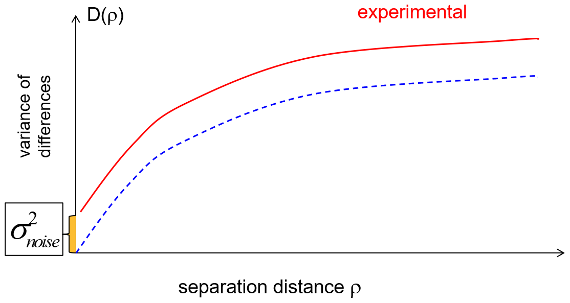
Figure 1 The schematic representation of the structure function estimated from noisy measurements.

This constitutes the principle of the proposed method: at very small separations, the estimation of the structure function will tend towards random error variance. This can be considered as an experimental random uncertainty estimate, ex post in the terminology of von Clarmann et al. (2020). The application of the structure function method requires many measurement points with different spatial and temporal separations, including very small separations, and these measurements should have nearly the same random uncertainties. For satellite measurements in limb-viewing geometry, such information is very limited. Nevertheless, several applications using this method have been published. Staten and Reichler (2009) applied this method to the validation of radio-occultation measurements by the Constellation Observing System for Meteorology, Ionosphere, and Climate (COSMIC), which consists of identical instruments on board of six microsatellites. In their work, the authors evaluated two-dimensional structure function using the data from the beginning of COSMIC mission, when the satellites were in close orbits (and therefore measurements in close separations were found). An analogous method – evaluation of the one-dimensional structure function in polar regions (with transformation of temporal mismatch to spatial separation) – has been applied for validation of random uncertainty estimates of the MIPAS (Michelson Interferometer for Passive Atmospheric Sounding) and GOMOS (Global Ozone Monitoring by Occultation of Stars) instruments on board the Envisat satellite (Laeng et al., 2015; Sofieva et al., 2014). The one-dimensional structure function has been evaluated in Sofieva et al. (2008) using collocated temperature profiles by radiosondes at Sodankylä.

For satellite measurements in nadir-viewing geometry, the smallest separation is usually defined by the ground pixel size of an instrument, and the application of the structure function method looks very attractive: measurements with small spatiotemporal mismatch can be found in all locations and in all seasons. However, we are not aware of the application of the structure function method for validation of random uncertainty estimates from nadir-viewing satellite instruments. In our paper, we use total ozone measurements by TROPOMI on board Sentinel-5P, which has a very fine spatial resolution, for the illustration of the structure function method.

3 Case study: total ozone data by TROPOMI

The TROPOMI satellite instrument on board the Copernicus Sentinel-5 Precursor (S5P) satellite was launched in October 2017 (http://www.tropomi.eu, last access: 15 April 2021; https://sentinel.esa.int/web/sentinel/missions/sentinel-5p, last access: 15 April 2021; Veefkind et al., 2012). The mission of S5P is to perform atmospheric measurements with high spatiotemporal resolution for monitoring air quality and forecasting climate. TROPOMI implements passive remote sensing techniques by measuring the solar radiation reflected, scattered and radiated by the Earth–atmosphere system at ultraviolet, visible, near-infrared and shortwave infrared wavelengths in the nadir-looking geometry. With a large spectral range covered, TROPOMI data allow vertical columns for a wide number of atmospheric gases to be measured, including ozone (O₃), nitrogen dioxide (NO₂), sulfur dioxide (SO₂), carbon monoxide (CO), methane (CH₄) and formaldehyde (HCHO), with an extremely good spatial resolution (3.5 × 5.5 km² since August 2019). This allows the structure function method to be applied, since the ground pixel separations can be probed at very small scales.

The data are available in near-real-time, offline and reprocessing streams. In our studies, the Level 2 offline data product of the total ozone column (TOC) is used. This product relies on the operational implementation of the GODFITv4 algorithm, used for producing total ozone climate data records from many nadir-viewing sensors (GOME (Global Ozone Monitoring Experiment), SCIAMACHY (SCanning Imaging Spectrometer for Atmospheric CHartographY), GOME-2, OMI (Ozone Monitoring Instrument), OMPS (Ozone Mapping and Profiler Suite)) with excellent performance (Garane et al., 2019; Lerot et al., 2014). Total ozone columns are derived using a non-linear minimization procedure of the differences between measured and modeled sun-normalized radiances in the ozone Huggins bands (fitting window: 325–335 nm).

The total ozone product includes an estimate for the random uncertainty associated with each observation. The latter is simply obtained by the propagation through the inversion solver of the radiance and irradiance statistical errors provided with the measurements (in Level 1 products). In addition to the instrumental noise, some pseudo-random errors (i.e., systematic errors varying rapidly at short spatiotemporal scales, “model errors” in the terminology of von Clarmann et al., 2020) may be present in the data due to imperfect corrections for the presence of clouds in the probed scene. In order to limit this term, our main analysis will focus on the clear-sky conditions. We use the operational TROPOMI cloud product (Loyola et al., 2018) to select ozone data with cloud fraction smaller than 0.2.

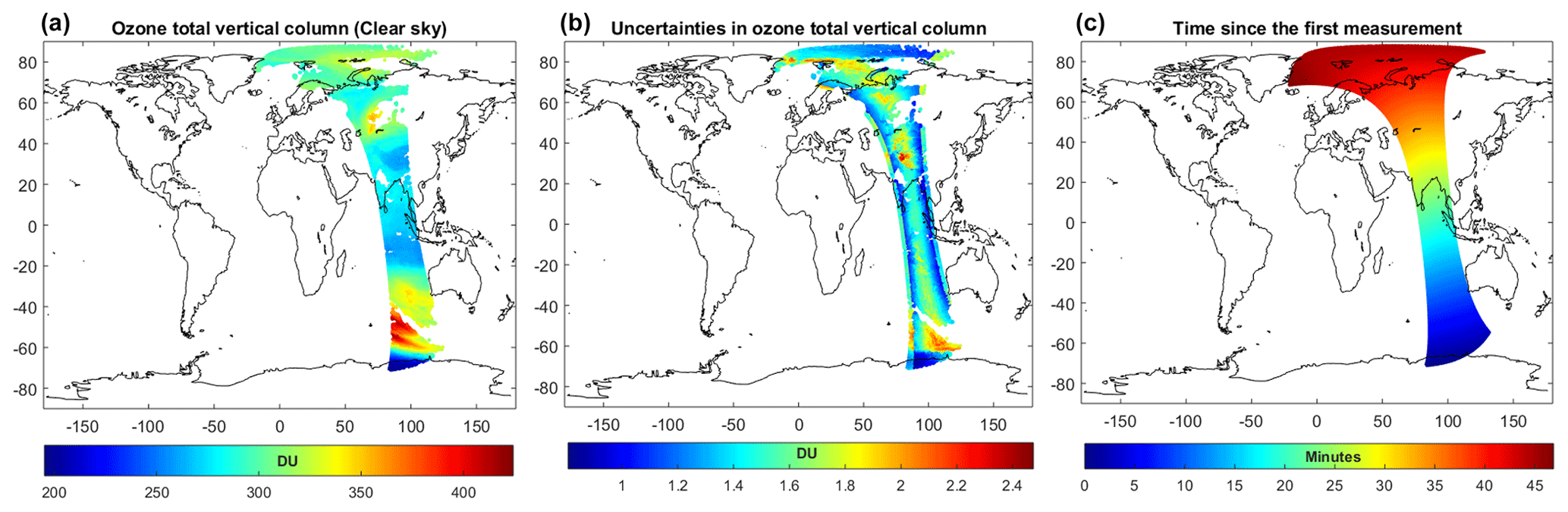
Figure 2 (a) TROPOMI clear-sky ozone measurements in one orbit (1 September 2018, 06:37 UTC). (b) Uncertainties. (c) Time since the first measurement in this orbit.

Figure 2 shows typical TROPOMI clear-sky total ozone column observations in one orbit. Typical values of random uncertainties (Fig. 2, center) range from 0.5 to 2 DU. As shown in Fig. 2 (right), the measurement points in a certain latitude band are performed nearly at the same time, for one orbit.

4 Evaluation of ozone structure functions using TROPOMI data

In our analyses, we selected the TROPOMI Level 2 clear-sky total ozone data in several broad latitude bands (60–90^∘ S, 30–60^∘ S, 20^∘ S–20^∘ N, 30–60^∘ N, 60–90^∘ N) and in certain months: July 2018, October 2018, January 2019 and March 2019. Since the ozone natural variability is expected to depend on latitude and season, we computed the structure function for each latitude band and for each month separately. The sun-synchronous satellite measurements do not allow probing of all temporal separations (the measurements are performed in close local time); therefore in our analysis only spatial separations are studied. In order to exclude the temporal dependence, we evaluated the structure functions for each orbit separately and then averaged over a month. In our work, we evaluate two-dimensional structure function, i.e., the variance of ozone differences as a separation in latitude and in longitude.

The computation of structure function requires finding the differences in ozone and the corresponding spatial separation (i.e., distance in latitude and longitude) between every pair of data pixels. Theoretically it could be achieved by considering one point and comparing it with the rest of observations, then moving to another point and again comparing it with all other observations. However, owing to the very high spatial resolution of TROPOMI and thus an extremely large amount of observation points even for one orbit, such an operation is very demanding computationally. To ensure numerical efficiency, the algorithm is simplified while preserving the underlying principle: instead of using all observations we consider a sufficiently large amount of observations. For each orbit and for each latitude band, we create a set of ∼ 100 reference points evenly spatially spaced in a selected latitude zone. For each reference point, we computed differences from all points in the latitude zone in both longitudinal and latitudinal directions. This operation allows many pairs of data corresponding to all separation distances to be collected (2–2.5 million).

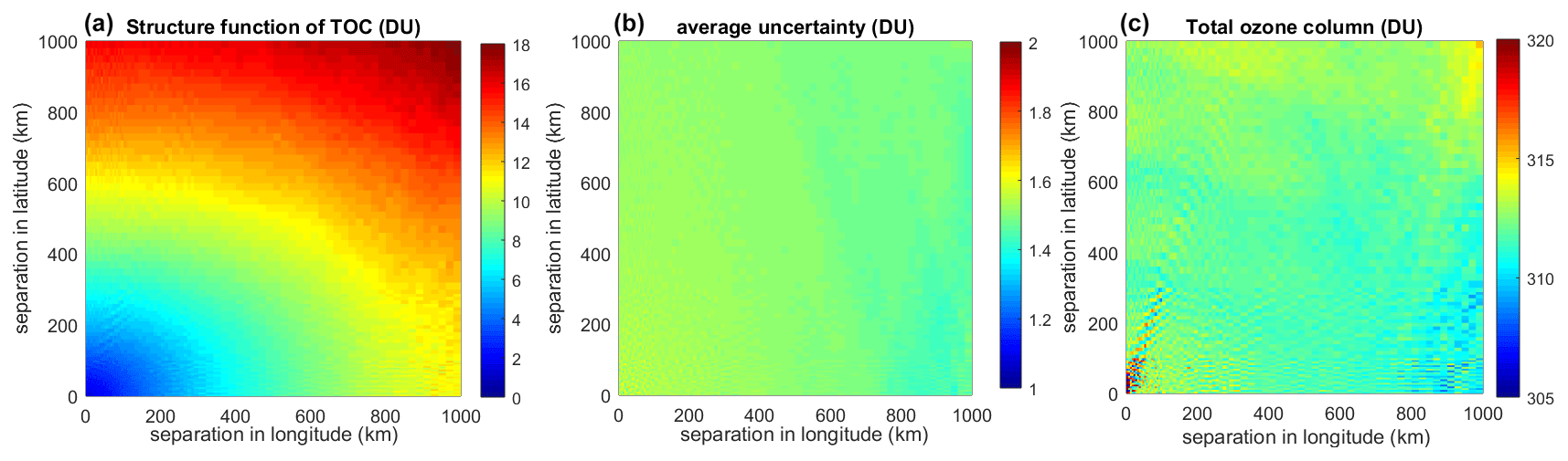
Figure 3 Illustration of structure function in July 2018 and other associated parameters, for latitude 30–60^∘ N. (a) The structure function expressed as $\sqrt{D\left(\mathit{\rho }\right)}$ (DU). (b) Mean uncertainty (DU) corresponding to the separations (pairs of points). (c) Mean ozone column (DU) corresponding to the separations.

After computing the average of the squared difference in ozone and spatial separation for each orbit, the monthly-averaged structure functions are created. The monthly average is based on 400–450 structure functions from individual orbits, so in total 800–1000 million data pairs are used for evaluation of monthly averaged structure functions. The smallest bin for evaluation of the structure function is 5 km × 5 km, and the corresponding sub-sample contains over 14 000 pairs.

Figure 3a shows the example of the structure function evaluated for July 2018 in the latitude band 30–60^∘ N. As expected, the root mean square (rms) of the ozone differences grows with increasing separation distance. The structure function is anisotropic: it is larger in the latitudinal direction. In the selected latitude band (this is also the case for other months and latitude bands), the mean error estimate corresponding to different separation distances is nearly constant (∼ 1.5 DU, Fig. 3b). Analogously, the mean ozone value in the pairs corresponding to different separation distances is also nearly constant (Fig. 3c), as expected. This implies that the structure function looks similar in both absolute (DU) and relative (%) representations (see also below).

5 Results and discussion

The structure functions evaluated in different latitude bands and seasons are shown in Fig. 4. Color represents $\sqrt{D\left(\mathit{\rho }\right)}$ expressed in DU. An analogous figure showing the structure function in relative units (%) is presented in Fig. A1 in the Appendix. As mentioned above, the structure functions in absolute and in relative units look very similar.

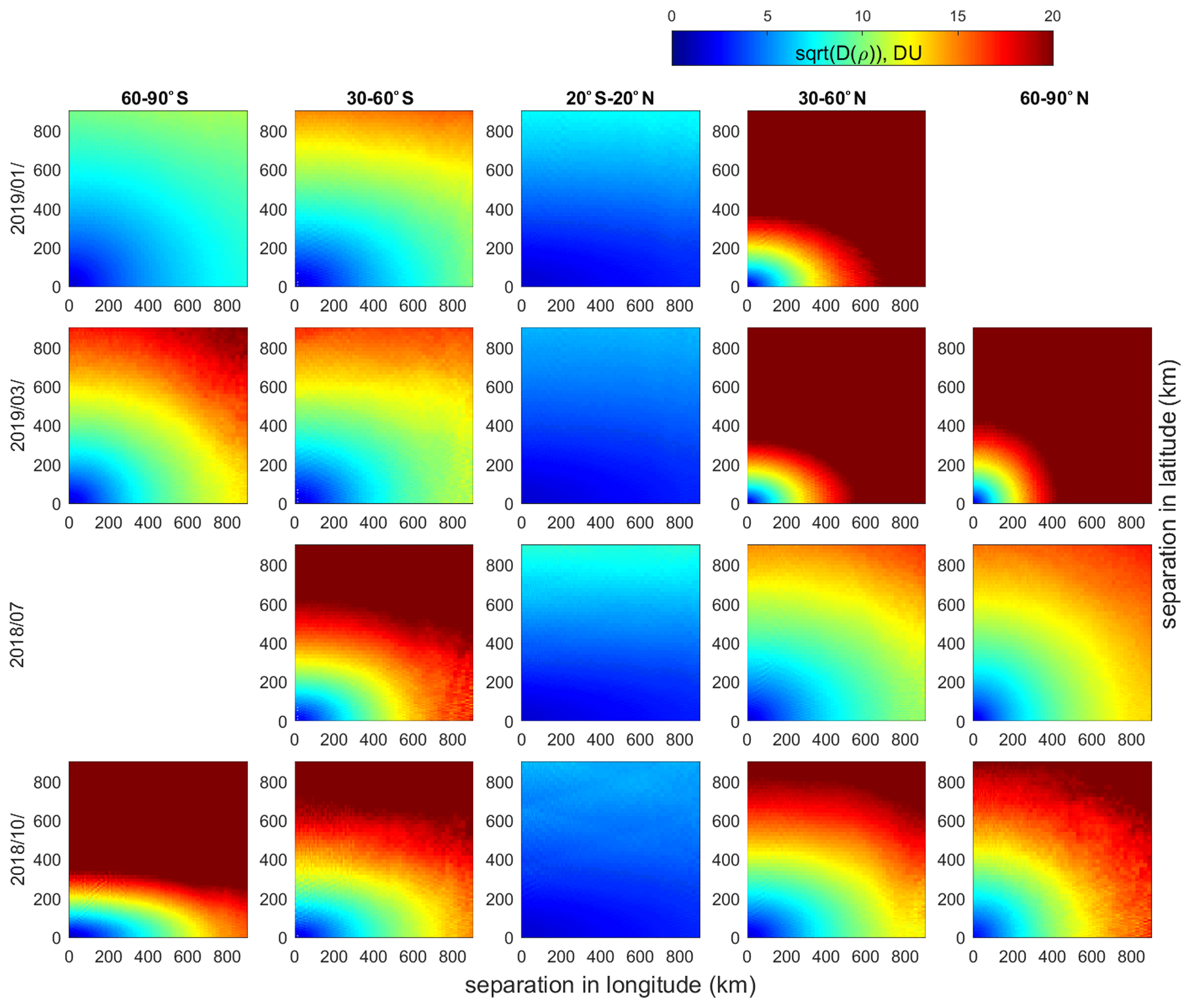
Figure 4 Structure function (expressed as $\sqrt{D\left(\mathit{\rho }\right)}$ in DU) for different latitude bands (columns) and months (rows).

The obtained morphology of ozone variability is quite expected: it is overall much smaller in the tropics than at middle and high latitudes, where it has a pronounced seasonal cycle. At mid-latitudes in winter and spring, the ozone variability is very strong, even for small separations. Except at high northern latitudes in winter and spring, the structure functions are anisotropic with a stronger variability in the latitudinal direction.

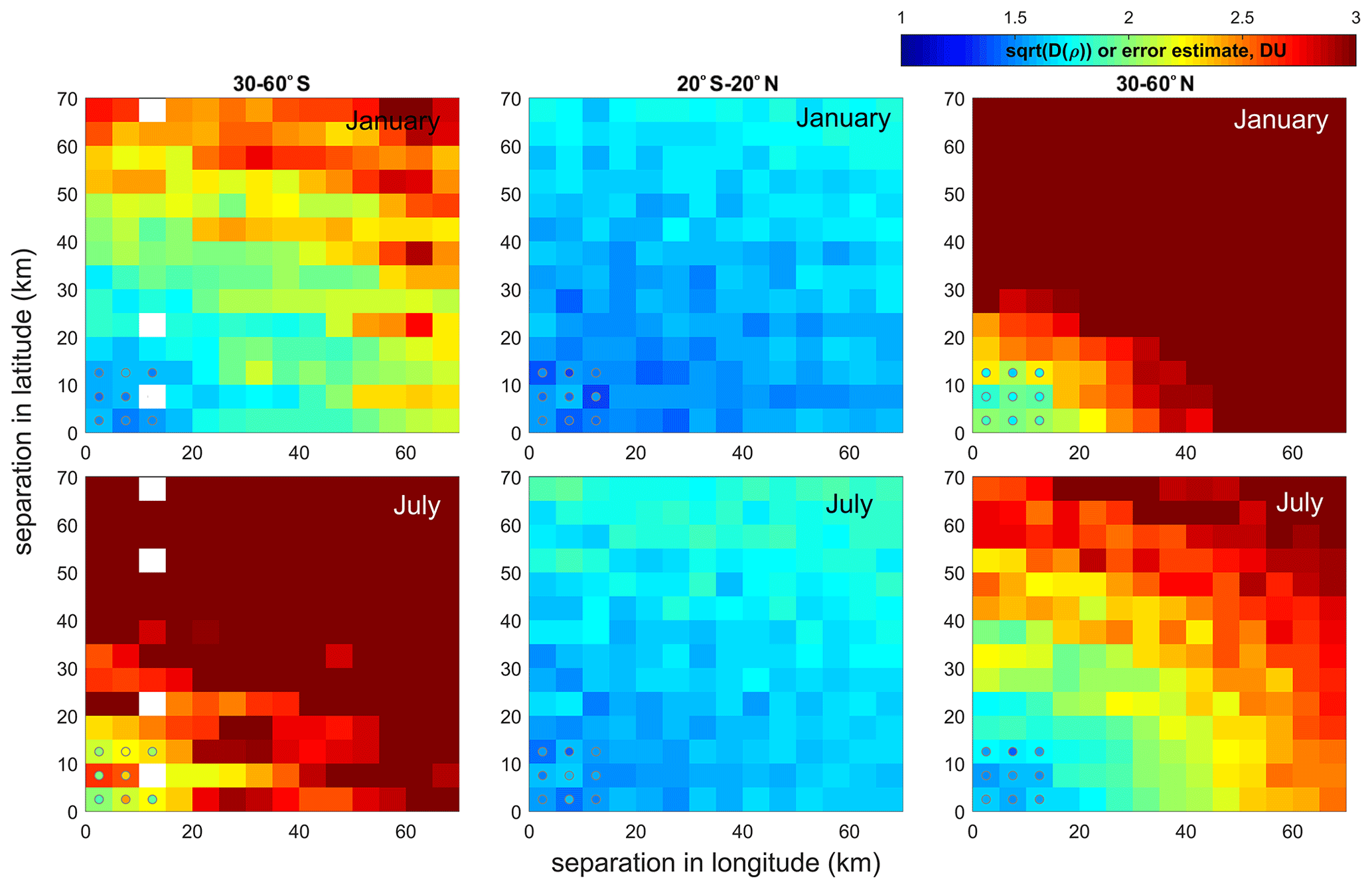
Figure 5 Structure function (in DU) for different latitude bands (columns) and months (rows), with the focus on small separations. Colored circles at the origin indicate the uncertainty estimates (ex ante) given by the inversion algorithm.

Figure 5 shows the structure functions for selected latitude zones (the same as presented in Fig. 4), but with the focus on small separations, for January 2019 and July 2018. In Fig. 5, the colored circles near the origin indicate the mean (for the corresponding latitude zone and month) ex ante uncertainty estimates in the pairs with small separation distances. We observe that in the regions of small (20^∘ S–20^∘ N) or moderate variability (30–60^∘ S and 30–60^∘ N in local summer), the structure function values at the zero limit are nearly identical to the theoretical random error estimates in the data. This indicates that the random uncertainty estimates provided by the inversion algorithm are close to reality. In the regions of large ozone variation (mid-latitudes in local winter), the structure function grows so rapidly that it has the values comparable with theoretical ex ante uncertainties only for very small separation distances.

The distribution and statistical parameters of experimental uncertainty estimates using the structure function method (ex post) and the theoretical uncertainty estimates provided by the inversion algorithm (ex ante) in the tropics and at mid-latitudes are shown in Fig. 6. The individual values of the structure function and ex ante uncertainties (black dots in Fig. 6) are selected for small separations: 20 × 20 km latitude-longitude separation distance in tropics (all seasons), 15 km × 15 km in summer–autumn at mid-latitudes and 5 km × 5 km in winter–spring at mid-latitudes. The statistical parameters of the distributions – the mean and median values in percentiles – are also shown in Fig. 6. In the tropics, ex post and ex ante uncertainty estimates are in very good agreement; they are ∼ 1.5 DU. At mid-latitudes, the distribution of ex post uncertainty estimates is slightly shifted toward larger values compared to the distribution of ex ante uncertainties, but the difference in the mean values is small, less than ∼ 0.1 DU, and the 16th–84th inter-percentile ranges overlap.

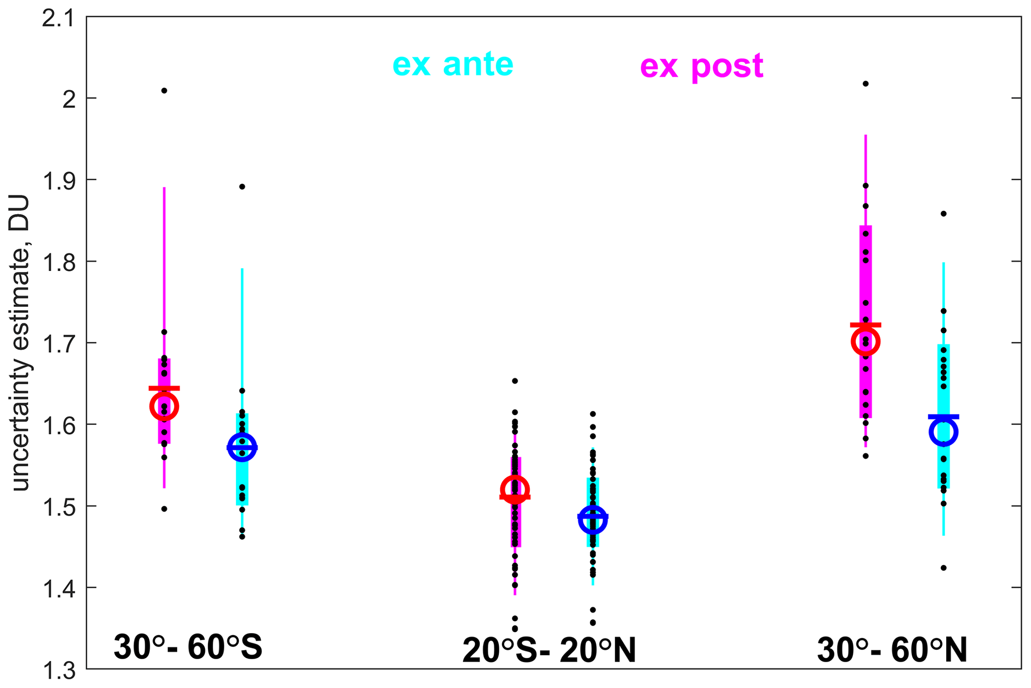
Figure 6 The distributions of experimental uncertainty estimates using the structure function method (ex post: magenta and red color) and the theoretical values by the inversion algorithm (ex ante: cyan and blue color) in the tropics and at mid-latitudes. Black dots show individual values, circle is median, horizonal dash is mean, thick vertical lines span over 16th–84th inter-percentile range, thin vertical lines span over 5th–95th inter-percentile range of the uncertainty estimates.

The structure function method is also a powerful tool for detecting non-accounted pseudo-random errors. To demonstrate this, we compare in Fig. 7 the structure functions in the tropics for TROPOMI ozone data in clear-sky and cloudy conditions (cloud fraction > 0.2). In cloudy conditions, the pseudo-random errors due to the presence of clouds are not characterized by the inversion algorithm at the moment; therefore it is expected that the structure function is higher at zero separations than ex ante uncertainty estimates. This is clearly observed in Fig. 7: in cloud-free conditions, the nugget of the structure function nearly coincides with the ex ante uncertainty estimates, while in cloudy conditions it is substantially higher, thus indicating the presence of additional pseudo-random uncertainties.

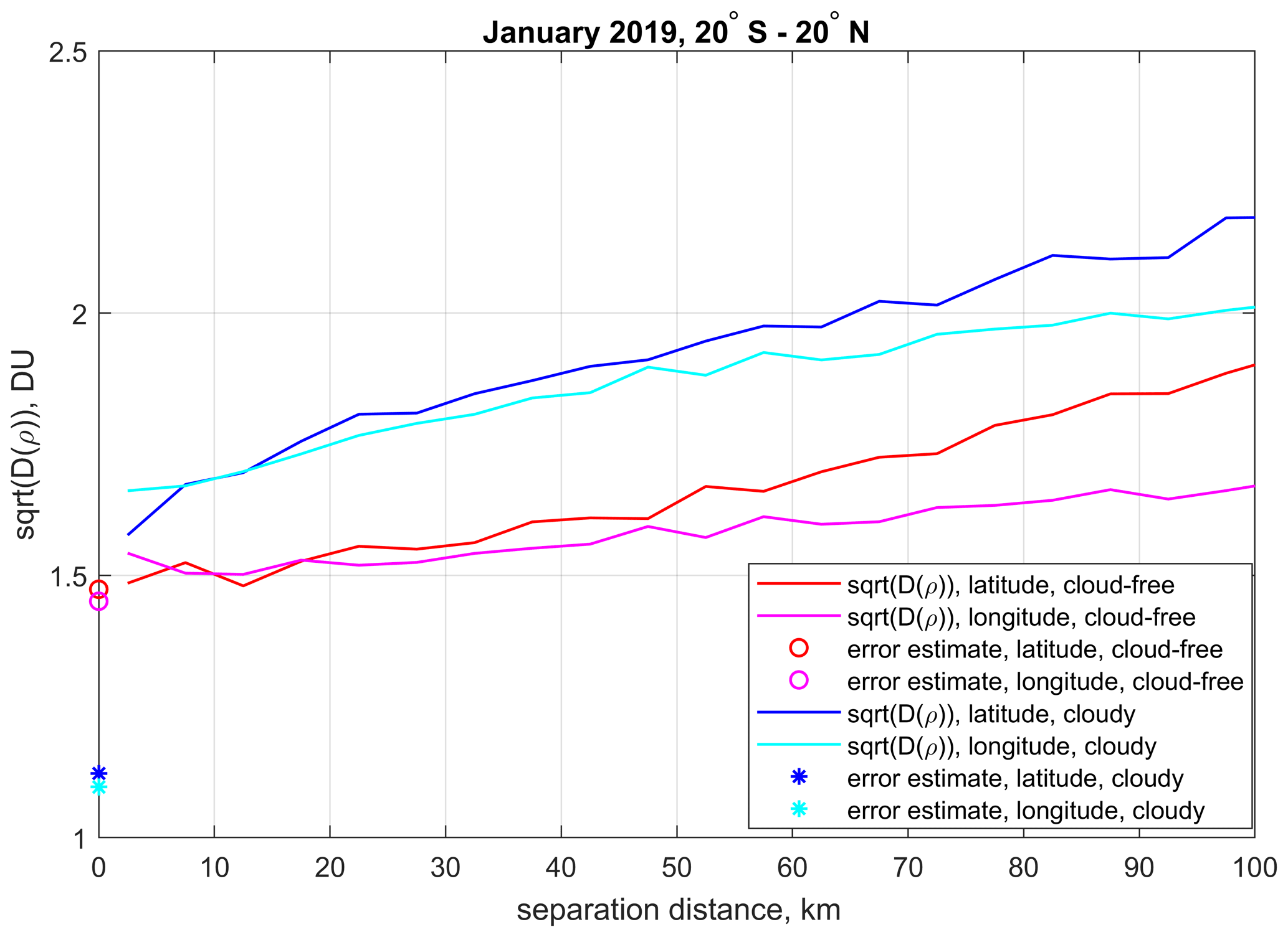
Figure 7 One-dimensional structure functions in latitude and in longitude separations (color lines), which are computed from a two-dimensional structure function like in Fig. 4 by averaging over longitude–latitude separations from 0 to 20 km. The symbols at zero separations indicate ex ante uncertainty estimates.

It is quite evident that the structure function method can be applied to any dataset in which data with different separation distances can be found. The approach might especially be useful for other remote sensing measurements in nadir-looking geometry, which have fine horizontal resolution. The datasets should not be necessarily remote sensing measurements. The structure function can also be applied, for example, to modeled data by a chemistry-transport model, in order to estimate numerical noise in the model.

6 Summary

The analyses performed in our paper have shown that the structure function method – i.e., the evaluation of rms differences as a function of increasing spatial separation – is a powerful tool, which allows quantification of random noise in the data. The limit at zero mismatch provides the experimental estimate of the random uncertainty variance. In our paper, we applied the structure function method to validate the TROPOMI clear-sky total ozone random uncertainty estimates by the inversion algorithm. We found that the latter are very close to the experimental ones provided by the structure function method, in the regions of small total ozone natural variability. This indicates adequacy of the TROPOMI random error estimation.

At the same time, the structure function method provides the detailed information about the natural variability of the measured parameter. For TROPOMI total ozone, we have analyzed the structure functions in different seasons and latitude zones. We found the expected results: the overall variability is the smallest in the equatorial region, and the largest variability is at middle and high latitudes in winter and spring. At these locations and during these seasons, the rms of ozone differences grows rapidly with the separation between measurements achieving ∼ 5 % at distances of 300–500 km. Our analysis has shown that the structure function is anisotropic (variability is larger in the latitudinal direction) at separations of a few hundred kilometers nearly everywhere, except at northern polar regions. For lower separation distances (up to 20–40 km), the structure function generally remains isotropic.

The structure function method is also a powerful tool for detecting non-accounted pseudo-random errors. In the paper, we have demonstrated this by comparing the structure functions and theoretical uncertainty estimates for TROPOMI ozone measurements in clear-sky and cloudy conditions.

The structure function method discussed in the paper can be equally applied to other remote sensing measurements or atmospheric model data.

Appendix A

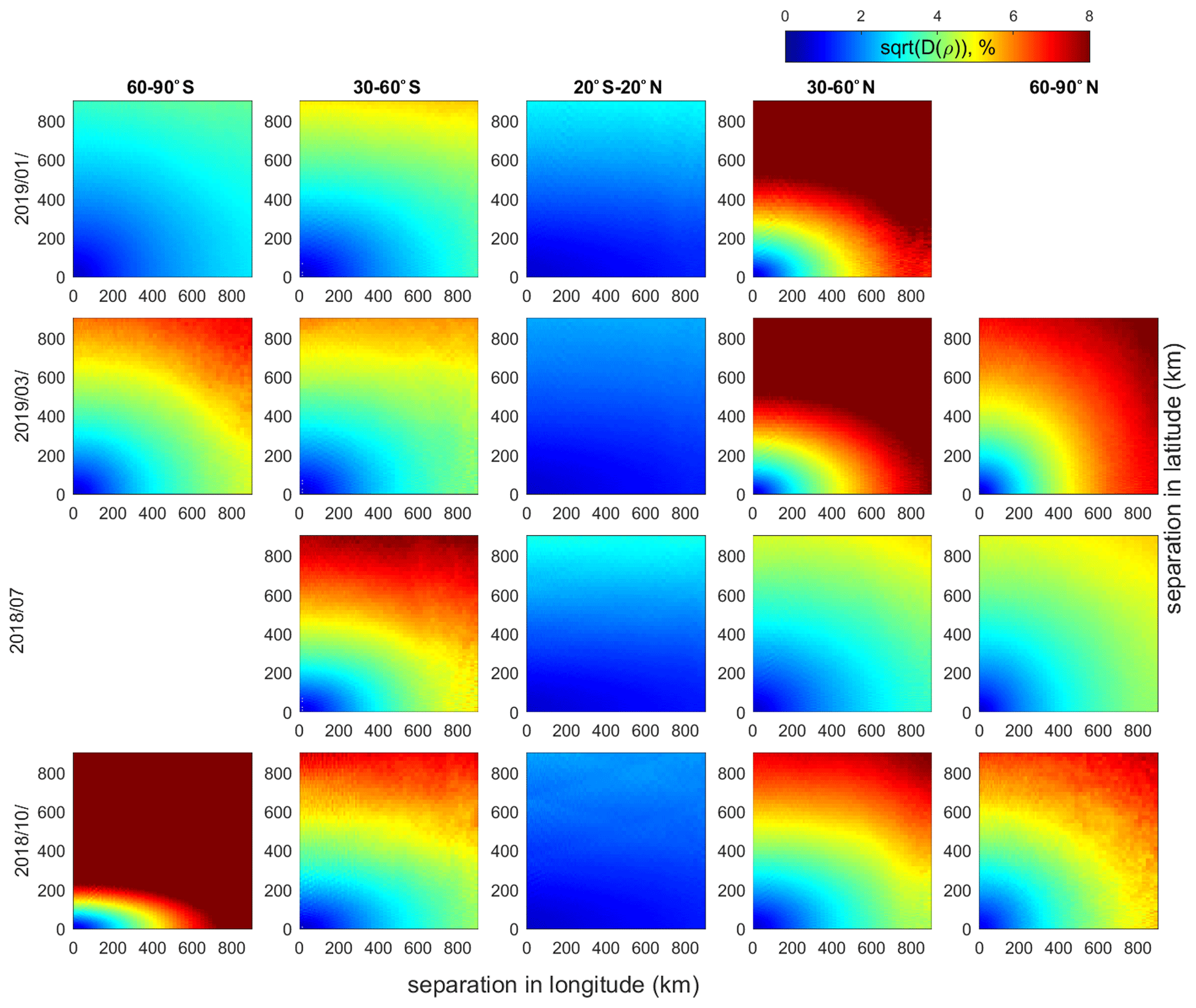
Figure A1 Structure function (in %) for different latitude bands (columns) and months (rows).