the Creative Commons Attribution 4.0 License.
the Creative Commons Attribution 4.0 License.
 | 22 Apr 2021
Statistically analyzing the effect of ionospheric irregularity on GNSS radio occultation atmospheric measurement
Mingzhe Li
Xinan Yue
The Global Navigation Satellite System (GNSS) atmospheric radio occultation (RO) has been an effective method for exploring Earth's atmosphere. RO signals propagate through the ionosphere before reaching the neutral atmosphere. The GNSS signal is affected by the ionospheric irregularity including the sporadic E (Es) and F region irregularity mainly due to the multipath effect. The effect of ionospheric irregularity on atmospheric RO data has been demonstrated by several studies in terms of analyzing singe cases. However, its statistical effect has not been investigated comprehensively. In this study, based on the Constellation Observing System for Meteorology, Ionosphere, and Climate (COSMIC) RO data during 2011–2013, the failed inverted RO events occurrence rate and the bending angle oscillation, which is defined as the standard deviation of the bias between the observed bending angle and the National Center for Atmospheric Research (NCAR) climatology model bending angle between 60 and 80 km, were used for statistical analysis. It is found that at middle and low latitudes during the daytime, the failed inverted RO occurrence and the bending angle oscillation show obvious latitude, longitude, and local time variations, which correspond well with the Es occurrence features. The F region irregularity (FI) contributes to the obvious increase of the failed inverted RO occurrence rate and the bending angle oscillation value during the nighttime over the geomagnetic equatorial regions. For high latitude regions, the Es can increase the failed inverted RO occurrence rate and the bending angle oscillation value during the nighttime. There also exists the seasonal dependency of the failed inverted RO event and the bending angle oscillation. Overall, the ionospheric irregularity effects on GNSS atmospheric RO measurement statistically exist in terms of failed RO event inversion and bending angle oscillation. Awareness of these effects could benefit both the data retrieval and applications of RO in the lower atmosphere.
- Article
(2726 KB) - Full-text XML
- BibTeX
- EndNote


Radio occultation (RO) is a technique originally developed in the late 1960s and early 1970s for planetary atmosphere exploration. With the great development of the Global Navigation Satellite System (GNSS) over the past 30 years, the GNSS signal has been an effective source for exploring the Earth's atmosphere. Several RO missions such as the Global Positioning System Meteorology (GPS/MET), the Challenging Minisatellite Payload (CHAMP) (Wickert et al., 2001), the Scientific Application Satellite-C (SAC-C), the Gravity Recovery and Climate Experiment (GRACE) (Beyerle et al., 2005), the Constellation Observing System for Meteorology, Ionosphere and Climate (COSMIC) (Schreiner et al., 2007), the Meteorological Operational Satellite Program (Metop) A/B, and the Fengyun-3C (FY-3C) (Mao et al., 2016) have proven the good capability of RO for observing the Earth's ionosphere and atmosphere. High-quality products of RO have been used for space weather, weather, and climate research (Anthes et al., 2008).
The RO technique can be divided into the ionospheric RO and the atmospheric RO. For the former, the GNSS signal propagates through the ionosphere. Dual-frequency pseudorange and carrier phase can be observed by the receiver onboard the low Earth orbit (LEO) satellite and used to invert the electron density profile. In addition, the amplitude and phase measurements can be used to calculate the ionospheric scintillation index such as the S4 index. The S4 index is defined as the standard deviation of the received signal power normalized to the average signal power; it can represent the occurrence of the ionospheric irregularity (Yue et al., 2016). For the latter, the GNSS signal propagates through both the ionosphere and the neutral atmosphere. The dual-frequency carrier phase can be used to calculate the bending angle and then invert the atmospheric parameters. As a result, the effect on signals caused by the ionosphere should be removed before deriving the atmospheric RO products.
For atmospheric RO, the GNSS signal is mainly affected by the ionosphere in two ways. Firstly, the existence of dense ionospheric electron density contributes to the bending of signals. Similar to the first-order ionospheric term calibration used in ground-based dual-frequency observations, a linear combination of the two-band signal bending at the same impact parameter is usually used to remove the ionospheric effect (Vorob'ev and Krasil'nikova, 1994). However, after the linear combination of bending angles, there still exists a residual ionospheric error (RIE). The RIE could bring ionospheric variability such as solar cycle, local time, and seasonal variations into atmospheric RO products although its amplitude is relatively low (Li et al., 2020). It means that the climate research using atmospheric RO products would be affected by the ionosphere. Some efforts have been made for RIE calibration (Danzer et al., 2013, 2015, 2020; Healy and Culverwell, 2015; Angling et al., 2018; Liu et al., 2018, 2020; Li et al., 2020). Danzer et al. (2013) have analyzed the bending angle bias of CHAMP and COSMIC RO data from 2001–2011 and tried to parameterize bending angle bias versus the solar cycle to make statistical corrections. Healy and Culverwell (2015) found a good correlation between the RIE and the difference between GPS L1 and L2 bending angles at the same impact parameter. They then proposed a correction method using the “kappa” parameter under the ionospheric spherical symmetry assumption. This method was further tested by Danzer et al. (2015), Angling et al. (2018), and Danzer et al. (2020). It can reduce the systematic error variation with the solar cycle from 0.2 to 2.0 K at altitudes between 40 to 45 km. Liu et al. (2018) have analyzed the ionospheric structure influences on RIE in bending angles based on ray tracing simulations and further developed a “bi-local correction approach” to calculate the RIE through an equation. This method considers both the ionospheric asymmetry effects as well as the geomagnetic effects on bending angles (Liu et al., 2020). In our previous study, we have also characterized the RIE effects statistically by both ray-tracing simulation and data analysis (Li et al., 2020). Secondly, the small-scale irregularities in the ionosphere also have an impact on the GNSS signal and finally affect the atmospheric RO products. The small-scale irregularities of interest to this study are the sporadic E (Es) and F region irregularity (FI). As indicated by former studies, the ionospheric irregularity will cause refraction or diffraction of the GNSS signal during its propagating through the ionosphere. The received signals could show temporal fluctuations in both amplitude and phase, which is known as the ionospheric scintillation. The impact of the small-scale irregularity on atmospheric RO can be significant but show quite different climatological characteristics in comparison with the large-scale ionospheric effects (Li et al., 2020). In addition, it is difficult to model the ionospheric irregularity in a deterministic fashion for simulation research (Mannucci, et al., 2011). Previous studies only pointed out this small scale ionospheric effect in terms of cases (Zeng and Sokolovskiy, 2010). To our knowledge, there is no comprehensive study giving statistical analysis of ionospheric irregularity and atmospheric RO products, which is quite important to quantify this effect and therefore benefit atmospheric RO data retrieval and application. This is the main objective of this study.
In the following sections, we mainly study the ionospheric irregularity effects on GNSS atmospheric RO measurement statistically. Based on previous related studies, the current study is useful regarding the following aspects: (1) the correlation between failed inverted COSMIC RO events and the ionospheric irregularity are analyzed, (2) morphology of the bending angle oscillation in the atmospheric RO measurement are presented in comparison with the occurrence rate of both Es and FI, and (3) the seasonal dependency of failed inverted RO events and the bending angle oscillation are analyzed. We will describe the COSMIC observation and the statistical method in Sects. 2 and 3, respectively. Then the ionospheric irregularity effects on single RO cases will be shown in Sect. 4. The statistical results of the failed inverted RO event and the bending angle oscillation will be depicted in comparison with the ionospheric irregularity occurrence rate in Sect. 5. Finally, the conclusions and implications will be presented in Sect. 6.
COSMIC, one of the most successful RO missions, was launched on 15 April 2006. The constellation with six LEO satellites has contributed millions of profiles for space weather, weather, and climate research in the past 14 years. Each COSMIC satellite has four separate antennas: two high-gain occultation antennas receive GNSS signals with a 50 Hz sampling rate to explore the neutral atmosphere from the top (∼130 km) to the bottom or vice versa. The carrier phase modulated on signals can be used for excess phase calculating and atmospheric parameter retrieving. The other two antennas are precise orbit determination (POD) antennas with a 1 Hz sampling rate. The received signals are used for LEO orbiting, ionosphere electron density, slant total electron content (TEC), and scintillation index calculating (Schreiner et al., 2007, 2011). The COSMIC data are processed by the COSMIC Data Analysis and Archive Center (CDAAC) of the University Corporation for Atmospheric Research (UCAR) and available on the CDAAC website (https://www.cosmic.ucar.edu/what-we-do/cosmic-1/data, last access: 17 April 2021). In this study, the COSMIC RO observations during 2011–2013 were used for analysis. The S4 scintillation index in auxiliary data file (scnLv1) was used for the Es and FI occurrence rates calculation. The dry atmospheric profiles file (atmPrf) was used for the failed inverted RO occurrence rate calculation and the atmospheric bending angle oscillation morphology analysis. The specific calculation method will be introduced in the following section.
To study the ionospheric irregularity effects on RO, we focus on analyzing two parameters: the failed inverted RO event occurrence rate and the bending angle oscillation defined as the mean standard deviation of the bias between the observed bending angle and the NCAR climatology model bending angle during the 60–80 km altitude interval. The failed inverted RO event means those events flunked the quality control during profiles inversion in CDAAC. They are identified by the “bad” attribute in the atmPrf file whose values are equal to 1. The oscillation of atmospheric RO bending angle is also provided by the atmPrf file. The S4 index contained in the scnLv1 file is used to represent the occurrence of the ionospheric irregularity. The occurrence rate of the S4 index larger than 0.3 is set to represent the occurrence of ionospheric irregularity. It should be noted that we identify the occurrence altitude range between 50–600 km as the contribution of both Es and FI together. We first calculated the failed inverted RO event occurrence rate in comparison with the ionospheric irregularity occurrence rate. After that, failed inverted RO events of COSMIC during 2011–2013 were screened out to study the Es and FI effects on the bending angle observation. Additionally, the ionPrf file of CDAAC is used for displaying the electron density profiles in single cases.
To obtain preliminary knowledge of the ionospheric irregularity effect on atmospheric RO, we firstly show several typical single case examples. The results are shown in Fig. 1. From top to bottom, each row shows the results of a case. The three cases represent the RO event without ionospheric irregularity, the RO event affected by the Es, and the event affected by the FI, respectively. From left to right, the panels represent the inverted bending angles, the signal-to-noise ratio (SNR) of the L1 coarse-acquisition (C/) signal, the related electron density profile, and the inverted dry temperature profile compared with the European Centre for Medium-Range Weather Forecasts (ECMWF) results. Please note that the gray lines in the rightmost panels denote the results of RO inverted temperature and the red lines represent those of ECMWF. The purple lines in case 1 and case 3 are the temperature bias multiplied by 10 for convenient comparison. The features of the L1 C/A SNR profile and the electron density profile could identify whether an RO event is affected by the ionospheric irregularity (Yue et al., 2015). As depicted in the second column, case 2 shows visible peaks in SNR fluctuation around 110 km, which correspond to the occurrence altitude range of Es and could reflect the Es effects on this event. In addition, the electron density profile of case 3 shows obvious scintillation between 200 and 300 km, which implies the FI impact on signals. We also use the corresponding CDAAC scnLv1 file for verification. The S4 maximum values of cases 1–3 are 0.03, 0.59, and 1.21, with S4 peaks around 111.69, 108.45, and 274.86 km, respectively. It can be seen that the normal case shows good inversion results. The value of the ionospheric-corrected linear-combined (LC) bending angle above 40 km is much smaller than those of the L1 and L2 bending angles. It means that the ionosphere dominates the bending of the RO signal in this tangent altitude interval and the linear combination method works well. The bias between the observed dry temperature and the ECMWF result is insignificant. However, the Es case shows bad results. Values of the inverted L2 bending angle are negative, which leads to larger values of the LC bending angle after the linear combination. As a result, the temperature profile is failed inverted. Significant temperature bias between the observation and model result can be seen from the rightmost panel. For the FI case, oscillations can be seen in the LC bending angle profile in the leftmost panel as well as the temperature bias profile in the rightmost panel. The bending angle oscillation values of cases 1–3 are 0.66, 16.06, and 5.74 murad, respectively. This indicates that this oscillation could also be related to the ionospheric irregularity. The geometry of atmospheric RO observation determines that the ionospheric irregularity effects could propagate to a deep tangent height far below the altitude range of irregularity occurrence (Wu, 2020). We have gone through many cases and found that the failed inverted RO event and strong bending angle oscillation usually occurs along with Es and FI. But not all events affected by the Es and FI are failed inverted. The analysis of single cases motivates our further statistical study.
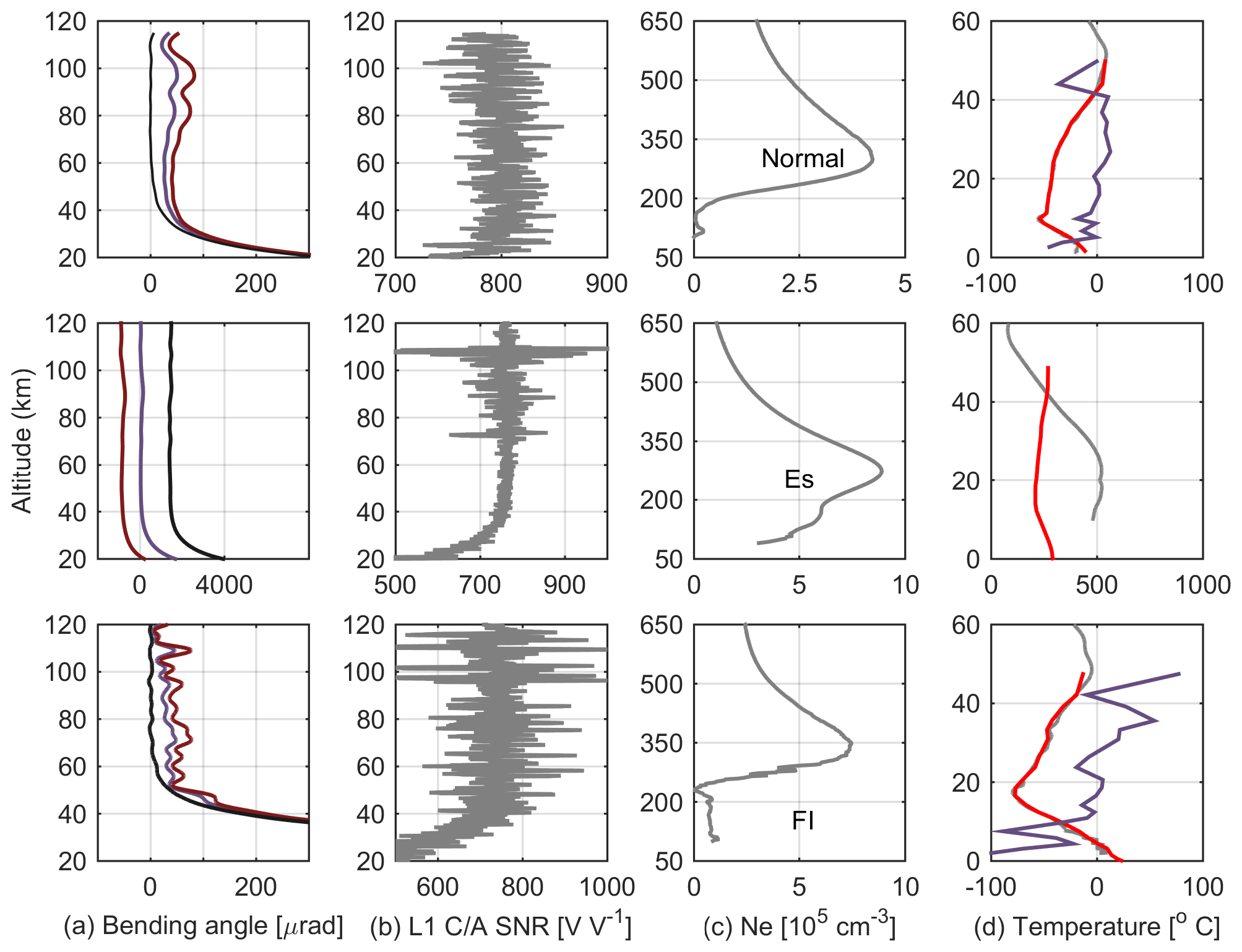
Figure 1Example of three cases in 2013 made by COSMIC. The panels from top to bottom are normal examples without the ionospheric irregularity occurrence, the Es example, and the F region irregularity example. Panels from left to right are (a) the inverted bending angles, (b) the L1 C/A SNR, (c) the electron density profile at the RO tangent points, and (d) the inverted dry temperature (gray line) versus the ECMWF results (red line). The inverted L1 (purple line), L2 (brown line), and LC (black line) bending angles are all depicted in column (a). The purple lines in column (d) represent the bias between the inverted dry temperature and the ECMWF results multiplied by 10. Please note that the y axis of all panels represents the altitude with kilometer (km) as the unit.
The Es and FI have been investigated comprehensively over the past several decades (Hocke et al., 2001; Straus et al., 2003; Wu, 2005; Arras et al., 2008, 2009; Carter et al., 2013; Yue et al., 2015, 2016). Generally, the Es can be seen as thin layers with much higher plasma density than the normal E region density occurring in the altitude range of ∼90–120 km. The occurrence rate of Es is controlled by many factors such as the tidal wind, the Earth's geomagnetic field, and metal ions (Axford, 1963; Chu et al., 2014). These factors lead to the complicated variations of Es along with latitude, longitude, altitude, local time, and season (Hocke et al., 2001; Wu, 2005; Arras et al., 2008, 2009). FI is the plasma irregularity and inhomogeneity in the F region caused by plasma instabilities (Dungey, 1956; Fejer and Kelley, 1980). The scale sizes of the density irregularity range from a few centimeters to hundreds of kilometers and the irregularity can appear at all latitudes. Both Es and FI have been observed by ionosonde, incoherent/coherent scatter radars, and ground-based GNSS networks. Since the success of GPS/MET, the GNSS RO has also been proven as an effective technique to detect the occurrence of Es and FI. Hocke et al. (2001) first derived the occurrence of Es from the GPS/MET observation and confirmed its seasonal variation. Wu (2005) studied the latitude, local time, altitude, and seasonal dependency of Es using CHAMP occultation data. Arras et al. (2008) further investigated the occurrence of Es using multiple RO missions including CHAMP, GRACE-A, and COSMIC. Chu et al. (2014) presented the morphology of Es based on COSMIC amplitude and phase fluctuations of L-band signals. For FI, Straus et al. (2003) made a statistical analysis of the GPS C/A code SNR fluctuations on L1 frequency based on observations onboard the PICOSat satellite. They found that the geographic and local time distributions of occultation having large values of the S4 index were consistent with known scintillation climatology. Brahmanandam et al. (2012) presented the three-dimensional global morphology and seasonal variations of the S4 index measured from COSMIC for 2008, a low solar activity year, and found the latitude, altitude, and local time dependency of FI. Carter et al. (2013) further revealed the longitudinal and seasonal variations of equatorial FI using the COSMIC S4 index. In addition, Yue et al. (2015, 2016) also studied the complex Es and the ionospheric irregularity related GPS RO loss of lock by the COSMIC S4 index.
As investigated in the single case section, the failed inverted RO event and bending angle oscillation could be related to the ionospheric irregularity, so we carried out statistical research from all COSMIC atmospheric events during 2011–2013. Firstly, the RO event whose “bad” attribute in the atmPrf file equals 1 was selected as the failed inverted RO for the statistics. Then the failed inverted RO events were screened out for the bending angle oscillation study. The geographical and geomagnetic distributions of Es and FI are plotted separately in Fig. 2. The mixed Es and FI occurrence rate, the failed inverted RO event occurrence rate, and the bending angle oscillation are shown in Fig. 3. The grid resolutions are 10∘ × 3∘ for Lon × Lat and 3∘ × 2 h for MLat × MLT, respectively.
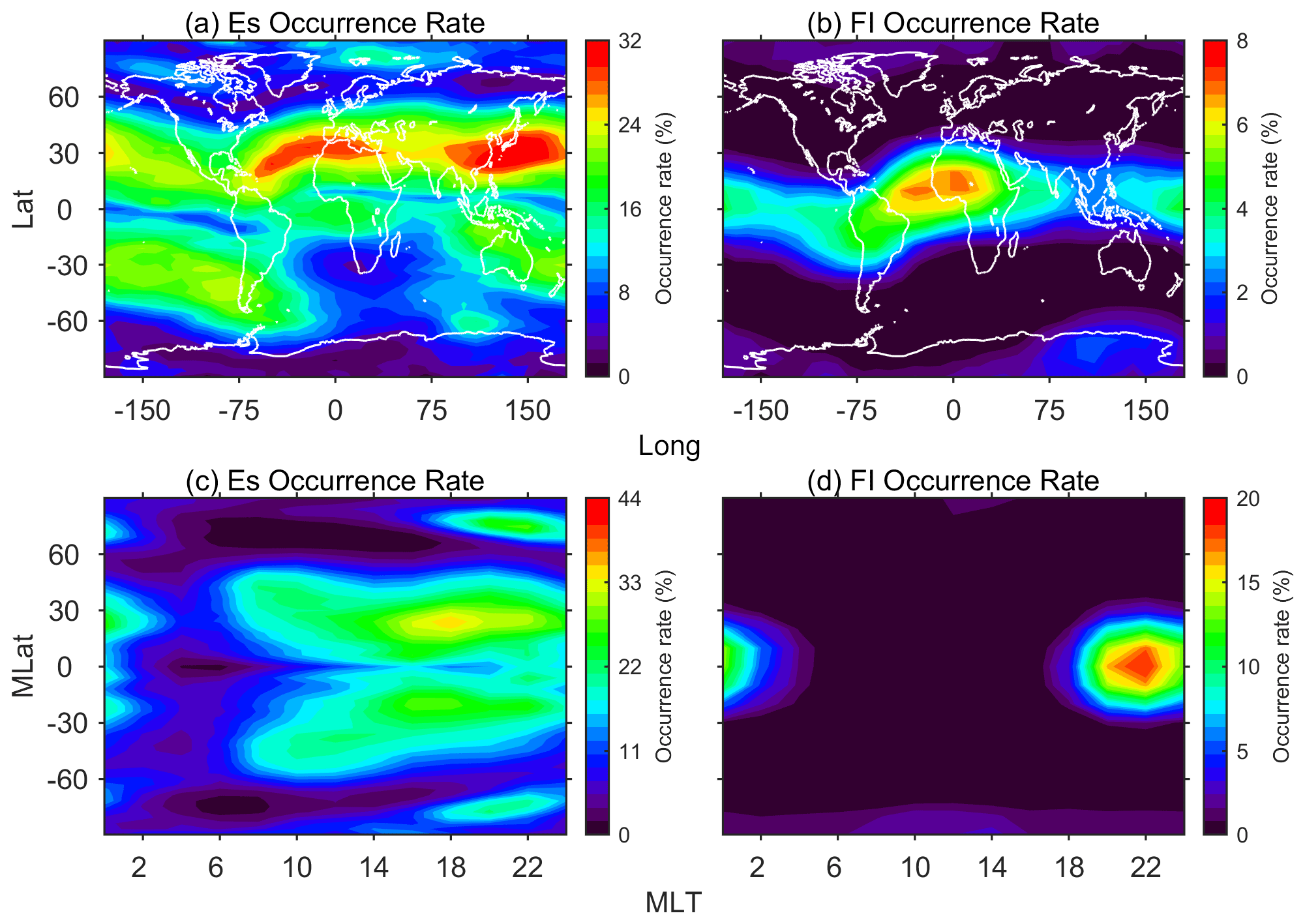
Figure 2Global geographical (a, b) and geomagnetic distributions (c, d) of the Es (a, c) and F layer irregularity occurrence rate (b, d) during 2011–2013.
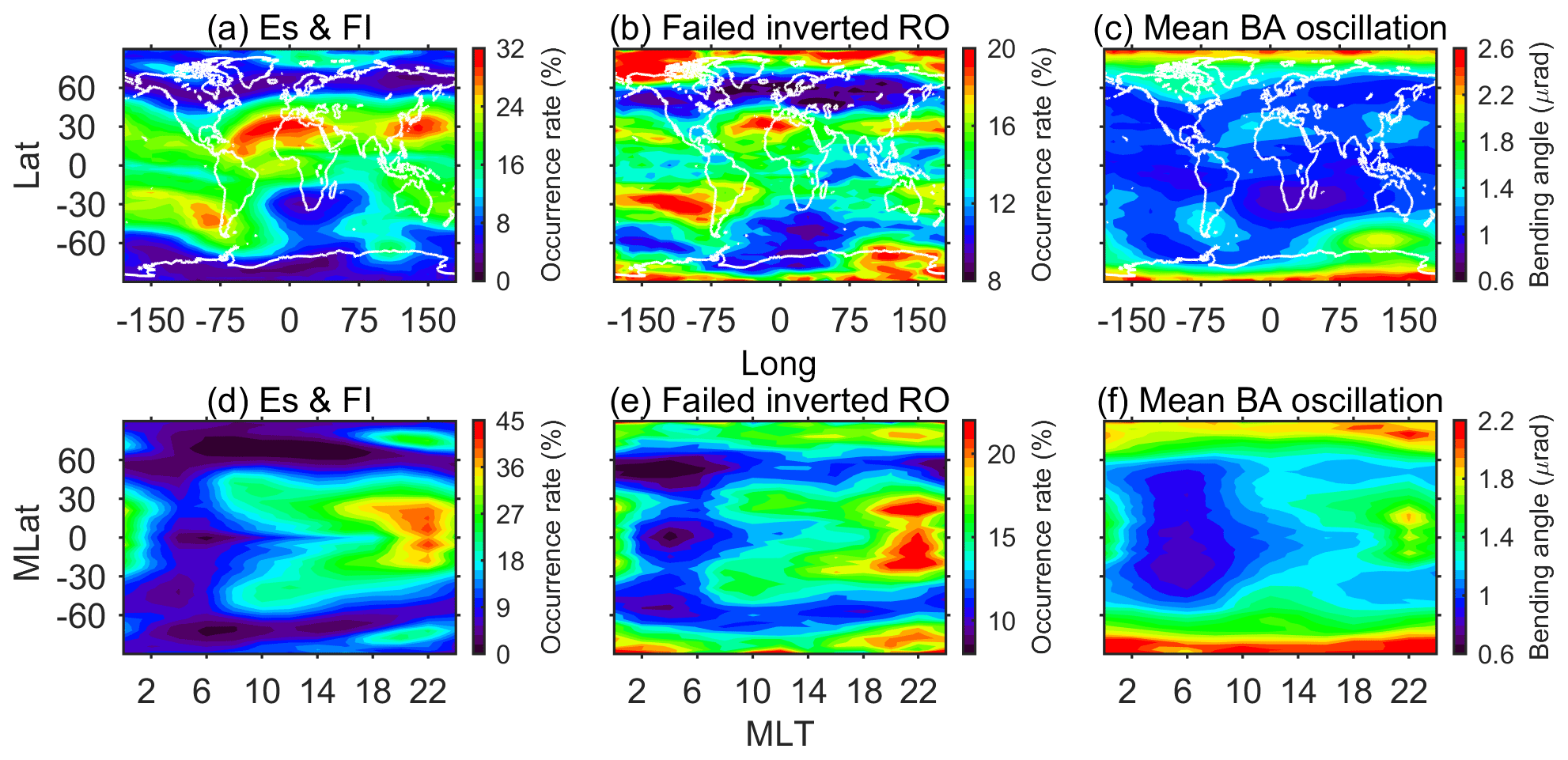
Figure 3Global geographical (a–c) and geomagnetic distributions (d–f) of the Es and F layer irregularity occurrence rate (a, d), the failed inverted RO event occurrence rate (b, e), and the mean bending angle oscillation (c, f) during 2011–2013.
As depicted in Fig. 3, the global geographical distribution of both Es and FI occurrence rate together is depicted in the top left panel. For low and middle latitudes, two peaks of Es occurrence rate are located in the East Asia region and the North Africa region in the northern hemisphere. One peak is located near the South America region. The values of occurrence rate are greater than 30 % in peak regions. One trough can be seen around the South Africa region with an occurrence rate lower than 10 %. The result corresponds well with the Es characteristics derived from the GPS RO phase and SNR fluctuations (Wu, 2005). In addition, an occurrence enhancement can be seen around the West Africa and the Atlantic Ocean region, which agrees with previous studies based on the COSMIC S4 index (Brahmanandam et al., 2012; Yue et al., 2016) and indicates the contributions of FI. For high latitudes, two peaks are available during 120–150∘ W and 0–60∘ E in the Northern Hemisphere and one peak can be seen around 120∘ E near northern Antarctica. In the top middle panel, we plotted the occurrence rate of failed inverted RO events during 2011–2013. The rate represents the failed inverted RO event as a percent, which was calculated based on all observed COSMIC RO events during this time interval. Overall, the global distribution of the failed inverted RO event occurrence agrees with those of the Es occurrence in the top left panel. Two peaks in the Northern Hemisphere and one in the Southern Hemisphere match the locations of Es occurrence peaks around ±20∘. In addition, there exists an obvious increase in the failed inverted RO events at high latitudes. It should be noted that the occurrence rate distribution of failed inverted RO events can't match those of Es and FI completely because the inversion error is not only affected by the ionospheric irregularity but also affected by other factors such as the low SNR. However, the contribution of FI on the failed inverted RO event is not obvious in this panel. This might be due to the globally more widespread distribution of Es compared to that of FI. In the top right panel, we plotted the global distributions of the median bending angle oscillation. The results are also in good agreement with those patterns of Es and FI occurrence rate. Strong oscillations can be seen around North Africa and the East Asia regions in the Northern Hemisphere and around South America in the Southern Hemisphere, with bending angle oscillation values of ∼1.4 µrad. The trough of bending angle oscillation can be seen around the South Africa regions with values less than 1 µrad. Both the locations of peaks and troughs correspond well with those of Es occurrence rate. In addition, larger oscillation values are available in the Atlantic Ocean around the Equator, which could be related to the high FI occurrence in these regions. In particular, both the failed inverted RO and the bending angle oscillation show obvious peaks around 120∘ E near northern Antarctica. Peaks of the two parameters could be related to the high occurrence of both Es and FI in this region. Peaks of Es and FI occurrence in this region have also been observed by Wu (2020) based on the S4 index from RO data sets.
We also plotted the geomagnetic local time and latitude (MLT–MLat) distribution of the three parameters in the bottom panels in Fig. 3 for further comparison. In most regions of the bottom left panel, the distributions are similar to those of the Es. Irregularity occurs more around geomagnetic Equator regions and the aurora oval regions. Around the geomagnetic Equator regions during 18:00–24:00 MLT, there is an occurrence enhancement caused by FI. Both Es and FI contribute to a “three peaks” feature in the Equator regions after sunset. These features correspond to the previous studies observed by both ground-based GNSS observations (Li et al., 2011) and COSMIC RO observations (Chen and Huang, 2017). Similar features can be seen in the bottom middle panel. The occurrence rate of the failed inverted RO event is higher around the Equator regions from sunset to midnight, which can reach 20 %. At high latitudes, two ovals are available. In addition, the failed inverted RO event also occurs more after midnight and around noon in the Southern Hemisphere. In these regions, the FI could make contributions. For bending angle oscillation in the bottom right panel, three peaks of the mean oscillation value exist along the geomagnetic latitude, which denotes the contribution of Es and FI during the nighttime. The value of bending angle oscillation tends to be small within ±60∘ during 02:00–10:00 MLT. For high latitudes, the bending angle shows strong oscillation even though the occurrence rate of Es and FI is lower than those of peak regions at middle and low latitudes.

Figure 4MLT–MLat variation of the Es and F layer irregularity occurrence rate (a, d), the failed inverted RO occurrence rate (b, e), and the mean bending angle oscillation (c, f) in polar regions. Please note that the top panels (a–c) represent the results in northern polar regions while the bottom panels (d–f) denote the southern polar regions.
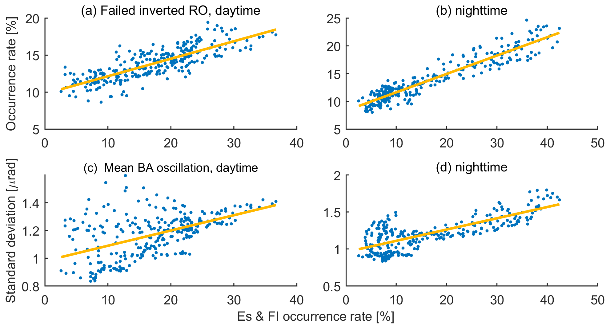
Figure 5Correlations between the ionospheric irregularity and the two parameters at middle and low latitudes (60∘ S–60∘ N) during the daytime (06:00–18:00 MLT, a, c) and nighttime (00:00–06:00 & 18:00–24:00 MLT, b, d) of 2011–2013. The yellow line is the corresponding linear least square fitting results.
For a better display of the high-latitude results, we plotted the irregularity and failed inverted RO occurrence rates as well as the bending angle oscillation variation with MLT–MLat in northern and southern polar regions in Fig. 4. As depicted in the left two panels, the ionospheric irregularity mainly occurs during 18:00–24:00 MLT, with occurrence peaks existing in aurora regions around midnight and moving toward the polar cap regions when approaching sunset. Values of the irregularity occurrence rate are around 10 %–20 % during the nighttime and can reach 30 % for peak regions. The middle two panels show the occurrence rate of failed inverted RO events. It is depicted that the peaks are located in aurora regions and extend to the polar cap regions from sunset to midnight. The increase in the occurrence rate around these regions might be affected by the high occurrence rate of Es. The failed inverted RO occurrence rates are also higher during the daytime in both hemispheres although the irregularity occurrence rates are lower than 10 % during this period. The right panels show the bending angle oscillation results. Its value is larger in aurora regions around midnight, which can reach 2.1 µrad. For those values in the Southern Hemisphere, strong bending angle oscillation can be seen in the polar cap regions during both the daytime and nighttime. In addition, the peak regions are located mainly between 80–90∘ S instead of 70–80∘ S as the irregularity occurrence peak shown in the bottom middle panel.

Figure 6Global geographical distribution of the Es and F layer irregularity occurrence rate (a–c), the failed inverted RO occurrence rate (d–f), and the mean bending angle oscillation (g–i) for equinox (a, d, g), northern summer (b, e, h), and northern winter (c, f, i).
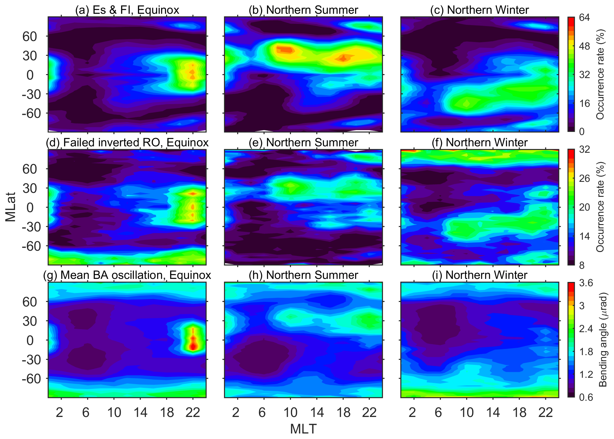
Figure 7The same as Fig. 6, but for geomagnetic local time (MLT) and geomagnetic latitude (MLat) variation.
We also use a scatter plot to study correlations between the ionospheric irregularity and the two parameters. The results are plotted in Fig. 5. Considering that the patterns of the failed inverted RO occurrence rate and the bending angle oscillation did not agree very well with those of the irregularity in high latitude regions, we mainly pay attention to the results at low and middle latitudes (60∘ S–60∘ N). Correlations during the daytime (06:00–18:00 MLT) and the nighttime (00:00–06:00, 18:00–24:00 MLT) were displayed, respectively. Overall, the correlations between the ionospheric irregularity and the two parameters are significant although they are not strictly linear especially for the bending angle oscillation during the daytime. The scatters in the panels are probably due to the fact that the failed inverted RO and the bending angle oscillation are not only affected by the Es and FI but also related to other factors. For example, the sudden stratospheric warming events can make the atmospheric structure changes significant and far from the climatology. As a result, bias between the RO observation and the climatological model could be increased and lead to the atmosphere RO event identified as “Bad” during inversion. Considering that the sudden stratospheric warming events often occur over the polar winter (Butler et al., 2015), they could also contribute to the pattern difference between the ionospheric irregularity occurrence rate and the two parameters in Fig. 4. Meanwhile, the observation and inversion noise could also make contributions.
In Figs. 3–5, we mainly pay attention to the yearly variation of the three parameters. As stated above, the seasonal variation of irregularity has been confirmed by previous studies (Arras et al., 2008; Chen and Huang, 2017). So the seasonal dependency of the failed inverted RO event and the bending angle oscillation could also exist. To investigate further, the occurrence rate variation with Lon–Lat and MLT–MLat were depicted in Figs. 6 and 7, respectively. Equinox (March, April, September, and October), northern summer (May, June, July, and August), and northern winter (January, February, November, and December) are considered here. Generally, in Fig. 6, the distributions of the failed inverted RO event occurrence are in good agreement with those of the irregularity. Both parameters are larger within ±30∘ in equinox and larger in summer than in winter. For northern summer, the occurrence peaks are near the North Africa and East Asia areas. For northern winter, the peaks are available in the Pacific Ocean regions nearby South America. Similar to the average pattern in Fig. 3, the failed inverted RO occurrence rate is high in polar regions even though the Es and FI occurrence is not obvious in comparison with those of peak regions at low latitudes. The MLT–MLat distributions of the irregularity and the failed inverted RO in Fig. 7 also show similar seasonal variations. But for the southern polar region in equinox and the northern polar region in northern winter, the failed inverted RO has significantly low occurrence rates of the ionospheric irregularity. For the bending angle results in both bottom panels in Figs. 6 and 7, it is apparent that the bending angle oscillation value also follows a similar seasonal variation with the ionospheric irregularity occurrence, which is larger in summer than in winter with the equinox as the transitory season. It is noticeable that for the geographic distribution, larger values exist around northern Antarctica in all seasons. For the geomagnetic distributions, the three peaks along geomagnetic latitudes are available in all seasons.
In this paper, we focus on the ionospheric irregularity effects on GNSS atmospheric RO. The failed inverted RO events and the bending angle oscillation are the two main parameters we studied. The COSMIC S4 index provided by CDAAC during 2011–2013 is used to characterize the ionospheric irregularity occurrence rate such as the Es and the F region irregularity. The “bad” attribute in the atmPrf file is used to identify the failed inverted RO events on the condition that its value equals 1. The mean bending angle oscillation also from the atmPrf file is used to reflect the degree of bending angle oscillation. Results from single cases are analyzed first. Then the distribution patterns and seasonal variations of the ionospheric irregularity occurrence rate, failed inverted RO event occurrence rate, and the bending angle oscillation are presented for the correlation study. The main conclusions and implications of the paper are summarized as follows:
-
The ionospheric irregularity such as the Es and the F region irregularity could affect the GNSS atmospheric RO in terms of causing failed inverted RO events and the bending angle oscillation in both cases and statistically.
-
At middle and low latitudes during the daytime, both the failed inverted RO event and the bending angle oscillation are mainly affected by the Es. During the nighttime, the F region irregularity contributes to the obvious increases of the failed inverted RO occurrence rate and the bending angle oscillation around the geomagnetic equatorial regions.
-
In the polar regions, the Es mainly affect the two parameters in the aurora regions from sunset to midnight. But the correlations between the ionospheric irregularity and the two parameters are not as obvious as those at middle and low latitudes.
-
Seasonal dependency of the failed inverted RO occurrence and the bending angle oscillation exists, which also agree well with the seasonal variation of the Es and the F region irregularity.
-
The occurrence rate of the failed inverted RO can reach 15 % at low latitudes and even 20 % in peak regions. It means that hundreds of COSMIC RO events per day will be ruled out during quality control. The bending angle oscillation between 60 and 80 km also varies from ∼0.6 in trough regions to ∼2.5 µrad in peak regions. Although 60–80 km is not the main altitude range of RO data, the small-scale effects in atmospheric RO exist in all altitudes and could affect the atmospheric research related to RO products. Awareness of the ionospheric irregularity effect on RO could be beneficial to improve the data retrieval, quality control of GNSS atmospheric RO data processing, and data assimilation application in numerical weather prediction (Cardinali and Healy, 2014).
Overall, the ionospheric irregularity effects on GNSS atmospheric RO measurement exist. The effects can lead to the failed inverted RO event and the bending angle oscillation. A suitable filter may be effective in calibrating these effects and improving the quality of atmospheric RO products. We hope to investigate the potential calibrating method in our further work.
The code used to read the COSMIC file is available upon request.
All the COSMIC data used for this study are publicly available through the COSMIC Data Analysis and Archive Center (CDAAC) website (https://doi.org/10.5065/ZD80-KD74 (COSMIC Data Analysis and Archive Center (CDAAC), 2013) (last access: 17 April 2021).
ML and XY contributed to the study conceptualization. ML contributed to the statistical analysis and wrote the original draft. ML and XY reviewed and edited the manuscript.
The authors declare that they have no conflict of interest.
The University Corporation for Atmospheric Research (UCAR) COSMIC Data Analysis and Archive Center (CDAAC) is appreciated for processing and sharing the COSMIC radio occultation data to the community over years.
This research has been supported by the B-type Strategic Priority Program of the Chinese Academy of Sciences (grant no. Grant No. XDB41000000), the Open Research Project of Large Research Infrastructures (“Study on the interaction between low/mid-latitude atmosphere and ionosphere based on the Chinese Meridian Project”), the National Natural Science Foundation of China (grant no. 41427901), and the Key Research Program of the IGGCAS (grant no. Grant No. IGGCAS-201904).
This paper was edited by Peter Alexander and reviewed by two anonymous referees.
Angling, M. J., Elvidge, S., and Healy, S. B.: Improved model for correcting the ionospheric impact on bending angle in radio occultation measurements, Atmos. Meas. Tech., 11, 2213–2224, https://doi.org/10.5194/amt-11-2213-2018, 2018.
Anthes, R. A., Bernhardt, P. A., Chen, Y., Cucurull, L., Dymond, K. F., Ector, D., Healy, S. B., Ho, S. P., Hunt, D. C., Kuo, Y. H., Liu, H., Manning, K., McCormick, C., Meehan, T. K., Randel, W. J., Rocken, C., Schreiner, W. S., Sokolovskiy, S. V., Syndergaard, S., Thompson, D. C., Trenberth, K. E., Wee, T. K., Yen, N. L., and Zeng, Z.: The COSMIC/FORMOSAT-3 mission: Early results, B. Am. Meteorol. Soc., 89, 313–333, https://doi.org/10.1175/BAMS-89-3-313, 2008.
Arras, C., Wickert, J., Beyerle, G., Heise, S., Schmidt, T., and Jacobi, C.: A global climatology of ionospheric irregularities derived from GPS radio occultation, Geophys. Res. Lett., 35, L14809, https://doi.org/10.1029/2008gl034158, 2008.
Arras, C., Jacobi, C., and Wickert, J.: Semidiurnal tidal signature in sporadic E occurrence rates derived from GPS radio occultation measurements at higher midlatitudes, Ann. Geophys., 27, 2555–2563, 2009.
Axford, W. I.: The formation and vertical movement of dense ionized layers in the ionosphere due to neutral wind shears, J. Geophys. Res., 68, 769–779, https://doi.org/10.1029/JZ068i003p00769, 1963.
Beyerle, G., Schmidt, T., Michalak, G., Heise, S., Wickert, J., and Reigber, C.: GPS radio occultation with GRACE: Atmospheric profiling utilizing the zero difference technique, Geophys. Res. Lett., 32, L13806, https://doi.org/10.1029/2005gl023109, 2005.
Brahmanandam, P. S., Uma, G., Liu, J. Y., Chu, Y. H., Latha Devi, N. S. M. P., and Kakinami, Y.: Global S4 index variations observed using FORMOSAT-3/COSMIC GPS RO technique during a solar minimum year, J. Geophys. Res.-Space, 117, A09322, https://doi.org/10.1029/2012ja017966, 2012.
Butler, A. H., Seidel, D. J., Hardiman, S. C., Butchart, N., Birner, T., and Match, A.: Defining sudden stratospheric warmings, B. Am. Meteorol. Soc., 96, 1913–1928, https://doi.org/10.1175/BAMS-D-13-00173.1, 2015.
Cardinali, C. and Healy, S.: Impact of GPS radio occultation measurements in the ECMWF system using adjoint-based diagnostics, Q. J. Roy. Meteor. Soc., 140, 2315–2320, https://doi.org/10.1002/qj.2300, 2014.
Carter, B. A., Zhang, K., Norman, R., Kumar, V. V., and Kumar, S.: On the occurrence of equatorial F-region irregularities during solar minimum using radio occultation measurements, J. Geophys. Res.-Space, 118, 892–904, https://doi.org/10.1002/jgra.50089, 2013.
Chen, S. and Huang, Z.: Ionospheric F-layer global scintillation index variation using COSMIC during the period of 2007–2013, GPS Solutions, 21, 1049–1058, https://doi.org/10.1007/s10291-016-0593-2, 2017.
Chu, Y. H., Wang, C. Y., Wu, K. H., Chen, K. T., Tzeng, K. J., Su, C. L., Feng, W., and Plane, J. M. C.: Morphology of sporadic E layer retrieved from COSMIC GPS radio occultation measurements: Wind shear theory examination, J. Geophys. Res.-Space, 119, 2117–2136, https://doi.org/10.1002/2013ja019437, 2014.
COSMIC Data Analysis and Archive Center (CDAAC): COSMIC-1 data, UCAR Community Programs, https://doi.org/10.5065/ZD80-KD74, 2013.
Dungey, J. W.: Convective diffusion in the equatorial F region, J. Atmos. Terr. Phys., 9, 304–310, https://doi.org/10.1016/0021-9169(56)90148-9, 1956.
Danzer, J., Scherllin-Pirscher, B., and Foelsche, U.: Systematic residual ionospheric errors in radio occultation data and a potential way to minimize them, Atmos. Meas. Tech., 6, 2169–2179, https://doi.org/10.5194/amt-6-2169-2013, 2013.
Danzer, J., Healy, S. B., and Culverwell, I. D.: A simulation study with a new residual ionospheric error model for GPS radio occultation climatologies, Atmos. Meas. Tech., 8, 3395–3404, https://doi.org/10.5194/amt-8-3395-2015, 2015.
Danzer, J., Schwaerz, M., Kirchengast, G., and Healy, S. B.: Sensitivity analysis and impact of the kappa-correction of residual ionospheric biases on radio occultation climatologies, Earth and Space Science, 7, e2019EA000942, https://doi.org/10.1029/2019EA000942, 2020.
Fejer, B. G. and Kelley, M. C.: Ionospheric irregularities, Rev. Geophys., 18, 401–454, https://doi.org/10.1029/RG018i002p00401, 1980.
Healy, S. B. and Culverwell, I. D.: A modification to the standard ionospheric correction method used in GPS radio occultation, Atmos. Meas. Tech., 8, 3385–3393, https://doi.org/10.5194/amt-8-3385-2015, 2015.
Hocke, K., Igarashi, K., Nakamura, M., Wilkinson, P., Wu, J., Pavelyev, A., and Wickert, J.: Global sounding of sporadic E layers by the GPS/MET radio occultation experiment, J. Atmos. Sol.-Terr. Phy., 63, 1973–1980, 2001.
Li, G., Ning, B., Abdu, M. A., Yue, X., Liu, L., Wan, W., and Hu, L.: On the occurrence of postmidnight equatorial Fregion irregularities during the June solstice, J. Geophys. Res.-Space, 116, A04318, https://doi.org/10.1029/2010ja016056, 2011.
Li, M., Yue, X., Wan, W., and Schreiner, W. S.: Characterizing Ionospheric Effect on GNSS Radio Occultation Atmospheric Bending Angle, J. Geophys. Res.-Space, 125, e2019JA027471, doi.org/10.1029/2019JA027471, 2020.
Liu, C., Kirchengast, G., Sun, Y., Zhang, K., Norman, R., Schwaerz, M., Bai, W., Du, Q., and Li, Y.: Analysis of ionospheric structure influences on residual ionospheric errors in GNSS radio occultation bending angles based on ray tracing simulations, Atmos. Meas. Tech., 11, 2427–2440, https://doi.org/10.5194/amt-11-2427-2018, 2018.
Liu, C., Kirchengast, G., Syndergaard, S., Schwaerz, M., Danzer, J., and Sun, Y.: New Higher-Order Correction of GNSS RO Bending Angles Accounting for Ionospheric Asymmetry: Evaluation of Performance and Added Value, Remote Sensing, 12, 3637, doi.org/10.3390/rs12213637, 2020.
Mannucci, A. J., Ao, C. O., Pi, X., and Iijima, B. A.: The impact of large scale ionospheric structure on radio occultation retrievals, Atmos. Meas. Tech., 4, 2837–2850, https://doi.org/10.5194/amt-4-2837-2011, 2011.
Mao, T., Sun, L., Yang, G., Yue, X., Yu, T., Huang, C., Zeng, Z., Wang, Y., and Wang, J.: First Ionospheric Radio-Occultation Measurements From GNSS Occultation Sounder on the Chinese Feng-Yun 3C Satellite, IEEE T. Geosci. Remote, 54, 5044–5053, https://doi.org/10.1109/TGRS.2016.2546978, 2016.
Schreiner, W., Rocken, C., Sokolovskiy, S., Syndergaard, S., and Hunt, D.: Estimates of the precision of GPS radio occultations from the COSMIC/FORMOSAT-3 mission, Geophys. Res. Lett., 34, L04808, https://doi.org/10.1029/2006gl027557, 2007.
Schreiner, W., Sokolovskiy, S., Hunt, D., Rocken, C., and Kuo, Y.-H.: Analysis of GPS radio occultation data from the FORMOSAT-3/COSMIC and Metop/GRAS missions at CDAAC, Atmos. Meas. Tech., 4, 2255–2272, https://doi.org/10.5194/amt-4-2255-2011, 2011.
Straus, P. R., Anderson, P. C., and Danaher, J. E.: GPS occultation sensor observations of ionospheric scintillation, Geophys. Res. Lett., 30, 1436, https://doi.org/10.1029/2002gl016503, 2003.
Vorob'ev, V. V. and Krasil'nikova, T. G.: Estimation of the accuracy of the atmospheric refractive index recovery from Doppler shift measurements at frequencies used in the NAVSTAR system, USSR, Atmospheric and Oceanic Physics, English Translation, 29, 602–609, 1994.
Wickert, J., Marquardt, C., Beyerle, G., Reigber, C., and König, R.: Atmosphere sounding by GPS radio occultation: First results from CHAMP, Geophys. Res. Lett., 28, 3263–3266, doi.org/10.1029/2001gl013117, 2001.
Wu, D. L.: Sporadic E morphology from GPS-CHAMP radio occultation, J. Geophys. Res., 110, A01306, https://doi.org/10.1029/2004ja010701, 2005.
Wu, D. L.: Ionospheric S4 Scintillations from GNSS Radio Occultation (RO) at Slant Path, Remote Sensing, 12, 2373, https://doi.org/10.3390/rs12152373, 2020.
Yue, X., Schreiner, W. S., Zeng, Z., Kuo, Y.-H., and Xue, X.: Case study on complex sporadic E layers observed by GPS radio occultations, Atmos. Meas. Tech., 8, 225–236, https://doi.org/10.5194/amt-8-225-2015, 2015.
Yue, X., Schreiner, W. S., Pedatella, N. M., and Kuo, Y. H.: Characterizing GPS radio occultation loss of lock due to ionospheric weather, Space Weather, 14, 285–299, https://doi.org/10.1002/2015sw001340, 2016.
Zeng, Z. and Sokolovskiy, S.: Effect of sporadic E clouds on GPS radio occultation signals, Geophys. Res. Lett., 37, L18817, https://doi.org/10.1029/2010gl044561, 2010.