PHIPS-HALO: the airborne Particle Habit Imaging and Polar Scattering probe – Part 3: Single-particle phase discrimination and particle size distribution based on the angular-scattering function

A major challenge for in situ observations in mixed-phase clouds remains the phase discrimination and sizing of cloud hydrometeors. In this work, we present a new method for determining the phase of individual cloud hydrometeors based on their angular-light-scattering behavior employed by the PHIPS (Particle Habit Imaging and Polar Scattering) airborne cloud probe. The phase discrimination algorithm is based on the difference of distinct features in the angular-scattering function of spherical and aspherical particles. The algorithm is calibrated and evaluated using a large data set gathered during two in situ aircraft campaigns in the Arctic and Southern Ocean. Comparison of the algorithm with manually classified particles showed that we can confidently discriminate between spherical and aspherical particles with a 98 % accuracy. Furthermore, we present a method for deriving particle size distributions based on single-particle angular-scattering data for particles in a size range from 100 µm ≤ D ≤ 700 µm and 20 µm ≤ D ≤ 700 µm for droplets and ice particles, respectively. The functionality of these methods is demonstrated in three representative case studies.

1 Introduction

Mixed-phase clouds, consisting of both supercooled liquid droplets and ice particles, play a major role in the life cycle of clouds and the radiative balance of the earth (e.g., Korolev et al., 2017). Mixed-phase cloud processes are still rather poorly understood and represent a great source of uncertainty for climate predictions (e.g., McCoy et al., 2016). As a consequence, more in situ observations are needed to better understand mixed-phase cloud processes and improve climate models. Microphysical properties and the life cycle of mixed-phase clouds are strongly dependent on the phase separation of liquid and ice phases (e.g., Korolev et al., 2017). Furthermore, the radiative properties of cloud particles depend on their phase, shape and size. Despite the importance of mixed-phase cloud phase composition, a major uncertainty remains in the correct phase discrimination of cloud hydrometeors.

Currently, phase discrimination of individual cloud particles larger than 200 µm is based on circularity analysis (e.g.,  diameter or area ratio, Cober et al., 2001) of ice particle images measured by optical array probes such as the 2D-S and 2D-C (two-dimensional stereo probe and two-dimensional cloud probe, SPEC Inc., Boulder, CO, USA) or CIP (Cloud Imaging Probe, DMT, Longmont, CO, USA). For smaller particles, such discrimination methods of optical array probes are limited due to their optical resolution, especially for out-of-focus particles (Korolev, 2007). Instruments utilizing optical microscopy, such as the Cloud Particle Imager (CPI, SPEC Inc., Boulder, CO, USA), have a finer resolution and are able to discriminate particles down to 35 µm (McFarquhar et al., 2013). Still, the phase discrimination between droplets and quasi-spherical or small irregular ice particles based on their images can be challenging, as shown in Fig. 1.

For very small particles below D ≤ 50 µm, the SID family of instruments like the Small Ice Detector mark 3 (SID-3, Vochezer et al., 2016) and Particle Phase Discriminator (PPD, Hirst and Kaye, 1996; Kaye et al., 2008; Vochezer et al., 2016,; Mahrt et al., 2019) offer reliable phase discrimination based on the spatial distribution of the forward scattered light. The SID family of instruments has the disadvantage, however, of not measuring the phase of each single particle but only for a sub-sample. Therefore, a large sampling time is required to derive ice concentrations in mixed-phase clouds that are dominated by droplets. The Cloud and Aerosol Spectrometer with Polarization (CAS-POL, DMT, Longmont, CO, USA, Glen and Brooks, 2013) is an instrument that measures the light scattered by single cloud particles and aerosols in a size range of 0.6 µm ≤ D ≤ 50 µm in the forward and backward directions. Based on the polarization ratio of the backscattered light, the sphericity of the cloud particles can be determined (Sassen, 1991; Nichman et al., 2016). However, recent studies have suggested that particle phase discrimination of polarization-based measurements can misclassify up to 80 % of the ice particles as droplets in the presence of small, quasi-spherical ice (Järvinen et al., 2016).

Hence, in the size range D ≤ 100 µm, methods for reliable particle phase discrimination are still needed. The Particle Habit Imaging and Polar Scattering probe (PHIPS) is a unique instrument designed to investigate the microphysical and light-scattering properties of cloud particles. It produces microscopic stereo images whilst simultaneously measuring the corresponding angular-scattering function from 18 to 170^∘ for single particles in a size range from 50 µm ≤ D ≤ 700 µm and 20 µm ≤ D ≤ 700 µm for droplets and ice particles, respectively. More information and a detailed characterization of the PHIPS setup and instrument properties can be found in Abdelmonem et al. (2016) and Schnaiter et al. (2018).

In this work, we will present a method to discriminate the phase of single cloud particles based on their angular-scattering function. An algorithm was developed using experimental in situ data from two aircraft campaigns targeting mixed-phase clouds. We present a method to use single-particle angular-light-scattering measurements to produce size distributions for spherical and aspherical particles separately.

This work is structured in the following: in Sect. 2, the aircraft campaigns of the experimental data sets used in this work are introduced. Next, in Sect. 3 the methodology and calibration of the phase discrimination algorithm are explained. In Sect. 4, the particle sizing will be introduced, and several methods for shattering correction will be discussed. Finally, in Sect. 5, the described methods will be used in three case studies. The results will be compared to measurements by other cloud particle probes during the same campaigns.

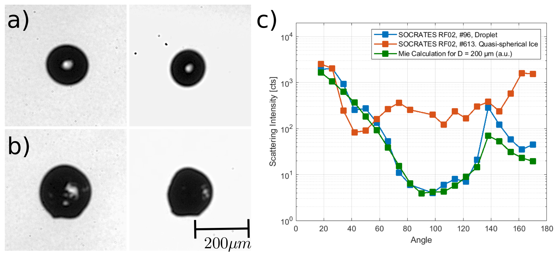
Figure 1 Stereo micrograph of a droplet (a) and a quasi-spherical ice particle (b) taken by the PHIPS probe. In the stereo micrograph, the two views of the particle have an angular distance of 120^∘. The instrument concurrently recorded the angular-light-scattering functions of the imaged particles as displayed in (c). The theoretical scattering function calculated for a droplet with a diameter of 200 µm calculated using the Mie theory is shown for comparison in (c). The calculated scattering intensity is integrated over the field of view of each of PHIPS' 20 polar nephelometer channels so it can be compared to the measurement (see Supplement Sect. S6 for details).

2 Experimental data sets

In this work, we use experimental in situ data gathered during two airborne field campaigns to develop and test a single-particle phase discrimination algorithm for the PHIPS probe. The two data sets refer to the two respective campaigns:

1. ACLOUD – Arctic CLoud Observations Using airborne measurements during polar Day of May–June 2017 based in Svalbard (Spitsbergen, Norway) and

2. SOCRATES – Southern Ocean Clouds, Radiation, Aerosol Transport Experimental Study of January–February 2018 based in Hobart (Tasmania, Australia).

An overview of the meteorological and microphysical conditions as well as the instrumentation during those campaigns can be found in Knudsen et al. (2018) and Wendisch et al. (2019) for ACLOUD and McFarquhar et al. (2019) for SOCRATES. The sampling during both campaigns includes a wide variety of different cloud conditions: warm clouds, supercooled liquid clouds, ice clouds and mixed-phase clouds. Clouds were sampled in an altitude range from boundary layer clouds below 200 m to mid-level clouds between 4000 and 6000 m. Temperatures ranged from −15 to +5 ^∘C during ACLOUD and −35 to +5 ^∘C during SOCRATES. The sampled ice particles covered a range of different particle shapes and habits (columns; plates; needles; bullet rosettes; dendrites; and irregulars, including rough, rimed and pristine particles) as well as sizes. More details can be found in the Supplement (Sect. S1). The instrumentation on the two aircraft included cloud particles probes such as the SID-3, CDP (Cloud Droplet Probe, DMT, Longmont, CO, USA), CIP and PIP (Precipitation Imaging Probe, DMT, Longmont, CO, USA) during ACLOUD and 2D-C, 2D-S and CDP during SOCRATES. Due to the variability of the meteorological conditions and sampled particles, the data gathered during these two campaigns make a suitable and representative data set to develop the phase discrimination and particle size distribution algorithms that are presented in this work.

3 Single-particle phase discrimination algorithm

The angular-scattering properties of spherical particles can be analytically calculated using the Mie theory. The angular-scattering properties of usually aspherical ice particles, however, are much more complex, which significantly alters their scattering properties compared to spherical particles (Järvinen et al., 2018; Schnaiter et al., 2018; Sun and Shine, 1994; Um and McFarquhar, 2011). Hence, it is possible to differentiate between the angular-scattering functions (ASFs) of spherical and aspherical particles by looking into differences in the angular-light-scattering behavior in the angular regions where spherical particles exhibit unique features, like the minimum around 90^∘ and the rainbow around 140^∘. In this section, we introduce four scattering features and develop an algorithm that is able to classify each particle based on the combined information from multiple features of the ASFs (see Fig. 2).

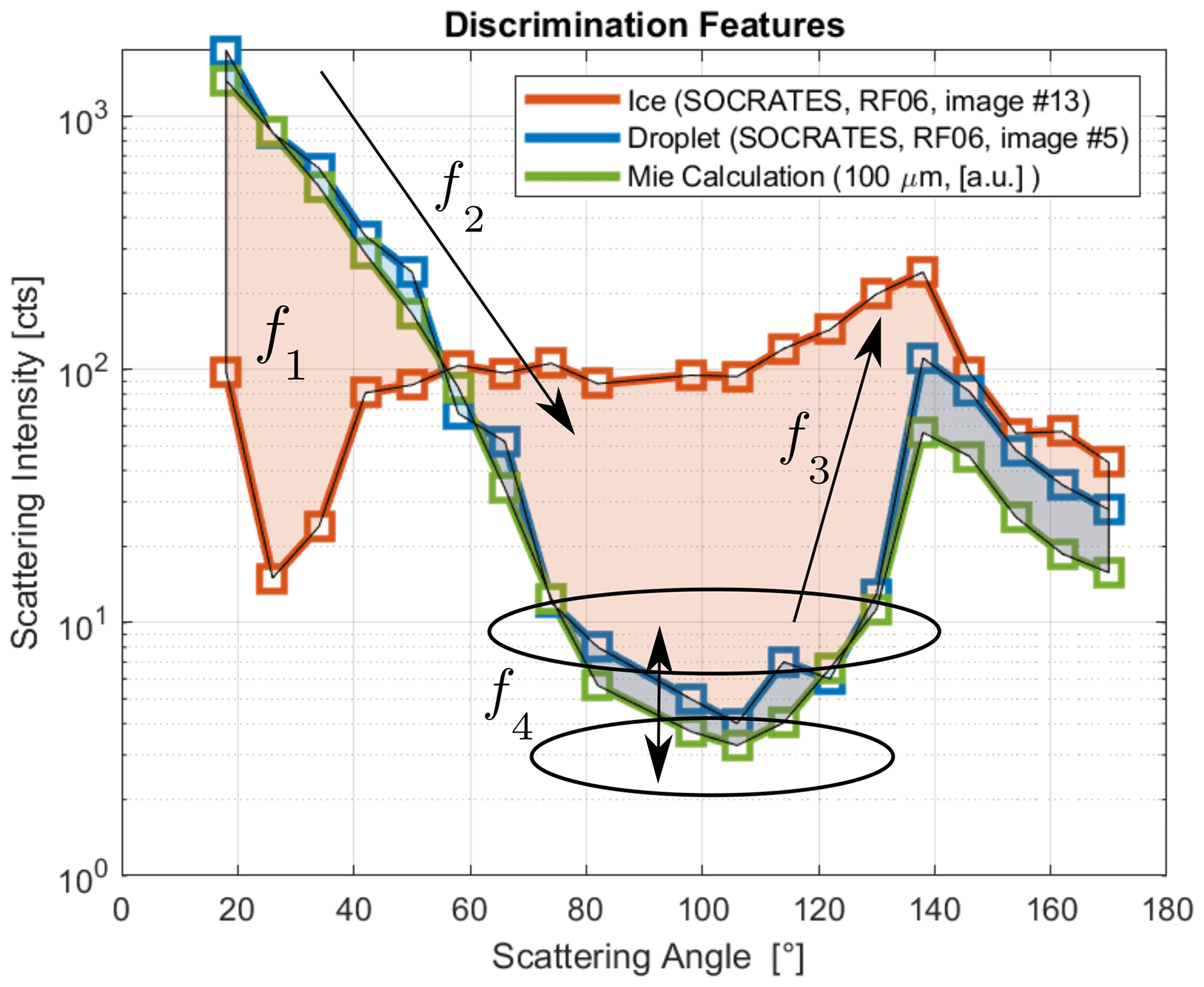
Figure 2 Visualization of the four classification features: f₁ is the Mie comparison (shaded area between curves and Mie calculation); f₂ is the downslope; f₃ is the upslope before the rainbow feature; and f₄ is the ratio around the minimum at 90^∘. The green line shows the calculated ASF for a theoretical spherical particle. The blue area and lines show the measured ASFs of an exemplary droplet (D = 119.6 µm) and ice crystal (D = 165.8 µm) from the SOCRATES campaign.

The basic concept of the development procedure for the single-particle phase discrimination algorithm will be explained in this section and is shown in Fig. 3. In the first step, ASFs calculated by the Mie theory (BHMIE, Bohren and Huffmann, 2007) for spherical particles using the refractive index for water (n_refr=1.332) are compared to modeled ASFs of aspherical ice crystals (Baum et al., 2011 and Yang et al., 2013). Based on the differences in the ASFs, typical features are determined that are characteristic for spherical or aspherical particles (see Fig. 2). The algorithm is then calibrated and validated using PHIPS data from the two field campaigns that were introduced in the previous section. This data set consists of about 23 000 representative single cloud particles of various phases, habits and sizes for which stereo micrographs as well as the corresponding ASFs are available. Those particles are manually classified as spherical or aspherical based on their appearance in the stereo micrographs. The calibration of the phase discrimination algorithm is then based on the ACLOUD data set only. This way, a classification probability for every feature is determined. The different features are then weighed and combined to a final discrimination probability for every single particle. Lastly, the data from the SOCRATES campaign are used to validate the discrimination algorithm and to determine the discrimination accuracy.

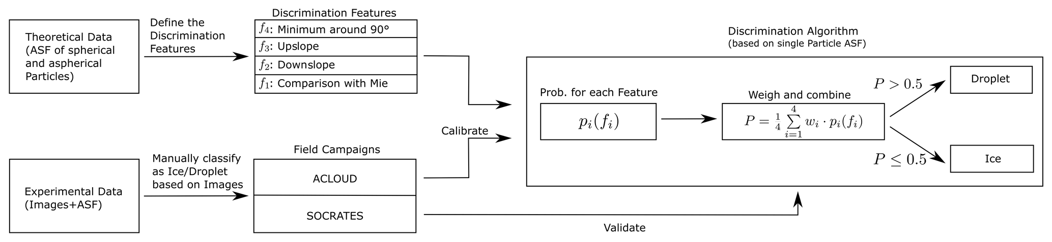
Figure 3 Schematics showing the basic working principle of the phase discrimination algorithm.

3.1 Discrimination features

3.1.1 f₁: comparison with Mie scattering

One approach to discriminate between spherical and aspherical particles is to compare a particle's ASF with theoretical Mie calculations. To estimate the deviation of the observed ASFs from the calculated Mie scattering, we evaluate the integrated difference between measurement and calculation (shaded area between the curves in Fig. 2). Figure 4 shows a step-by-step explanation of the determination of the f₁ parameter based on two exemplary droplets: a droplet (d1) with D = 119.6 µm (the same particle as used in Fig. 2) and a theoretical Mie sphere (d2) with D = 200 µm. Figure 4a shows the ASFs for the two particles as well as the ASF of the reference Mie sphere with D = 100 µm.

We define the ratio between the measured intensity I_exp of an individual particle and the Mie calculation I_Mie for a spherical reference particle with a diameter of 100 µm for every nephelometer angle θ_i of

$$\begin{array}{}\text{(1)}& {\displaystyle }q\left({\mathit{\theta }}_i\right)={\displaystyle \frac{I_{\text{exp}}\left({\mathit{\theta }}_i\right)}{I_{\text{Mie}}\left({\mathit{\theta }}_i\right)}}\end{array}$$

as shown in Fig. 4b. To be comparable to the measured intensities, the calculated theoretical Mie scattering function was integrated over the field of view of the polar nephelometer channels (see Sect. S6). Ideally, this ratio q_i should be calculated with a theoretical reference particle with the same diameter as the detected particle. However, the diameter of the measured particle is not known without applying a size calibration first. To circumvent this, each q_i is normalized by the median over all channels $\stackrel{\mathrm{‾}}{q}$ (dashed line in Fig. 4b). For a spherical particle, this ratio should be approximately q≃ const. (see Sect. S2). Since we do not know the diameter of the measured particle without applying a size calibration, q is normalized by the median over all channels $\stackrel{\mathrm{‾}}{q}$, and the influence of the approximately constant factor can be neglected. This also has the advantage that we do not need to calibrate the conversion factor from counts to power unit (W) of the photomultiplier array, which can change for different campaigns, gain settings and changes in laser power. Thus, the discrimination algorithm works for different campaigns and settings without further calibration.

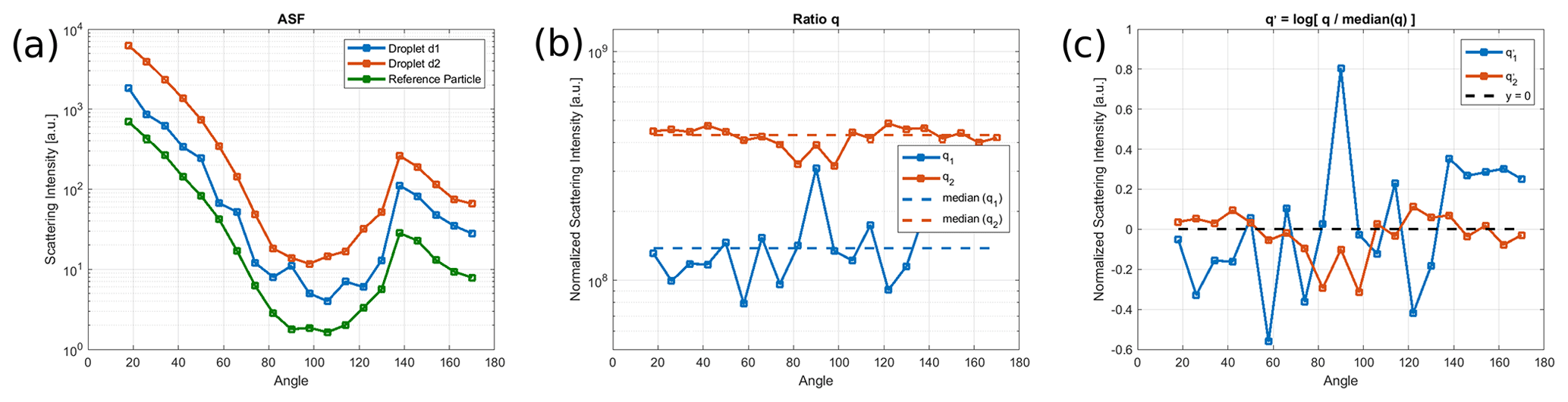
Figure 4 Determination of the feature parameter f₁ of two exemplary droplets: droplet d1 (blue) is the same particle as used in Fig. 2. Droplet d2 (red) is a theoretical Mie sphere with d = 200 µm. The plots show the particles' ASFs (a), q and $\stackrel{\mathrm{‾}}{q}$ (b) and q^′ (c). The resulting f₁ is then calculated as the integral over all channels (i.e., area between each curve and y = 0). The resulting values are f₁ = 3.7 for d1 and f₁ = 2.2 for d2.

Furthermore, as the deviation in “both directions” from the calculated Mie intensity has to be weighted equally, q_i=2 and $q_i=\frac{\mathrm{1}}{\mathrm{2}}$ should be equivalent. Therefore, we make the transformation $q_i^{\prime }\to \log (q_i/\stackrel{\mathrm{‾}}{q})$. The resulting “feature parameter” is then finally defined as the logarithm of the integral over all angles θ_i:

$$\begin{array}{}\text{(2)}& f_{\mathrm{1}}=log\left(\int \left|q_i^{\prime }\right|\mathrm{d}{\mathit{\theta }}_i\right)=\log \left(\int \left|\log \left({\displaystyle \frac{q_i}{\stackrel{\mathrm{‾}}{q}}}\right)\right|\mathrm{d}{\mathit{\theta }}_i\right),\end{array}$$

which corresponds to the area under the curves in Fig. 4c.

To demonstrate that this feature is representing a distinctive difference between spherical and aspherical particles, the distribution of the feature parameter value f₁ of representative, manually classified spherical and aspherical particles from the experimental in situ aircraft measurement campaigns introduced in Sect. 3.3 are shown in Fig. 6a. It can be seen that, roughly, if a given particle has a feature value of, e.g., f₁<4.5, it is likely spherical; if f₁>5, it has a high probability of being an aspherical particle. Phase discrimination based on this feature alone would already allow for a reasonable discrimination, but there also exist spherical particles with, e.g., f₁>5 that would be misclassified by using this approach. Hence, multiple features are taken into account to increase the discrimination accuracy.

3.1.2 f₂+f₃: down- and upslope

When looking at Fig. 2, the most distinctive differences between the ASFs of spherical and aspherical particles are the minimum around 90^∘ and the rainbow maximum around 140^∘ for spherical particles, whereas aspherical particles often show a flatter angular-scattering behavior. One way to extract those features is to evaluate the “exponential slope” of

$$\begin{array}{}\text{(3)}& f_{\mathrm{2}}={\displaystyle \frac{\log \left(I\right({\mathit{\theta }}_{\mathrm{2}}\left)\right)-\log \left(I\right({\mathit{\theta }}_{\mathrm{1}}\left)\right)}{{\mathit{\theta }}_{\mathrm{2}}-{\mathit{\theta }}_{\mathrm{1}}}}\end{array}$$

in the region before and after the minimum around 90^∘. This results in two features: the negative slope before the minimum and the positive slope between minimum and rainbow around 140^∘. In general, steeper slopes mean that a given particle is likely to be spherical. The first “slope feature” (f₂) is the “downslope”, which is simply the linear slope from ${\mathit{\theta }}_{\mathrm{1}}=\mathrm{42}{}^{\circ }$ to ${\mathit{\theta }}_{\mathrm{2}}=\mathrm{74}{}^{\circ }$. The first three scattering channels (θ=18, 26, 34^∘) are not taken into account here because they have a larger possibility of being saturated for larger particles. The slopes are determined by applying a linear fit to the logarithmic intensities in the channels between θ₁ and θ₂.

The second slope feature (f₃), the “upslope”, is calculated as the (logarithmic) slope from the minimum around 90^∘ to the maximum of the rainbow peak. Since the scattering intensity can be very low and, therefore, comparable to the magnitude of the background noise (especially for small particles), the “lower end” is averaged over multiple channels from $\mathit{\theta }=\mathrm{74}\text{to}\mathrm{106}{}^{\circ }$. The upper end of the slope is not fixed either but rather chosen dynamically, as the angular position of the rainbow peak can vary within four scattering channels between $\mathit{\theta }=\mathrm{130}\text{ and }\mathrm{154}{}^{\circ }$. Thus, we define the slope feature f₃ as

$$\begin{array}{}\text{(4)}& \begin{array}{rl}& f_{\mathrm{3}}\\ & ={\displaystyle \frac{\log \left(max\left[I\right(\mathrm{130}\text{ to }\mathrm{154}{}^{\circ }\left)\right]\right)-\log \left(\text{mean}\left[I\right(\mathrm{74}\text{ to }\mathrm{106}{}^{\circ }\left)\right]\right)}{{\mathit{\theta }}_{\mathrm{2}}-{\mathit{\theta }}_{\mathrm{1}}}},\end{array}\end{array}$$

with the corresponding angle of the rainbow maximum θ₂ and the minimum ${\mathit{\theta }}_{\mathrm{1}}=\mathrm{90}{}^{\circ }$. This way, even small particles and elongated particles with a shifted rainbow peak (see Sect. S4) can be classified correctly.

3.1.3 f₄: ratio around the 90^∘ minimum

Another possible way to depict the depth of the 90^∘ minimum is to directly compare the intensities in the vicinity around $\mathit{\theta }=\mathrm{90}{}^{\circ }$ with channels that are farther away (see Fig. 2). Hence, the “mid-ratio” feature is defined as

$$\begin{array}{}\text{(5)}& {\displaystyle }{f}_{\mathrm{4}}=\log \left({\displaystyle \frac{\text{mean}\left[I\right(\mathrm{58},\mathrm{66},\mathrm{114},\mathrm{122}{}^{\circ }\left)\right]}{\text{mean}\left[I\right(\mathrm{74},\mathrm{82},\mathrm{90},\mathrm{98},\mathrm{106}{}^{\circ }\left)\right]}}\right).\end{array}$$

With the distinct shape of the ASFs of droplets around the 90^∘ minimum one could argue that an intensity threshold might be enough to discriminate between spherical and aspherical particles (e.g., classifying every particle with $I(\mathit{\theta }=\mathrm{90}{}^{\circ })$ smaller than a certain threshold I_thresh as spherical). However, looking at absolute values would prove impractical, as the ASF scales with particle size: a very small aspherical particle could still fulfill $I(\mathit{\theta }=\mathrm{90}{}^{\circ })<I_{\text{thresh}}$ as well as a rather large spherical particle $I(\mathit{\theta }=\mathrm{90}{}^{\circ })>I_{\text{thresh}}$, respectively. Hence, the discrimination features presented here are all based on relative values, slopes and ratios instead of discrete thresholds. Further, all discrimination features are based on the scattering signal of multiple channels instead of only one channel to minimize the impact of noise. This allows for the discrimination algorithm to be used for multiple campaigns (even with differing settings or minor hardware changes or malfunction) without additional calibration (see Sect. 3.4).

3.2 Simulation of the feature parameters

To prove that the defined set of discrimination features reliably discriminates between spherical and aspherical particles, we calculate the feature parameter values f_i based on theoretical ASFs. For droplets, we use the Mie theory for spherical particles with diameters from 100 µm ≤ D ≤ 700 µm. For ice, we use modeled orientation-averaged ASFs of ice crystals of different habits and roughness using the databases from Baum et al. (2011) and Yang et al. (2013) in the size range from 20 µm ≤ D ≤ 700 µm. Similarly as explained beforehand, the scattering intensities are integrated over the field of view of the polar nephelometer channels. The distribution of feature parameters is shown in Fig. 5. It can be seen that the resulting values differ significantly for droplets and ice. This shows that the aforementioned features are in fact fit to discriminate the ASFs of spherical and aspherical particles. From now on, we will assume that particles that appear spherical in terms of their angular-light-scattering behavior are droplets and particles that appear aspherical in their ASFs are ice. Note that this includes also deformed droplets (as discussed in the Sect. S4) as well as quasi-spherical ice as shown in Fig. 1.

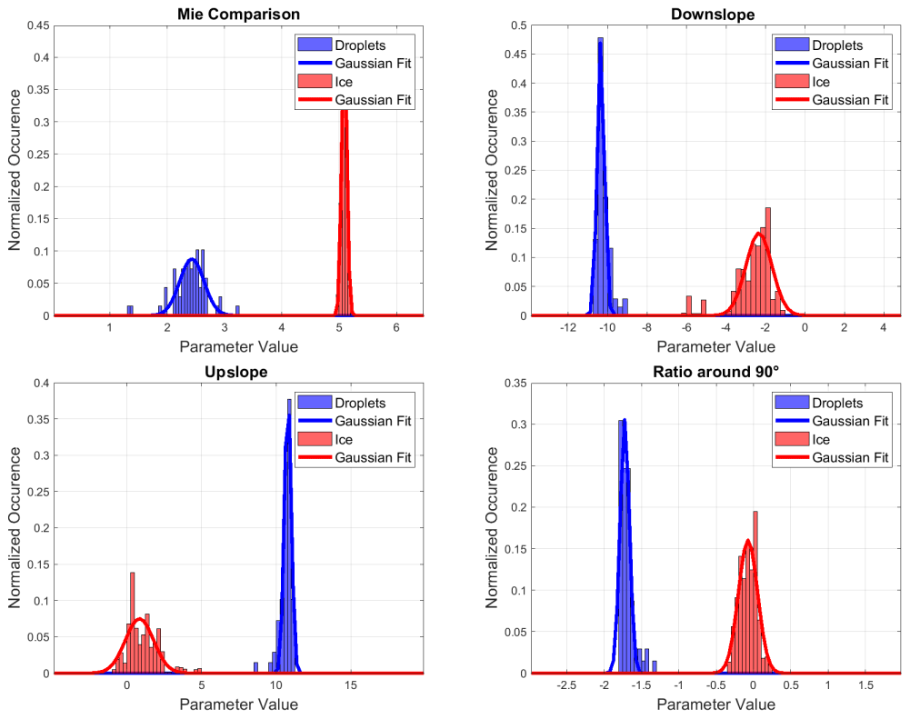
Figure 5 Normalized histograms of the discrimination features f_i evaluated for theoretical ASFs. Simulated ASFs were calculated using the Mie theory in the case of droplets (blue) and by selecting typical ice particle habits (red) from the light-scattering databases by Baum et al. (2011) and Yang et al. (2013). Normal distribution fits to the data are depicted by solid lines in the graphs. Note that the simulations provide orientation-averaged ASFs, whereas the observed particles by PHIPS have random but fixed orientations.

3.3 Calibration

Next, the discrimination features were applied to experimental data sets of real cloud particles. We used in situ data of representative, manually classified single particles to validate the calculated features. These experimental data were then used to calibrate the algorithm (i.e., the classification probability functions P_i(f_i) for every feature), in order to have a numerical function that calculates a classification probability for every feature of a given particle and later a combined probability that can be used to discriminate every single particle based on its phase.

The experimental data sets used for the calibration and verification of the discrimination algorithm are described in detail in Sect. 2. As it is the goal to develop an algorithm that is suitable without any further calibration for upcoming campaigns, the calibration and verification data sets are entirely disjunct: the ACLOUD data set is used for calibration; the verification is done using the SOCRATES data set. The ACLOUD and SOCRATES campaigns comprise 14 and 15 research flights, during which, in total about 41 000 and 235 000 single particles were detected by PHIPS, respectively. More details about sizes and habits of the manually classified particles used for the calibration can be found in the Supplement (Sect. S1). Because the imaging component of PHIPS has a limited temporal resolution, this results in about 22 000 and 32 000 events with matching stereo micrographs for the ACLOUD and SOCRATES flights, respectively. Based on these stereo micrographs, all imaged particles were manually classified as ice or droplets. To ensure a representative data set, only clearly distinguishable particles were taken into account, whereas images that show multiple particles and particles that are only partly imaged, out of focus or not clearly distinguishable were ignored. Hence, the resulting data set used for the calibration (based on the ACLOUD campaign) includes 1853 droplets and 7885 ice crystals. The data set used for the validation and determination of the discrimination accuracy (see Sect. 3.4) contains 2284 droplets and 9936 ice crystals from the SOCRATES campaign. The chosen data sets consist of representative cloud particles which cover a wide range of different particle shapes and habits (columns; plates; needles; bullet rosettes; dendrites; and irregulars, including rough, rimed and pristine particles) as well as sizes D=20–700 µm and D=100–700 µm for ice and droplets, respectively.

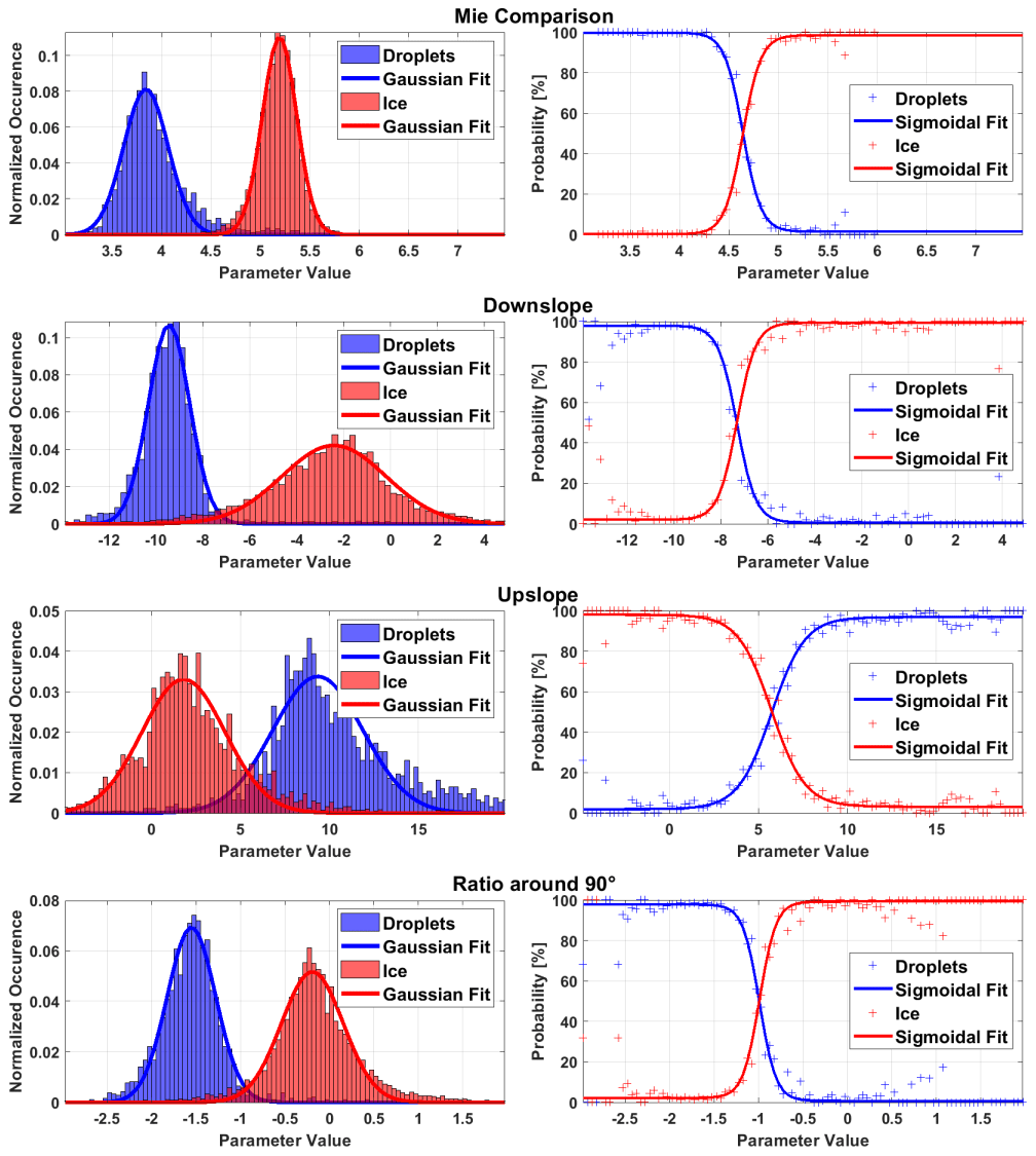
Figure 6 Left: normalized histograms of the discrimination features, f₁, f₂, f₃ and f₄, of all manually classified particles (blue: droplets, red: ice) from the ACLOUD campaign that were used for the calibration of the discrimination algorithm. The histograms can be nicely fitted by normal distributions (solid lines). Right: corresponding probability for a given particle with a given feature parameter value to be classified as ice or a droplet, including sigmoidal fits.

The left panels of Fig. 6 show, similar to the simulations in Fig. 5, the relative amount n(f_i) of particles that share a certain feature parameter value X. To account for the different amount of ice and droplets in the data set ($N_{\text{ice}}\approx \mathrm{3}\cdot N_{\text{droplet}}$), the number frequencies n_droplet/ice are normalized by the total amount of droplets and ice particles. The plots show that the distribution of the four aforementioned feature parameters are clearly distinct for droplets and ice and thus represent features that can be used to discriminate droplets from ice. Further, it can be seen that these normalized occurrences n(f_i) are normally distributed. The distributions of the four feature parameters based on the measurements (Fig. 6) show a similar trend to the simulations (Fig. 5). The width of the distributions of feature parameters for measurements is much broader compared to the simulations. This can be explained by the single orientation of the measured crystals compared to the orientation averaging that was used in the simulations. Orientation averaging tends to smooth out features in the ASFs and thus cause more narrow feature parameters. It should be also noted that the theoretical computations are for idealized crystals. Nevertheless, the mean values of the distributions agree very well. The only exception to this is the mean value of the distribution of droplets for f₁, which is shifted slightly to larger values compared to the simulations. This is to be expected because the “Mie comparison feature” f₁ is based on the relative difference between the measured and calculated ASFs. This difference is much smaller for simulated particles as discussed in Sect. 3.1.1.

However, Fig. 6 also shows that the ice and droplets modes are not always clearly separable for every feature and for every particle. Therefore, instead of using a sharp threshold, a classification probability of

$$\begin{array}{}\text{(6)}& {\displaystyle }{P}_i\left(f_i\right)={\displaystyle \frac{n_{\text{ice}}\left(f_i\right)}{n_{\text{ice}}\left(f_i\right)+n_{\text{droplet}}\left(f_i\right)}},\end{array}$$

where a particle is classified as ice (or with 1−P_i(f_i) as a droplet) based on the ratio between n_droplet(f_i) and n_ice(f_i) for each feature (see right panels of Fig. 6), is defined. Assuming that n_i(f_i) follows normal distributions with comparable widths, P_i(f_i) can be approximated and fitted by a sigmoid function. Following that, the probability functions P_i(f_i) are determined by using a sigmoidal fit for every feature based on the empiric data. These probabilities, P_i, for each feature are combined to

$$\begin{array}{}\text{(7)}& P_{\text{combined}}={\displaystyle \frac{\mathrm{1}}{n}}\sum _{i=\mathrm{1}}^n{w}_i\cdot P_i\left(f_i\right)\end{array}$$

with empiric weights w_i that are determined using recursive, linear optimization. Coincidentally, the optimum weight is to weigh all four features equally, i.e., $w_{\mathrm{1}}=w_{\mathrm{2}}=w_{\mathrm{3}}=w_{\mathrm{4}}=\mathrm{1}$ and thus P_combined=mean(P_i). Finally, this results in a classification probability for every given particle with a set of calculated feature parameter values $[f_{\mathrm{1}},f_{\mathrm{2}},f_{\mathrm{3}},f_{\mathrm{4}}]$, which is then classified based on P_combined as a droplet (P≤50 %) or ice particle (P>50 %). Details on the fit parameters for P_i can be found in Appendix A and Appendix B.

3.4 Discrimination accuracy

Discrimination algorithms often run in danger of “overtraining” or creating a “lookup table”, resulting in seemingly very good discrimination accuracies that, in reality, are just recreating the “training data” used for calibrating the system but fail to classify new, “unknown” data sets. In order to avoid this, the “training” and “test” data set are not only disjunct but also from entirely different field campaigns. Furthermore, this proves that the algorithm is able to function independently for different campaigns without further calibration.

The confusion matrices (Fawcett, 2006) for the discrimination algorithm for the two campaigns are shown in Fig. 7. For the SOCRATES data set, 99.7 % of ice particles could be correctly classified as ice, and only 29 out of 9936 were misclassified as droplets; 95.8 % of droplets were classified correctly, and 95 out of 2284 were misclassified as ice. In total, out of all particles, 99.0 % were classified correctly. Respectively, if a particle is classified as ice (droplet) by the algorithm, the expected error (i.e., the probability that the initial particle was actually a droplet) amounts to 0.9 % (1.3 %). Also, 100 % of the theoretical particles used in Sect. 3.2 (which were not used for the calibration) were classified correctly. More details about the discrimination accuracy and misclassified particles can be found in the Supplement.

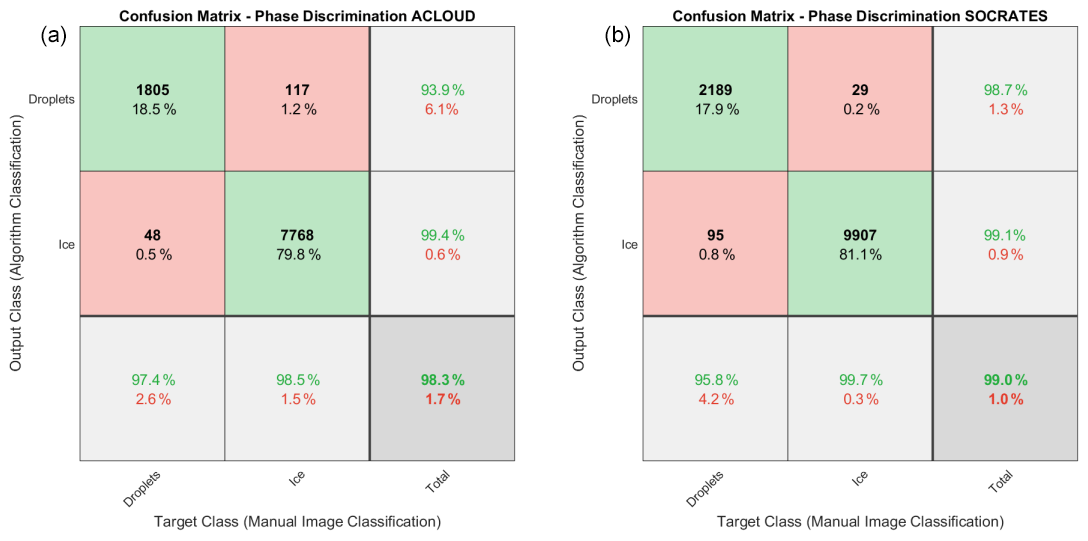
Figure 7 Confusion matrices that visualize the classification accuracy of the ice discrimination algorithm. The discrimination algorithm was applied to all manually classified particles from both the ACLOUD (a) and SOCRATES (b) data sets. In both cases the combined probability P_combined from the ACLOUD calibration was used to calculate the classification probability of each individual particle.

Note that during ACLOUD, one channel ($\mathit{\theta }=\mathrm{34}{}^{\circ }$) was malfunctioning and is hence excluded from the analysis. During SOCRATES, the $\mathit{\theta }=\mathrm{90}{}^{\circ }$ channel was observed to be affected by the background noise in the case of droplets and was thus excluded. However, due to the design of the discrimination features (i.e., averaging over multiple channels) the implications on the discrimination are reduced, and the same parameterization still works well for the SOCRATES data set.

3.5 Phase discrimination using machine learning

Binary classification problems like the one presented in this work are typically well fit to be solved using machine learning (ML) algorithms (Kumari and Srivastava, 2017). For example, in recent works, Mahrt et al. (2019) and Touloupas et al. (2020) have presented different methods to employ ML to discriminate ice and liquid cloud particles using the PPD-HS (High-speed Particle Phase Discriminator) and HOLIMO (HOLographic Imager for Microscopic Objects), respectively. Depending on the chosen classification problem, ML algorithms can be very easy and quick to set up: basically all one needs is a (pre-classified) training data set. There exists software, such as, e.g., TensorFlow (Google LLC, CA, USA), that is specialized on ML; however, nowadays most common analysis software such as, e.g., MATLAB or Mathematica has built-in ML toolboxes that make working with ML quite easy, fast and comfortable. In general, the main idea is basically that the ML algorithm is able to identify systematic differences and common features of the different “types” on its own (even such that could be hard to find for humans) and divide the data set accordingly. This way, the ML can classify even new, unknown data sets that “it has never seen” before. Given a large enough training data set, ML algorithms can achieve high discrimination accuracies.

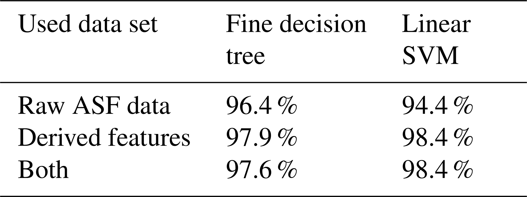
For comparison with the analytical approach used in this work, the classified data set was analyzed using two different, basic supervised ML methods, using (a) fine decision tree and (b) linear support-vector machine (SVM). This was done once for the raw data, i.e., just the scattering intensity of the 18 scattering channels (the θ=34 and $\mathit{\theta }=\mathrm{90}{}^{\circ }$ were removed) as well as using the four features $[f_{\mathrm{1}},f_{\mathrm{2}},f_{\mathrm{3}},f_{\mathrm{4}}]$ presented in this work and using both raw intensity and derived features. Again, the data were trained using the ACLOUD data set and tested against the SOCRATES data set. All particles that had any missing values were discarded. The corresponding discrimination accuracies are shown in Table 1. It can be seen that the different ML methods already show good results. Also, it shows once more that the presented features $[f_{\mathrm{1}},f_{\mathrm{2}},f_{\mathrm{3}},f_{\mathrm{4}}]$ are indeed fit to represent the difference in the ASFs. With more fine tuning, especially the discrimination accuracy of the SVM approach might reach the 99 % of the analytical approach.

Table 1 Classification accuracies for different ML approaches and different input information.

However, despite the discussed advantages, ML also has one main disadvantage: it is hard to understand what the algorithm is doing in detail. Basically, what you end up with is a black box that classifies input data with a given confidence, but you cannot tell why. Hence, it is very hard to analyze which features are relevant for the classification. Further, since the ML knows only statistics, not physics, it is possible that the ML algorithm links the classification to “un-physical parameters” that can introduce systematical biases. For example, it could be possible that the ML algorithm learns that large particles (with a corresponding high total scattering intensity) are typically ice, whereas droplets are typically smaller and hence scatter less light. Thus, it would look at the “amplitude” rather than the “shape” of the ASFs and classify all “large particles” as ice. Since the number of large droplets in the used data set is rather small, the overall discrimination accuracy would be quite high; however there would be the systematical bias that the few large droplets would tend to be misclassified.

Hence and because it yields better discrimination accuracy, for this work, it was chosen to go with the “analytical approach” instead of ML. Also, the presented method has the advantage, as discussed previously, that it works without calibration for further campaigns, even when single-scattering channels are malfunctioning (such as, e.g., the $\mathit{\theta }=\mathrm{34}{}^{\circ }$ channel during ACLOUD) or the laser power is changed (since it takes only the shape, not the amplitude, into account). Nevertheless, the presented analytical method works similar to the ML approach.

4 Particle size distribution

Since only a sub-sample of the PHIPS particle events produce a stereo micrograph (i.e., maximum imaging rate of 3 Hz in ACLOUD and SOCRATES), particle size distributions that are based on the analysis of the images can only be calculated with a limited statistics. Furthermore, particle sizing might be biased for particles with sizes smaller than 30 µm, due to the limited optical resolution of the PHIPS imaging system (Schnaiter et al., 2018). Hence, in the following section, particle sizing based on the single-particle ASFs is introduced. The calibration based on the stereo micrographs is done following a similar approach as the phase discrimination in the previous section.

In order to calculate a particle number size distribution (PSD) per volume from the single-particle sizing data, as shown in Fig. 9, the volume sampling rate of the instrument has to be known. This sampling rate is simply the product between the speed of the aircraft and the sensitive area A_sens of the trigger optics. The size of the sensitive area A_sens is determined using optical-engineering software. This is presented in Sect. 4.2.

Figure 8 Calibration of the PHIPS-integrated light-scattering intensity measurement, expressed by the partial scattering cross section ${\mathit{\sigma }}_{\text{scatt}}^{\text{partial}}$, against the geometric diameter $D_{\text{p}}^{\text{geom}}$ deduced from the concurrent stereo micrographs. Stereo micrographs from the SOCRATES data set were manually classified for droplets (a, b) and ice particles (c, d).

4.1 Particle sizing

The individual detector channels of the PHIPS nephelometer measure scattered-light intensity I(θ) of individual cloud particles that can be converted to a differential scattering cross section ${\mathit{\sigma }}_{\text{scatt}}^{\text{diff}}\left(\mathit{\theta }\right)$ as

$$\begin{array}{}\text{(8)}& {\displaystyle }{\mathit{\sigma }}_{\text{scatt}}^{\text{diff}}\left(\mathit{\theta }\right)=I\left(\mathit{\theta }\right)/I_{\text{inc}}\cdot \mathit{\pi }\cdot d_{\text{laser}}^{\mathrm{2}}/\mathrm{4},\end{array}$$

with I_inc and d_laser being the power and diameter of the incident laser beam, respectively. Note that I(θ) in Eq. (8) has to be corrected for possible background intensity due to stray light in the instrument as well as dark photon counts of the photomultiplier array. Integrating Eq. (8) over all nephelometer channels gives a partial scattering cross section ${\mathit{\sigma }}_{\text{scatt}}^{\text{partial}}$ of the particle as defined for the PHIPS measurement geometry of

$$\begin{array}{}\text{(9)}& {\mathit{\sigma }}_{\text{scatt}}^{\text{partial}}=\mathit{\pi }\cdot d_{\text{laser}}^{\mathrm{2}}/(\mathrm{4}\cdot I_{\text{inc}})\cdot \int I\left(\mathit{\theta }\right)\mathrm{d}\mathit{\theta }.\end{array}$$

For spherical particles, ${\mathit{\sigma }}_{\text{scatt}}^{\text{partial}}$ is approximately proportional to their geometrical cross section $\mathit{\pi }\cdot D_{\text{p}}^{\mathrm{2}}/\mathrm{4}$, with D_p the particle diameter. This is demonstrated in the Supplement using Mie calculations (Sect. S2). Assuming that this is valid not only for spherical droplets but also for aspherical ice particles, the scattering cross-section equivalent particle diameter $D_{\text{p}}^{\text{scatt}}$ can be deduced from the PHIPS intensity measurement I(θ) as

$$\begin{array}{}\text{(10)}& D_{\text{p}}^{\text{scatt}}=a\cdot {\left(\int I\left(\mathit{\theta }\right)\mathrm{d}\mathit{\theta }-c_{\text{BG}}\right)}^{\frac{\mathrm{1}}{\mathrm{2}}}.\end{array}$$

In Eq. (10), a is a calibration coefficient that describes the incident laser properties, the detection characteristics of the polar nephelometer (e.g., the photomultiplier gain settings) and the angular-light-scattering properties of the particle, and c_BG is the integrated background intensity. As already discussed in the previous section, ice and droplets have vastly differing angular-scattering characteristics, i.e., scattering cross sections ${\mathit{\sigma }}_{\text{scatt}}^{\text{diff}}\left(\mathit{\theta }\right)$. Hence, different a coefficients are needed, and the calibration is done separately for ice and droplets. The coefficient a is calibrated based on the geometric cross-section equivalent diameter $D_{\text{p}}^{\text{geom}}$ derived from the stereo micrographs. A correction for the slight size overestimation of the CTA 2 (camera telescope assembly) for small particles due to the lower magnification is applied (see Schnaiter et al., 2018). More details on PHIPS image analysis routines can be found in Schön et al. (2011).

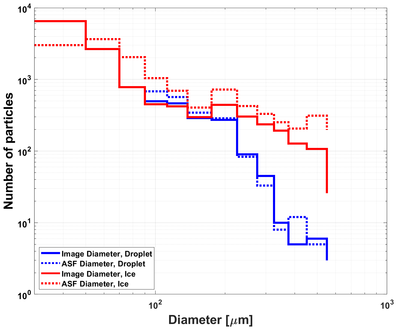
Figure 9 Comparison of PSD calculated from ASFs using the calibration defined in Eq. (10) (dotted line) and PSDs based on $D_{\text{p}}^{\text{geom}}$ derived from stereo micrographs (average of CTA1 and CTA2, solid line) for droplets (blue) and ice particles (red). The data are from all flights recorded during SOCRATES. Only stereo micrographs that showed only one completely imaged particle were taken into account. The same particles were used for both size distributions.

Similar to the calibration of the phase discrimination algorithm, manually classified imaged particles were used as a calibration data set. The data are binned with respect to the particle's geometrical area equivalent diameter. The bin edges are the same as used for the final PSD data product. Those are 20, 40, 60, 80, 100, 125, 150, 200, 250, 300, 350, 400, 500, 600 and 700 µm. For ice, the coefficient a is determined by fitting Eq. (10) through the median of each bin. For droplets, the function is fitted through all data points, since the data points are distributed over fewer size bins. The background intensity c_BG is determined as the integrated intensity from forced triggers averaged over time periods when no particles were present. c_BG is the same for droplets and ice. The calibration is performed for each campaign separately, assuming that the instrument parameters remain unchanged over the duration of one campaign. The resulting calibration of the scattering equivalent diameter for the SOCRATES campaign is shown in Fig. 8a and b for droplets and ice, respectively. The corresponding fit parameters are a_ice=1.4167 and a_droplet=1.4441. The background measurement value is c_BG=238.12.

Using this calibration Fig. 9 shows the comparison of the particle size distributions averaged over all flights of SOCRATES for both ice (red) and droplets (blue). It can be seen that the size distribution based on the images (solid lines) agrees well with the size distribution based on the angular-light-scattering functions (dotted lines).

Figure 10 Sensitive area based on FRED simulations for ice (red) and droplets (grey).

4.2 Sensitive area

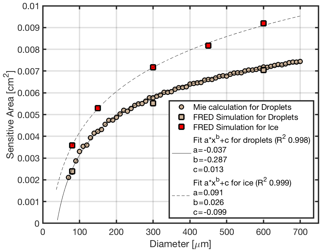
Due to the fact that the scattering laser of PHIPS has Gaussian intensity profiles and the field of view of the trigger optics shows gradual detection boundaries, A_sens is expected to be size dependent with a larger sensing area for larger particle sizes. Moreover, as (aspherical) ice particles usually have different differential scattering cross sections compared to (spherical) droplets, especially in side scattering directions where the trigger optics is located, A_sens is expected to be dependent also on the phase of the cloud particles. Therefore, we simulated the size dependence of A_sens for spherical and aspherical particles separately using the FRED Optical Engineering Software (Photon Engineering, LLC, USA), which combines light propagation by optical raytracing simulations with three-dimensional computer-aided design (CAD) visualization.

For the FRED simulations, the actual PHIPS trigger optics and three-dimensional laser intensity distribution were reconstructed in the three-dimensional CAD environment of the software resulting in the actual intensity field the particle is exposed to when penetrating the sensitive area of the instrument. Particles were step-wise positioned at different x, y and z position across the trigger field of view and depth of field to get a map of the scattered-light intensity that reaches the sensitive area of the trigger detector. Similar to the actual measurement, a threshold value for the simulated detector intensity was used that would trigger the system and, therefore, defines A_sens. This threshold was deduced by mapping the sensitive area of the instrument in the laboratory using a piezo-driven droplet dispenser which generates single 80 µm diameter water droplets (Schnaiter et al., 2018). Equating A_sens from the laboratory mapping with A_sens for the corresponding 80 µm FRED simulation then defined the threshold value that has to be used for all FRED simulations to calculate the size dependence A_sens.

The FRED simulations were performed for spherical particles with the refractive index of supercooled liquid water ($n=\mathrm{1.3362}+i\mathrm{1.82}\times {\mathrm{10}}^{-\mathrm{9}}$) and the three sizes of 80, 300 and 600 µm. The resulting A_sens are shown in Fig. 10 in grey color. Additionally, to validate the method, A_sens was also estimated using the Mie theory to calculate the differential scattering cross section for the trigger direction and multiply the results with the actual intensity field as defined by the FRED simulations. Although Mie calculations are faster to conduct, these calculations have the disadvantage that they assume a dimensionless particle, which induces uncertainties at the boundaries of the trigger field of view. Yet, the FRED simulations compare reasonably well with the results of the Mie calculations.

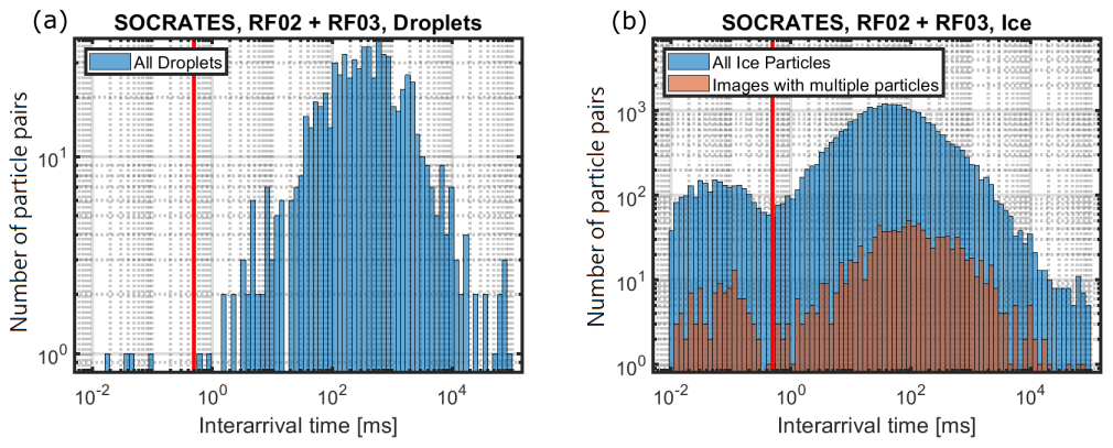
Figure 11 Histogram of interarrival times of ice particles (a) and droplets (b) measured during SOCRATES flights RF02 and RF03. Comparison of the interarrival times of all particles (blue) and only particles whose images were manually classified as shattering events (red). The red vertical line marks the τ≤0.5 ms threshold.

Ice particles were simulated roughened spheres whose surface light scattering was defined by the ABg model (Pfisterer, 2011). A refractive index of $n=\mathrm{1.3118}+i\mathrm{2.54}\times {\mathrm{10}}^{-\mathrm{9}}$ (Warren, 1984) was used for the ice simulations. The roughened ice sphere approach was chosen here to avoid computationally expensive orientation averaging, which was necessary in the case of using a non-spherical particle habit. The FRED simulations for ice particles were conducted for the five particle sizes of 80, 150, 300, 450 and 600 µm. As can be seen in Fig. 10, the A_sens values for ice are significantly larger than those for water droplets of the same diameter. An exponential function was fitted to the FRED results to get A_sens as a function of particle diameter. These functional dependencies are then used to calculate the volume sampling rate that is required to convert the single-particle data to particle size distributions.

4.3 Correction for shattering artifacts

One major source of uncertainty for wing-mounted probes is the shattering of ice particles on the instrument's outer mechanical structures or breakup of particles in the instrument inlet. An example of the shattering of a large particle and breaking up of aggregates in the inlet flow field can be found in the Supplement (Sect. S5). Shattering can lead to a significant overcounting of ice particles (e.g., up to a factor of 5 using a fast forward scattering spectrometer probe (FSSP), Field et al., 2003) and a bias in the particle size distribution towards smaller sizes. Here, we characterized the frequency of shattering events in the SOCRATES data set and present a method to detect shattering events within the PHIPS data sets. Even though the geometry of PHIPS was designed to minimize disturbances and turbulences in the instrument (e.g., sharp edges at the front of the inlet and an expanding diameter of the flow tube towards the detection volume; see Abdelmonem et al., 2016), shattering can still be an issue, especially in clouds where large cloud particles and aggregates with D>1 mm are present.

Since the field of view of the camera telescope assembly (CTA) is much larger (typically $\simeq \mathrm{1.5}\times \mathrm{1}$ mm) compared to the sensitive trigger area (see previous section), the stereo micrographs can be used to detect shattering events. However, as only a subset of detected particles is imaged, a shattering correction based on inspection of the stereo micrographs is not a practical and reliable solution. Still, manual examination of the stereo micrographs can be helpful to determine whether or not a cloud segment was affected by shattering in individual cases.

4.3.1 Interarrival time analysis

The most common method to detect shattering is based on the analysis of particle interarrival times (Field et al., 2003). If two (or more) particles are detected in very short succession, those particles are identified as shattering fragments and removed. Figure 11 shows a histogram of interarrival times (τ) of ice particles (left) and droplets (right) measured during two flights of SOCRATES. For ice, it is apparent that the otherwise approximately log-normal distributed interarrival times show a second, lower mode below τ≤0.5 ms (equivalent to spatial separation of ≤7.5 cm, assuming a relative air speed of $v=\mathrm{150}\text{m}{\text{s}}^{-\mathrm{1}}$) that is likely caused by shattering. For droplets, the second mode is not visible, since droplets tend to less fragment when entering the instrument inlet.

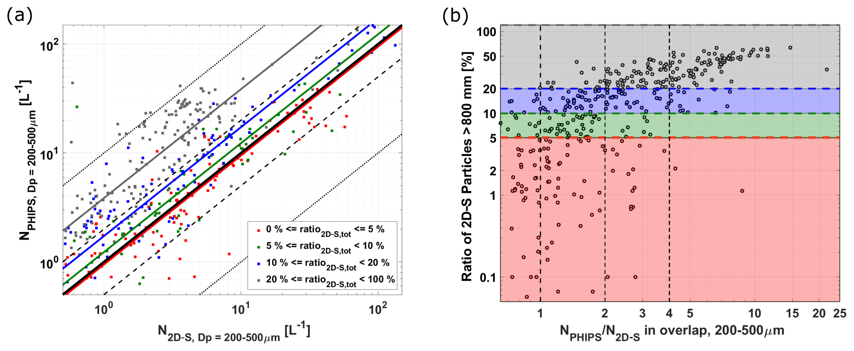
Figure 12 (a) Comparison of the total number concentrations of 2D-S and PHIPS. Each point is averaged over 30 s. The color code is based on the ratio of large 2D-S particles with D_max≥800 µm. The thick black line marks the 1:1 line; the dashed and dotted lines are a factor of 2 and 10. (b) Correlation of the ratio of number concentrations of PHIPS and 2D-S and the presence of large 2D-S particles. The horizontal line marks the 10 % threshold. The color code is the same as in (a).

Whereas the interarrival time analysis method is used in multiple optical array probes (2D-S and 2D-C, Field et al., 2003), the application is limited for single-particle instruments, like PHIPS, due to their small sensitive area. Near the detection volume, the inlet has a diameter of 32 mm, whereas the sensitive area measures only about 0.7 mm (depending on phase and size, as discussed in Sect. 4.2), which means that the probability of detecting two (or more) fragments of the same shattering event is very low. Furthermore, the instrument has a dead time of t=12 µs after each trigger event (Schnaiter et al., 2018). Shattering fragments that pass during this time are not detected. As shown in Fig. 11, only a small percentage of the particles whose images were manually classified as shattering (red) could be identified as shattering using the interarrival time analysis method. Hence it can be concluded that interarrival time analysis alone is not able to be a reliable shattering flag, either. Nevertheless, all particles with a low interarrival time τ≤0.5 ms are removed and excluded from the analysis. In the next section, a shattering flag is introduced that flags segments which are affected by particle shattering so they can be excluded from further analysis.

4.3.2 Shattering flag based on the presence of large particles

It is known that a particle's shattering probability is strongly size dependent. Large particles and aggregates are much more prone to shattering compared to small particles. To overcome the limitation of the interarrival time method to eliminate shattered particles, we introduce a shattering flag based on the presence of large particles. Figure 12a shows the total number concentration of particles in the size overlap region of PHIPS and 2D-S ($\mathrm{200}\mathrm{\mu }\mathrm{m}\le D\le \mathrm{500}\mathrm{\mu }\mathrm{m}$) for all SOCRATES flights. The data are averaged over 30 s segments. Only segments with $N_{\text{2D-S, overlap}}\ge \mathrm{0.5}{\text{L}}^{-\mathrm{1}}$ are taken into account. The color code indicates the fraction of 2D-S particles in the size range of D_max≥200 µm that are larger than 800 µm. The diagonal lines mark the median ratio between $N_{\text{PHIPS}}/N_{\text{2D-S}}$ of each color. Figure 12b shows the correlation of the difference between PHIPS and 2D-S in the overlap region and the ratio of large particles. It can be seen that the two probes agree very well in segments with only a few large particles.

In segments that consist of more than 10 % of large particles, PHIPS and 2D-S tend to disagree, and PHIPS can overestimate particle concentrations up to a factor >10. This can be explained by the shattering of large particles on the instrument inlet tip or wall or disaggregation of large aggregates due to shear forces in the inlet flow. Therefore, said marker for the presence of large particles will be used as a shattering flag to mark cloud segments that are potentially affected by shattering. In segments where the 2D-S did not detect any particles or was not measuring, for any reason, 2D-C data are used instead. That means cloud segments with more than 10 % of large particles are removed for future analysis. For the SOCRATES data set, 44 % of all 1s segments are flagged as shattering. This means that about half of all 30 s segments in mixed-phase clouds and approximately 75 % of purely ice clouds are removed. Droplet-dominated cloud segments are not affected by this shattering flag.

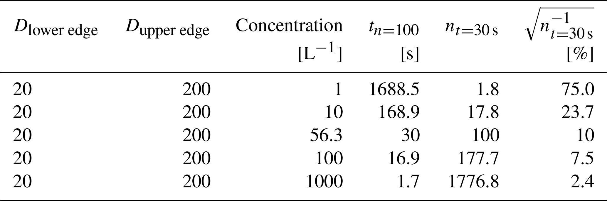
Table 2 Averaging time that is needed until n = 100 particles are sampled as well as the total number of particles sampled during an averaging time of 30 s, calculated for the size bin of 20–200 µm and exemplary particle concentrations.

4.4 Discussion: particle size distribution and statistical significance

The sampled cloud volume V_s per unit time t calculates as $V_{\mathrm{s}}=A_{\text{sens}}\cdot v\cdot t$, where v is the relative air speed and A_sens is the probe's sensitive area. A_sens is dependent on particle phase and diameter, as discussed in Sect. 4.2. Assuming a relative air speed of $v=\mathrm{150}\text{m}{\text{s}}^{-\mathrm{1}}$, the resulting sample volume amounts to about V_s = 0.08 (0.026, 0.12) L s⁻¹ for ice particles with diameter D = 200 (50, 500) µm, respectively. This is somewhat larger compared to other single-particle cloud instruments (e.g., the CPI, V_s=0.009 L s⁻¹; Lawson et al., 2001), comparable to, e.g., the SID3 (V_s=0.071 L s⁻¹, Vochezer et al., 2016) but is significantly smaller compared to the optical array probes like the 2D-C ($V_{\mathrm{s}}\simeq \mathrm{0.1}-\mathrm{10}$ L s⁻¹, Wu and McFarquhar, 2016). This has consequences for the averaging time needed in order to achieve statistically significant information on total particle concentrations.

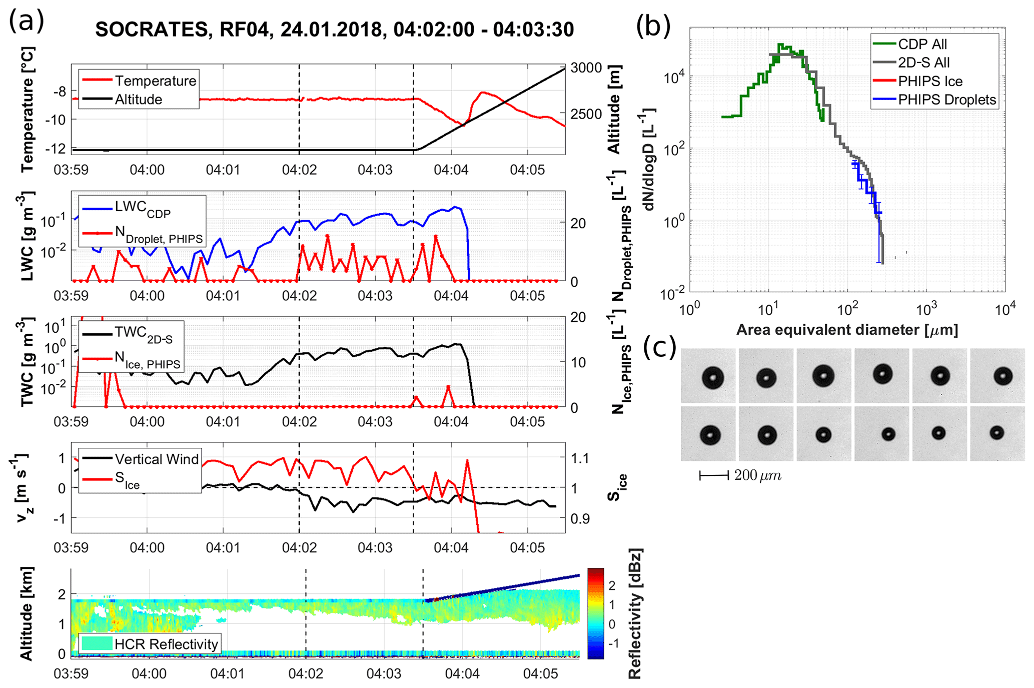
Figure 13 Example of PHIPS data acquired in a low-level supercooled liquid cloud over the Southern Ocean during the SOCRATES campaign (research flight RF04). (a) Overview of meteorological parameters, CDP, 2D-S and PHIPS number concentrations (based on the ASF data) as well as HCR radar data. (b) The comparison of the PSDs measured by CDP, 2D-S and PHIPS including statistical uncertainty bars $\sqrt{n^{-\mathrm{1}}}$ as discussed in Sect. 4.4. (c) Representative stereo micrographs of particles during that segment measured by PHIPS.

We investigated the statistical uncertainty in example situations for the total number concentration for the size range from 20 to 200 µm. This size range was chosen, since at sizes below 200 µm the phase information from PHIPS is of interest as phase detection based on traditional imaging methods can be challenging for small particle sizes. In order to reach statistical uncertainty $\propto n^{-\mathrm{0.5}}$ of less than 10 %, the number of particles per size bin needs to be larger than n>100. Table 2 shows the calculated averaging time in seconds that is needed until n = 100 particles are sampled per bin (t_n=100) and the estimated number of particles that would be sampled during 30 s of sampling (n_t=30 s), as well as the corresponding statistical uncertainty n^−0.5 for a sampling period of 30 s ($\sqrt{n_{t=\mathrm{30}\mathrm{s}}^{-\mathrm{1}}}$) for the chosen size range. All particles were assumed to be ice.

It can be seen that the ice crystal concentrations need to be larger than 56.3 L⁻¹ in order to achieve a statistical uncertainty below 10 % within 30 s. For ice crystal concentrations of 1 (10) L⁻¹ an averaging time of 28 (2.8) min would be needed, which at least in the case of low (< 10 L⁻¹) ice crystal concentrations would likely exceed the sampling duration. For optical array probes assuming a sampling volume of V_s=1.5 L s⁻¹ the corresponding sampling times would be 66.7 s and 6.7 s for concentrations of 1 and 10 L⁻¹. This shows that in order to get statistically significant size distributions, it is important to properly consider adequate averaging time and/or bin size, especially in segments with low particle concentration.

5 Case studies

In this section, the above-presented methods are applied for three representative case studies from the SOCRATES campaign in altitudes below 2000 m, one purely liquid cloud and two mixed-phase clouds. The results are then compared to the measurements of other instruments from the same flights.

5.1 Case study 1 – purely liquid cloud

Figure 13a shows meteorological and microphysical data collected during SOCRATES research flight RF04 on 24 January 2018. Taking off in Hobart, Australia, the aircraft flew southwest sampling in different types of clouds ranging from deep precipitating clouds to layer clouds in various different altitudes. The probing pattern was alternating between above-cloud sampling (for aerosol measurements) and in-cloud sampling (to investigate the microphysical properties of the cloud's hydrometeors).

A low-level supercooled liquid cloud was probed at an altitude of approximately 2100 m at a temperature of about −8.5 ^∘C at around 55^∘ S, 141^∘ E. The vertical wind velocity was at a constant value of −0.5 m s⁻¹, indicating a weak downdraft. The relative humidity with respect to ice averaged about 105 %. The liquid water content (LWC) measured with the CDP averaged around 0.1 g L⁻¹, and the total water content (TWC) measured with the 2D-S was around 0.5 g L⁻¹. The lower panel shows the radar reflectivity measured by the HIAPER (High-performance Instrumented Airborne Platform for Environmental Research) cloud radar (HCR, UCAR/NCAR-EOL, 2018), which shows a single non-precipitating cloud layer from 04:02 UTC onwards. The HCR beam was in nadir pointing mode for all three presented case studies.

The trigger threshold of PHIPS was set in a way that the instrument started to trigger on droplets with diameters larger than 50 µm. This remained unchanged over the whole campaign. The stereo micrographs from this flight segment (Fig. 13c) show the presence of large drizzle droplets with diameters from 100 to 200 µm. No indication of the presence of ice crystals was seen in the PHIPS images.

Figure 13b shows PSDs measured with the CDP (UCAR/NCAR-EOL, 2019), 2D-S (Wu and McFarquhar, 2019) and PHIPS. The PSD has a maximum at around 15 µm, and the maximum particle sizes are found at 300 µm. All the PSDs agree well with each other. Information on the phase on the largest particles can be acquired from the PHIPS ASF measurements. The phase discrimination algorithm classified every particle in the presented segment as a droplet, which is in agreement with the stereo micrographs. This shows that this cloud, despite the low temperature and the particle sizes up to 300 µm, consists purely of supercooled liquid droplets.

5.2 Case study 2 – heterogeneous mixed-phase cloud

Low-level mixed-phase clouds were investigated during SOCRATES research flight RF07 on 31 January 2018. During this flight, the aircraft sampled clouds southeast from Hobart, including an overpass over Macquarie Island. The aircraft flew at cruising altitude towards the most southward point, where it descended down to a lower altitude, probing multiple thin and persistent supercooled and mixed-phased clouds on its way back to Hobart.

Figure 14a shows a cloud segment at around −58^∘ N, 162^∘ E, shortly after the turnaround at the most southward point. The cloud was probed at an altitude of 1800 m at a temperature of about −10 ^∘C. The vertical wind velocity was slightly below zero, and the relative humidity with respect to ice averaged about 107 %. The maximum of the CDP LWC was 0.5 g L⁻¹, and the maximum of the 2D-S TWC was 2 g L⁻¹.

Figure 14 Same as in Fig. 13 but for a low-level droplet-dominated mixed-phase cloud during a transit leg of SOCRATES research flight RF07. All supercooled droplets (c) were sampled between 04:16:40 and 04:19:30, whereas the ice particles (d) were sampled between 04:19:30 and 04:21:00.

Figure 14b shows the PSDs between 04:16:40 and 04:21:00 UTC. The PSD has a maximum at 15 µm, and the maximum particle sizes are found at 700 µm. All the probes agree well. Based on the PHIPS phase information, the whole segment can be divided into two sub-segments. Until 04:19:30 PHIPS detects only supercooled liquid droplets; after that it detects only ice particles. This is backed up by PHIPS' representative stereo micrographs from the two sub-segments. In the first sub-segment, Fig. 14c shows supercooled drizzle droplets with diameters from 50 to 200 µm similar to the purely liquid case. During the second sub-segment Fig. 14d shows irregular and columnar ice crystals with sizes from 100 to 500 µm, some of which appear to be rimed or faceted. This coincides with the high-reflectivity area measured by the HCR (lower panel in Fig. 14a) and the decrease in LWC measured by the CDP. No ice particles were present on stereo micrographs taken during the first sub-segment, and no droplets were present during the second, respectively.

5.3 Case study 3 – ice-dominated mixed-phase cloud

Figure 15a shows a low-level mixed-phase cloud of SOCRATES research flight RF08 on 4 February 2018. Due to a low-pressure system south of Tasmania, cold air was expected advecting north from the Antarctic. During this flight, the aircraft flew straight southwards from Hobart. After turning back at the most southward point, the flight path back to Hobart was alternating between a “sawtooth” pattern (going up and down through the clouds) and a “staircase” pattern (10 min above the cloud, then 10 min inside the cloud and 10 min below, as explained previously).

Figure 15 Same as in Figs. 13 and 14 but for a low-level mixed-phase cloud of SOCRATES research flight RF08.

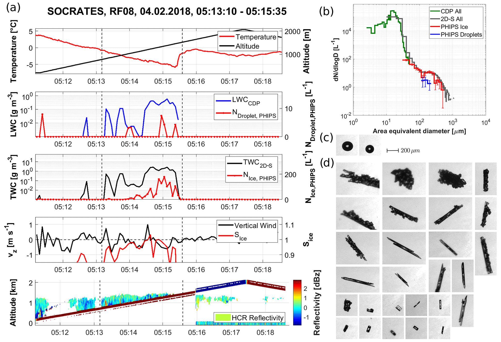
The presented case study shows one segment during the ascent of the final sawtooth leg around −51^∘ N, 147^∘ E in a thin mixed-phase cloud in the Hallett–Mossop temperature regime (Hallett and Mossop, 1974). The cloud was approximately 700 m thick, and the temperature within the cloud ranged between −5 ^∘C at the cloud base at 700 m and 0 ^∘C at the cloud top at 1400 m. The vertical wind velocity was fluctuating around zero, and the relative humidity with respect to ice was between 80 % and 100 %. The maximum of the CDP LWC was 0.5 g L⁻¹, and the 2D-S TWC was 3 g L⁻¹.

Figure 15b shows the PSDs between 05:13:10 and 05:15:35 UTC. The PSD has a maximum at 15 µm, and the maximum particle sizes are found at up to 800 µm. Again, all three probes agree well. Contrary to the previous case, the stereo micrographs in Fig. 15c and d are almost exclusively ice crystals. The sizes range from 20 to 500 µm. Observed ice crystal habits throughout the cloud were mostly needles with some hollow columns and small irregulars – all with different degrees of crystal complexity and riming. Also, a few supercooled droplets were present. The presence of supercooled droplets is also confirmed by the scattering measurements. This shows that our method is also able to detect and correctly classify single large supercooled drizzle droplets in mixed-phase clouds which are otherwise dominated by ice in that size range.

6 Conclusions

A major challenge in the observations of mixed-phase clouds remains the phase discrimination of cloud droplets and ice crystals. Especially, in the size range of D< 100 µm, reliable phase discrimination of cloud particles has proven difficult. Here, we present a new method to derive the phase of single cloud particles using their angular-light-scattering information. ASFs of single cloud particles were measured with the airborne PHIPS probe. We identified four features in the particle light-scattering function that were used for estimating the probability for the particle to be spherical or aspherical. The method was calibrated with a data set of 9738 manually classified cloud particles and tested against a data set of 12 220 manually classified particles from two different aircraft campaigns. This yields a confidence rate above 98 %. Further, we have shown that the phase discrimination algorithm is functioning independently of the experimental data set used for the calibration, so no further calibration is needed for upcoming future campaigns.

Additionally, we presented a method to derive PSDs based on single-particle scattering data for particles in a size range from 100 µm ≤ D ≤ 700 and 20 µm ≤ D ≤ 700 µm for droplets and ice particles, respectively. The newly developed data analysis algorithms were applied to three case studies that did not show the presence of large (> 1 mm) ice crystals. Comparison of the PSDs from other instruments showed a good agreement. The presented case studies show that PHIPS can provide unique and detailed insight into the phase composition of clouds, where phase discrimination based solely on particle size or aspect ratio could potentially be difficult, such as, e.g., in mixed-phase cloud conditions where large droplets and small ice crystals coexist.

With these methods available, PHIPS can provide additional information on the microphysical properties of mixed-phase clouds in situations where the data are not affected by shattering. We have also shown that phase discrimination based on single-particle angular-light-scattering behavior is a robust method, which could be implemented in future cloud research instrumentation.

Appendix A: Phase discrimination algorithm: fit parameters

To fit the normalized occurrence of the feature parameters in Fig. 6 (upper panels), a Gaussian fit function of the form

$$\begin{array}{}\text{(A1)}& n\left(x\right)=a\cdot \exp \left(-{\left({\displaystyle \frac{x-\mathit{\mu }}{\mathit{\sigma }}}\right)}^{\mathrm{2}}\right)\end{array}$$

is used. The corresponding fit parameters (with 95 % confidence intervals) for the four feature parameters for the ACLOUD data set are shown in Table A1.

Since the Gaussian distributions are of similar width σ, the corresponding discrimination probabilities (Fig. 6, lower panels), defined as

$$\begin{array}{}\text{(A2)}& P\left(f\right)={\displaystyle \frac{n_{\text{ice}}\left(f\right)}{n_{\text{ice}}\left(f\right)+n_{\text{droplet}}\left(f\right)}},\end{array}$$

can be approximated by a sigmoid function of the form

$$\begin{array}{}\text{(A3)}& P\left(x\right)={\displaystyle \frac{a-d}{\mathrm{1}+\exp (-b\cdot (x-c\left)\right)}}+d.\end{array}$$

The corresponding fit parameters are shown in Table A2.

Table A1 Fit parameters of the Gaussian fits for the distribution of the feature parameters n_i.

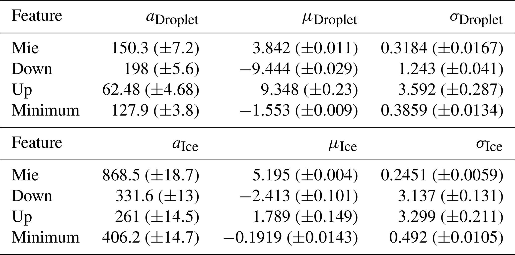
Table A2 Fit parameters of the sigmoid fit for the discrimination probabilities P_i.

Appendix B: Phase discrimination algorithm: cross-correlation of the feature parameters

In Sect. 3.3 we have argued that one feature alone is not sufficient to reliably classify all cloud particles, due to the particles that lie in the overlap between the two peaks in Fig. 6. Now the question is how dependent the four features are and whether or not a particle that cannot be confidently (or is even falsely) classified by, e.g., f₃, i.e., which lies in the overlap of the feature space, can be confidently classified by the other feature parameters or if it lies in the overlap for the other features as well.

Figure B1a shows the correlation of the classification confidence based on only one feature parameter f₃ and of the combined result for all four features for all manually classified ice particles of the ACLOUD campaign. It can be seen that lots of particles that cannot be classified with high confidence by the first feature (P(f₃)<66 %) are classified with high confidence by the other features (P_combined>66 %). The corresponding statistics are displayed in a confusion matrix in Fig. B1b. It can be seen that most of the particles (87.5 %) are correctly and confidently classified based on f₃ alone (column 4). But out of the 992 particles that are not classified confidently and correctly based on f₃ (i.e., sum of columns 2 and 3) most (805) are confidently classified based on the combination of all four features. This shows that the usage of multiple features significantly improves the discrimination accuracy. Hence, by combining all four different features, a high combined classification confidence can be achieved as shown in Fig. S6a in the Supplement.

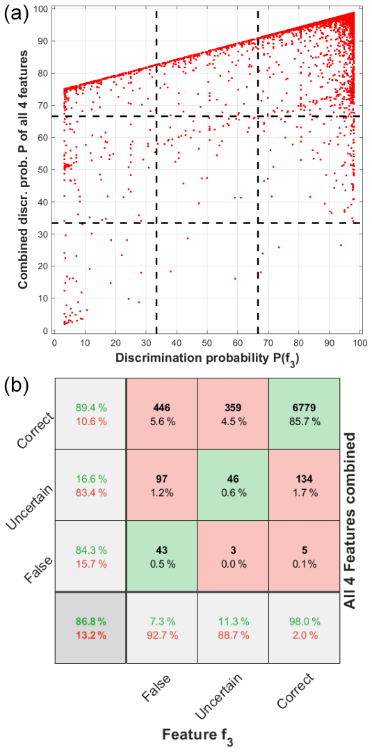
Figure B1 (a) Correlation of the discrimination (classification) probability of feature parameter f₃ alone and the combination of all four features. The dashed lines mark the confidence limits. P(f)>66 % corresponds to particles that are classified correctly with high confidence; $\mathrm{33}<P\left(f\right)\le \mathrm{66}\mathit{\%}$ means the classification is uncertain; and particles with P(f)≤33 % are classified falsely as droplets with high confidence. Panel (b) shows the corresponding statistics of the plot in a confusion matrix. The squares correspond to the dashed lines in (a).