Retrieval of atmospheric CO₂ vertical profiles from ground-based near-infrared spectra

We evaluate vertical profile retrievals of CO₂ from 0.02 cm⁻¹ resolution ground-based near-infrared solar absorption spectra with the GFIT2 algorithm, using improved spectroscopic line lists and line shapes. With these improvements, CO₂ profiles were obtained from sequential retrievals in five spectral windows with different vertical sensitivities using synthetic and real spectra. A sensitivity study using synthetic spectra shows that the leading source of uncertainty in the retrieved CO₂ profiles is the error in the a priori temperature profile, even with 3-hourly reanalysis a priori profiles. A 2 ^∘C error in the temperature profile in the lower troposphere between 0.6 and 0.85 atm causes deviations in the retrieved CO₂ profiles that are larger than the typical vertical variations of CO₂. To distinguish the effect of errors in the a priori meteorology and trace gas concentration profiles from those in the instrument alignment and spectroscopic parameters, we retrieve CO₂ profiles from atmospheric spectra while using an a priori profile built from coincident AirCore, radiosonde, and surface in situ measurements at the Lamont, Oklahoma (USA), Total Carbon Column Observing Network station. In those cases, the deviations in retrieved CO₂ profiles are also larger than typical vertical variations of CO₂, suggesting that remaining errors in the forward model limit the accuracy of the retrieved profiles. Implementing a temperature retrieval or correction and quantifying and modeling an imperfect instrument alignment are critical to improve CO₂ profile retrievals. Without significant advances in modeling imperfect instrument alignment, and improvements in the accuracy of the temperature profile, the CO₂ profile retrieval with GFIT2 presents no clear advantage over scaling retrievals for the purpose of ascertaining the total column.

1 Introduction

Carbon dioxide (CO₂) is the most abundant well-mixed greenhouse gas in the atmosphere and the main driver of the increase in global mean surface temperatures since the start of the industrial era (Ciais et al., 2013; Myhre et al., 2013). A yearly global carbon budget has been produced by the Global Carbon Project since 2012 (Friedlingstein et al., 2019; Le Quéré et al., 2013, 2014, 2015b, a, 2016, 2018b, a). It presents current knowledge of CO₂ emissions to inform policies that aim to reduce the emissions of greenhouse gases into the atmosphere. The project uses ensembles of models and inventories, as well as CO₂ surface measurements, to estimate different components of the global emissions of CO₂. It also uses CO₂ fluxes obtained from atmospheric inversions (Chevallier et al., 2005; van der Laan-Luijkx et al., 2017; Rödenbeck et al., 2003; Saeki and Patra, 2017) as a semi-independent validation tool for these estimates; most of the CO₂ measurements used in these inversions come from surface networks. Since 2014, the project makes mention of the potential of inversions using space-based measurements of total column CO₂ to provide additional constraints on sources and sinks of CO₂.

Column-averaged dry-air mole fractions of CO₂ (XCO₂), are retrieved from solar absorption spectra measured from space by the Atmospheric InfraRed Sounder (AIRS, Aumann et al., 2003), the Greenhouse gases Observing SATellite (GOSAT and GOSAT-2) (Kuze et al., 2009, 2016; Nakajima et al., 2012), the Orbiting Carbon Observatory (OCO-2 and OCO-3) (Crisp, 2008, 2015; Eldering et al., 2019), and Tansat (Liu et al., 2018). CO₂ fluxes obtained from inversions assimilating OCO-2 observations over land are now becoming as reliable as those obtained from inversions using surface air sampling networks (Chevallier et al., 2019). Measurements of XCO₂ by satellites can be made with unprecedented spatial coverage. Inversions using CO₂ total columns over land are less sensitive to transport errors than inversions using surface CO₂ (Basu et al., 2018; Rayner and O'Brien, 2001), which require accurate modeling of the planetary boundary layer height and vertical mixing, both of which are a major source of uncertainty in inversions (Parazoo et al., 2012). However, even small (< 1 ppm) spatially coherent biases in column measurements can have a large impact on inversions assimilating XCO₂ (Chevallier et al., 2007), and efforts must be made to characterize and minimize such biases (Kiel et al., 2019; O'Dell et al., 2018).

The Total Carbon Column Observing Network (TCCON) is a ground-based network of high-resolution (0.02 cm⁻¹) ground-based Fourier transform infrared (FTIR) spectrometers that record shortwave IR (SWIR) solar absorption spectra (Wunch et al., 2011b). TCCON produces retrievals of XCO₂ which are widely used to validate satellite observations and to study the carbon cycle (Wunch et al., 2011a, 2017; Keppel-Aleks et al., 2012, 2013). New versions of the TCCON retrieval algorithm (GGG) are released every few years, and each new version is designed to improve the quality of the data.

GGG2014 (Wunch et al., 2015) is the current version of the GGG software used by TCCON to transform measured interferograms into spectra, and then to retrieve trace gas mixing ratios from those spectra. Central to this process is GFIT, a non-linear least-squares spectral fitting algorithm. A forward model computes an atmospheric transmittance spectrum for a given observation geometry using a priori knowledge of atmospheric conditions and assuming a perfectly aligned instrument. An inverse method then compares the measured spectrum with the resulting calculation and adjusts the retrieved parameters to obtain the best fit. In GFIT, these parameters include volume mixing ratio scaling factors (VSFs) for the different fitted gases. GFIT performs profile scaling retrievals: for each retrieved trace gas, a single VSF scales the entire a priori concentration profile at all altitude levels simultaneously and therefore the retrieved profile shape is unchanged from the a priori profile shape. Technically, GFIT handles the scaling retrieval by weakly constraining the fitted VSF factor. The approach is equivalent to performing an optimal estimation of the VSF, assigning a value of unity to the a priori VSF and a value of 10⁶ as its expected range of variability. XCO₂ can be retrieved with a 2σ precision and accuracy of 0.8 ppm (Wunch et al., 2010). GFIT minimizes the spectral fit residuals: the difference between the measured and calculated spectra. The measurement noise is not required to be accurately known; all retrievals from TCCON CO₂ windows use an assumed signal-to-noise ratio (SNR) of ∼ 200. This assumption has only a small effect on the result because for CO₂ the absorption line depths and the spectral fitting residuals far exceed the measurement noise.

Even though TCCON XCO₂ observations are precise and accurate, they explicitly lack information about the vertical distribution of CO₂ in the atmosphere, which is of interest for the validation of satellite measurements and model simulations and could improve the ability of atmospheric inversions to resolve emissions at regional scales (Keppel-Aleks et al., 2011). The most precise and accurate sources of information on CO₂ vertical profiles are provided by air samples collected at different altitudes using weather balloons or aircraft, but these observations are sparse in space and time. Aircraft vertical profiles are used as validation tools for inversion studies (Peters et al., 2007; Stephens et al., 2007; Pickett-Heaps et al., 2011), which requires them to remain independent from the inversion systems (Chevallier et al., 2019). Obtaining reliable CO₂ profile information from ground-based direct-sun measurements could significantly augment the number of observations available for verification and assimilation in atmospheric inversions, and would allow TCCON to be used for validation of thermal infrared satellite products, e.g., from AIRS and GOSAT/2, and vertically resolved NIR GOSAT and OCO-2 experimental products. Vertical profile information derived from ground-based absorption spectra cannot be as accurate as aircraft-based vertical profiles, and would also be spatially sparse, but would provide a higher temporal sampling.

CO₂ profile retrievals from ground-based SWIR spectra have been calculated using the band centered at 1.6 µm with a Voigt line shape (Kuai et al., 2012), and in the band centered at 2.06 µm with the PROFFIT optimal estimation software package (Hase et al., 2004) fitted with a Voigt line shape with line mixing (Dohe, 2013). In our approach, we use the GFIT2 software package initially described by Connor et al. (2016), which is a profile retrieval algorithm based on the GGG software suite, but modified such that it allows the profile shape to vary during the retrieval process. Instead of retrieving a single VSF value that scales the whole a priori profile, a VSF value is retrieved for each atmospheric level. The algorithm thus has much more freedom to fit the observed spectra but is also more sensitive to uncertainties in the forward model calculations such as errors in the atmospheric temperature profile, spectroscopic errors, and instrument misalignment, for example.

Connor et al. (2016) showed that CO₂ profile retrievals in the CO₂ band centered at 1.6 µm are very sensitive to errors in spectroscopy. GFIT2 was first developed using the GGG2014 version of the GGG suite (Wunch et al., 2015), which uses a Voigt line shape to compute absorption coefficients. In this study, we use the GGG2020 version, which will be released in early 2021. This version of the code implements quadratic speed-dependent Voigt line shapes with line mixing (qSDV+LM) for CO₂ (Mendonca et al., 2016) and CH₄ (Mendonca et al., 2017) bands, and qSDV line shapes for O₂ in the band centered at 1.27 µm (Mendonca et al., 2019). The line mixing coefficients are derived with the first-order Rosenkranz approximation (Rosenkranz, 1975). This leads to significantly better spectral fits, especially in the strong CO₂ band centered at 2.06 µm, and smaller variations of gas amount with air mass. Other improvements to the forward model include (1) updates to the spectroscopic line list (Toon, 2015) (2) a solar-gas stretch fitted to account for Doppler-driven differences between solar and telluric wavenumber scales (in GGG2014 only the stretch in the telluric wavenumber scale was fitted), and (3) improved a priori profiles as described in Sect. 2.2.

This study assesses the quality of CO₂ profile retrievals with GFIT2 implemented in GGG2020. Section 2 describes the retrieval algorithm and our methodology. Section 3 presents a sensitivity study using synthetic spectra, followed by retrievals using real measured spectra. Finally, Sect. 4 presents a summary of the results and conclusions.

2 Methods

In this study, GFIT2 is used to retrieve CO₂ profiles from the two original TCCON retrieval windows and three new windows that possess a large range of opacities, and therefore vertical sensitivities. These windows are presented in Table 1 and Fig. 1. The TCCON1 window (centered at 6220 cm⁻¹) and TCCON2 window (centered at 6339.5 cm⁻¹) are used to derive XCO₂ in the public TCCON data products, because the spectral absorption line opacities are close to 1 and are therefore equally sensitive at most altitudes. The CO₂ line intensities in the weak windows are 10 times smaller than in the standard TCCON windows, providing more sensitivity to CO₂ variations aloft. The CO₂ lines in the “Strong” window are 15 times stronger than those in the standard TCCON windows, providing more sensitivity to CO₂ variations near the surface. All windows have an average lower-state energy (E^′′) of roughly 240 cm⁻¹, rendering the retrieved total column of CO₂ highly independent of the assumed temperature (< 0.1 % K⁻¹). The derivation of XCO₂ as calculated in GGG is described in Appendix A. XCO₂ is the ratio of the CO₂ column to the column of dry air, and the column of dry air is expressed as the retrieved O₂ column (from the window centered at 7885 cm⁻¹; see Table 1) divided by 0.2095 (Wunch et al., 2011b). OCO-2/3 and GOSAT/2 use two windows comparable to the TCCON1 and Strong windows to retrieve CO₂ and use the O₂ A-band (centered near 13158 cm⁻¹).

Table 1 CO₂ spectral windows used with GFIT2. Interfering absorbers labeled “solar” are due to absorption by heavy metal ions (e.g., Fe, Si, Ca, Ni) in the solar photosphere. Also shown are the strength-weighted averages of the lower-state energy (E^′′) and of the line strengths (S) over all the CO₂ lines in each window. The column of O₂, retrieved with scaling retrievals from the O₂ window, is used to compute XCO₂.

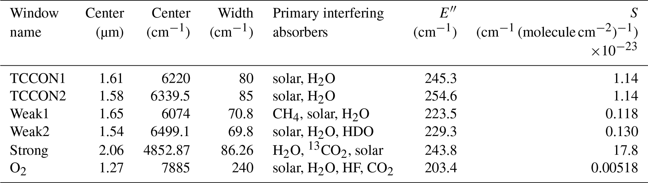
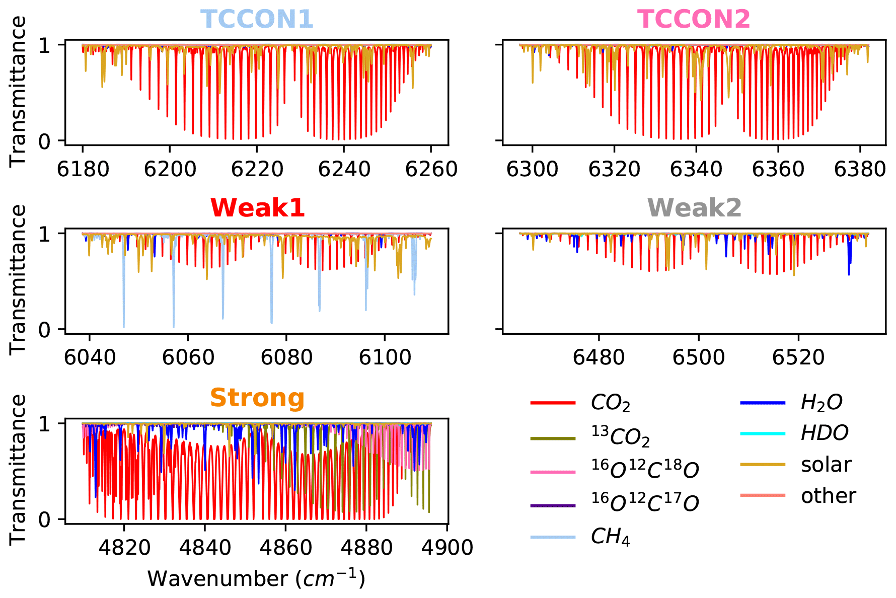
Figure 1 Contributions of different absorbing gases to the calculated transmittance spectrum on a dry winter day at a solar zenith angle of 60.6^∘ for each of the spectral windows used to retrieve CO₂.

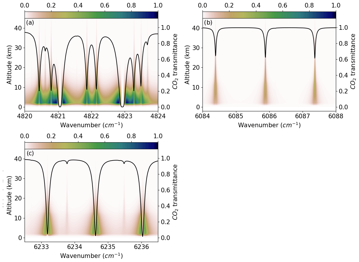
Figure 2 CO₂ absorption lines (black line) overlaid on heat maps of the CO₂ Jacobian for lines of (a) the Strong window, (b) the Weak1 window, and (c) the TCCON1 window. The color bar represents the normalized Jacobian where 1 corresponds to the maximum amongst all the CO₂ Jacobians from the five CO₂ windows. Lines of the Weak2 and TCCON2 windows are not shown as they look like the Weak1 and TCCON1 windows, respectively.

A qualitative representation of the vertical sensitivity due to the range of different line opacities is presented in Fig. 2, which shows the normalized CO₂ Jacobian for typical absorption lines in the Strong window (centered at 4852.87 cm⁻¹), the “Weak1” window (centered at 6074 cm⁻¹), and the TCCON1 window (centered at 6220 cm⁻¹). The strong saturated lines of the Strong window are more sensitive to levels below 5 km than in the TCCON1 window, but the Strong window also contains lines of intermediate absorption strength that provide more uniform sensitivity up to ∼ 10 km, and that extend the window's sensitivity to up to 30–40 km. The saturated lines in the Strong window correspond to the 20013–00001 band, while the lines of intermediate strength around 4820 cm⁻¹ come from the R branch of the 21113–01101 band. The TCCON1 window has more uniform sensitivity up to ∼ 10–15 km and contains weak lines which contain information on CO₂ above 15 km. The Weak1 window is less sensitive below 10 km and has more uniform sensitivity between 10–20 km. Figure 2 also shows little to no sensitivity to levels above ∼ 30 km in all windows.

2.1 Retrieval algorithm

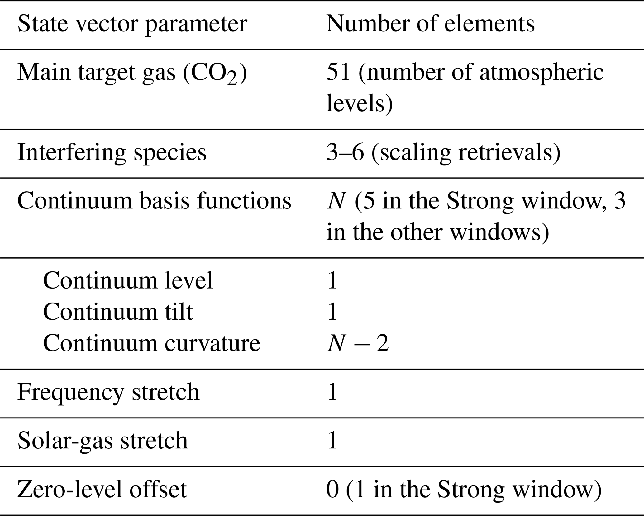
The GFIT2 retrieval algorithm is described in detail in Appendix B and follows the formulation of Rodgers (2000). Currently, GGG has no option to simultaneously retrieve information about a gas from spectral windows that are not contiguous in wavenumber. Therefore, we retrieve trace gas information from each window separately. We see no advantage to fitting non-contiguous windows simultaneously, rather than separately, and then combining the results. In TCCON post-processing, the total columns retrieved from different retrieval windows (CO₂ from the TCCON1 and TCCON2 windows, for example) are averaged after removing window-dependent multiplicative biases, using retrieval errors as weights. Table 2 summarizes the components of the state vector used in GFIT2. A total of 51 VSFs are retrieved (one for each atmospheric level) for the primary target gas, while only 1 VSF is retrieved for each of the interfering species profiles (non-¹²C¹⁶O₂ species included in Fig. 1, except for “solar” and “other”; other CO₂ isotopologues are only retrieved as interfering species in the Strong window). Aside from the retrieved gases, other fitted parameters are part of the state vector. Orthogonal continuum basis functions are used to fit the shape of a spectrum's continuum, with different orders of curvature. An overall frequency stretch is retrieved for all lines, and a second “solar-gas” stretch is retrieved to correct for differences between the solar and telluric wavenumber scales. A zero-level offset is also retrieved in the Strong window that makes use of saturated lines.

Table 2 Components of the state vector in GFIT2 profile retrievals. These are all the retrieved parameters.

In principle, a CO₂ profile retrieval should have little sensitivity to errors in the a priori CO₂ profile (differences from the true profile) since it can adjust for differences between measured and calculated spectra caused by erroneous prior profile shapes (Connor et al., 2016). However, the retrieval may also conflate errors due to other sources, such as incorrect spectroscopic parameters, incorrect modeling of the instrument line shape, or errors in the a priori meteorology and profiles of interfering species, with these errors in the a priori CO₂ profile.

2.2 Datasets

CO₂ and CH₄ a priori profiles were built by combining the balloon-borne AirCore (Karion et al., 2010) profiles with surface in situ measurements, adding the GGG2020 a priori profile above the maximum altitude sampled by AirCore. These composite profiles will be referred to as “truth”. The CH₄ profile is included because CH₄ is an interfering gas in the Weak1 window. AirCore is a sampling system that consists of a long, coiled stainless-steel tube initially filled with a dry calibrated gas. As a balloon carries it up, the fill gas evacuates. When the AirCore descends from the stratosphere, ambient air enters the tube through the open end. Upon landing, the AirCore is quickly retrieved for subsequent laboratory analysis, wherein the sample is pushed through a continuous gas analyzer. The first gases to come out were the last to enter, and vice versa, allowing the preserved atmospheric trace gas concentration profiles to be derived. This method has precision similar to, or better than, discrete gas flask samples, with a repeatability of 0.07 ppm for CO₂ concentrations (Karion et al., 2010). The balloons reach ∼ 30 km altitude, with profiles retrieved to ∼ 25km, and therefore sample 98 % of the mass of the atmosphere. In Sect. 3.2, AirCore profiles from the v20181101 dataset were used as “truth” to assess the quality of GFIT2 profile retrievals. We used all AirCore profiles measured over the Lamont TCCON station that had coincident ground-based measurements within ±1 h of the AirCore landing and within ±1.5 h of the closest a priori time. All figures showing profiles use the average of profiles retrieved from the coincident spectra. The launch dates of the eight AirCore profiles used are presented in Table 3. An iMet-1 radiosonde carried by the same balloon as the AirCore provides in situ temperature and relative humidity profiles.

Table 3 AirCore launch dates and number of coincident spectra within ±1 h of the AirCore last sampling time and within ±1.5 h of the closest a priori time. The range of solar zenith angles covered by the coincident spectra is also shown.

Instead of the diagonal prior covariance used in Sect. 3.1, a more realistic CO₂ prior covariance matrix was built for retrievals with real spectra in Sect. 3.2. The difference between GGG2020 a priori CO₂ profiles and aircraft profiles (Biraud et al., 2013) over Lamont from NOAA's ObsPack (Sweeney et al., 2017) between 500 and 5000 m were computed for 382 aircraft profiles and for each month between 2008 and 2016. The mean difference profile plus 1 standard deviation of the month with the largest differences, August, was used to build the diagonal of the a priori covariance matrix. The a priori CO₂ uncertainty can be expressed as

$$\begin{array}{}\text{(1)}& {\mathit{\sigma }}_i=\mathrm{3.99}{e}^{-\mathrm{0.92}{\mathbf{x}}_i}+\mathrm{0.98},\end{array}$$

where x is the altitude of the ith atmospheric level in kilometers. The a priori covariance is expressed as

$$\begin{array}{}\text{(2)}& {\displaystyle }{\mathbf{z}}_{i,j}={\mathbf{x}}_i,\text{(3)}& {\displaystyle }{\left(\mathbf{\Delta }\mathbf{z}\right)}_{i,j}=\left|{\mathbf{z}}_{i,j}-{\mathbf{z}}_{i,j}^T\right|,\text{(4)}& {\displaystyle }{\left({\mathbf{S}}_{\mathrm{a}}\right)}_{i,j}={\left({\mathit{\sigma }}^T\mathit{\sigma }\right)}_{i,j}\times e^{-\frac{{\left(\mathbf{\Delta }\mathbf{z}\right)}_{i,j}}{h}},\end{array}$$

where z is a matrix with each row containing the altitude profile, Δz is the matrix of absolute altitude differences between each level, S_a is the a priori covariance matrix, and h is the length scale of interlayer correlations. The length scale was set to 2 km based on the width of the rows of correlation matrices built from the ensemble of aircraft vertical profiles.

The vertical grid used in the retrievals presented in this study has 51 levels between 0 and 70 km, and the spacing between levels increases with altitude (see Appendix A). Figure 3 shows the a priori uncertainty as a function of pressure for each of the eight a priori states used to process the Lamont spectra presented in Table 3.

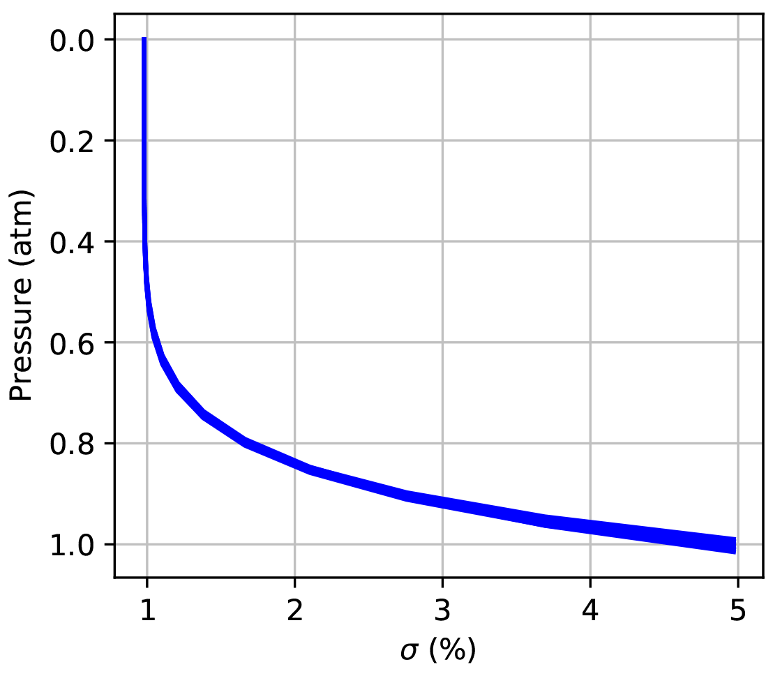
Figure 3 A priori uncertainty profiles for each of the 10 dates presented in Table 3. These are defined by Eq. (1). Since σ is defined on an altitude grid, it varies slightly with pressure.

Since the AirCore profiles do not extend down to the surface or above about 25 km, other sources are used to complete the “true” CO₂ profile. The TCCON spectrometer used in this study is located at the US Department of Energy Atmospheric Radiation Measurement program (ARM) central facility in Lamont, Oklahoma. The facility hosts a suite of instruments for remote and in situ measurements of the atmosphere. When available within 5 h of the last AirCore sampling time, surface CO₂ and CH₄ measurements from precision gas systems were used (Biraud and Moyes, 2001). When they were not available, measurements from discrete flask samples were used (on 23 July 2013, 27 February 2014, and 17 September 2014) (Biraud et al., 2002). Surface pressure, temperature, and relative humidity were obtained from in situ measurements at the Lamont central facility.

GGG2020 uses 3-hourly a priori profiles of the atmospheric state. For each spectrum in the retrievals, GGG uses the nearest a priori profile in time. The a priori meteorology and H₂O profiles are obtained from analyses of the Global Modeling and Assimilation Office (GMAO) Goddard Earth Observing System Version 5 Forward Processing for Instrument Teams (GEOS5-FPIT) (Lucchesi, 2015). The CO₂ a priori profiles are constructed from the deseasonalized NOAA Mauna Loa and Samoa flask data (Dlugokencky et al., 2019) by determining the transport lag between the measurement site and each level of the a priori profile (Laughner et al., 2021a, b). In the troposphere, this is done with an age-of-air formula and an effective latitude that accounts for synoptic motion of air. In the stratosphere, this is obtained from an age climatology derived from a chemical Lagrangian model (McKenna, 2002) of the stratosphere using equivalent latitude to account for air motion. The stratospheric priors also account for turbulent mixing with age spectra (Andrews et al., 2001). A seasonal cycle parametrization is then applied, and the resulting CO₂ profiles are corrected to match the CO₂ latitudinal gradients observed by the High-Performance Instrumented Airborne Platform for Environmental Research (HIAPER) Pole-to-Pole Observations (HIPPO) (Wofsy, 2011) and by the Atmospheric Tomography (ATom) mission (Wofsy et al., 2018).

2.3 Information content and degrees of freedom

The information content in the profile retrieval can be quantified using the averaging kernel matrix A (Rodgers, 2000). The information content H is defined as

$$\begin{array}{}\text{(5)}& H=-{\displaystyle \frac{\mathrm{1}}{\mathrm{2}}}\ln \left(\left|\mathbf{I}-\mathbf{A}\right|\right),\end{array}$$

where “ln” is the natural logarithm and |I−A| is the determinant of the difference between the identity matrix and the averaging kernel matrix. The degrees of freedom for signal (DOFs) can be expressed as

$$\begin{array}{}\text{(6)}& \mathrm{DOFs}=\mathrm{tr}\left(\mathbf{A}\right).\end{array}$$

The DOFs can be divided into the CO₂ profile DOFs and the DOFs corresponding to the rest of the state vector elements. The profile DOFs can be interpreted as the number of independent pieces of information that improve the retrieved CO₂ profiles compared to the a priori profile. The DOFs are shown in Figs. 4–7 and 9–10.

3 Results

In Sect. 3.1, we investigate the sensitivity of the profile retrievals to different sources of error using synthetic spectra produced by running the GGG forward model with a given set of atmospheric conditions. The resulting spectra were then used as input to the profile retrieval algorithm using the same set of atmospheric conditions, except for a perturbation in either the CO₂, temperature, or H₂O profiles, or in the spectroscopic parameters of CO₂ lines (air- and self-broadened half-width coefficients and their temperature dependence). In these retrievals, the SNR of the spectrum to be fitted is set to 1000 and the CO₂ a priori covariance matrix is diagonal with 5 % (∼ 20 ppm) uncertainty at all levels. No noise is added to the calculated spectra, but the assumed 1000 : 1 SNR is used to build the measurement covariance matrix and affects the relative weight of the measurement and the a priori profile. The weak prior constraint and high SNR serve to highlight the sources of variability in the retrieved profiles.

In Sect. 3.2, CO₂ profile retrievals are tested with atmospheric solar absorption spectra measured at the TCCON site in Lamont, Oklahoma (USA). If the forward model were perfect and the a priori state equal to the true state of the atmosphere, the retrieved scale factor at each level would be equal to 1. However, errors in the forward model (including spectroscopy, a priori meteorological information, radiative transfer, and instrument line shape) cause the retrieved scale factors to deviate from 1. To isolate the effect of instrument misalignment and errors in spectroscopic parameters from errors in a priori meteorology, we build a priori profiles of H₂O, temperature, CO₂, and CH₄ using in situ measurements. In Sect. 3.2 we also use an a priori covariance matrix with off-diagonal elements based on comparisons between the a priori profile and aircraft profiles, as described in Sect. 2.2.

3.1 Synthetic spectra

In this section, we attempt to identify the main sources of error in the retrieved CO₂ profiles. To do this we use synthetic spectra that are calculated with GFIT's forward model for a given set of inputs (atmospheric conditions and spectroscopic parameters). These “perfect” synthetic spectra are then used as measurements to be fitted in retrievals with one perturbed input. Thus, when the perturbed input is not the a priori CO₂ profile itself, the a priori CO₂ profile is the “truth”. In Sect. 3.1.1, we look at the ability of the retrieval algorithm to retrieve CO₂ when it is the only unknown.

Over the course of a day, the water vapor profile can vary by 40 % and the temperature profile can vary by more than 10 ^∘C in the lowest troposphere, and therefore 3-hourly a priori meteorological information could differ from the true atmospheric state by several degrees Celsius for temperature and by 10 % for water vapor. In Sect. 3.1.2, we perturb the a priori H₂O profile, the main interfering absorber. In Sect. 3.1.3, we perturb the temperature profile, as the intensity and width of all absorption lines depend on temperature. Finally, in Sect. 3.1.3 we perturb spectroscopic line parameters themselves to within their uncertainties.

The total retrieval random error for the retrievals presented in this section is ∼ 4.5 % (∼ 18 ppm), and the contribution of random noise is ∼ 0.8 % (∼ 3 ppm); see Appendix D for definitions of total and measurement noise errors. When the deviations from the truth are larger than the a priori uncertainty (∼ 20 ppm), it means the perturbation applied has a severe effect on the retrieval. Of course this can be mitigated by using a stronger a priori constraint or a measurement covariance matrix that reflects expected systematic errors, and not just random noise, but always at the cost of reduced sensitivity to CO₂ too. The goal here is to estimate the relative effect of different kinds of expected systematic errors on retrieved profile shapes. Stronger constraints can only reduce the amplitude of the deviations from the truth, but the same structures would remain. When the perturbation to a parameter other than CO₂ results in deviations from the truth much larger than those presented in Sect. 3.1.1, it means that errors in that parameter will dominate the variability in the retrieved CO₂ profiles regardless of the retrieval constraints.

3.1.1 Perturbed CO₂ profile

With a perturbed CO₂ prior profile, the algorithm can retrieve the true profile shape very well in all windows, even with an a priori profile vastly different from the truth as shown in Fig. 4. In Fig. 4a, when using the same prior that generated the synthetic spectrum, the retrieved profiles do not align exactly with the prior profile. This is due to small imperfections in the synthetic spectra, but these result in differences of less than 1 ppm at any altitude. In Fig. 4c the standard GGG2020 a priori profile is used as the a priori profile, while the “true” CO₂ profile used to generate the synthetic spectrum was built from a composite “true” profile as described in Sect. 2.2. In each window the retrieved profile is within 2 ppm of the truth. In Fig. 4e a constant CO₂ profile with 380 ppm at all levels is used as the a priori profile. Again, the retrieved profiles are within 2 ppm of the truth except at the bottom and top of the profile where most of the information comes from the a priori profile. This self-consistency test shows that the GFIT2 algorithm works as expected and can accurately retrieve CO₂ when the a priori CO₂ profile is the only source of uncertainty.

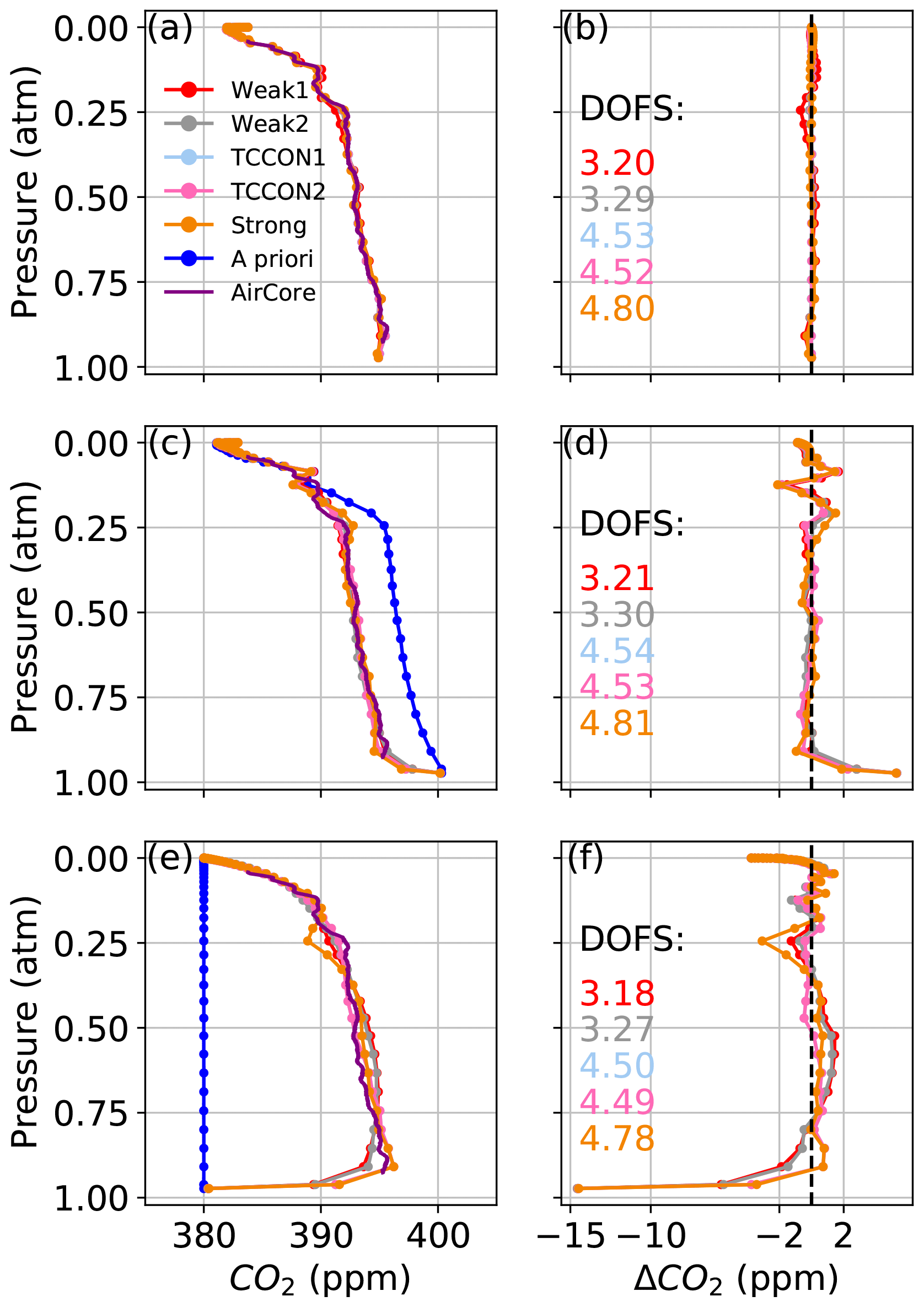
Figure 4 The left-hand panels show CO₂ profiles retrieved using synthetic spectra. In (a), we use the AirCore profile, which was used to generate the synthetic spectra, as the a priori profile. In (c), we use the GGG2020 a priori CO₂ profile as the a priori profile. In (e), we use a constant CO₂ a priori profile. Panels (b), (d), and (f) show the difference between the retrieved profiles and AirCore, corresponding to (a), (c), and (e) respectively.

3.1.2 Perturbed H₂O profile

Figure 5 shows the effect of a +10 % perturbation to the H₂O vapor profile below 5 km for a dry winter day and a wet summer day. It leads to 2 ppm deviations from the CO₂ a priori profile in the Strong window under dry conditions and up to 15 ppm under wet conditions. In both cases, the deviations from the truth in the CO₂ profiles retrieved from the other windows were within 2 ppm.

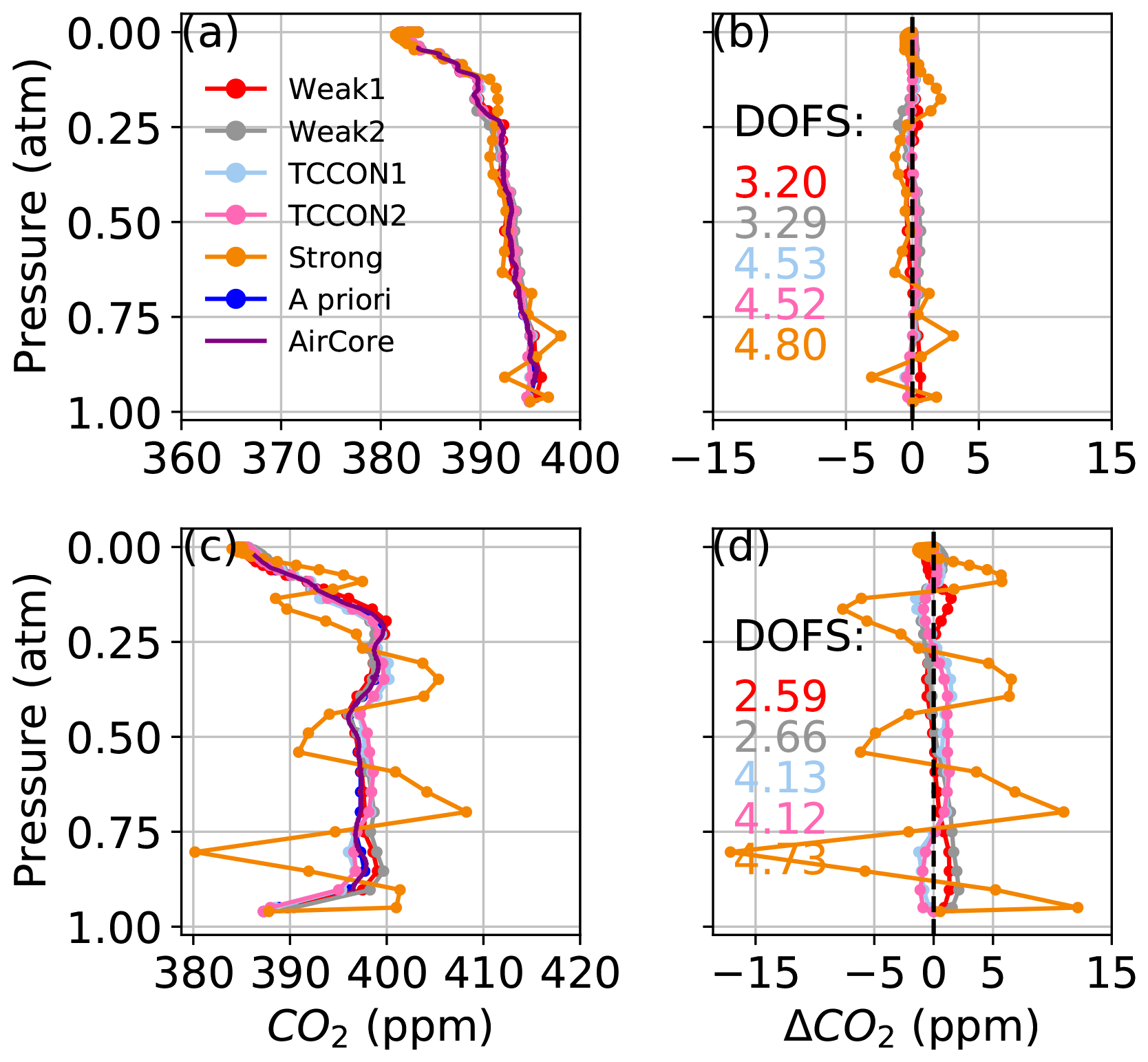
Figure 5 The left-hand panels show CO₂ profiles retrieved using synthetic spectra. 10 % is added to the H₂O profile below 5 km for (a) dry conditions on 14 January 2012 and for (c) wet conditions on 23 July 2013. Panels (b) and (d) show the difference between the retrieved profiles and AirCore, corresponding to (a) and (c) respectively.

3.1.3 Perturbed temperature profile

A +5 ^∘C perturbation to the temperature profile below 5 km (0.5 atm < P < 1.0 atm), as in Fig. 6a, leads to deviations from the truth in the retrieved CO₂ profiles of up to 50 ppm in the Weak and TCCON windows, and up to 100 ppm in the Strong window. In that case the fit residuals can exceed 1 % in the Strong window and 0.5 % in the TCCON windows. For the retrievals used to obtain the profiles in Fig. 6a the SNR was set to 100 in the Strong window, 200 in the TCCON windows, and 1000 in the Weak windows. In Fig. 6c and e the SNR is set to 1000 in all windows. In Fig. 6c, a +2 ^∘C perturbation is applied between 8 and 13 km (0.2 atm < P < 0.35 atm). The amplitude of deviations in the TCCON windows and in the Strong window is close to 50 ppm at ∼ 0.9 atm and 100 ppm at ∼ 0.2 atm. In the two Weak windows, the deviation amplitude is ∼ 10 ppm at ∼ 0.9 atm and ∼ 20 ppm at 0.2 atm. In Fig. 6e, a +2 ^∘C perturbation is applied above 15 km. In the Strong window, the resulting deviation at pressures > 0.6 atm has the smallest amplitude amongst the five windows, within 4 ppm, and the deviation at ∼ 0.2 atm is ∼ 20 ppm. In the TCCON windows, the deviation at pressures > 0.6 atm is reduced to ∼ 10 ppm while the deviation at pressures > 0.6 atm is comparable to that in Fig. 6b. In the two Weak windows, the deviation at ∼ 0.9 atm is unchanged when to compared to Fig. 6b and the deviation at ∼ 0.2 atm is reduced from ∼ 15 to ∼ 10 ppm.

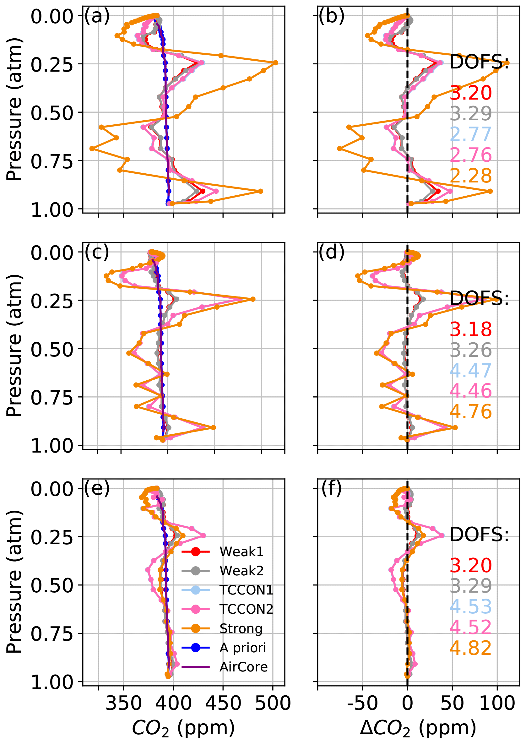
Figure 6 The left-hand panels show CO₂ profiles retrieved using synthetic spectra for (a) +5 ^∘C added to the a priori temperature profile below 5 km, (c) +2 ^∘C between 8 and 13 km, and (e) +2 ^∘C above 15 km. Panels (b), (d), and (f) show the difference between the retrieved profiles and AirCore profile, corresponding to (a), (c), and (e) respectively. Note the difference in the horizontal axis range between the panels. Here 5 km corresponds to ∼ 0.55 atm, 8–13 km to ∼ 0.36–0.17 atm and 15 km to ∼ 0.125 atm.

From the results in Sect. 3.1.1, 3.1.2, and 3.1.3, we observe that CO₂ profile retrievals do not need accurate prior knowledge of the CO₂ profile but require accurate knowledge of the prior temperature and water vapor profiles. Moreover, these results suggest that errors in the temperature profile are the main source of deviations from the truth in retrieved CO₂ profiles. Retrievals using the two Weak windows are the least affected by biases in the prior temperature and water vapor profiles. The need for accurate a priori water vapor profile could be alleviated by retrieving H₂O profiles simultaneously with CO₂ profiles, but this was not tested with GFIT2, which currently can only retrieve the main target gas in a window with profile retrievals. In addition, H₂O profile retrievals would also be affected by temperature errors.

3.1.4 Perturbed line parameters

The line list used by GGG is a compilation of different versions of the HITRAN line lists (Gordon et al., 2017; Rothman et al., 2005, 2009, 2013; Toon, 2015; Toon et al., 2016). GGG2020 has the option to use either the qSDV+LM line shape or the Voigt line shape for some windows and gases (Mendonca et al., 2016, 2017, 2019). The reference line lists and the uncertainties on air- and self-broadened Lorentz half-width coefficients, as well as their temperature dependence, are summarized in Table 4. The qSDV+LM line shape is only implemented for the CO₂ lines of the two TCCON windows and the Strong window, for the CH₄ lines of the Weak1 window, and for the O₂ lines of the oxygen window centered at 7885 cm⁻¹. The qSDV+LM line shape is not implemented for the CO₂ lines of the Weak1 and Weak2 windows, but these weak lines are minimally affected by line mixing, and they lack laboratory measurements of speed-dependent line parameters. The effect of errors in the half-width coefficients on the retrieved CO₂ profiles was tested by increasing both the self- and air-broadened Lorentz half-width coefficients by 0.1 % for all CO₂ lines as shown in Fig. 7a. This perturbation corresponds to the median uncertainty of these parameters in the Strong and TCCON windows as shown in Table 4. This caused deviations of up to 10 ppm in the Strong window, 5 ppm in the TCCON windows, and 2 ppm in the Weak windows. Similar deviations are obtained by perturbing the temperature dependence of the half-width coefficients by −1 % as shown in Fig. 7b. In this case, the deviations appear symmetric with the a priori profile compared to Fig. 7a. The shape of deviations in both cases is similar; it is also similar to the shape obtained in Fig. 6 from perturbing the temperature profiles. This is because all those perturbations ultimately lead to an altered line width and all cause residuals patterns that cannot be distinguished from each other, as illustrated in Fig. 8. This implies that errors in the a priori temperature profile, water vapor profile, and spectroscopic widths are difficult to disentangle in the current GFIT2 profile retrieval. A simultaneous temperature (hence pressure) and CO₂ profile retrieval would be necessary to overcome these issues.

Table 4 The 1σ relative errors of the air- and self-broadened Lorentz half-width coefficients (b) and of their temperature dependence (n). The values from Benner et al. (2016) and Devi et al. (2007a, b) use the median 1σ uncertainty for the whole band, from the Appendix or supplemental files of these studies. The values for the Voigt line shape use the error codes reported in the HITRAN2016 line list (Gordon et al., 2017).

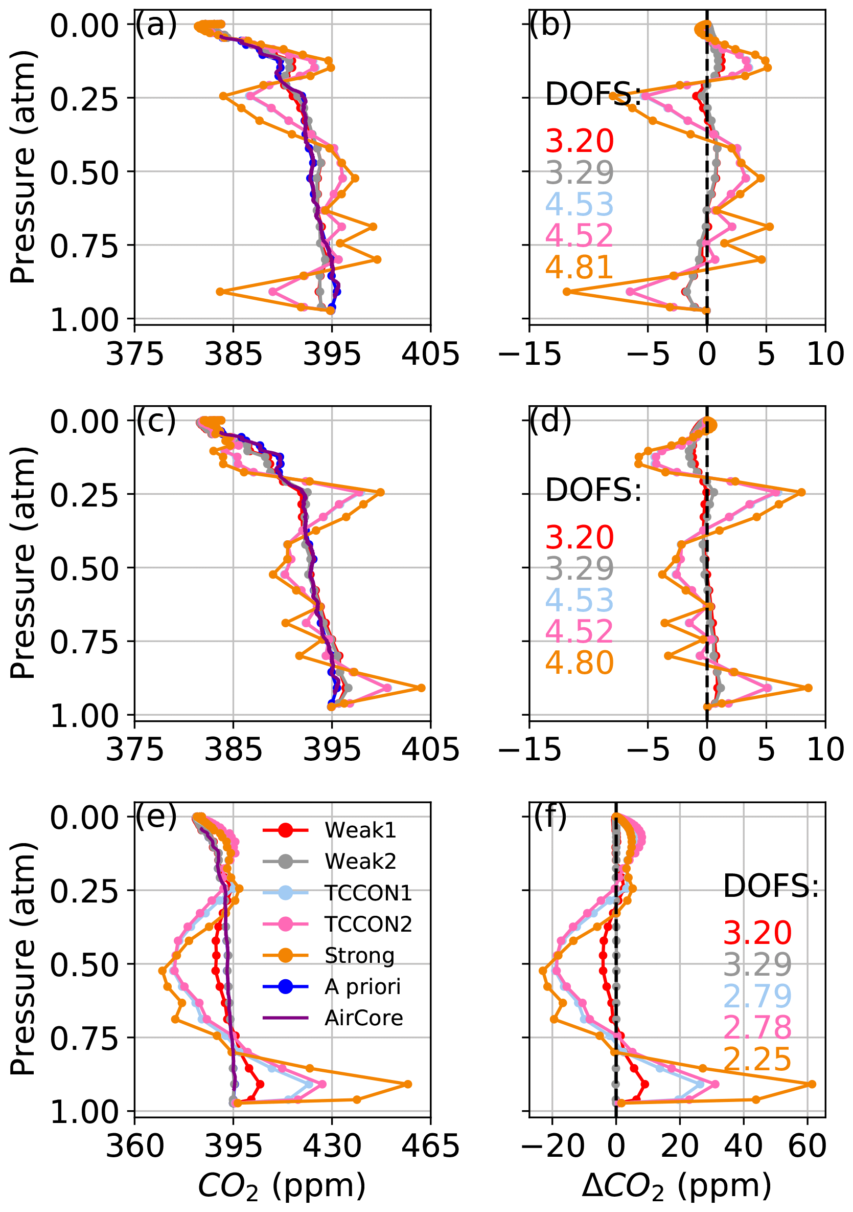
Figure 7 The left-hand panels show CO₂ profiles retrieved using synthetic spectra. In (a) the air- and self-broadened half-width coefficients of all CO₂ lines is increased by 0.1 %. In (c) the temperature dependence of these coefficients is decreased by 1 %. In (e), the synthetic spectrum used as “measurement” is generated with the speed-dependent Voigt line shape with line mixing, but profiles are retrieved using a Voigt line shape. Panels (b), (d), and (f) show the difference between the retrieved profiles and AirCore, corresponding to (a), (c), and (e) respectively.

Figure 8 Panel (a) shows an example of calculated lines in the Strong CO₂ window. The other panels show residuals from fits to a synthetic spectrum, using the same inputs used to generate the synthetic spectrum except for (b) no perturbation; (c) +2 ^∘C perturbation to the a priori temperature between 8 and 13 km; (d) a CO₂ prior profile set to 380 ppm at all levels, corresponding to ∼ 15 ppm offset from the unperturbed prior; (e) air- and self-broadened Lorentz half-width coefficients increased by 0.1 %; (f) temperature dependence of the half-width coefficients decreased by 1 %; and (g) using the a priori profiles that would be used by TCCON operational processing, instead of that constructed from in situ measurements, resulting in a combination of different errors in the a priori profiles such as H₂O, temperature, and CO₂. Note the vertical scale of panels (b), (e), and (f) is 5 times smaller than that of panels (c), (d), and (g).

A factor of 10 increase in the perturbations applied to the width coefficients or their temperature dependence also leads to a factor of 10 increase in the amplitude of deviations in the retrieved CO₂ profiles. Figure 7a and b use perturbations corresponding to uncertainties in the line parameters when using qSDV+LM for the TCCON windows and the Strong window. The same perturbations were applied for all five windows. However, in the Weak1 and Weak2 windows, these perturbations are 10 times smaller than realistic uncertainties as reported in Table 4 for the Voigt line shape. Therefore, for the Weak windows, we can expect deviations from the truth 10 times larger than in Fig. 7, within ∼ 10–20 ppm.

In Connor et al. (2016), the authors used a Voigt line shape. Figure 7e shows the effect of fitting with a Voigt line shape a synthetic spectrum that was generated using qSDV+LM. In that case the fit residuals in the Strong window can exceed 1 % and the residuals in the TCCON windows can exceed 0.5 %. For these retrievals, the SNR is set to 100 in the Strong window, 200 in the TCCON windows, and 1000 in the Weak windows. The profiles retrieved from the Strong window present deviations from the truth within 60 ppm. In the two TCCON windows, the deviations from the truth are within 30 ppm. In the Weak1 window, the deviations from the truth are within 10 ppm, because qSDV+LM was not used to calculate the CO₂ line absorptions themselves, but only for the relatively strong CH₄ lines in that window. In the Weak2 window, there is no difference between the two line lists or line shape, and thus the retrieved profile does not differ from the a priori profile. Therefore, even if we assume perfect a priori meteorology, the deviations in the CO₂ profiles retrieved from the TCCON1 window observed by Connor et al. (2016) when fitting real spectra could be entirely due to the use of the Voigt line shape.

The effect of the errors in the a priori water vapor and temperature profiles and in the spectroscopic parameters cannot be mitigated by adjusting the measurement covariance, for example by using a variable SNR. Figure 8 shows an example of spectral residuals from fits to synthetic spectra from the Strong window using scaling retrievals, but with different perturbations applied. Showing residuals from scaling retrievals reveals systematic features that the profile retrieval will attempt to suppress. Figure 8b presents residuals from fitting a synthetic spectrum using the same a priori profile that was used to generate the synthetic spectrum. It shows small (< 0.05 %) residuals, caused by the use of a constant ILS across the window for a faster convolution of the spectrum with the ILS. The corresponding profiles are shown in Fig. 4a. In Fig. 8c, a 2 ^∘C offset is applied to the a priori temperature profile between 8 and 13 km before fitting the synthetic spectrum. In Fig. 8d, a constant a priori CO₂ profile is used to fit a synthetic spectrum that was generated with an AirCore CO₂ profile as an a priori profile. In Fig. 8e, the air- and self-broadened Lorentz half-width coefficients are increased by 0.1 % compared to the parameters used to generate the synthetic spectrum. In Fig. 8f, the temperature dependence of the air- and self-broadened Lorentz half-width coefficients is decreased by 1 % compared to the parameters used to generate the synthetic spectrum. In Fig. 8g, the GGG2020 a priori meteorology and trace gas profiles are used as a priori profiles instead of the a priori profiles constructed with AirCore profiles used to generate the synthetic spectrum.

In all panels of Fig. 8 except panels (c) and (g), all the residual features correspond to CO₂ absorption lines. In Fig. 8c, with a perturbation to the a priori temperature profile, there is an added contribution of temperature errors on interfering species. Furthermore, the residuals in Fig. 8g result from a combination of errors in the a priori meteorology and trace gas profiles but are dominated by temperature errors. Perturbations in the temperature profile, CO₂ profile, or CO₂ line width coefficients all cause residuals with the same shape because they all affect the width of CO₂ lines. It is not possible to de-weight the effect of any of those errors by adjusting the measurement error without also losing the ability to correct for residuals caused by CO₂ errors. Residuals caused by realistic temperature errors as shown in Fig. 8c are of the same magnitude as those caused by unrealistically high errors in the a priori CO₂ profile shape as shown in Fig. 8d.

3.1.5 Synthetic spectra: discussion

For retrievals on synthetic spectra, the “measurement” SNR is set to 1000, which is high compared to most solar spectra measured by TCCON. So in profiles retrieved from real spectra, we can expect a greater influence of the a priori CO₂ profile: the deviations will be smaller, and the degrees of freedom for signal will be lower than those shown in the figures of Sect. 3.1. This is not a desirable outcome; the a priori CO₂ covariance is meant to nudge the retrieval such that the solution lies close to realistic ensembles of CO₂ profiles, not to constrain deviations caused by temperature errors. Tuning the a priori or measurement covariances is not the right approach until profile deviations caused by typical errors in spectroscopy or meteorology are smaller than typical vertical variations in CO₂ profiles. Figure 4 shows that the profile retrieval algorithm works well and could be a powerful tool to derive information about the vertical distribution of CO₂, even with ill-defined a priori CO₂ profiles. Panels (a) and (b) of Fig. 7 show that profile information could still be retrieved to within ∼ 5 ppm given realistic errors in line width parameters. But as shown with Fig. 6, a temperature retrieval, or correction, is critical to producing reliable CO₂ profile retrievals. This study does not show the effect of typical instrument misalignment errors on the retrieved profiles. GFIT2 currently has no capacity to fit the instrument line shape (ILS) of a misaligned instrument given specific angular and shear misalignments and instead always assumes a perfect ILS. This is an area of future development for the program. The effect of an error in the instrument's internal field of view and the effect of a zero-level offset are presented in Appendix F; both should lead to minor deviations from the truth, within less than 3 ppm.

In Sect. 3.2, GFIT2 is tested with real spectra using an a priori profile built from in situ measurements. In that case, the deviations from the truth in the retrieved CO₂ profile caused by errors in the a priori meteorology (temperature, pressure, and water vapor profiles) are minimized, and the remaining deviations are caused by errors in the spectroscopic line parameters, in the radiative transfer, in the instrument line shape, or in the pointing of the sun tracker.

3.2 Real spectra

Here the algorithm is tested with real spectra measured at Lamont as described in Sect. 2.2. A scaling retrieval is performed before each profile retrieval and the root mean square of the residuals from the scaling retrieval is used as measurement uncertainty for the profile retrieval. Since the residuals from the scaling retrieval include systematic features larger than the random noise in the measurement, the root mean square is a conservative estimate of the noise. In Sect. 3.2.1, we present CO₂ profiles retrieved from real spectra and we attempt to isolate the effect of errors in instrument line shape, in spectroscopic parameters, and in pointing, from the effect of errors in meteorology. In Sect. 3.2.2, we present an analysis of the information content and altitude sensitivity of the retrieval. Finally, in Sect. 3.2.3, we compare XCO₂ derived from the scaling retrieval to XCO₂ derived from the profile retrieval.

3.2.1 Profiles

Figures 9 and 10 show CO₂ profiles retrieved from real spectra measured from Lamont, OK, on 14 January 2012 and 11 April 2017, respectively. In each figure, panel (a) shows profiles retrieved using in situ profiles (the “truth”) as the a priori profiles. In those cases, we assume that deviations from the truth caused by errors in a priori meteorology (pressure, temperature, and water vapor profiles) are minimized, and the remaining deviations can be attributed to the combination of instrument misalignment (ILS), pointing errors, or errors in spectroscopic parameters. Panel (c) shows profiles retrieved using the GGG2020 a priori profiles. A first complication for obtaining a satisfactory CO₂ profile retrieval is that the a priori CO₂ profiles in GGG2020 already compare well with in situ profiles, typically within 5 ppm over Lamont. In Figs. 9c and 10c, the profile that most closely matches the AirCore is the a priori profile.

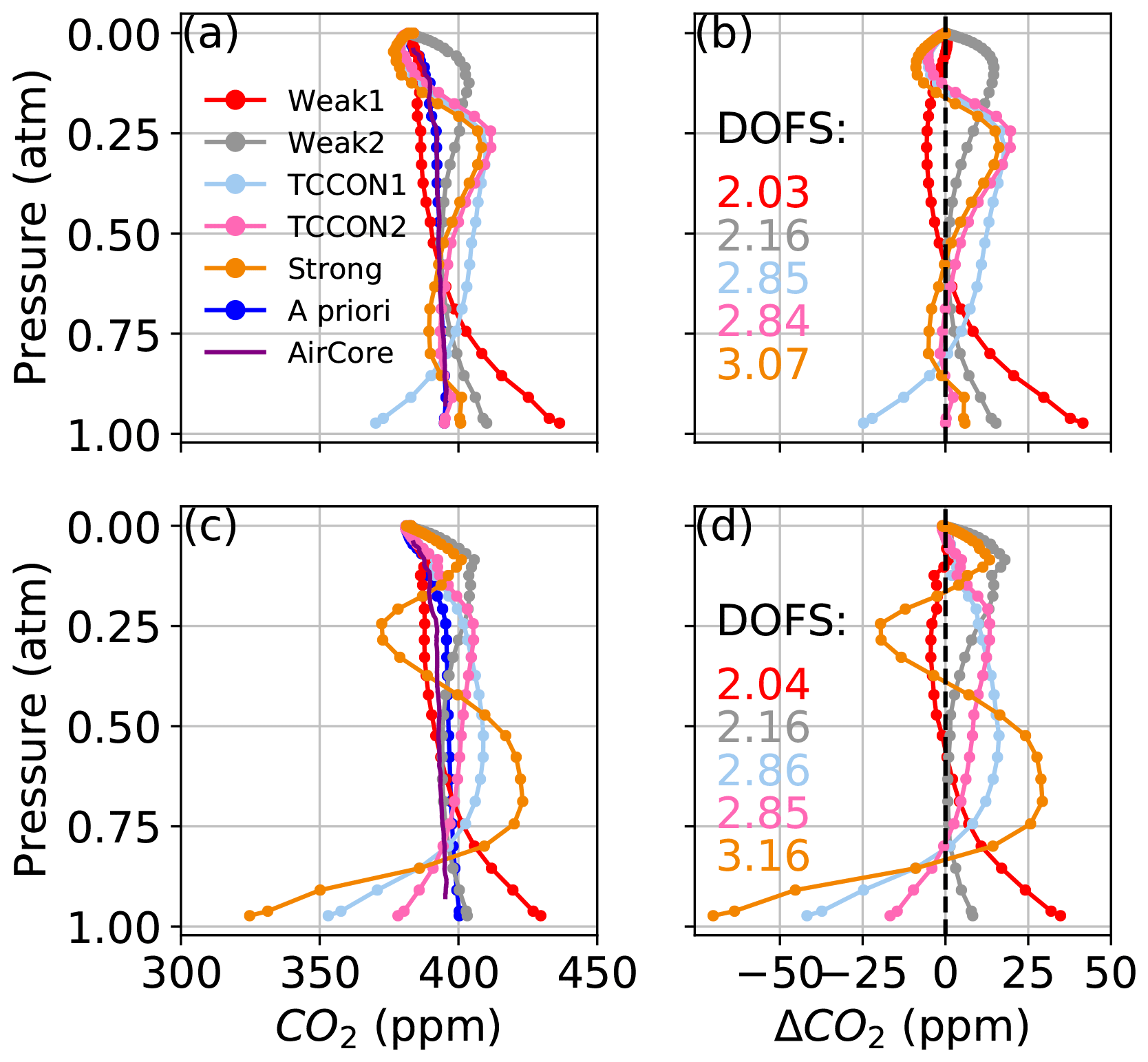
Figure 9 CO₂ profiles retrieved from spectra measured at the Lamont TCCON site on 14 January 2012, at 61–74^∘ solar zenith angle, coincident with AirCore measurements using (a) the AirCore “truth” as a priori profiles and (c) the GGG2020 a priori profiles. In (b) and (d) the difference of the retrieved profiles minus the AirCore profile is shown, corresponding to (a) and (c), respectively. The points represent the 51 levels of the vertical grid. The DOFs for each retrieval window are indicated in (b) and (d).

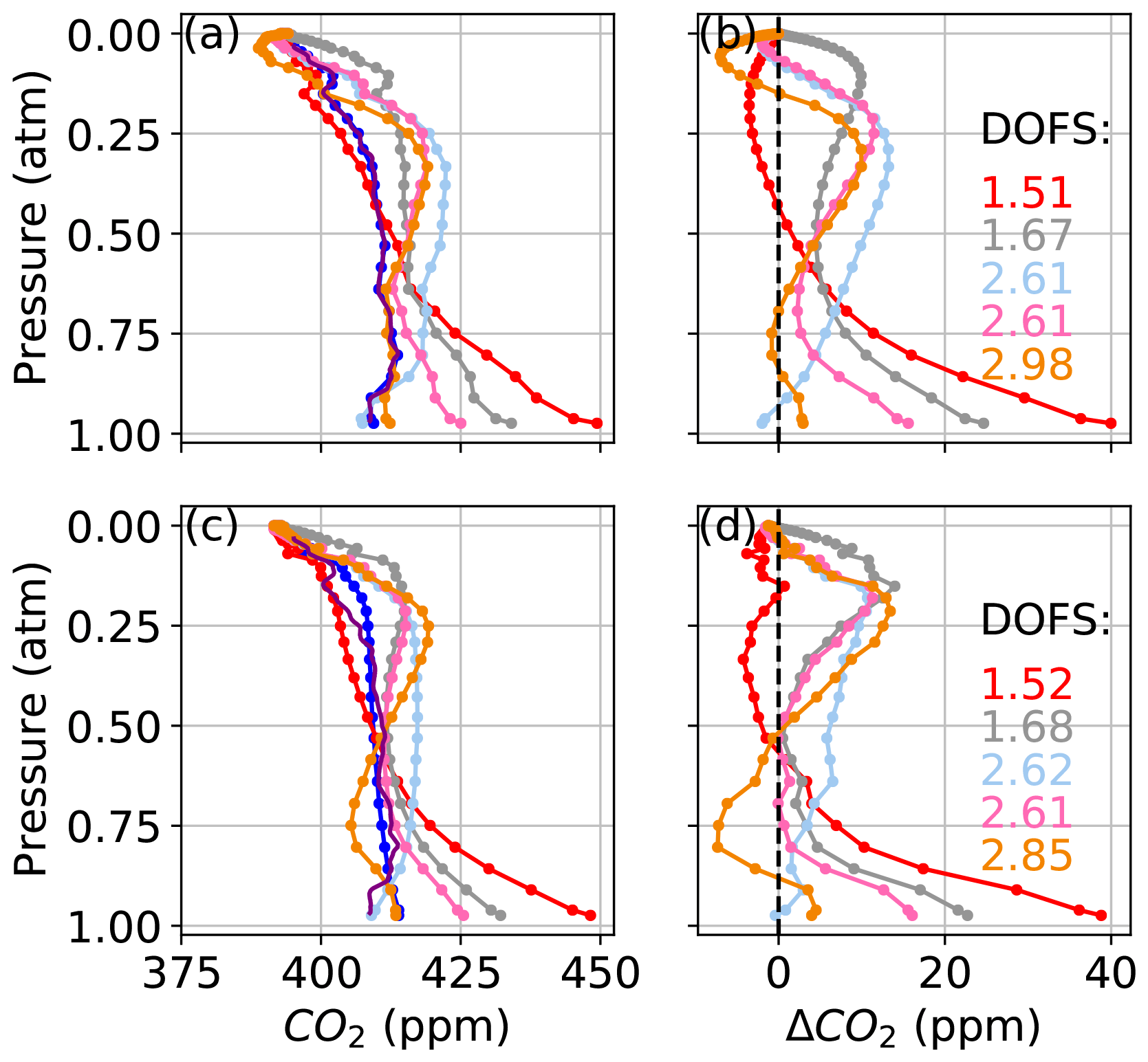
Figure 10 Same as Fig. 9 but for spectra measured on 11 April 2017 at 28–39^∘ solar zenith angle.

Even with ideal prior knowledge of the meteorology and trace gas profiles, the CO₂ deviations from the truth can be as large as 50 ppm as shown in Figs. 9a and 10a. When synthetic spectra were perturbed with realistic errors in line width parameters, profile deviations remained within 5 ppm for profiles retrieved from the Strong window and within 10 ppm for the TCCON windows. This suggests that the main cause of deviations in Figs. 9a and 10a is not due to errors in spectroscopic parameters. The assumption that there is no contribution from temperature errors in the radiosonde profile is supported by the CO₂ profile deviation being smallest in the Strong window, which is the most sensitive to temperature errors. Although the effect of typical perturbations in the instrument field of view, zero-level offset, and spectroscopic parameters is relatively small compared to the effect of temperature errors, the cumulative effect of these errors could explain the deviations from the truth in Figs. 9a and 10a.

Figure 11 shows the difference between the GGG2020 a priori temperature profile, used in Figs. 9c and 10c, and the radiosonde temperature profile used in Figs. 9a and 10a. In both cases, we replace the a priori surface temperature with the measured surface temperature. On 14 January 2012, the radiosonde temperature profile is about 1 ^∘C higher than the GGG2020 a priori profile at pressures < 0.6 atm. The shape of the Strong window CO₂ profile deviations in Fig. 9c is consistent with the sensitivity tests using synthetic spectra in Sect. 3.1.3. In Fig. 6a, a +5 ^∘C offset below 5 km results in +500 ppm CO₂ error at ∼ 0.9 atm, while in Fig. 10, a −1 ^∘C offset in the lower troposphere leads to a −50 ppm error at ∼ 0.9 atm. The deviations are smoother in Figs. 9 and 10 than in Fig. 6 because the SNR of real spectra is between 200 and 500 instead of 1000, and because of the smoothing effect of the off-diagonal elements of the a priori covariance used in this section. The off-diagonal elements of the a priori covariance introduce inter-layer correlations that reduce large differences between levels over a given length scale (see Sect. 2.2). Retrievals on real spectra after applying a +5 ^∘C offset to the radiosonde temperature profile below 5 km lead to a +100 ppm offset at ∼ 0.9 atm. The CO₂ profiles in Fig. 10c differ less with those in Fig. 10a than do the profiles in Fig. 9a and c. In Fig. 11, the difference between the GGG2020 and radiosonde temperature profile on 11 April 2017 is ∼ 3 ^∘C for the first two levels above the surface, but the average difference between 0.85 and 0.6 atm is −0.15 ^∘C compared to −1.05 ^∘C on 14 January 2012.

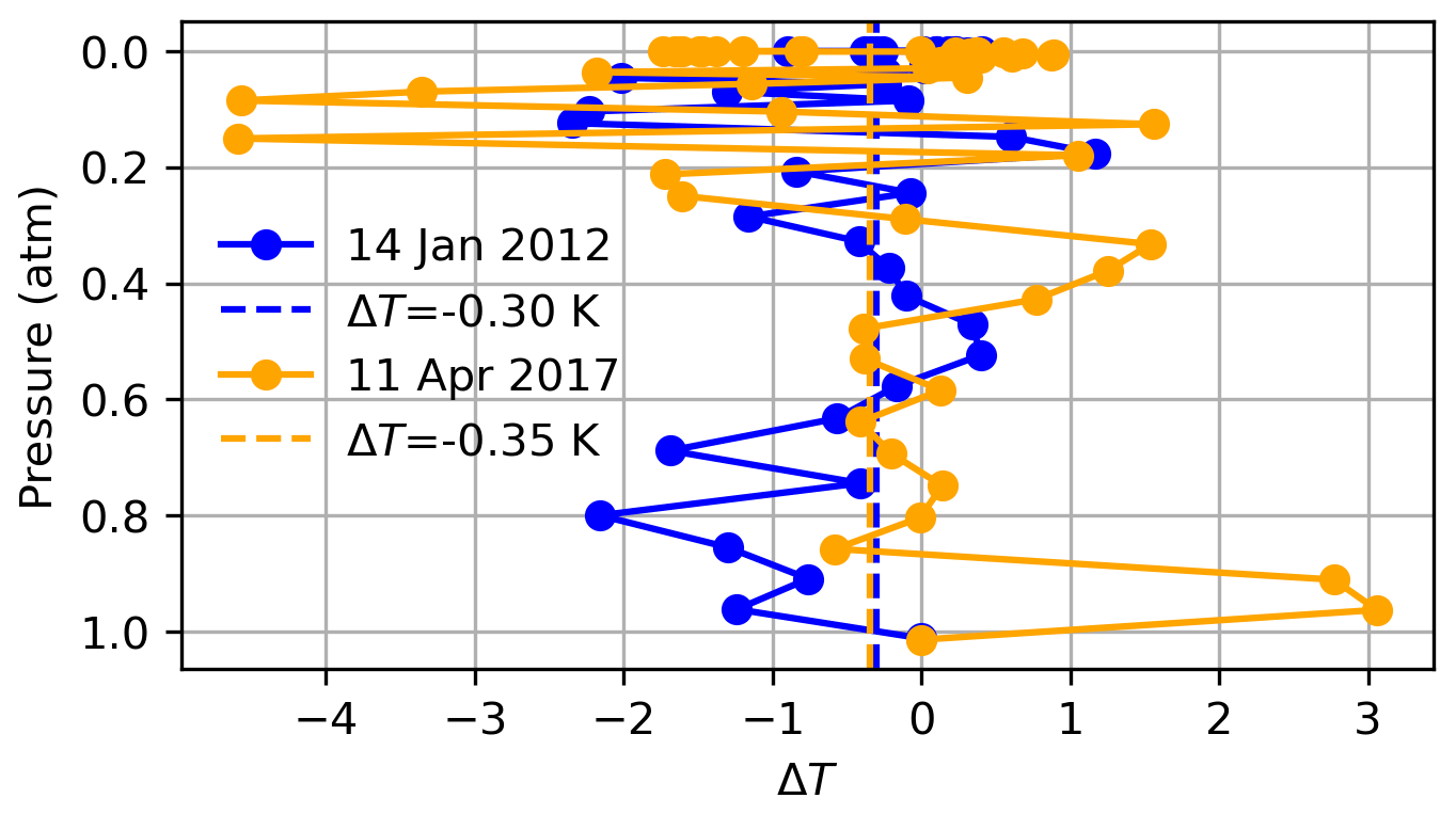
Figure 11 Temperature profile difference for the GGG2020 a priori minus radiosonde on 14 January 2012 and 11 April 2017. The radiosonde profile is included in the a priori profiles used in panel (a) of Figs. 9 and 10, and the GGG2020 a priori profiles are used in panel (b) of Figs. 9 and 10. In situ temperature measurements are used for both cases at the surface. The dashed line marks the average difference, with the value indicated in the legend.

In aircraft profiles over Lamont between 2008 and 2018 from NOAA's ObsPack, the steepest vertical gradients in CO₂ profiles are ∼ 5 ppm km⁻¹ between the surface and ∼ 3 km. In its current state, CO₂ profile retrieval with GFIT2 cannot distinguish these vertical variations from CO₂ deviations caused by errors in the forward model, even with very accurate a priori meteorology. Typical errors in the a priori temperature profiles will prevent operational use of CO₂ profile retrieval without a scheme for retrieving or correcting the temperature profiles.

3.2.2 Information content and averaging kernel

Table 5 presents the average values of the Shannon information content, H, and of the CO₂ profile DOFs, from all profile retrievals performed on Lamont spectra when using the GGG2020 a priori profiles. It also includes the ratio of residuals (RR) of the spectral fits (see Appendix B, Eq. B10), which represents the residuals of the profile retrievals as a fraction of the residuals of the scaling retrievals. The same quantities are plotted in Fig. 12 for each spectrum. The RR is always smaller than 1 because the profile retrieval has more freedom to adjust the calculated spectrum and so can never produce larger residuals than scaling retrievals. Figure 12 also shows XCO₂ obtained from the scaling retrievals subtracted to XCO₂ obtained from profile retrievals for each window.

Table 5 Shannon information content (H), degrees of freedom for signal (DOFs) for the CO₂ profile, and ratio of residuals (RR) averaged over all 492 profile retrievals from near-infrared TCCON spectra measured at Lamont and coincident within ±1 h of the AirCore last sampling time. The standard deviation is also shown.

Figure 12 Shannon information content (top left), degrees of freedom for signal for the CO₂ profile (top right), and ratio of residuals (bottom left), and profile minus scaling retrieval XCO₂ (bottom right) for all Lamont spectra coincident within ±1 h of the AirCore last sampling time for AirCores launched on the dates indicated on the right. Each new date is marked by a vertical dashed line.

Figure 13 shows the sums of the rows of the partial column averaging kernel matrix over different altitude ranges. The sum from 0 to 70 km is the total column averaging kernel (see Appendix C). The total column averaging kernel is close to 1 at all levels in all windows, indicating good sensitivity to changes in the CO₂ total column. The partial column kernels show that most of this sensitivity comes from altitudes below 15 km. That the total column averaging kernel is close to 1 at all levels is not inconsistent with the large deviations we observe in the retrieved CO₂ profiles. If the total column averaging kernel is exactly one at each level, adding N molecules of CO₂ anywhere in the atmosphere will lead to N more molecules in the retrieved total column. However, in the presence of a priori temperature errors, for example, the retrieved value can be biased. The averaging kernel indicates that without the effect of these errors, the CO₂ profile retrieval would have excellent sensitivity to CO₂ and would be able to provide information about CO₂ in two distinct layers. Here, the vertical representation is not a concern. Using 51 vertical levels only affects the speed of the retrieval. The retrieved profiles can then be reduced to a number of partial columns corresponding to the DOFs. This was not done here because it is evident that large deviations due to temperature errors could easily bias the resulting partial columns. The reduction into a subset of layers also requires an arbitrary choice: in Fig. 13 the altitude ranges were set such that the DOFs of the first two partial columns would be roughly close to 1 in each window. We could also have chosen two regions with approximately equal DOFs from 0–7 and 7–70 km. The partial column averaging kernels overlap with each other, so the partial columns are not completely uncorrelated even if their respective DOFs are higher than 1. The DOFs are not exactly independent pieces of information, as it is impossible to obtain independent partial column amounts from direct-sun measurements on the ground (see Appendix C), but an arbitrary criterion can be defined to identify distinct layers, for example if the peaks in their partial column averaging kernels are separated by a given fraction of their widths in altitude. Additional analysis of the vertical sensitivity of the retrieval is presented in Appendix D, as well as a decomposition of the retrieval error into the interference, measurement noise, and smoothing errors as shown in Fig. D8. The interference error is the smallest (< 0.5 %) contribution but does not include the effect of temperature errors. The measurement noise error decreases from ∼ 1 % at the surface to ∼ 0.2 % at pressures less than 0.6 atm (> 5 km), and the smoothing error dominates and decreases roughly from ∼ 3 % at the surface to 1 % at the top of the atmosphere.

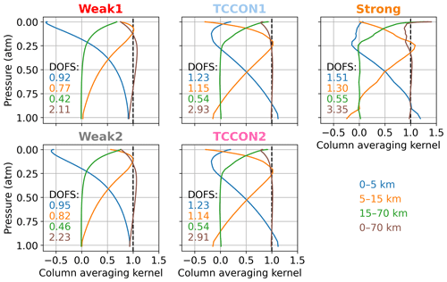
Figure 13 Sum of the rows of the partial column averaging kernel matrix over different altitude ranges as indicated by the legend, for each of the five CO₂ windows. The sum between 0–70 km is the total column averaging kernel. The numbers in each panel are the DOFs corresponding to each of the altitude ranges.

3.2.3 XCO₂

The XCO₂ derived from profile and scaling retrievals using the GGG2020 a priori profiles was compared to XCO₂ derived from the CO₂ profile built from the AirCore CO₂ profile, in situ surface measurements of CO₂, and the GGG2020 a priori CO₂ above the maximum altitude sampled by the AirCore. The results are shown in Fig. 14 for the 8 days we have AirCore profiles that are coincident with measurements at the Lamont TCCON station. Despite the large deviations observed in retrieved profiles, the XCO₂ derived from profile retrievals compares well to the AirCore XCO₂, but it does not present a clear improvement over the XCO₂ derived from the scaling retrievals. The effect of temperature errors on XCO₂ derived from scaling and profile retrievals is relatively small because the spectral windows utilize the entire (fundamental) band. Across a wide window, the residuals due to temperature errors show alternating positive and negative residuals, because of the different temperature sensitivities of absorption lines. Collectively, these lines have a small net temperature sensitivity. The scaling retrieval, which can only add or remove CO₂ at all levels simultaneously, is limited in its ability to fit out such residuals across a wide window by adjusting the CO₂ scale factor. For profile retrievals, although large deviations are observed in the retrieved profile, they compensate each other when deriving the total column. These deviations compensate due to the wide windows including a range of spectral lines with different temperature sensitivities. If a narrow window over only a few lines were used instead, we would expect more localized errors in the retrieved CO₂ profiles, and total columns sensitive to temperature errors.

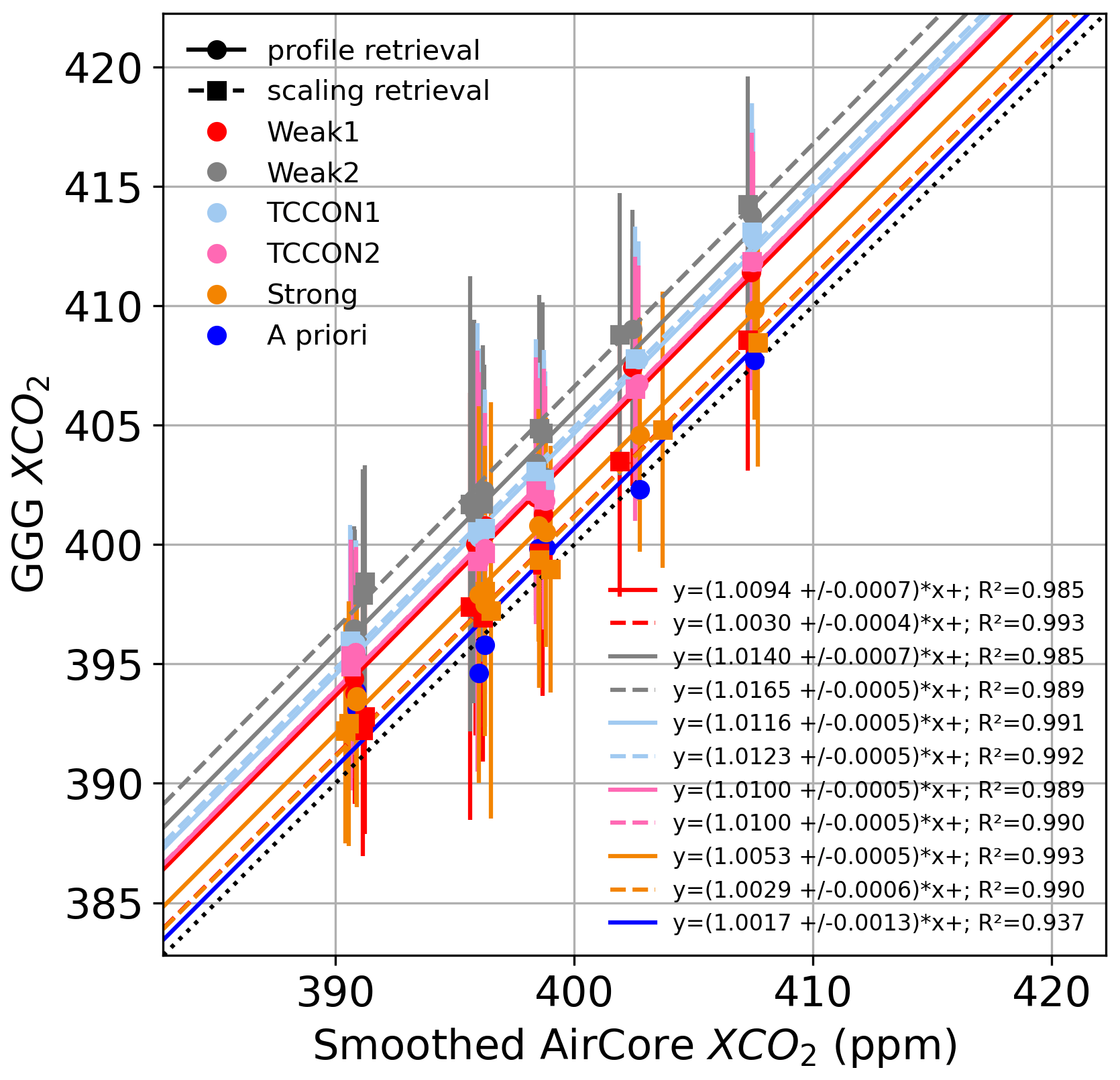
Figure 14 XCO₂ derived from scaling (dashed lines and squares) and profile (solid lines and circles) retrievals for each CO₂ window when using the GGG2020 a priori profiles, compared to XCO₂ derived from smoothed AirCore profiles (see Appendix C). The black dotted line marks the 1-to-1 line. When comparing with scaling retrievals, the AirCore profile is smoothed using the total column averaging kernel of the scaling retrieval, and when comparing to profile retrievals the AirCore profile is smoothed using the averaging kernel matrix of the profile retrieval. The legend indicates the slopes and squared Pearson correlation coefficients of fits to lines passing through the origin, assuming that in the absence of CO₂ the retrieval would return a CO₂ value of zero.

3.2.4 Real spectra: discussion

Profile retrievals that use real spectra and an a priori profile built from coincident in situ measurements show CO₂ profile deviations up to 40–50 ppm. Even when the errors due to the a priori meteorology are minimized, deviations from the truth due to instrument misalignment, radiative transfer, sun-tracker pointing, or uncertainties in line parameters are larger than the steepest vertical CO₂ gradients (∼ 5 ppm km⁻¹) observed in the ensemble of aircraft profiles from NOAA's ObsPack.

When performing retrievals on the same spectra but replacing the AirCore a priori profile with a standard a priori profile, small errors in the a priori temperature profile cause large deviations in the retrieved CO₂ profile. Despite the large deviations in the retrieved profiles, the retrieval still shows high sensitivity to XCO₂ but does not present a clear improvement over XCO₂ obtained from scaling retrievals. Introducing a temperature retrieval or correction, as well as the ability to model an imperfect instrument line shape, is the best avenue to improve the CO₂ profile retrieval results. Appendix E presents an attempt at applying empirical corrections to reduce the effect of systematic imperfections in the forward model.

4 Summary and conclusions

In this study we investigated the use of CO₂ profile retrievals from near-infrared solar absorption spectra measured by TCCON. The performance of CO₂ profile retrieval was reassessed after improvements were implemented in the forward model of GGG. Retrievals were performed using five CO₂ windows with significantly different optical opacities.

We first use retrievals on synthetic spectra to check the self-consistency. Typical errors in the a priori H₂O profile, which is retrieved with a scaling retrieval, caused limited deviations from the truth in the CO₂ profile, within 5–10 ppm in the Strong window, and within 2 ppm in the other windows. Perturbing the CO₂ air- and self-broadened Lorentz half-width coefficients and their temperature dependence to within their estimated uncertainties led to CO₂ deviations from the truth of less than 5 ppm. The implementation of a non-Voigt line shape is a significant improvement to CO₂ profile retrievals; errors in spectroscopic parameters are no longer the leading source of uncertainty in retrieved profiles. We observed deviations from the truth of up to 100 ppm in profiles retrieved with typical temperature errors. The temperature profile is an important retrieval input but is not retrieved; thus spectral residuals caused by errors in the a priori temperature profile are free to be suppressed by adjustments to the CO₂ scale factors. The implementation of a temperature profile retrieval, or correction, is critical to improve CO₂ profile retrieval results. In GGG2020, 3-hourly a priori temperature profiles are used, but temperatures can still vary by several degrees between 3-hourly profiles and can still be wrong even without any time mismatch. Temperature could be retrieved from CO₂ windows and from windows with temperature-sensitive water vapor absorption lines.

We then perform retrievals with atmospheric TCCON spectra collected at the Lamont site, which were coincident with AirCore profiles, including radiosonde profiles of temperature and relative humidity; these were considered as the true state of the atmosphere. When running retrievals with the truth as the a priori profiles, the deviations due to errors in the a priori meteorology are minimized and the resulting deviations are caused by instrument misalignment, errors in spectroscopy, or sun tracker pointing. We observed CO₂ deviations of up to 40 ppm in that case. Even with ideal knowledge of the a priori meteorology, the CO₂ deviations are larger than the largest expected vertical CO₂ variations and no useful profile information can be inferred from the profile retrieval. Stricter alignment requirements, which can be challenging to achieve in practice, or the ability to model an imperfect instrument line shape are needed to improve profile retrieval results. The sensitivity study of Sect. 3.1 could then be extended to assess the effect of specific misalignments on the retrieved profiles.

In these retrievals, we used a full a priori covariance matrix, with off-diagonal elements, based on comparisons between the GGG2020 a priori and aircraft vertical profiles from NOAA's ObsPack over the Lamont TCCON site. Before tuning the a priori covariance and considering stronger regularizations, it must be shown that CO₂ deviations caused by typical errors in the a priori meteorology are smaller than typical variability in real CO₂ profiles. Because it is more computationally expensive, and because it requires stronger constraints on the a priori statistics than scaling retrievals, a profile retrieval must present clear advantages over a scaling retrieval to justify its operational use. And with each new improvement to the CO₂ a priori profiles, requirements for profile retrieval to be better than scaling retrieval become more stringent.

A method to combine the profiles obtained from sequential retrievals in different spectral windows still needs to be developed. Alternatively, the ability to perform simultaneous retrievals using multiple spectral windows could be implemented in GFIT2.

Appendix A: Vertical columns

The vertical grid for the retrievals presented in this study has 51 levels from 0 to 70 km, with spacing increasing with altitude and following:

$$\begin{array}{}\text{(A1)}& z_i=i\times \left(\mathrm{0.4}+\mathrm{0.02}\times i\right),\end{array}$$

where z_i is the altitude in kilometers of the ith level. Each level is associated with an effective vertical path distance vp:

$$\begin{array}{}\text{(A2)}& {\mathrm{vp}}_i\approx \mathrm{0.4}+\mathrm{0.04}\times i.\end{array}$$

The total column of air in molecules per square meter can be obtained as

$$\begin{array}{}\text{(A3)}& {\mathrm{column}}_{\mathrm{Air}}=\sum _{i=\mathrm{1}}^N{\mathrm{vp}}_i\times d_i,\end{array}$$

where d is the air number density in molecules of air per cubic meter. N is the number of atmospheric levels. If the prescribed grid contains layers below the altitude of the site considered, their effective vertical path will be 0. The layer containing the site altitude will be truncated. The total column of CO₂ is

$$\begin{array}{}\text{(A4)}& {\mathrm{column}}_{{\mathrm{CO}}_{\mathrm{2}}}=\sum _{i=\mathrm{1}}^N{\mathrm{sf}}_i\times {\mathrm{vmr}}_i\times d_i\times {\mathrm{vp}}_i,\end{array}$$

where sf is the retrieved scaling factor and vmr is the a priori CO₂ wet mole fraction (molecules of CO₂ per molecules of air). In the forward model, the retrieval grid is not vertical, but along the slant path from the instrument towards the sun, the scaling factors retrieved for the slant layers are used with the corresponding vertical layers to compute the vertical column. The a priori profiles used by GFIT are built on the prescribed altitude grid directly above the site. This should contribute to an unknown error, largest at high solar zenith angles when the projection of the sun ray on the ground can reach a few hundred kilometers; in that case the a priori slant profiles of temperature and H₂O could be significantly different from the vertical profile directly above the instrument.

The column-averaged dry-air mole fraction of CO₂ (XCO₂) is the ratio of the column of CO₂ to the column of dry air, where the column of dry air is expressed as the column of O₂ divided by 0.2095 (Wunch et al., 2011b):

$$\begin{array}{}\text{(A5)}& {\mathrm{XCO}}_{\mathrm{2}}=\mathrm{0.2095}\times {\displaystyle \frac{\stackrel{\mathrm{‾}}{{\mathrm{column}}_{{\mathrm{CO}}_{\mathrm{2}}}}}{{\mathrm{column}}_{{\mathrm{O}}_{\mathrm{2}}}}},\end{array}$$

where the O₂ column is retrieved from a spectral window centered at 7885 cm⁻¹. For the official TCCON products, $\stackrel{\mathrm{‾}}{{\mathrm{column}}_{{\mathrm{CO}}_{\mathrm{2}}}}$ is a weighted average of the columns retrieved from the TCCON1 and TCCON2 windows.

Appendix B: GFIT2 algorithm

To find the state vector with maximum a posteriori probability given a measurement, the cost function J is minimized,

$$\begin{array}{}\text{(B1)}& \begin{array}{rl}J& ={\left(\mathbf{y}-f\left(\mathit{x}\right)\right)}^T{\mathbf{S}}_y^{-\mathrm{1}}\left(\mathbf{y}-f\left(\mathit{x}\right)\right)\\ & +{\left({\mathit{x}}_{\mathrm{a}}-\mathit{x}\right)}^T\mathbf{R}\left({\mathit{x}}_{\mathrm{a}}-\mathit{x}\right),\end{array}\end{array}$$

by iteratively solving for the state update Δx in the least square problem:

$$\begin{array}{}\text{(B2)}& \begin{array}{rl}\left({\mathbf{K}}_i^T{\mathbf{S}}_y^{-\mathrm{1}}{\mathbf{K}}_i+\mathbf{R}+\mathit{\gamma }\mathbf{D}\right)\mathrm{\Delta }\mathit{x}& ={\mathbf{K}}_i^T{\mathbf{S}}_y^{-\mathrm{1}}\left(\mathbf{y}-f\left({\mathit{x}}_i\right)\right)\\ & +\mathbf{R}\left({\mathit{x}}_{\mathrm{a}}-{\mathit{x}}_i\right).\end{array}\end{array}$$

Here, y is the measured transmittance spectrum, f is the forward model that computes a transmittance spectrum from the state vector x, S_y is the measurement covariance matrix, x_a is the a priori state vector, and the regularization matrix R is taken to be the inverse of the a priori covariance matrix S_a. K is the Jacobian matrix, and each column of K contains the derivative of the spectrum with respect to an element of the state vector, $\mathbf{K}=\frac{\partial f\left(x\right)}{\partial x}$. The Levenberg–Marquardt parameter γ is applied to a scaling matrix D, which is also taken to be ${\mathbf{S}}_{\mathrm{a}}^{-\mathrm{1}}$. The Levenberg–Marquardt parameter affects the size of the state update so that smaller steps may be taken when the linearization of the forward model is not satisfactory.

The expected χ² of the maximum a posteriori probability solution should be

$$\begin{array}{}\text{(B3)}& {\mathit{\chi }}^{\mathrm{2}}\left(\widehat{x}-\mathit{x}\right)={\left(\widehat{x}-\mathit{x}\right)}^T\left({\mathbf{K}}^T{\mathbf{S}}_y^{-\mathrm{1}}\mathbf{K}+{\mathbf{S}}_{\mathrm{a}}^{-\mathrm{1}}\right)\left(\widehat{x}-\mathit{x}\right)\approx n,\end{array}$$

where n is the number of state vector elements. A solution is accepted when the ratio of the squared state update to the estimated variance is a negligible fraction of the expected χ²:

$$\begin{array}{}\text{(B4)}& \mathrm{\Delta }\mathit{x}\left({\mathbf{K}}^T{\mathbf{S}}_y^{-\mathrm{1}}\left(\mathbf{y}-f\left({\mathit{x}}_i\right)\right)+{\mathbf{S}}_{\mathrm{a}}^{-\mathrm{1}}\left({\mathit{x}}_{\mathrm{a}}-{\mathit{x}}_i\right)\right)\ll n.\end{array}$$

In an algorithm, “≪n” must use a specific limit, and in GFIT2, “$<n/\mathrm{10}$” was used. If the inequality check is made with a parameter that is too large, like “<n”, the algorithm may take fewer iterations to converge but will take the same steps at each iteration, often leading to a retrieved profile closer to the a priori profile. The inequality check should be done with a small enough fraction of n that reducing it further does not significantly affect the solution.

If convergence is not reached in the ith iteration, an algorithm determines if the Levenberg–Marquardt parameter needs to be adjusted for the next iteration (Fletcher, 1971). Three different cost functions are used:

$$\begin{array}{}\text{(B5)}& {\displaystyle }\begin{array}{rl}{J}_{\mathrm{old}}& ={\left(\mathbf{y}-f\left({\mathit{x}}_i\right)\right)}^T{\mathbf{S}}_y^{-\mathrm{1}}\left(\mathbf{y}-f\left({\mathit{x}}_i\right)\right)\\ & +{\left({\mathit{x}}_{\mathrm{a}}-{\mathit{x}}_i\right)}^T{\mathbf{S}}_{\mathrm{a}}^{-\mathrm{1}}\left({\mathit{x}}_{\mathrm{a}}-{\mathit{x}}_i\right),\end{array}\text{(B6)}& {\displaystyle }\begin{array}{rl}{J}_{\mathrm{new}}& ={\left(\mathbf{y}-f\left({\mathit{x}}_i+\mathrm{\Delta }\mathit{x}\right)\right)}^T{\mathbf{S}}_y^{-\mathrm{1}}\left(\mathbf{y}-f\left({\mathit{x}}_i+\mathrm{\Delta }\mathit{x}\right)\right)\\ & +{\left({\mathit{x}}_{\mathrm{a}}-{\mathit{x}}_i-\mathbf{\Delta }\mathit{x}\right)}^T{\mathbf{S}}_{\mathrm{a}}^{-\mathrm{1}}\left({\mathit{x}}_{\mathrm{a}}-{\mathit{x}}_i-\mathrm{\Delta }\mathit{x}\right),\end{array}\text{(B7)}& {\displaystyle }\begin{array}{rl}{J}_{\mathrm{pred}}& ={\left(\mathbf{y}-f\left({\mathit{x}}_i\right)-\mathbf{K}\mathrm{\Delta }\mathit{x}\right)}^T{\mathbf{S}}_y^{-\mathrm{1}}\left(\mathbf{y}-f\left({\mathit{x}}_i\right)-\mathbf{K}\mathrm{\Delta }\mathit{x}\right)\\ & +{\left({\mathit{x}}_{\mathrm{a}}-{\mathit{x}}_i-\mathbf{\Delta }\mathit{x}\right)}^T{\mathbf{S}}_{\mathrm{a}}^{-\mathrm{1}}\left({\mathit{x}}_{\mathrm{a}}-{\mathit{x}}_i-\mathrm{\Delta }\mathit{x}\right),\end{array}\end{array}$$

where J_old is the cost function using the state vector at the beginning of the ith iteration, J_new is the cost function using the updated state vector at the end of the ith iteration, and J_pred is the cost function using the state vector update and the linear approximation:

$$\begin{array}{}\text{(B8)}& f\left(\mathit{x}+\mathrm{\Delta }\mathit{x}\right)\cong f\left(\mathit{x}\right)+\mathbf{K}\mathrm{\Delta }\mathit{x}.\end{array}$$

The ratio r is then evaluated:

$$\begin{array}{}\text{(B9)}& r={\displaystyle \frac{J_{\mathrm{new}}-J_{\mathrm{old}}}{J_{\mathrm{pred}}-J_{\mathrm{old}}}}.\end{array}$$

This is the relative change in the cost function produced by a state vector update when using the forward model and a linear approximation of the forward model. The Levenberg–Marquardt parameter is then adjusted as follows:

• r> 0.75. The linearization of the forward model is satisfactory and γ is reduced to allow larger steps.

  • $\mathit{\gamma }=\frac{\mathit{\gamma }}{\mathrm{2}}$

• r≥0.25. Intermediate case, make no change to γ and reset the number of consecutive divergences.

  • ndiv = 0

• r< 0.25. The linearization of the forward model is not satisfactory, increment the number of consecutive divergences, γ is increased to take smaller steps.

  • ndiv = ndiv + 1

  • if γ=0 then γ=1

  • if γ>0 then γ=10γ

If ndiv reaches some specified maximum number, there will not be another iteration. When r< 0.25, it means that the linearization of the forward model is not good enough. In GFIT2, this was not allowed to happen more than twice in a row. Increasing γ will lead to a smaller step for the state vector update, increasing the chance that the linearization of the forward model at the next step will be better and r≥0.25.

In GFIT2 r>0.75 in most cases, and if γ is not initially set to 0 it will tend towards zero until the convergence criterion is met; thus the initial value of γ was set to 0. However, the increase of the parameter is often triggered when fitting noisier spectra and can give the algorithm a chance to converge when it would otherwise need more iterations or fail without γ.

After the last iteration, the goodness of the retrieval is checked by evaluating the reduced χ² of the spectral residuals.

$$\begin{array}{}\text{(B10)}& {\mathit{\chi }}_{\mathrm{red}}^{\mathrm{2}}\left(\mathbf{y}-f\left(\mathit{x}\right)\right)={\displaystyle \frac{\mathrm{1}}{N}}\sum _{i=\mathrm{1}}^N{\left({\displaystyle \frac{{\mathbf{y}}_i-f{\left(\mathit{x}\right)}_i}{y_{\mathrm{noise}}}}\right)}^{\mathrm{2}},\end{array}$$

where y_noise is the measurement uncertainty, and N is the number of spectral points. Profile retrievals from real spectra are presented in Sect. 3 where the root mean square of the residuals from a scaling retrieval is used as y_noise. In that case Eq. (B10) is the average ratio of residuals (RR) between the profile and scaling retrieval.

The retrieval covariance matrix is

$$\begin{array}{}\text{(B11)}& \widehat{\mathbf{S}}={\left({\mathbf{K}}^T{\mathbf{S}}_y^{-\mathrm{1}}\mathbf{K}+{\mathbf{S}}_{\mathrm{a}}^{-\mathrm{1}}\right)}^{-\mathrm{1}}.\end{array}$$

The square root of its diagonal elements is used as the uncertainty in the retrieved scaling factors.

Appendix C: Averaging kernel

The state vectors of GFIT and GFIT2 contain scaling factors to be applied to a priori mole fractions. The averaging kernel matrix is

$$\begin{array}{}\text{(C1)}& \mathbf{A}={\left({\mathbf{K}}^T{\mathbf{S}}_y^{-\mathrm{1}}\mathbf{K}+{\mathbf{S}}_{\mathrm{a}}^{-\mathrm{1}}\right)}^{-\mathrm{1}}{\mathbf{K}}^T{\mathbf{S}}_y^{-\mathrm{1}}\mathbf{K}.\end{array}$$

It is a change in the retrieved state for a change in the state vector elements.

$$\begin{array}{}\text{(C2)}& {\left({\mathbf{A}}_{\mathrm{SF}}\right)}_{i,j}={\displaystyle \frac{\mathit{\delta }{\widehat{x}}_i}{\mathit{\delta }{\mathit{x}}_j}}\end{array}$$

Even though the averaging kernel is dimensionless, its units can be written as, for example, “ppm per ppm” to indicate that it is the change at a given level for a change at a different level.

To obtain the averaging kernel in ppm per ppm,

$$\begin{array}{}\text{(C3)}& {\left({\mathbf{A}}_{\mathrm{vmr}}\right)}_{i,j}={\left({\mathbf{A}}_{\mathrm{SF}}\right)}_{i,j}{\displaystyle \frac{{\mathrm{vmr}}_i}{{\mathrm{vmr}}_j}},\end{array}$$

where vmr is the a priori mole fraction at the ith and jth levels and the partial column averaging kernel matrix in molecules cm⁻² per molecules cm⁻² is

$$\begin{array}{}\text{(C4)}& {\left({\mathbf{A}}_{\mathrm{col}}\right)}_{i,j}={\left({\mathbf{A}}_{\mathrm{SF}}\right)}_{i,j}{\displaystyle \frac{{\mathrm{vmr}}_i\times d_i\times {\mathrm{sp}}_i}{{\mathrm{vmr}}_j\times d_j\times {\mathrm{sp}}_j}},\end{array}$$

where sp denotes the widths of the slant layers along the sun ray that correspond to the altitude levels of the prescribed vertical grid. The total column averaging kernel vector can be obtained from the partial column averaging kernel matrix:

$$\begin{array}{}\text{(C5)}& {\mathbf{a}}_j=\sum _{i=\mathrm{1}}^{\mathrm{nlev}}{\left({\mathbf{A}}_{\mathrm{col}}\right)}_{i,j}.\end{array}$$

It represents the change in the total column (molecules cm⁻²) caused by a change in the partial column of the jth layer. It should ideally be equal to 1 at each level, meaning that adding N target molecules anywhere in the atmosphere will lead to N more molecules in the retrieved total column.

The averaging kernel matrix would ideally be an identity matrix, meaning that adding N molecules in the jth layer would lead to N more molecules retrieved in that layer. However, adding N molecules in the jth layer will lead to an increase in the width of CO₂ absorption lines of a spectrum observed from the ground. As illustrated for CO₂ in Fig. 2, each wavenumber is affected by the CO₂ concentration over a range of altitudes, because the spectrum observed on the ground is the product of all the spectra that would be observed at each altitude. Even if that change in line widths was the only change in the spectrum and could be fitted perfectly, it would be impossible to exactly attribute that change to a specific level. Although the total column averaging kernel could be exactly 1 at each level, the averaging kernel matrix can never be exactly the identity matrix for direct-sun measurements from the ground.

The column averaging kernel matrix can be used to degrade higher-resolution profiles before comparing them to retrieved profiles (Rodgers and Connor, 2003).

$$\begin{array}{}\text{(C6)}& {\mathbf{c}}_{\mathrm{s}}={\mathbf{A}}_{\mathrm{col}}\left(\mathbf{c}-{\mathbf{c}}_{\mathrm{a}}\right)+{\mathbf{c}}_{\mathrm{a}},\end{array}$$

where c_s is the smoothed partial column profile, c is the partial column profile to be smoothed, and c_a is the a priori partial column profile. Or, using the total column averaging kernel,

$$\begin{array}{}\text{(C7)}& c_{\mathrm{s}}^{\mathrm{tot}}=c_{\mathrm{a}}^{\mathrm{tot}}+{\mathbf{a}}^T\left(\mathbf{c}-{\mathbf{c}}_{\mathrm{a}}\right),\end{array}$$

where a^T is the transpose of a, and the “tot” superscript indicates a total column:

$$\begin{array}{}\text{(C8)}& c_{\mathrm{a}}^{\mathrm{tot}}=\sum _{i=\mathrm{1}}^{\mathrm{nlev}}{\mathbf{c}}_{{\mathrm{a}}_i}.\end{array}$$

Appendix D: Information content and error analysis

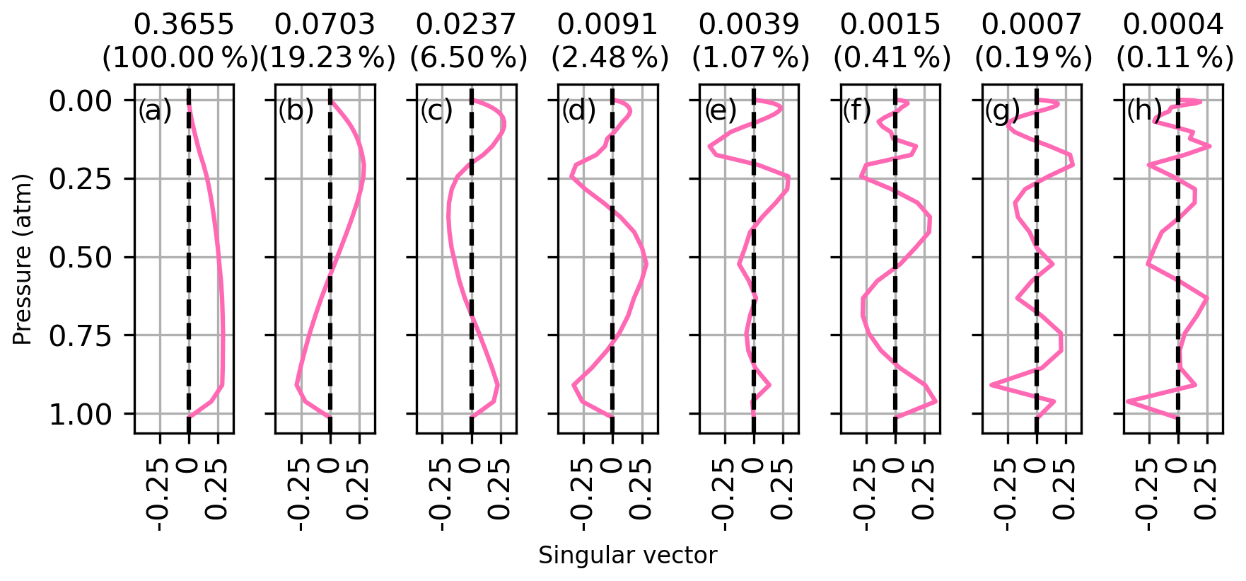
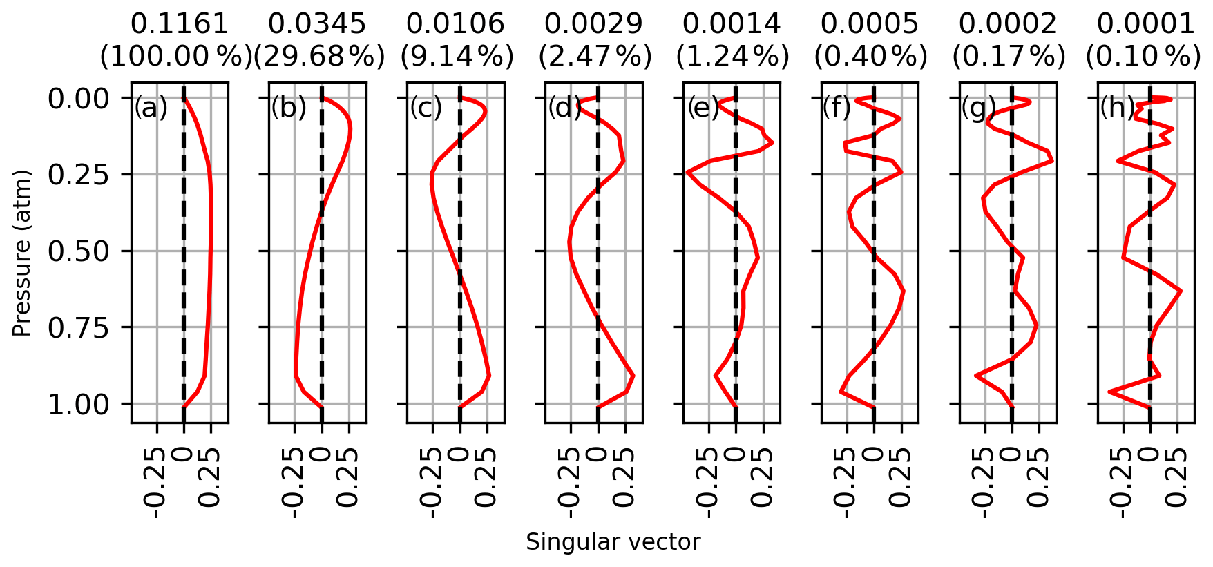
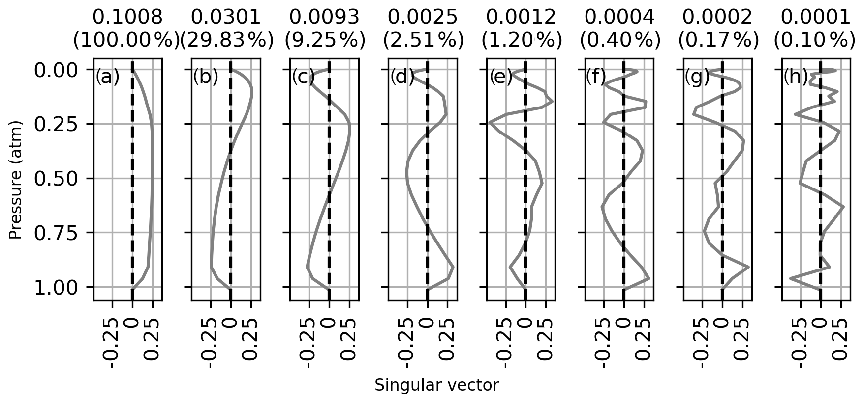
The singular value decomposition of the CO₂ Jacobian matrix can provide information on the relative precision with which different vertical patterns are measured. The Jacobian matrix K is decomposed into

$$\begin{array}{}\text{(D1)}& \begin{array}{rl}\mathbf{K}\left(\mathrm{nmp},\mathrm{nlev}\right)& =\mathbf{U}\left(\mathrm{nmp},\mathrm{nlev}\right)\mathbf{L}\left(\mathrm{nlev},\mathrm{nlev}\right)\\ & \times {\mathbf{V}}^T\left(\mathrm{nlev},\mathrm{nlev}\right),\end{array}\end{array}$$

where nmp is the number of measured spectral points, nlev is the number of atmospheric levels, U is the matrix of left singular vectors, L is the diagonal matrix of singular values, and V^T is the transpose of the matrix of right singular vectors. The right singular vectors of K associated with the eight largest singular values are shown in Figs. D1 to D5 for each CO₂ band on 14 January 2012. The right singular vectors represent independently measured vertical patterns with a precision indicated by their corresponding singular values shown above each panel. The singular values are also shown as a fraction of the largest singular value in parenthesis. The singular vectors all show an increasing number of oscillations with decreasing singular value. In each window, the first singular vector is close to a uniform weighting at all altitudes and has 3 to 10 times more sensitivity than the second pattern. The singular vector in panel (d) has a structure like that of the CO₂ profile deviations observed in the sensitivity tests of Sect. 3.1.

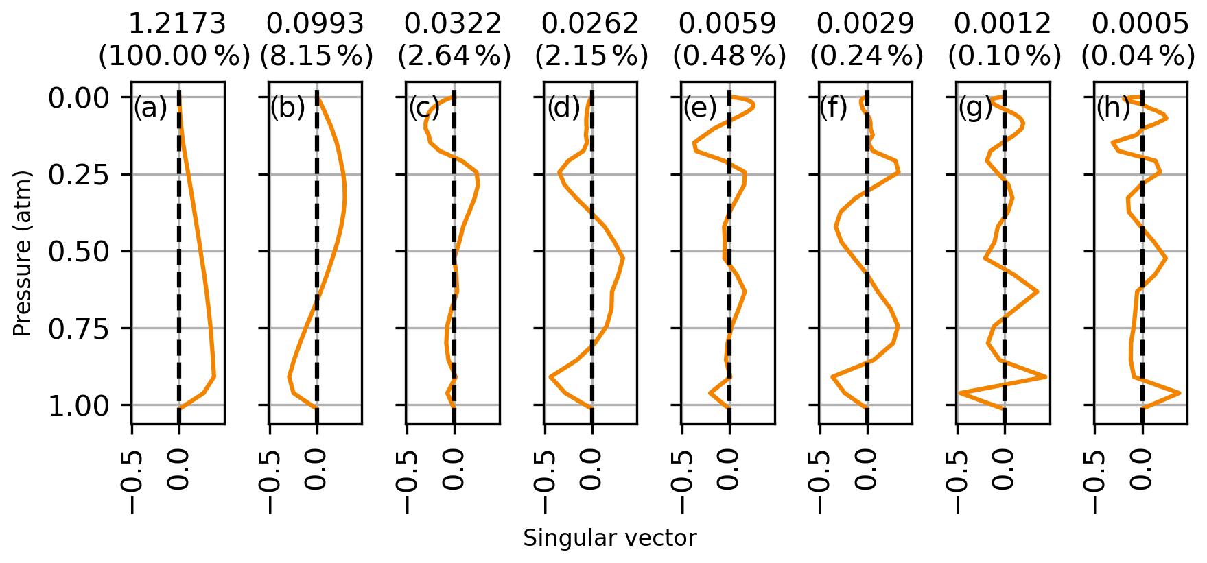
Figure D1 Right singular vector of the Jacobian associated with the eight largest singular values for profile retrievals from the Strong CO₂ window on 14 January 2012. The singular values are shown above each panel, and the singular value normalized to the largest singular value is shown in parenthesis.

Figure D2 Same as Fig. D2 but for the TCCON1 window.

Figure D3 Same as Fig. D1 but for the TCCON2 window.

Figure D4 Same as Fig. D1 but for the Weak1 window.

Figure D5 Same as Fig. D1 but for the Weak2 window.

The retrieval covariance matrix $\widehat{\mathbf{S}}$ can be expressed as a sum of the null space covariance S_N and the measurement noise covariance S_m (Rodgers, 1990):

$$\begin{array}{}\text{(D2)}& {\displaystyle }{\mathbf{S}}_{\mathrm{N}}={\left({\mathbf{S}}_{\mathrm{a}}^{-\mathrm{1}}+{\mathbf{K}}^T{\mathbf{S}}_y^{-\mathrm{1}}\mathbf{K}\right)}^{-\mathrm{1}}{\mathbf{S}}_{\mathrm{a}}^{-\mathrm{1}}{\left({\mathbf{S}}_{\mathrm{a}}^{-\mathrm{1}}+{\mathbf{K}}^T{\mathbf{S}}_y^{-\mathrm{1}}\mathbf{K}\right)}^{-\mathrm{1}},\text{(D3)}& {\displaystyle }\begin{array}{rl}{\mathbf{S}}_{\mathrm{m}}& ={\left({\mathbf{S}}_{\mathrm{a}}^{-\mathrm{1}}+{\mathbf{K}}^T{\mathbf{S}}_y^{-\mathrm{1}}\mathbf{K}\right)}^{-\mathrm{1}}{\mathbf{K}}^T{\mathbf{S}}_y^{-\mathrm{1}}\\ & \times \mathbf{K}{\left({\mathbf{S}}_{\mathrm{a}}^{-\mathrm{1}}+{\mathbf{K}}^T{\mathbf{S}}_y^{-\mathrm{1}}\mathbf{K}\right)}^{-\mathrm{1}}.\end{array}\end{array}$$

The error patterns of these matrices hold information on vertical structures in the CO₂ profiles that the retrieval cannot resolve, due to the smoothing effect of the a priori covariance matrix S_a in the case of S_N, and due to the effect of measurement noise in the case of S_m, as the measurement error covariance matrix S_y only represents random errors in the measured radiances. The error patterns of a matrix are defined as its eigenvectors multiplied by the square root of their corresponding eigenvalue. The error patterns of S_N associated with the four largest eigenvalues are shown in Fig. D6, and those of S_m are shown in Fig. D7. In both cases, the largest error pattern peaks at the surface and falls to 0 at ∼ 0.9 atm; these peaks in the error patterns correspond to a minimum in the singular vectors of the CO₂ Jacobian. The large errors in the retrieved CO₂ profiles are explained by the larger a priori uncertainty in the lower troposphere, and by the relatively larger effect of errors at wavenumbers strongly weighted at low altitudes. This is because “sensitivity” is determined by the Jacobian; the retrieval will simply preferentially adjust CO₂ at levels where a given change in CO₂ causes a larger change in radiance. At pressures larger than ∼ 0.9 atm, the error patterns of S_N represent vertical scales that cannot be resolved in the retrieval, with a vertical scale of 0.3 atm or less.

Figure D6 The four largest error patterns of the null space covariance matrix for a Lamont spectrum measured on 14 January 2012.

Figure D7 Same as Fig. D6 but for the measurement noise covariance matrix.

The uncertainty in the retrieved CO₂ profile is taken to be the square root of the diagonal elements of $\widehat{\mathbf{S}}$ even though the retrieval covariance is not diagonal. It is presented in Fig. D8 as a percentage of the a priori uncertainties. The retrieval error is always smaller than the a priori covariance by construction in optimal estimation, so this alone gives no indication of a successful retrieval. But the retrieval is more sensitive to altitudes where the retrieval uncertainty is a smaller fraction of the a priori uncertainty. The error from the diagonal of S_N and S_m is also shown. In addition to S_N, the smoothing contribution from state vector elements other than CO₂ scale factors is shown as S_i, the interference error covariance (Rodgers and Connor, 2003):

$$\begin{array}{}\text{(D4)}& {\mathbf{S}}_i={\mathbf{A}}_{\mathrm{xe}}{\mathbf{S}}_{\mathrm{a},\mathrm{e}}{\mathbf{A}}_{\mathrm{xe}}^T,\end{array}$$

where S_a,e is the part of the a priori covariance matrix that corresponds to “extra” state vector elements other than CO₂ scale factors. With N total state vector elements and nlev atmospheric levels, S_a,e has dimensions (N-nlev,N-nlev). A_xe is the subset of the averaging kernel matrix that characterizes the smoothing effect of the extra state vector elements on the CO₂ profiles, with dimensions (nlev,N-nlev). The interference error is the smallest contribution to the total error and most of the error comes from the smoothing effect of the a priori CO₂ covariance, followed by the contribution of measurement noise which oscillates between ∼ 10 %–25 % of the a priori CO₂ uncertainty. If temperature were retrieved, for example with a temperature offset or with a scale factor added to the extra state vector elements, we would expect the interference error to increase.

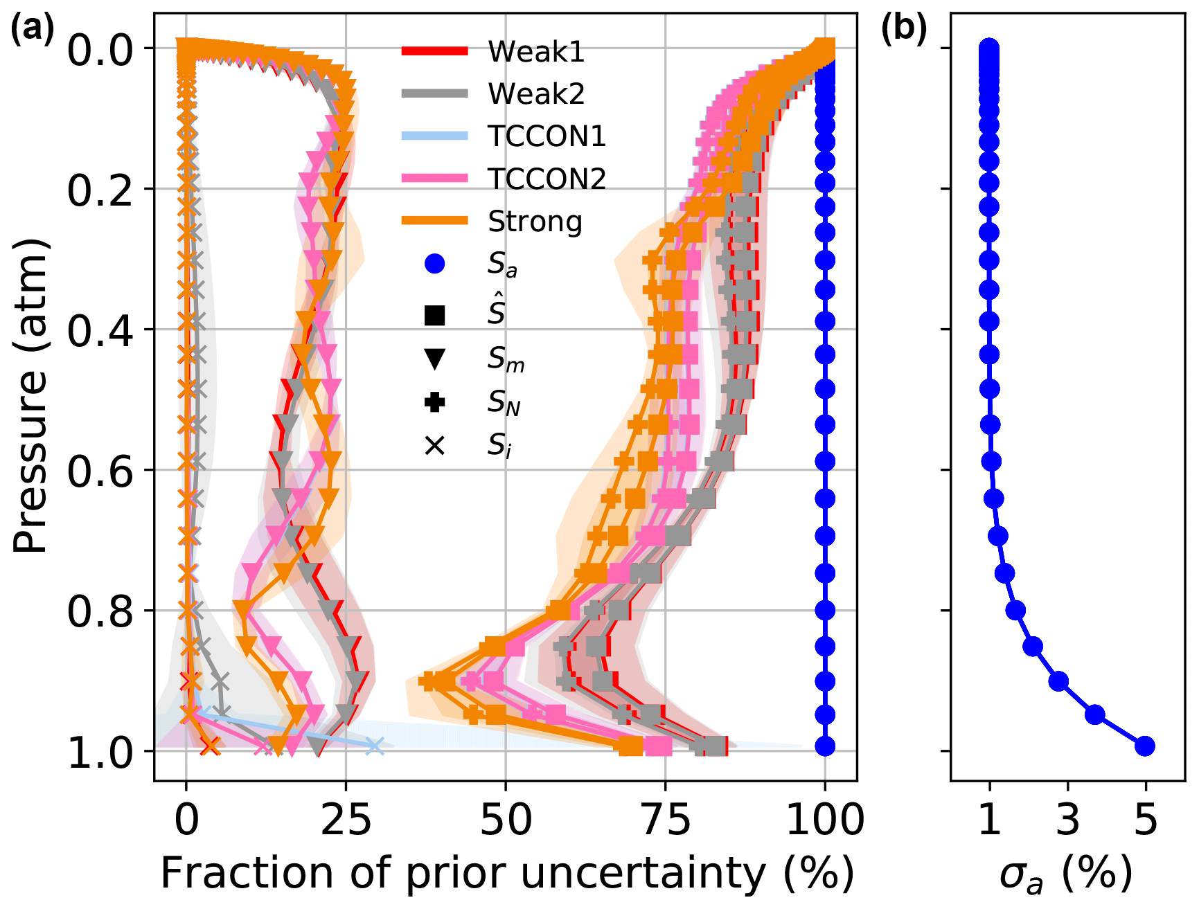
Figure D8 Panel (a) shows the square root of the diagonal elements of the retrieval total error covariance matrix $\widehat{\mathbf{S}}$, the null space covariance matrix S_N, the interference error covariance matrix S_i, and the measurement noise error covariance matrix S_m expressed as a fraction of the a priori uncertainty σ_a. Each line is the average from the set of 8 days with AirCore measurements over Lamont, and the bands indicate the standard deviation. Panel (b) shows the a priori uncertainty.

Appendix E: Empirical corrections

In Sect. 3 we saw that CO₂ profile retrievals have high sensitivity to CO₂ in the absence of errors in the a priori meteorology and systematic errors in instrument line shape. Here we investigate the possibility of empirically removing the effect of those errors by de-weighting systematic spectral fitting residuals using empirical orthogonal functions (EOFs). EOFs have been used, for example, with retrievals from GOSAT and OCO-2 measurements (O'Dell et al., 2018).

E1 Empirical orthogonal functions

To reduce the effect of systematic residuals on retrieved profiles, EOFs of the spectral fitting residuals were derived to find and remove systematic patterns in the residuals related to temperature errors, instrument line shape, and other effects. The residuals divided by air mass from a set of retrievals covering a wide range of observational conditions are stored in a matrix M(m,n), with n the number of spectra and m the number of spectral points. Then a singular value decomposition is performed on this matrix. The columns of the matrix of left singular vectors are orthogonal basis vectors of the residuals and those associated with the largest singular values represent the main patterns in the residuals, while the corresponding right singular vectors can provide information on the temporal frequency of these patterns.

We use a linear combination of left singular vectors. Each singular vector is associated with a scaling factor. The scaling factor is part of the state vector and adjusted during the retrieval using 100 % uncertainty. Before each inversion step, the spectrum “c” calculated with the forward model becomes:

$$\begin{array}{}\text{(E1)}& c=c+\sum _{i=\mathrm{1}}^N{a}_i{u}_i,\end{array}$$

where N is the number of EOFs to use, ordered with decreasing singular value. The first EOF, associated with the highest singular value, is like the scaled average residual from all the spectral residuals in the matrix M. Our implementation differs from that described by O'Dell et al. (2018) in that here the EOFs are derived from a set of residuals obtained using scaling retrievals, and not using profile retrievals. Since they are meant to remove systematic errors in the calculated spectra before the retrieval adjusts the CO₂ scaling factors, the EOFs should be derived from a large set of residuals obtained with scaling retrievals to have a significant effect on the profile retrieval. If they are derived from residuals obtained with profile retrievals, these mainly include systematic error patterns corresponding to interfering species, which are not the main source of deviations in retrieved CO₂ profiles. When using scaling retrieval residuals, each EOF includes different error patterns corresponding to CO₂ absorption lines. These error patterns may be attributed to systematic errors for the first EOF, such as errors in spectroscopy, or in the instrument line shape, or a persistent bias in meteorology. The error patterns can also correspond to errors in the a priori meteorology. The temporal frequency of each error pattern is contained in the corresponding right singular vector. The right singular vectors could help diagnose, for example, biases in a priori temperature profiles on different timescales. The right singular vectors can also be used to find correlations between each spectral residual pattern and other quantities measured in time, such as differences between a priori and measured meteorology.

If the residual patterns corresponding to CO₂ lines have the same shape as residuals caused by errors in the a priori CO₂ profile shape, adjustments to the CO₂ scaling factors will compete with adjustments to the EOF scaling factors in the retrieval. Because higher-order EOFs are associated with residuals with different time periodicity, they can also introduce errors that do not exist in calculated spectra. We chose to only include the first EOF, which represents residual patterns common to most spectra. The leading EOF can explain 40 % to 52 % of the variability in the residuals, depending on the window, as shown in Fig. E1. The fraction of variability is obtained as the singular value of a given EOF divided by the sum of all singular values. The first 10 EOFs in each window are above the noise level of singular values and account for over 90 % of the variability in the residuals.

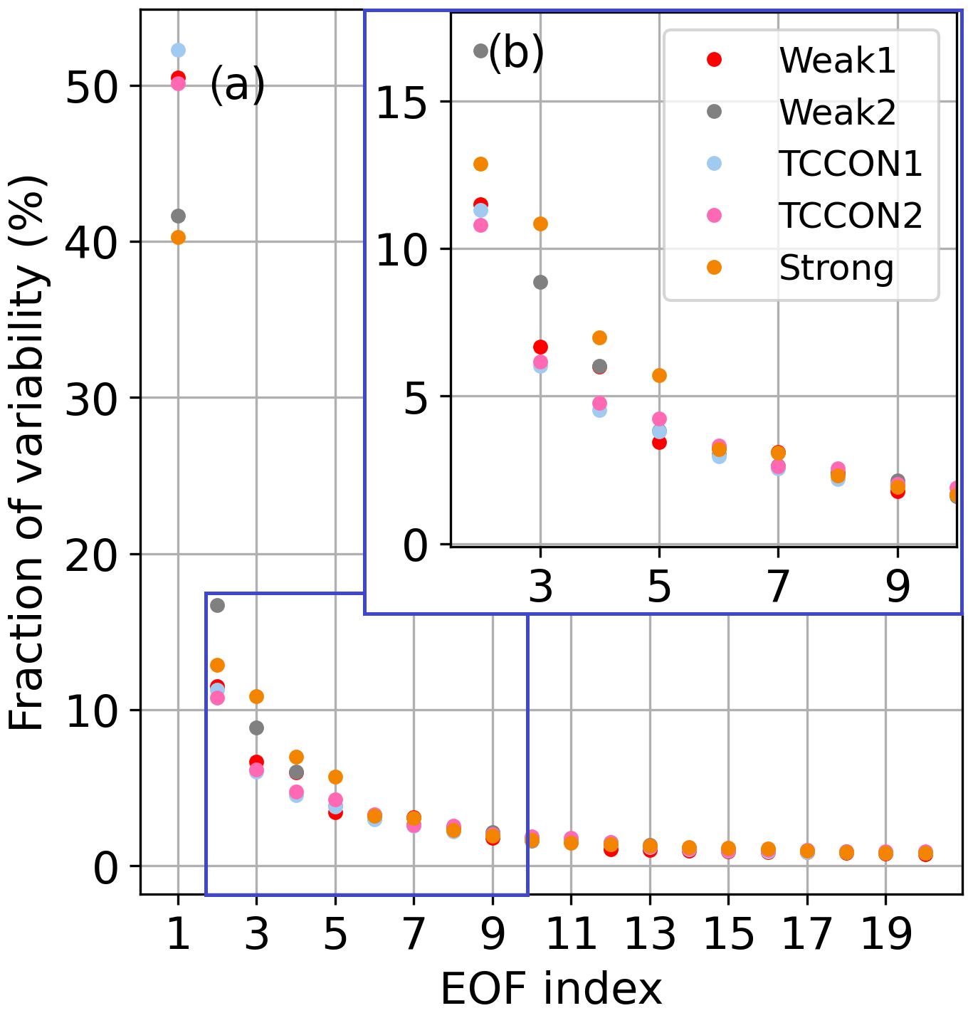
Figure E1 Fraction of the variability in the spectral residuals accounted for by each empirical orthogonal function in each CO₂ window. The EOF numbers are shown in decreasing order of singular value. Panel (b) highlights the blue rectangle inside panel (a).

E2 Results

One year of measurements from the East Trout Lake (SK, Canada) TCCON station were processed in three ways: with scaling retrievals, with profile retrievals, and with profile retrievals including the first EOF derived from residuals obtained with the scaling retrievals. The residuals used to derive the EOFs are filtered such that spectra that would not pass the TCCON quality checks are not included. To avoid isolated spectra with large residuals having a disproportionate impact on the singular value decomposition of the matrix of residuals, all the spectra are ordered by increasing solar zenith angle and filtered based on the root mean square of the residuals: the 500-point rolling median is computed, and the median of the 500-point rolling standard deviation is used as an estimate of the standard deviation σ; then only spectra within 1σ of the rolling median for all windows are used to derive the EOFs. The matrix of residuals resulting from this filtering includes 42 037 out of 64 245 total spectra. XCO₂ was retrieved from each window separately. The statistics on the retrieved XCO₂ error are shown in Table E1 for each retrieval type and for each window. In all windows but the Strong window, the changes in XCO₂ error between the different retrieval methods are small, less than 0.05 ppm. This is 8 times smaller than the reported TCCON 1σ single-measurement precision of 0.4 ppm. However, the mean XCO₂ error is ∼ 55 % larger in the strong window with profile retrievals compared to scaling retrievals.

Table E1 Statistics on the retrieved XCO₂ error for one year of measurements at the East Trout Lake TCCON station. “SD” indicates the standard deviation.

Figures E2 to E6 show quantities derived from each type of retrieval for an example day and for each window. In each window, the profile retrieval with the first EOF appears as an intermediate case between the profile retrieval and the scaling retrieval. In each case, the root mean square of the residuals is smaller for profile retrieval with the first EOF, but the XCO₂ error is not necessarily smaller.

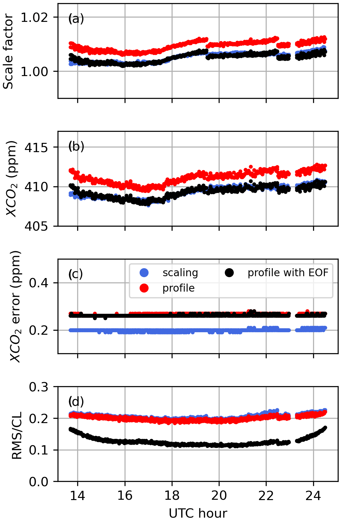
Figure E2 Quantities derived from retrievals on East Trout Lake measurements on 29 March 2018 for the Strong window. The retrieval type is indicated by the legend. Panel (a) shows the column-integrated CO₂ scale factor. Panel (b) shows XCO₂ and panel (c) shows the XCO₂ error. Panel (d) shows the root mean square of the residuals as a fraction of the continuum level.

Figure E3 Same as Fig. E2 but for the TCCON1 window.

Figure E4 Same as Fig. E2 but for the TCCON2 window.

Figure E5 Same as Fig. E2 but for the Weak1 window.

Figure E6 Same as Fig. E2 but for the Weak2 window.

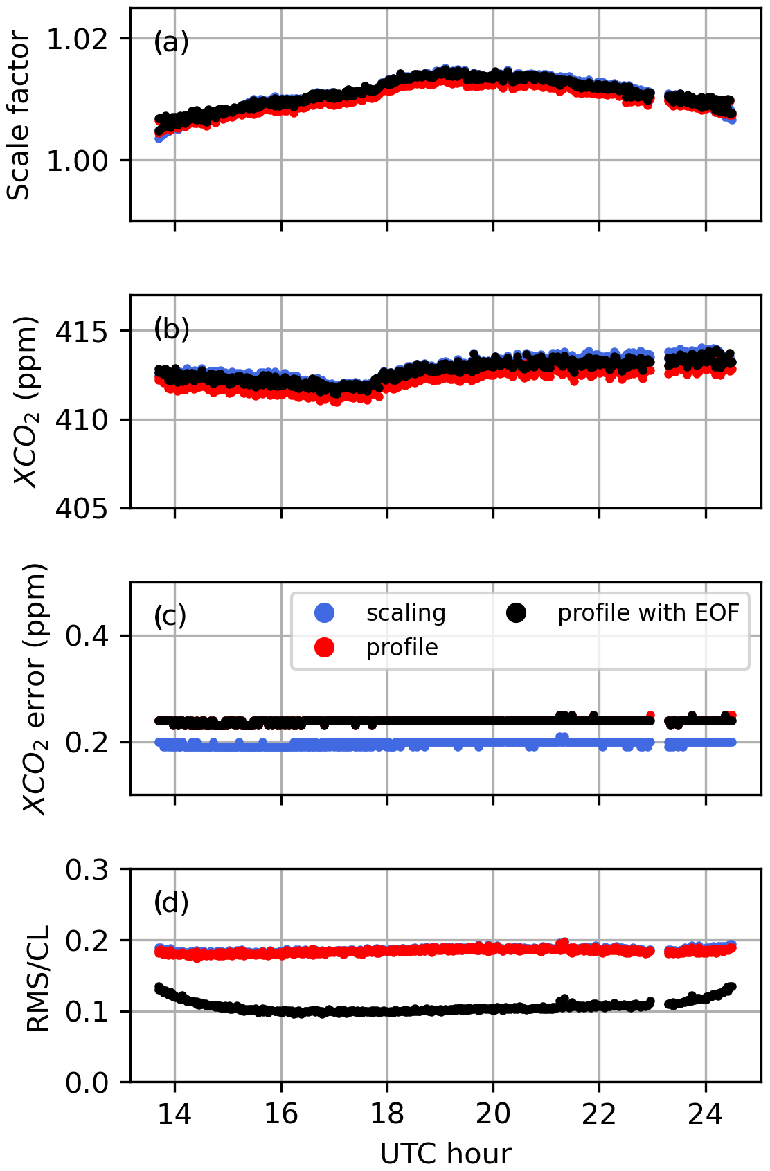
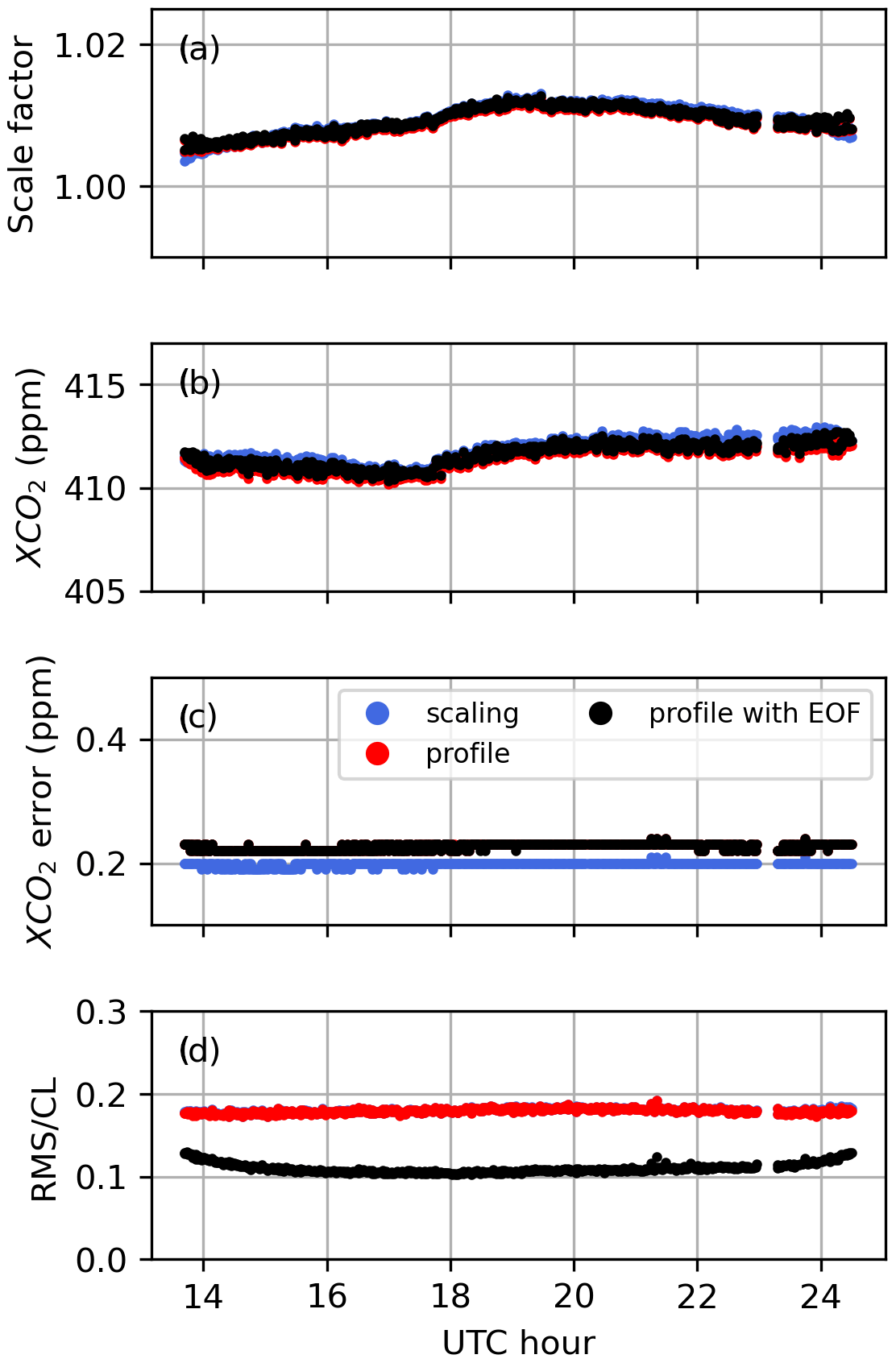
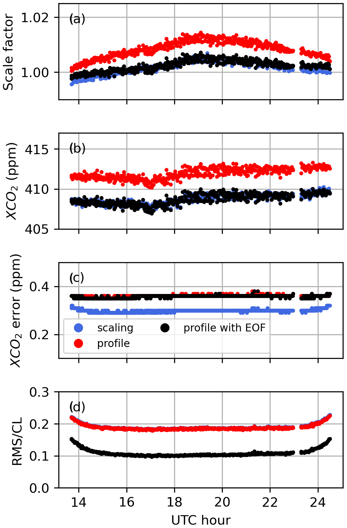
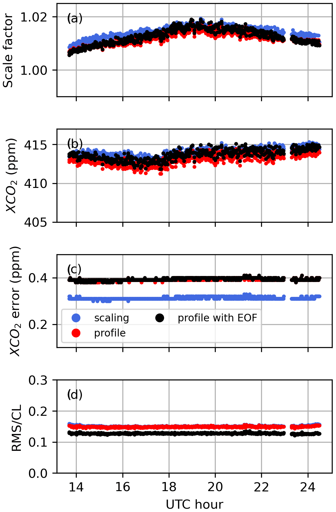
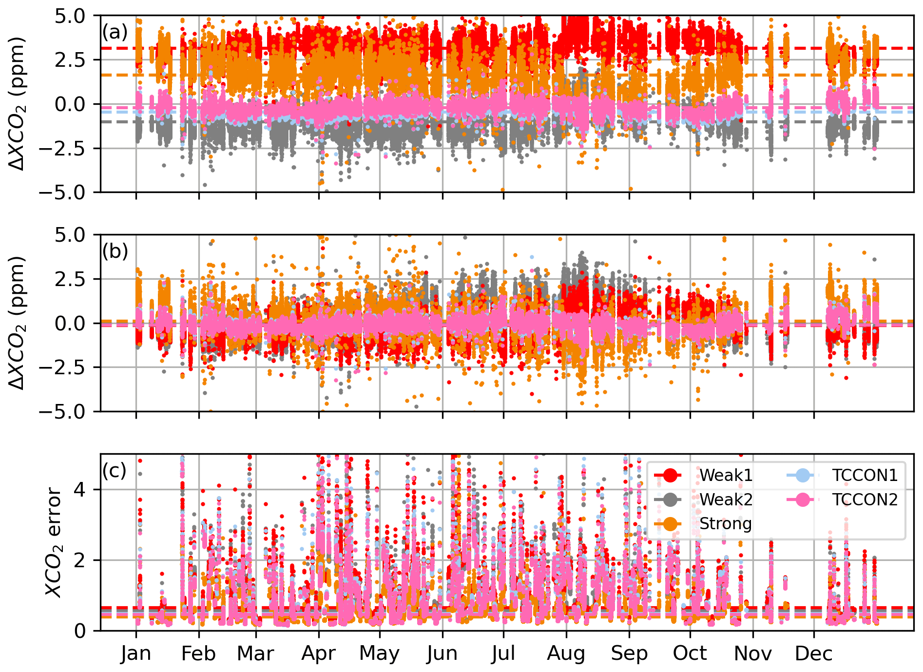
Figure E7 In panel (a), the XCO₂ obtained from the scaling retrieval is subtracted from the XCO₂ obtained from the profile retrieval. In panel (b), the XCO₂ obtained from the scaling retrieval is subtracted from the XCO₂ obtained from the profile retrieval with EOF. In panel (c), the XCO₂ error from the scaling retrieval is shown, with the median values as dashed lines. In the top two panels, the horizontal dashed lines show the median values of absolute differences in XCO₂.

In Fig. E7a, XCO₂ differences are shown between profile and scaling retrievals, and between profile retrievals including the first EOF and scaling retrievals in Fig. E7b. We have seen that differences in XCO₂ error between the different retrieval types are within 0.05 ppm. However, differences in XCO₂ between profile and scaling retrievals can be several times larger than the XCO₂ error, indicating different sources of bias between profile and scaling retrievals. In the Weak1 window, the median of the XCO₂ absolute differences are ∼ 4 times larger than the median XCO₂ error and ∼ 3 times larger in the Strong window. In the TCCON1, TCCON2, and Weak2 windows, the median of the XCO₂ absolute difference is smaller than the median XCO₂ error. In all but the Weak1 window, the XCO₂ differences are 25 % to 35 % smaller between August and November than for the rest of the year. In Fig. E7b, the XCO₂ differences between the profile retrievals with EOF and the scaling retrievals are smaller and more consistent between windows than in Fig. E7a. And the median of the XCO₂ absolute differences is smaller than the median XCO₂ error in all windows. Including the leading EOF in a profile retrieval reduces the XCO₂ differences between the scaling and profile retrievals, but the XCO₂ of the profile retrieval with EOF is more strongly correlated with the XCO₂ of the profile retrieval than that of the scaling retrieval as shown in Table E2.

Table E2 Squared Pearson correlation coefficient for XCO₂ between the scaling and profile retrievals (SCL–PRF), and between the profile retrieval with the first EOF and the profile retrieval (EOF–PRF).

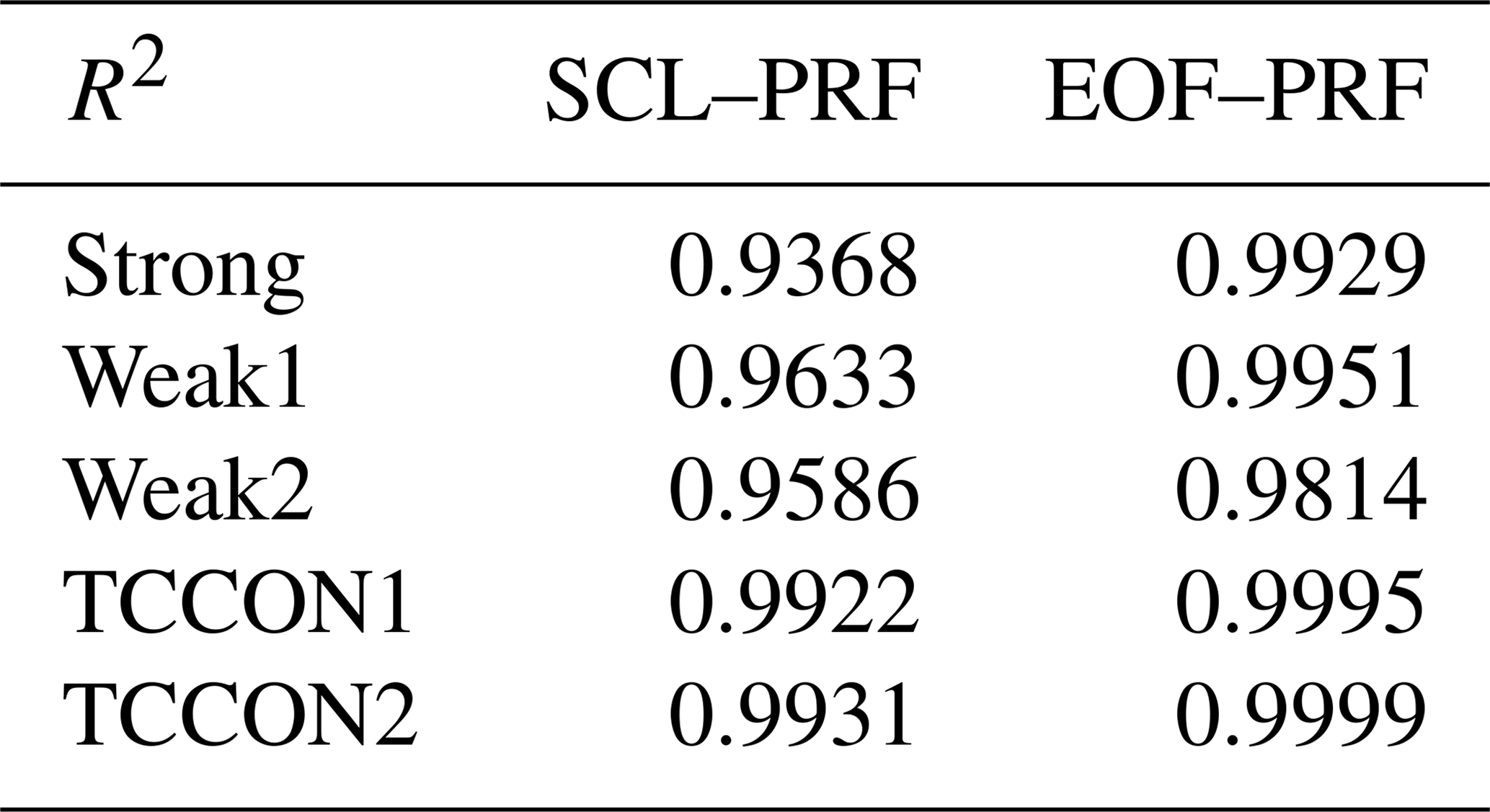
When compared to preliminary data from aircraft measurements, the deviations in the CO₂ profiles obtained with profile retrievals are larger than the vertical variations in the aircraft measurement. When the retrieved profiles present large deviations typical of temperature errors like that in Fig. 9b, the CO₂ profile obtained from profile retrieval with the first EOF reduces the amplitude of the deviations, but the shape persists. This is expected as the first EOF represents the average residuals, which should not include residual features caused by temperature errors, unless the temperature errors were always biased in the same way. We would expect the first EOF to reduce deviations like that in Fig. 9a. In such cases, the CO₂ profiles obtained from profile retrieval with the first EOF are smoother than profile retrievals but present no clear advantage over scaling retrievals.

Appendix F: Synthetic spectra, perturbed field of view and zero-level offset

The saturated lines of the Strong window allow a zero-level offset to be fit. Figure F1 shows the zero-level offset retrieved from the Strong window using real spectra for each of the days with Lamont data used in Sect. 3. The median absolute value is at most 0.001 on 23 July 2013. The effect of a zero-level offset on retrieved profiles was tested with synthetic spectra. Figure F2a and b are the same as Fig. 4a and b and show profiles retrieved from synthetic spectra in the reference case, when no perturbation is applied. Figure F2e and f show the effect of a +0.002 perturbation to the zero-level offset, without retrieving it in the Strong window. This has a large effect in the profile retrieved from the Strong window, with deviations from the truth within 30 ppm, and a smaller effect in the other bands with deviations up to 10 ppm.

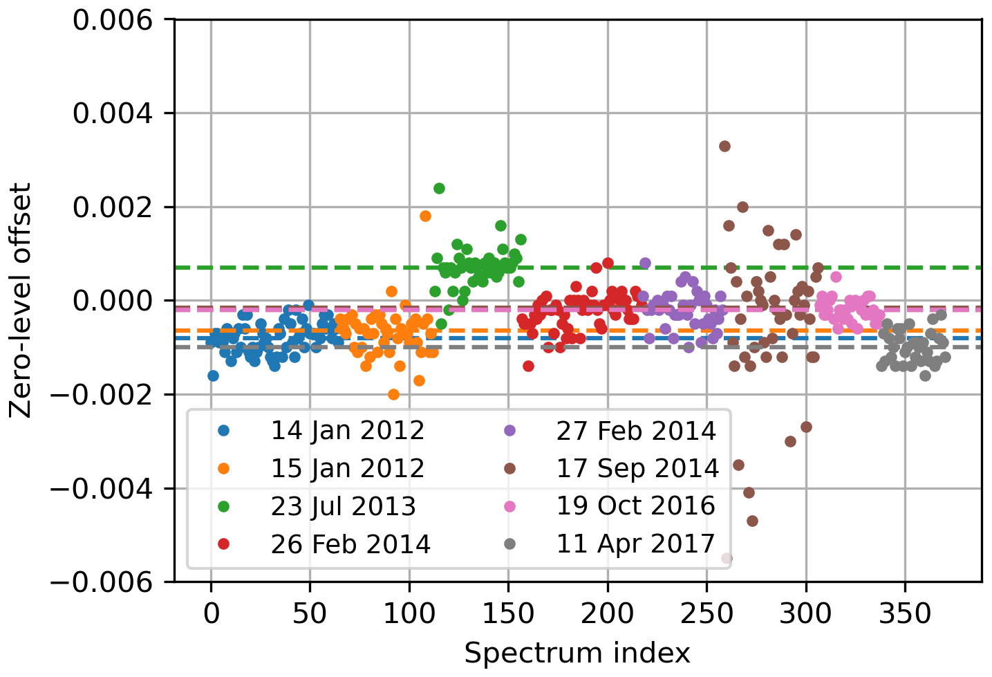
Figure F1 Zero-level offset retrieved from the Strong CO₂ window for the Lamont spectra coincident within ±1 h of the last AirCore sampling time and within ±1.5 h of the closest a priori time on each of the days indicated by the legend. The dashed lines mark the median value for each date.

In Fig. F2c and d we also consider the effect of one type of ILS error by perturbing the internal field of view by +7 %, which leads to a widening of the ILS. The unperturbed internal field of view of the spectrometer is 2.4 mrad. The deviations from the truth are within 1 ppm for P > 0.5 atm and within 3 ppm for P < 0.5 atm.

This sensitivity test shows the effect of zero-level offsets will not be a major source of variability in the retrieved profiles. If the zero-level offset retrieved from the Strong window is added to the TCCON and Weak windows before the retrieval, the change in the retrieved profiles is less than 3 ppm at all altitudes as shown in Fig. F3 using days with AirCore profiles at Lamont.

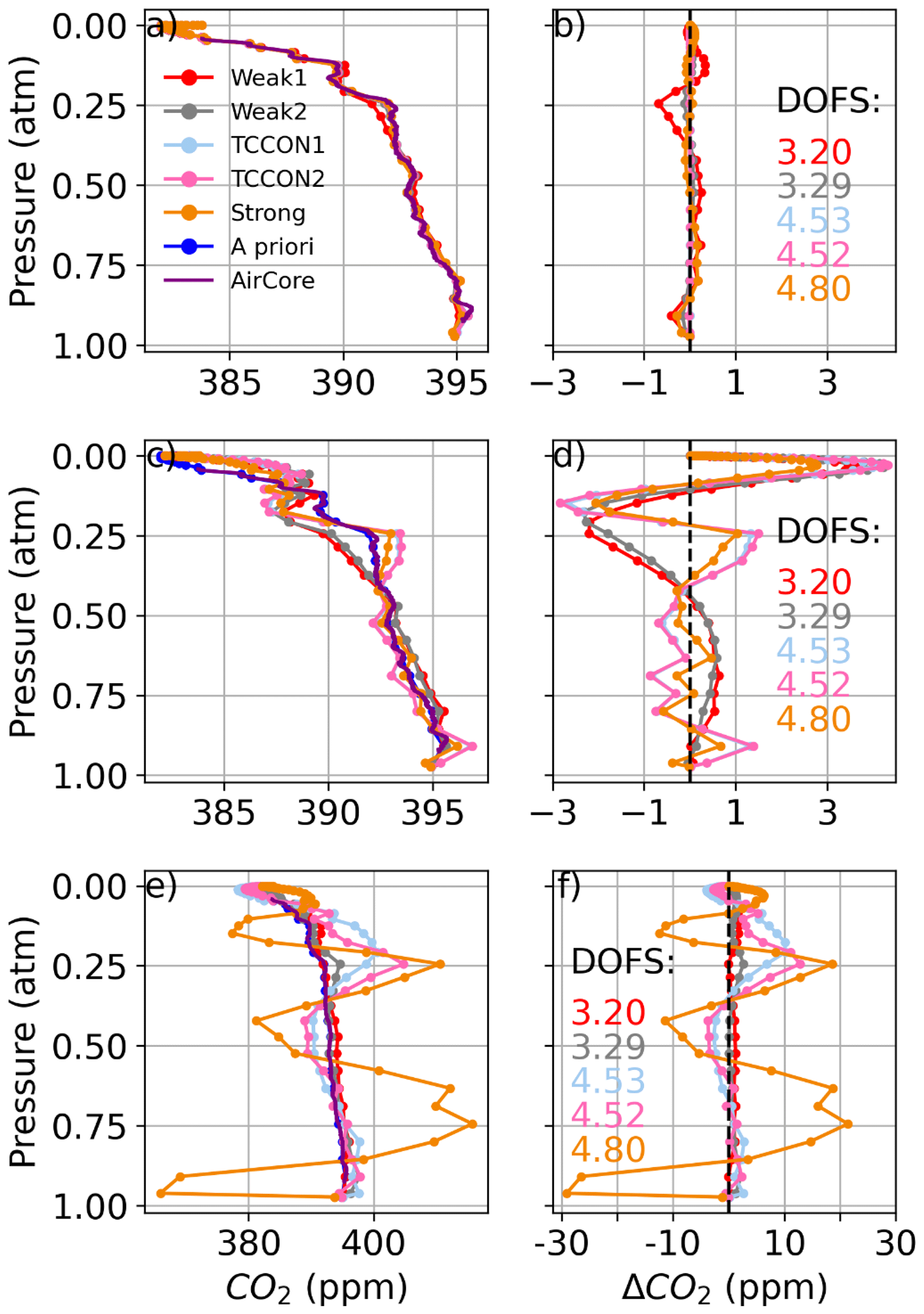
Figure F2 The left-hand panels show CO₂ profiles retrieved using synthetic spectra. In (a), we use the AirCore profile, which was used to generate the synthetic spectra, as the a priori profile. In (c), the internal field of view is perturbed by +7 %, increasing the width of the ILS. In (e), the zero-level offset is perturbed by +0.002 and is not retrieved in the Strong window. Panels (b), (d), and (f) show the difference between the retrieved profiles and AirCore, corresponding to (a), (c), and (e) respectively.

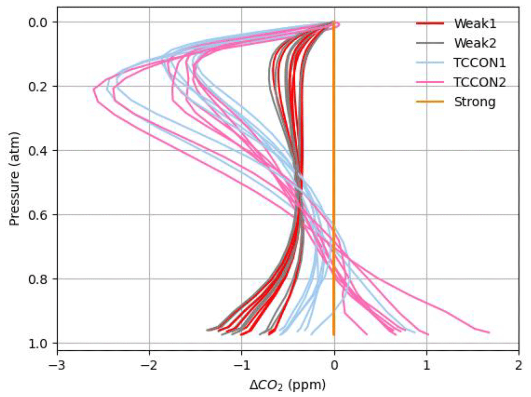
Figure F3 Using real Lamont spectra with the AirCore profile as the a priori profile, the zero-level offset was first retrieved from the Strong window and then added in the Weak and TCCON windows. The difference in the retrieved profiles with and without the added offset is shown for each window and for all the days with AirCore profiles over Lamont. In the Strong window, where the offset is retrieved, the differences are less than 0.001 ppm.