the Creative Commons Attribution 4.0 License.
the Creative Commons Attribution 4.0 License.
 | 29 Apr 2021
RainForest: a random forest algorithm for quantitative precipitation estimation over Switzerland
Daniel Wolfensberger
Marco Gabella
Marco Boscacci
Urs Germann
Quantitative precipitation estimation (QPE) is a difficult task, particularly in complex topography, and requires the adjustment of empirical relations between radar observables and precipitation quantities, as well as methods to transform observations aloft to estimations at the ground level. In this work, we tackle this classical problem with a new twist, by training a random forest (RF) regression to learn a QPE model directly from a large database comprising 4 years of combined gauge and polarimetric radar observations. This algorithm is carefully fine-tuned by optimizing its hyperparameters and then compared with MeteoSwiss' current operational non-polarimetric QPE method. The evaluation shows that the RF algorithm is able to significantly reduce the error and the bias of the predicted precipitation intensities, especially for large and solid or mixed precipitation. In weak precipitation, however, and despite a posteriori bias correction, the RF method has a tendency to overestimate. The trained RF is then adapted to run in a quasi-operational setup providing 5 min QPE estimates on a Cartesian grid, using a simple temporal disaggregation scheme. A series of six case studies reveal that the RF method creates realistic precipitation fields, with no visible radar artifacts, that appear less smooth than the original non-polarimetric QPE and offers an improved performance for five out of six events.
- Article
(14374 KB) - Full-text XML
- BibTeX
- EndNote


Quantitative precipitation estimation (QPE) is well known to be difficult in orographically complex regions such as the Alps (Houze, 2012; Gabella et al., 2017) due to intricate interactions between the terrain and the precipitation and to a large amount of precipitation falling in solid phase. Still, providing an accurate estimate in these regions remains particularly important because the large precipitation amounts in these regions provide essential water resources. Additionally, the hydrological damages can be severe in steep terrain (e.g., landslides, debris flows) which requires fast and accurate warning systems. The most direct and accurate observations of precipitation intensities are obtained using networks of calibrated and well-maintained rain gauges at the ground. Though these measurements are used as a reference, they suffer from inaccuracies in strong wind, especially for solid precipitation (Kochendorfer et al., 2017; Buisán et al., 2017), and provide only a very partial sampling of the precipitation system (Kitchen and Blackall, 1992). Hence, especially for flash-flood and debris-flow alerts, as well as hydrological applications at the catchment scale, these measurements need to be complemented with areal measurements, typically provided by weather radars. Unfortunately, radar measurements are particularly prone to errors and uncertainties in mountainous regions due to the partial or total beam blocking by the orography, which restricts the observations to higher altitudes (e.g., Gabella and Perona, 1998; Germann et al., 2006; Anagnostou et al., 2010). In addition, QPE in solid precipitation is also much more difficult due to the vast heterogeneity of solid hydrometeors and the complex relation between radar observables and intensity (Fujiyoshi et al., 1990; Zrnic and Ryzhkov, 1999).
Traditionally, QPE has involved adjusting relations between polarimetric radar observables and precipitation intensities based either on in situ observations by disdrometers (e.g., Joss et al., 1998; Chapon et al., 2008; Tokay et al., 2009) or by matching the resulting precipitation estimates with gauge observations (Mapiam et al., 2014). While the first approach has the advantage of being physics-based, there is no guarantee that the derived relations are still valid at larger scales (Verrier et al., 2013), and as such it often requires additional bias correction with gauges as reference (Morin and Gabella, 2007). The second approach has the disadvantage of relying too much on potentially flawed gauge observations and is often based only on a limited number of precipitation events. Though power laws are traditionally used as mathematical models to relate radar observables to precipitation quantities, some efforts have been made to train artificial neural networks (ANNs), which are machine learning models able to represent any mathematical function (Cybenko, 1989). An issue with ANNs however is the difficulty to fine-tune them accurately in the presence of noise, which can lead to overfitting and physically unrealistic outcomes.
Currently MeteoSwiss relies on a two-step process to provide the best possible QPE. The first step is a radar-based real-time QPE, which relies on a unique Z–R relationship to convert radar reflectivity to precipitation aloft. This estimate is then corrected for partial beam shielding and extrapolated to the ground with a dynamical vertical profile of reflectivity (VPR) (Germann et al., 2009). The second step improves this radar-based estimate by merging it with gauge observations, using a geostatic interpolation technique called co-kriging with external drift (Sideris et al., 2014), to provide an hourly QPE estimate which is then disaggregated to a 5 min resolution (Barton et al., 2020). Since the development of the radar-based QPE, the radar network of MeteoSwiss has been updated significantly: it now consists of five dual-polarization, Doppler, C-band radars (Germann et al., 2015). The update to dual-polarization offers great opportunities, and the rich additional information it provides is already used operationally for the classification of hydrometeors from radar measurements (Besic et al., 2016) and the identification of ground clutter. Dual-polarization brings additional information, especially in intense precipitation (Ryzhkov et al., 2005, 2014) and solid precipitation (Ryzhkov and Zrnic, 1998; Bukovčić et al., 2018).
The goal of this work is to derive a new data-driven radar-based QPE algorithm that provides accurate precipitation estimates in Switzerland's complex topography and takes advantage of the large archive of polarimetric radar data collected over the years by MeteoSwiss' operational radar network. The algorithm should be as direct as possible to avoid the use of a posteriori bias corrections and should also provide uncertainty estimates. This algorithm should with time replace the first step of the QPE estimation and provide a better input to the gauge–radar merging, which will hopefully also lead to a better final output.
To reach these ends, a non-parametric model for QPE is developed that does not rely on specific power laws but uses random forest (RF) regression to learn a model directly from the data. Random forests (Breiman, 2001) are an ensemble learning method used for classification or regression. The idea behind RF is to train an ensemble of simple decision trees which individually tend to overfit and perform poorly and to aggregate their individual predictions to get a much better and robust estimate. In case of regression, the aggregation method is simply the average prediction of the individual trees. RF has been applied with success in remote sensing, particularly in the domains of hyperspectral data classification and land cover classification (Belgiu and Drăguţ, 2016).
By feeding it with appropriate input features, the presented QPE RF model is able to natively correct the predictions for bright-band and calibration issues and extrapolate precipitation to the ground level, thus simplifying the overall processing chain. Orellana-Alvear et al. (2019) recently presented promising results with an RF approach in the Andes, although with only a single-polarization X-band radar. However, the alternatives to the RF models that are considered in their work are quite simplistic – Marshall–Palmer Z–R relation (Marshall and Palmer, 1948) and custom-fitted power law – and do not include the typical bright-band and local bias corrections that are present in operational QPE models. In this work we go further by considering the full polarimetric radar and ground station network of Switzerland (five C-band radars and more than 270 ground stations) over the course of 4 years of observations, and we compare the performance of this model with the operational state-of-the-art QPE products processed at MeteoSwiss.
This article is structured in the following way. Section 2 provides an overview of the database that was used to train and evaluate the QPE method, and Sect. 3 introduces the random forest regression and the transformation of input data it requires, as well as the performance metrics that are used throughout this work. At the end of the section, these metrics are used to evaluate the performance of MeteoSwiss' current QPE products. Section 4 details the overall performance and the optimal configuration of the random forest QPE. Section 5 completes the previous section by explaining how the algorithm was adapted to a quasi-operational mode where it provides 2D maps of precipitation every 5 min. The performance of the new QPE algorithm is then assessed on a case study of six precipitation events. Finally Sect. 6 concludes this work and summarizes the main advantages and limitations of the proposed method.
Training a machine learning algorithm requires large amounts of data in a homogeneous format. Even though the present archives of MeteoSwiss contain vast amounts of data covering decades of measurements, these data have different spatial and temporal resolutions (from point measurements to large area numerical weather prediction fields), are sometimes temporally inhomogeneous, and are stored in different file formats. Thus an important effort has been invested in the creation of a homogenized dataset that can be used to train any type of machine learning model with the main objective of precipitation estimation but also allowing for other potential uses (e.g., verification of operational products and correction of bias). Note however that only the data that are explicitly used in the present QPE study will be detailed in this section.
Most MeteoSwiss operational products are estimated over a Cartesian grid of 1 km2 (in the Swiss LV03 coordinate system) at a temporal resolution of 2 to 5 min. For numerical prediction, MeteoSwiss runs the COSMO model which is a mesoscale-limited area model that is operated and developed by several weather services in Europe (e.g., Switzerland, Italy, Germany, Poland, Romania and Russia) (Seifert et al., 2011; Doms et al., 2011; Baldauf et al., 2011; Wolfensberger and Berne, 2018). COSMO analysis runs are available over Switzerland every hour1 on a 3D irregular grid. Polarimetric radar data are available every 5 min on a polar grid. Finally, the synoptic weather station data have a temporal resolution of 10 min. To accommodate these differences, the reference temporal resolution of the database is 10 min, and the reference spatial resolution is 1 km2 for spatial data (Cartesian products and polar radar data). Table 1 summarizes the differences in spatial and temporal support between all different data sources used in this work.
Table 1Native and transformed spatial and temporal resolutions of the products included in the gauge–radar database.
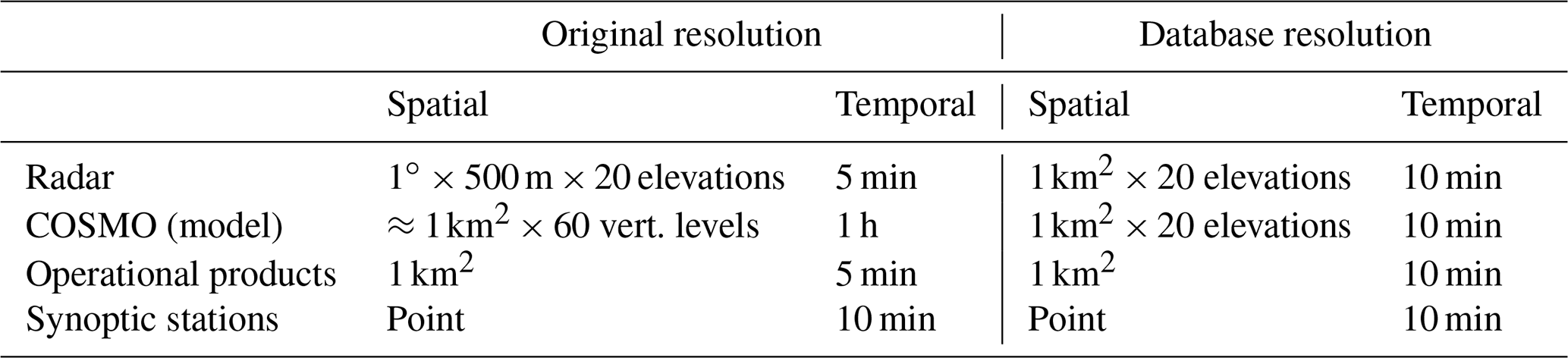
For Cartesian and polar data, the aggregation to 10 min resolution is done by simple averaging. For quantities expressed in decibels such as radar reflectivity, the averaging is done on linear quantities, and the average is converted to decibels. For radar data, three methods for the spatial aggregation to a 1 km2 pixel have been used: mean, in which the average of all observables that fall within a given 1 km2 pixel is taken (with the same consideration as above for decibel quantities); max, in which only data at the polar gate with maximum Zh (within a square kilometer) are taken; and min, in which only the data at the polar gate with minimum Zh (within a square kilometer) are taken. For COSMO data, only the mean aggregation method is used in space, whereas in time a linear interpolation between hourly outputs is made to get to a 10 min temporal resolution.
For radar data and Cartesian products, the extraction is performed separately for a 3×3 pixels neighborhood around the center pixel, in which the synoptic station is located. The data corresponding to the different neighbors are then stored as separate columns in the database.
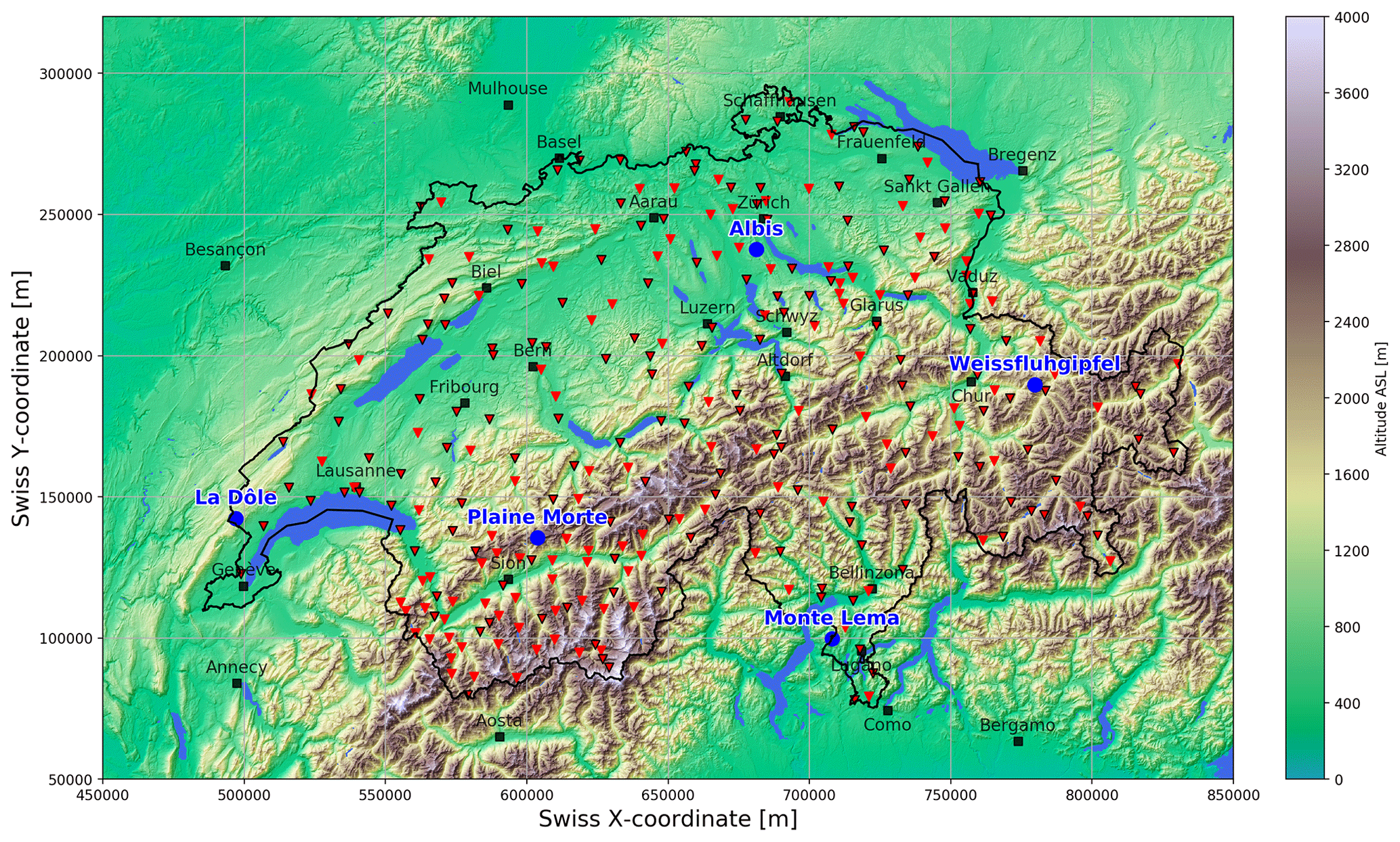
Figure 1Topography of Switzerland with the five Swiss operational radars (blue circles), the 160 synoptic weather stations (red triangles with black border) and the 128 rain gauges (red triangles without borders). Major cities are indicated with black squares. This map is based on a digital elevation model provided by swisstopo.
The database covers 4 years of measurements from January 2016 to December 2019 for the five Swiss radars. To avoid populating the entire database with zeros, at a given station, only the 10 min time steps that fall within an hour when the rain gauge recorded at least 0.1 mm of precipitation2 were included. Note that even if there are no dry hours in the database, at the 10 min resolution, the proportion of observed zero precipitation intensities is still 30 %. The database consists of around 3.3 million observations at the ground, every row corresponding to a different combination of a 10 min time step and station; and there are 18 million radar observations aloft (for the station pixel only, the number of observations for neighbor pixels is similar). Aggregated to hourly resolution this represents a total of around 550 000 station hours at the ground (hourly observation at a given station).
2.1 Synoptic weather station data
Synoptic weather data come from the SwissMetNet (SMN; Suter et al., 2006) observation network which regroups more than 288 stations from which 160 are synoptic weather stations and 128 are rain gauges which only record the precipitated amounts. Note that the area of Switzerland is around 41 000 km2, and the average distance between two stations is 11 km. These stations provide observations every 10 min. Two station observations were used in this study: the precipitation amount over 10 min measured at a height of 1.5 m and the temperature at a height of 2 m. In some stations, precipitation measurements are performed with a tipping bucket Lambrecht rain gauge (types 1518 H3 and 15188), but in most stations an Ott Pluvio2 weighing rain gauge is used instead. All rain gauges are heated to melt solid precipitation but are not shielded from the wind. Temperature measurements are performed with a meteolabor Thygan instrument.
Figure 2 shows the distribution of hourly precipitation observations for the entire database. It can be clearly seen that the distribution is strongly right-skewed, with a vast majority of small intensities and very few but intense extremes. Note that roughly half of the ground observations in the database come from weather stations and the other half from rain gauges, for which no information about air temperature is available. From the weather station observations, only 16 % correspond to temperatures below 0 ∘C.

Figure 2Distribution and statistical indicators of hourly observed precipitation intensities for the entire database (January 2016 to December 2019). The three vertical dashed red bars indicate the percentiles 99, 99.9 and 99.99.
2.2 Radar and COSMO data
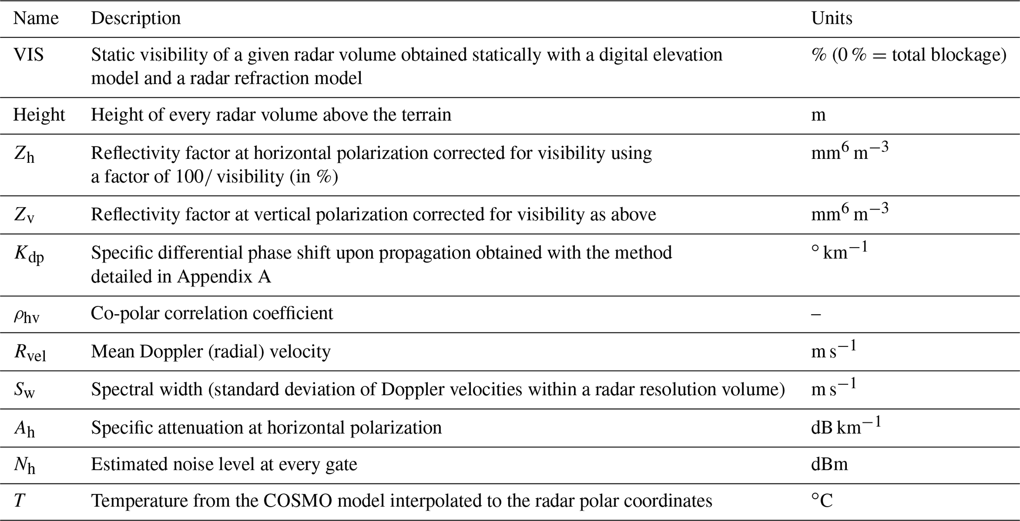
The Swiss radar network consists of five polarimetric C-band radars which perform plan position indicator (PPI) scans at 20 different elevation angles3 (Germann et al., 2006) using an interleaved scanning strategy. The polar data used in this study consist of the final quality-checked measurements corrected for ground clutter and calibration and aggregated to a radial resolution of 500 m (over six consecutive range gates). In addition to radar observations, the temperature from the COSMO numerical weather prediction model has been interpolated to the radar grid using nearest-neighbor interpolation. The radar and COSMO variables that have been used in this study are listed in Table 2.
Table 2List of radar and COSMO variables used aloft the synoptic stations.
2.3 MeteoSwiss Cartesian reference products
Two types of MeteoSwiss Cartesian products have been used in this study.
2.3.1 RZC
RZC is the standard operational purely radar QPE product of MeteoSwiss (Germann et al., 2006; Gabella et al., 2017). It provides 2D maps of precipitation intensities in millimeter per hour (mm h−1) equivalent liquid water every 5 min. The algorithm starts by estimating the precipitation intensity at every radar gate from the reflectivity with the power law Z=316R1.5 (Joss et al., 1998), where Z is linear reflectivity (in units of mm6 m−3), and R is precipitation intensity (in mm h−1). Prior to this transformation, gates with low visibility VIS (VIS≤37 %) are discarded. The values are corrected for partial beam shielding by applying a multiplicative correction of VIS (in %). To account for growth and decay of precipitation with altitude, a correction with a dynamic vertical profile of reflectivity (Germann and Joss, 2002) is then applied to every R value aloft. Recently, a novel algorithm relying on ANN to extrapolate radar measurements to the ground has been developed at MeteoSwiss by van den Heuvel et al. (2020). This approach gives promising results and often outperforms the classical VPR method. This method is however not yet implemented in the operational workflow. In the current algorithm, the R values aloft are integrated to the ground using a weighted sum, linearly related to the visibility and exponentially related to the height of observations: , where h is the height above ground of the observation in meters. Obviously the negative factor in the exponential implies that observations closer to the ground have a larger weight. These weighted averages are then resampled to the Cartesian 1 km2 grid. Finally a multiplicative local bias correction is applied at every Cartesian pixel to obtain the final R estimated at the ground; see Germann et al. (2006), in particular “Experiment” in Table 2 (p. 1684), Fig. 8 (p. 1686) and Sect. 5.
2.3.2 CPC
CombiPrecip (CPC) is a combined gauge–radar QPE product developed by Sideris et al. (2014). The merging is performed with a geostatic method called co-kriging with external drift, in which the spatial dependence of radar and gauge observations are fitted dynamically with an exponential law. The gauge data are then interpolated in space and time (co-kriging) to the Cartesian grid as a primary variable using the radar data as a trend (drift). This method only yields an hourly estimate, but a recent algorithm by Barton et al. (2020) is used operationally to produce 5 min CPC estimates by disaggregating hourly CPC estimates with hourly fractions of 5 min RZC estimates. Also note that at every gauge in Switzerland an hourly cross-validation product called CPC.CV is computed using a leave-one-out strategy (the gauge for which the CPC performance is assessed is not used in the algorithm).
3.1 Choice of a regression method
Thanks to this large database of collocated gauge and radar observations, a QPE model can be trained and used for the further prediction on new data, providing a 2D Cartesian estimate on the same grid as the current QPE product (Sect. 2.3.1).
To be used in an operational context, the QPE method must be fast (real-time use) and robust in the case of faulty radar measurements, both during training and the subsequent prediction of new values. Obviously, it should benefit from polarimetric information which is not used in the current RZC method. Moreover, unlike the current method it should provide an unbiased estimate that does not require additional local corrections. Three machine learning regression methods were considered: artificial neural networks (ANNs), gradient boosting (GB) and random forests (RFs). The advantage of RF is the simplicity of the hyperparameter tuning and the inherent parallelization of the training and predicting. RFs are not able to extrapolate, meaning that the input dataset has to be representative of all cases that can be encountered in nature. ANNs are powerful and easy to parallelize but require careful tuning and can easily overfit in case of noise, leading to unphysical predictions. GB can be extremely powerful and does not extrapolate but is harder to parallelize and to tune. Preliminary tests showed that without extensive fine-tuning the three methods provide relatively similar performance. Due to its numerous advantages it was thus decided to use only random forest regression.
3.2 Random forest regression
Random forests (Breiman, 2001) are an ensemble learning methodology, in which the outcomes of a number of trained weak learners (in this case decision trees) are combined with a voting scheme to yield a boosted estimate with a better performance. This is inspired by the wisdom of the crowd process, in which a collective heterogeneous group of individuals is better at analyzing and solving a complex problem than single individuals, even if they are experts. To guarantee the heterogeneity of the weak learners, RF includes bootstrap resampling and random feature selection. Let us assume that the input dataset has dimensions of N×M, where N is the number of samples and M the number of input features. For each tree in the forest, a new training set with N samples is created using bootstrap sampling (random selection of samples with replacement). For each training set a new decision tree is grown using the CART method (Breiman et al., 1984). Every time a new split has to be made at a given node of the tree, only a number m of features (m<M, typically ) are randomly selected. This process, which is trivial to parallelize is repeated until t trees are grown, giving a random forest. In the case of random forest regression, the final prediction is simply the average of all outcomes of the individual trees of the forest. The hyperparameters of the random forest regression model which need to be fine-tuned with cross-validation are as follows:
-
the number of trees t in the forest
-
the maximum depth d of the individual trees (i.e., how many times a split is made; trees that are too shallow will be biased too much, whereas trees that are too deep will be overfitted)
-
the number of features m randomly considered when splitting a decision tree
-
the minimum number of samples in a node to split it
-
the minimum number of samples in a leaf (child node) to accept a given split.
Because RF regression uses the average of the tree predictions, they tend to underestimate extreme values and overestimate small values (Zhang and Lu, 2012). Even if it is very rare and does contribute only marginally to the total precipitation amounts, extreme precipitation is a key part of QPE since it causes the largest impact on landscapes, ecosystems and human activities. Consequently, to allow RF to better represent large values, the last two parameters (minimum number of samples in a node and in a leaf for a split) have been set to 2 and 1, which is also the default in the scikit-learn (Pedregosa et al., 2011) machine learning library that was used to train the RF algorithm. This implies that the splitting procedure is not affected by the size of the node and the generated leaves.
Moreover, in order to further mitigate the inherent bias of RF, three types of a posteriori bias correction (BC) methods were compared.
- BC_raw
-
A polynomial regression of predictions versus observations (from gauge) on the training dataset is performed, and this fit is then used to correct new RF predictions.
- BC_cdf
-
A polynomial regression of sorted predictions versus sorted observations on the training dataset is performed, and this fit is then used to correct new RF predictions. This can be seen as a form of histogram matching since it maps the cumulative density function (CDF) of predictions to the CDF of observations.
- BC_cdf_spline
-
Same as BC_cdf but a cubic spline is used instead of a simple linear regression.
Figure 3 shows an example of predicted values versus observations on the training fraction and the first order bias-correction methods that were fitted to the data. Comparisons with the 1:1 line show that high intensities are generally underestimated. The bias-correction methods apply a factor to every new prediction that should bring them closer to the 1:1 line. Note that the relative performance of these BC methods needs to be assessed on an independent test dataset.
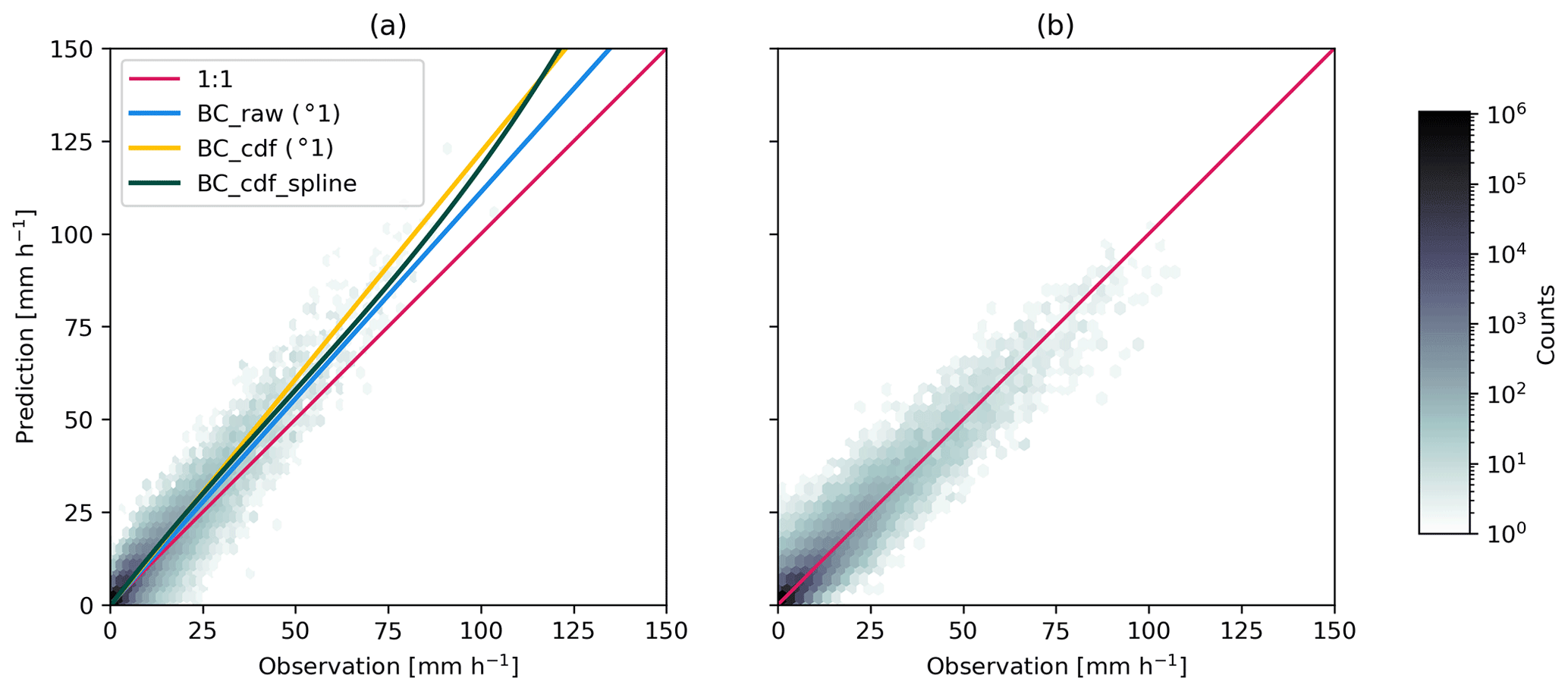
Figure 3Panel (a) shows an example of raw uncorrected predictions (as a density plot) versus observations on the training fraction. The blue, yellow and dark green lines are the corresponding fitted bias-correction models which try to estimate the observed value as a function of raw predicted values. Panel (b) shows the raw predictions corrected with the BC_cdf_spline method (dark green line in panel a), which brings them much closer to the 1:1 line.
3.3 Transformation of radar data
In the database a column of radar observations is available aloft over every station. Reference precipitation observations are however only available at the ground. Machine learning methods require consistent dimensions of input features and response (observations). Therefore, radar data need to be aggregated to the ground level. In our model, taking as an example the current RZC QPE, the radar data are aggregated to the ground using a similar weighted sum:
where the β parameter indicates the slope of this exponential and was fine-tuned with cross-validation alongside the other RF hyperparameters (Sect. 3.2).
This transformation allows us to derive five additional variables: Fracrad_r, which is the fraction of observations aloft that come from radar r (r being one of the five operational radars). This fraction is weighted in the same exponential way, meaning that for a given radar, the presence of observations at low altitudes gives a larger increase in the fraction. Note that since these variables are all related to the others, they will be grouped together under the general term Fracrad.
3.4 Performance metrics
In order to assess the performance of the QPE method and to compare it with the current RZC algorithm, pertinent performance metrics are required. A single metric is usually not sufficient to represent the error structure; hence, in this work we will use four different complementary metrics. Let us use the notation Y for the response variable (observed precipitation intensity) and for the QPE estimation.
- RMSE
-
The root mean square error is in units of millimeters per hour (mm h−1):
where ME is the mean linear error (bias) and STDE the standard deviation of the errors. RMSE, because of the use of an exponent of 2, is quite sensitive to large deviations occurring for high precipitation rate values.
- scatter
-
The weighted interquantile (16 %–84 %) of relative bias is in decibels (dB) (Germann et al., 2006):
where
and Qw is a weighted quantile (Edgeworth, 1888), where the weights w are related to the observed precipitation intensity:
- logBias
-
The relative bias is in decibels (dB):
- ED
-
The energy distance is a unitless measure of the statistical distance between two distributions (Rizzo and Székely, 2016):
The prime symbol indicates the difference between pairs of successive values, and the norm is the standard Euclidean norm.
The two first metrics are estimates of the error of the QPE model: the RMSE is a measure of the additive error and is more sensitive to extreme values, whereas the scatter is a robust measure of the relative error since it ignores the tails of the distribution. The third metric is a measure of the relative bias of the QPE model, expressed in logarithmic scale. The last metric measures the match of the predicted precipitation distribution with the observed values. As such it does not indicate if a single predicted precipitation value is correct but only that the global population of predicted values is representative of what is observed in nature. As in Sideris et al. (2014), Speirs et al. (2017), and Panziera et al. (2017), the performance metrics will be mostly evaluated at hourly resolution (aggregation of six consecutive 10 min time steps) because of the limited representativeness of the gauge data (due mostly to the spatial undersampling of the gauge but also to wind effects and limited accuracy of the instrument). This also avoids numerical issues in the logarithmic scores (logBias and scatter) since all hours in the database are rainy, whereas some 10 min time steps are dry.
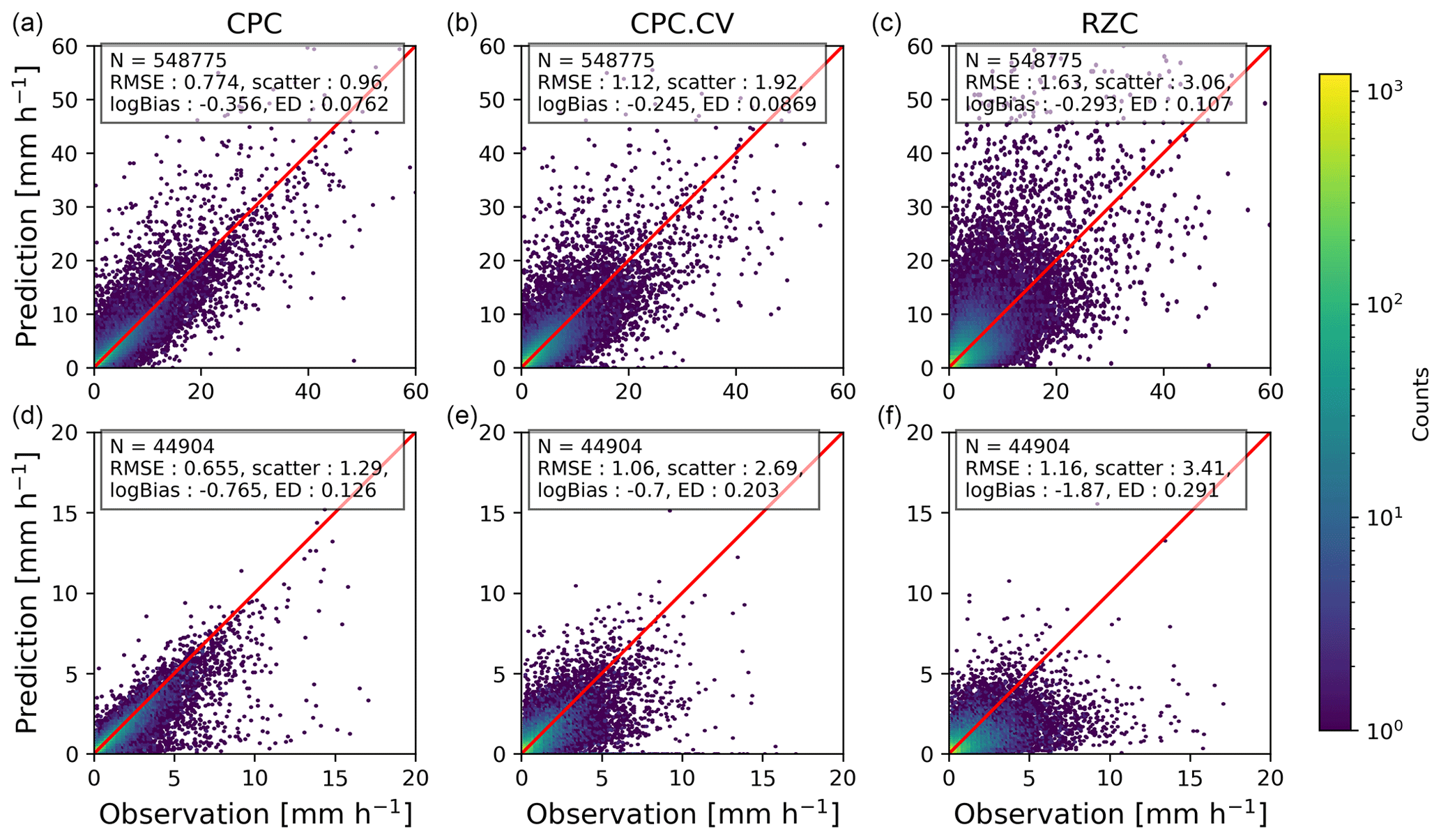
Figure 4Scatter plots and performance scores of the reference products CPC, CPC.CV and RZC for all available observations (a, b, c) and for observations with T<2 ∘C (d, e, f). The 1:1 line is shown in red. The color bar gives the counts in logarithmic scale.
3.5 Performance of reference products
Figure 4 shows the scatter plots of observed precipitation versus reference products (CPC, CPC.CV and RZC) for all observations and for observations with T<2 ∘C, which might correspond to solid or mixed precipitation. Clearly, CPC delivers by far the best performance for all evaluation metrics except logBias which shows the tendency of CPC to underestimate strong precipitation, in particular in snow, a consequence of the smoothing caused by the kriging algorithm. However, since CPC is taking into account the observed gauge measurement, it is not a fair comparison. We will thus restrict the evaluation to the CPC.CV and RZC products. Clearly, RZC has a relatively large overall RMSE, especially for larger intensities; it is however relatively unbiased and has a low ED, indicating that it provides realistic, although sometimes inaccurate, precipitation estimates. It tends however to underestimate quite strongly solid precipitation intensities. CPC.CV provides a systematically better performance than RZC, and the improvement is particularly clear in solid or mixed precipitation. Note that decreasing the temperature threshold from 2 to 0 ∘C decreases the performance on all scores by 10 % to 30 %, but it affects all models in a similar way and as such does not change the general conclusions.
3.6 Filtering of input data
To avoid including spurious data in the training and validation procedure of the random forest, the following data were excluded from the study:
-
Data from the TIT (Titlis), GSB (Grand Saint-Bernard), GRH (Grimsel Hospiz), PIL (Pitatus), SAE (Säntis) and AUB (L'Auberson) stations, where radar agreement has always been poor because of poor radar visibility (very complex topography) and/or suboptimal rain gauge locations (wind-induced undercatching), were excluded. With the exception of the last one (located at 1100 m but with poor radar visibility as it is located in the heart of the Jura mountains), all of these stations are located above 1900 m on mountain summits or passes of the Alps.
-
Data in which Zh aggregated to the ground is larger than 20 dBZ and the gauge measures no precipitation were excluded.
-
Data in which Zh aggregated to the ground is smaller than 5 dBZ and the gauge measures more than 0.5 mm h−1 equivalent were excluded.
The two last constraints reduce the effect of strong advection which leads to a decorrelation between gauge and radar observations due to temporal and spatial shifts of the precipitation field. These three criteria lead to 6.5 % of the data being filtered out (from which fraction condition 1 represents 20 %, condition 2 35 % and condition 3 45 %).
4.1 Choice of input features
To assess the relative importance of all available input variables (Table 2) aggregated to the ground as in Sect. 3.3 and to choose the most pertinent ones, an approach from Han et al. (2016) has been adapted for regression. Assuming as before that M is the number of available input features, the method is described in Algorithm 1.
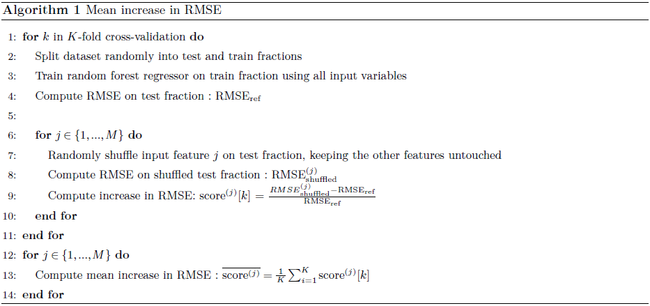
In this study, cross-validation is always done by separating all precipitation events in the dataset and by randomly attributing these events to either the train or test fraction. We define precipitation events as a continuous period of precipitation observations with a time interval of less than 12 h between every observation. In other words, two successive precipitation events are separated by a dry period of at least 12 h in between them. Precipitation events always cover full hours (e.g., from 13:00 to 14:00). This method has the double advantage of increasing the independence between the test and train fractions and avoids including partial hours into the test and train fractions, which is an issue when the evaluation metrics are computed at hourly aggregation. In addition, K in the K-fold cross-validation is always set to 5 (five iterations).
.
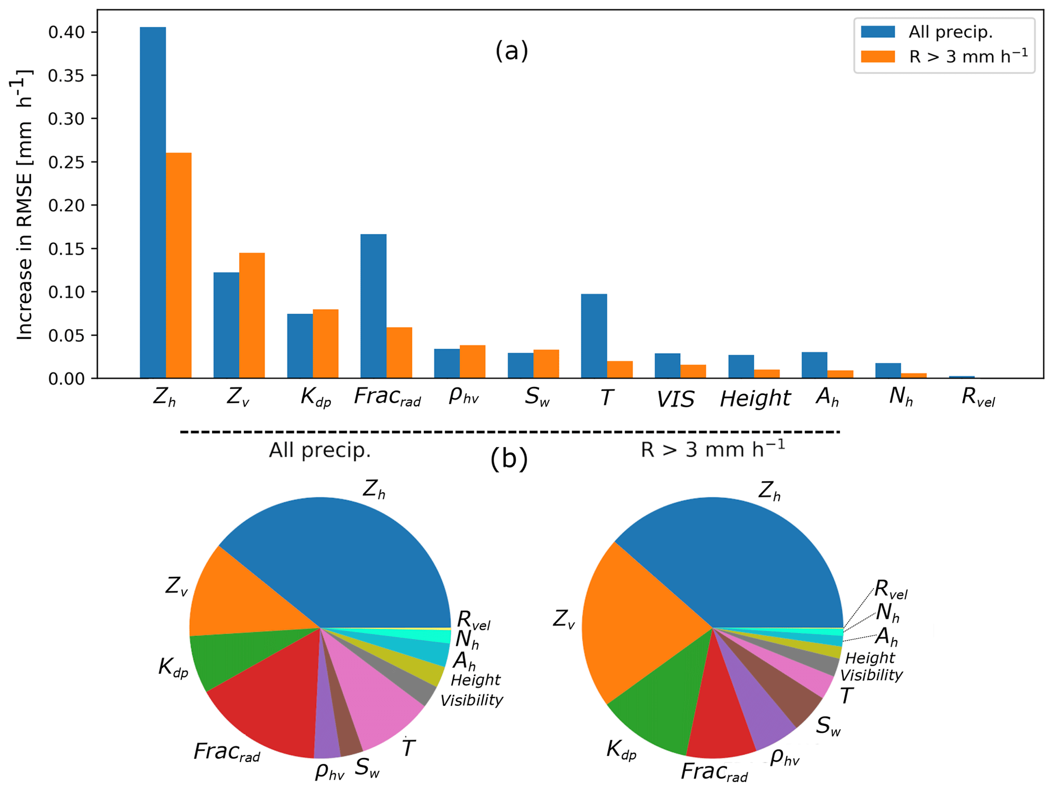
Figure 5(a) Mean decrease in RMSE obtained with Algorithm 1 for all available features, separated for all precipitation and for R>3 mm h−1, and (b) relative importance of these RMSE decreases (normalized by the sum of all decreases). The importance of the feature Fracrad is the sum of the importance of the fraction of every single radar (see Sect. 3.3)
The results of Algorithm 1 are shown in Fig. 5, separately for all observations and for high precipitation intensities. In terms of radar variables, as expected the horizontal reflectivity Zh has by far the highest importance and is followed by the polarimetric variables Zv and Kdp. The fraction of every radar also has a great importance, which can be explained by two factors. First of all the individual radars are not perfectly homogeneous and differ slightly in calibration; this is taken into account in the RZC product by global biases applied separately to all radar observations. Secondly, this is a way for the regressor to account for the spatial precipitation structure over Switzerland; for example, Alpine regions with relatively poor visibility where precipitation tends to be underestimated by the RZC product are characterized by low radar fractions from the three lower radars (Albis, La Dôle and Monte Lema). Surprisingly the spectral width Sw seems to play a relatively large role, which can be due to the fact that it is an indicator of convection (Hooper et al., 2005; Rao et al., 2010), which leads to different relations between precipitation and radar observables. Note also that the relatively low importance of the height (in fact this is the average weighted height of the observations aloft) and the visibility is likely explained by the fact that these variables are already included in the exponential weighting (Sect. 3.3 and, for the visibility, in the correction of Zh and Zv; Table 2). Finally Ah, Nh and Rvel have a low importance on average. For Ah, this is somehow in contradiction to Ryzhkov et al. (2014) who give very promising results for QPE. However, their study was at X-band and requires ray-to-ray fine-tuning of the power-law parameters of the ZPHI method, whereas we used only constant default parameters. There is work in progress to improve the estimation of Ah at MeteoSwiss, but it is a tedious task in complex topography and is thus out of the scope of this work. One should not forget however that even variables with low average importance might in some particular cases be very informative, for example, attenuation in the case of a gauge after a strong thunderstorm.
It is also interesting to notice that for larger intensities, the pie charts in Fig. 5 show a relatively greater importance of Sw (which is an indicator of convection) and of polarimetric variables Zv, Kdp and ρhv and a clear lesser importance of the radar fractions, since discrepancies between radars become weaker for strong signals, and the temperature, since high intensities are mostly related to strong convection, with liquid precipitation at high altitude.
In the final choice of input variables, it was decided to include all 13 features4 displayed in Fig. 5 with the exception of Ah, Nh and Rvel because of their low importance and additional computational cost (for Ah). This model will be referred to as RF_dualpol. For the sake of comparison and to evaluate the possible performance in case of a failure in the vertical polarization channel, one additional model will be tested, RF_hpol, in which only horizontal polarization is available, and ρhv, Kdp and Zv are not included.
4.2 Optimization of hyperparameters
Once the input features have been specified, a grid-search method is used to find the best possible hyperparameters. For every combination of hyperparameters, a five-fold cross-validation is performed in order to get the average performance metrics. The hyperparameters that have been tested are reported in Table 3.
Table 3List of all hyperparameters used in the RF algorithm, as well as the range of values that were tested.

The four performance metrics (Sect. 3.4) were estimated at hourly aggregation for observed precipitation ranges ≤2, 2–10 and ≥10 mm h−1 and for solid precipitation (T≤2 ∘C) and averaged over all cross-validation iterations. The combination of hyperparameters providing the best trade-off between performance for all metrics over all precipitation subsets and computational cost is then found with the following:
where c is a given combination of all hyperparameters . The computational cost is proportional to the number of trees and their maximum depth.
The performance cost is given by
where the suffix z indicates a score standardized over all samples N (z scores):
Note that the weights of RMSE and scatter are halved with respect to the weights of logBias and ED since they are both a measure of error dispersion. The final best trade-off was found with t=15, d=20, m=7, and BC = “BC_cdf_spline”. A comparison of the effect of the choice of hyperparameters on the RMSE, for all precipitation amounts and for high intensities, is shown in Appendix B.
4.3 Stability of the model
A good way to diagnose the completeness of the training data and the stability of a machine learning model is to compute a learning curve (Meek et al., 2002; Praz et al., 2017) that shows the performance on the test and train fractions with increasing number of samples used for training. When looking at this learning curve in Fig. 6, one can conclude that the size of the database seems sufficient to train the model as the test error reaches a plateau for a high number of samples and does not decrease significantly with the number of samples. Note that for random forest regression the train error and its variability tend to be very small since, when considering a large maximum depth of the individual trees (large d), the model is generally able to (almost) perfectly render the response variable on the training set. Because of this, the interpretability of the train error in this case is very limited, and it is hence not displayed.
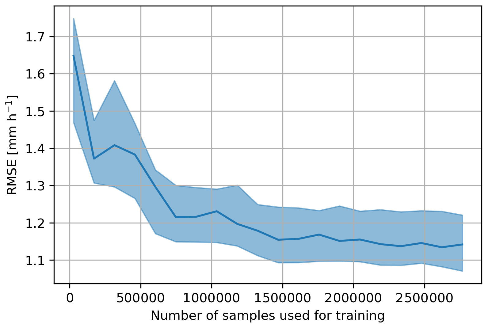
Figure 6Learning curve of the RF_dualpol model. It shows the RMSE of the test fraction at hourly scale as a function of the number of samples used for training. The curve was obtained with 10 iterations of a five-fold cross-validation. The colored areas correspond to the Q25–Q75 interquantile and the solid line to the mean.
Another hypothesis of this QPE model is that the training dataset is consistent through time and there is no major change in the input features that is caused by non-natural phenomena (such as hardware modifications or additional beam shielding caused, for example, by a new construction in the vicinity of a radar). One way to verify this is to look for a trend in the time series of daily cross-validation errors. To this end, the approach of Cleveland et al. (1990) was used to decompose the time series of daily RMSE values into a long-term trend, a seasonal trend and fluctuations that are neither long-term nor seasonal. The results are shown in Fig. 7. It appears that there is indeed no long-term trend in the daily cross-validation error, and besides the obvious seasonal trend (larger intensities in summer), there is no tendency of the model to perform better or worse over some periods of time. As such, if the current radar setup in Switzerland is conserved (as planned), the model should only improve in the future as long as the model gets periodically retrained with an augmented database.
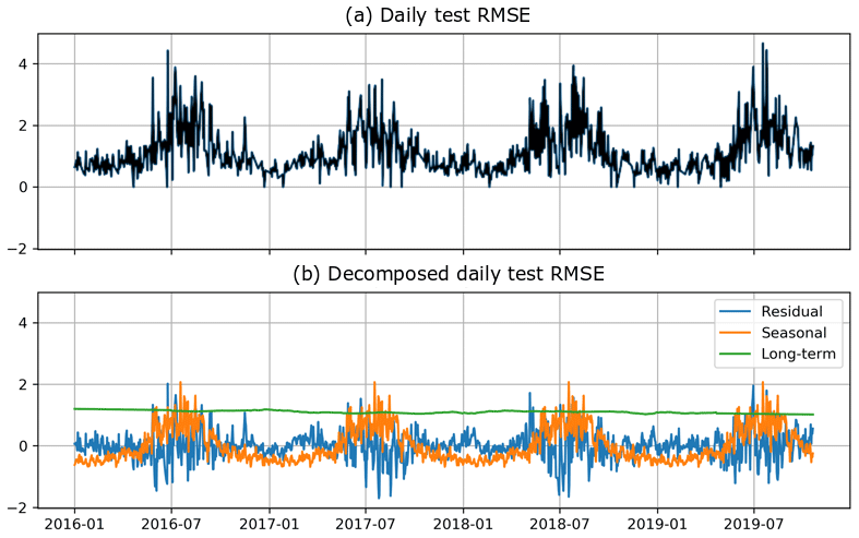
Figure 7(a) Average daily test RMSE obtained from a five-fold cross-validation, (b) daily test RMSE decomposed into seasonal and long-term trends, and fluctuations from these two trends.
4.4 Overall performance of fitted model
The overall performance metrics of the fitted model (averaged over a five-fold cross-validation) at hourly resolution are shown in Fig. 8. It appears clearly that the RF models have a lower error (RMSE and scatter) for both liquid and solid precipitation. However, on average they tend to overestimate liquid precipitation (positive logBias). When looking at different precipitation ranges (see Appendix C); it appears that this overestimation only happens at small precipitation intensities (≤2 mm h−1), which still represent the majority of observations (cf. Fig. 2), and for higher values the RF methods show on the contrary a slight underestimation with respect to RZC (cf. Fig. C1), indicating that the bias correction is not yet perfect. Note also that the RF_hpol model has a consistently poorer performance than the polarimetric model, which could be expected, but still outperforms RZC in terms of RMSE and scatter. Though the RF models do not reach the performance of CPC.CV, they sometimes get quite close and are less biased for certain precipitation ranges. In general RF_dualpol delivers a performance more similar to CPC.CV than RZC.
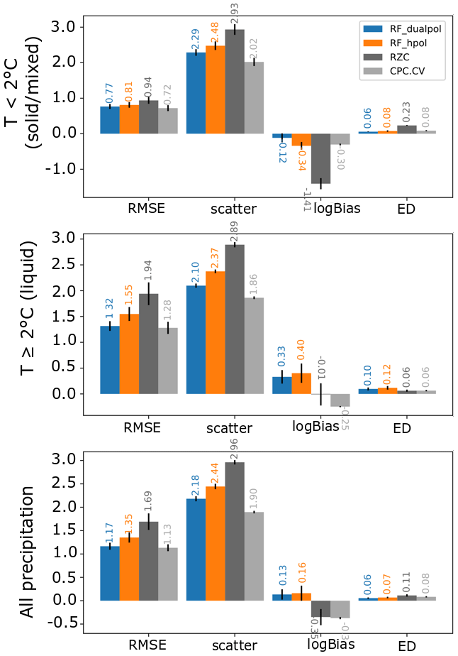
Figure 8Overall performance metrics of the fitted RF models and the references for a five-fold cross-validation. The small black lines at the center of the bars indicate the standard deviation of the metrics over the five-fold cross-validation.
An example of prediction versus observation scatter plots for one iteration of the cross-validation are shown in Fig. 9. It can be seen clearly that for the RF_dualpol method, the spread around the 1:1 line is smaller than for RZC, and there is no visible underestimation trend as can be observed for CPC.CV at higher precipitation intensities.

Figure 9Example of prediction versus observation scatter plots on the test fraction for one cross-validation iteration. The 1:1 line is shown in red.
The performance of the fitted model was also assessed spatially by computing the cross-validation performance metrics separately at every ground station. Figure 10 shows the spatial distribution of the logBias. There is a clear improvement with the random forest methods, with respect to RZC, as areas of strong underestimation in south-central and west-central Switzerland are not visible anymore. The clear overestimation in Valais (southwest) is however still visible. Performance on other metrics (not displayed) show a clear decrease in scatter and to a lesser extent in RMSE and a decrease in the ED of RF_dualpol with respect to RZC, although only in central Switzerland.
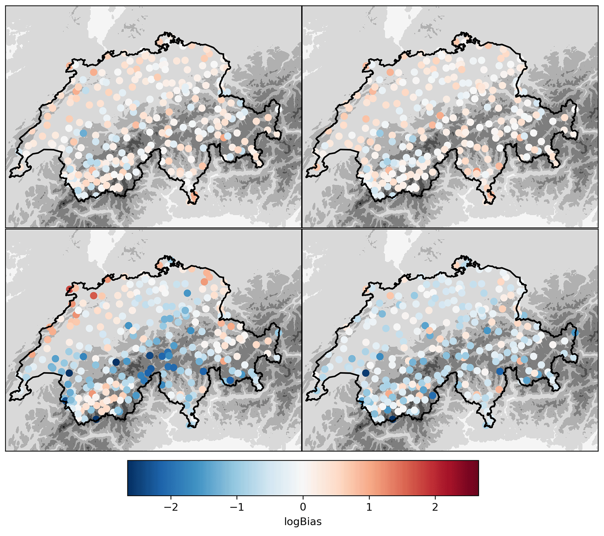
Figure 10Cross-validation logBias at every ground station for RF_dualpol, RF_hpol, RZC and CPC.CV. The displayed geographical domain is the same as in Fig. 1. The gray colors in the background illustrate the topography.
There is generally a trade-off to be found between the bias (accuracy) and the variance (precision) of a model, and underestimating models tend to have a smaller error due to the very asymmetric distribution of precipitation. Figure 11 shows the logBias as a function of the error for all stations. It distinctly shows that RF_dualpol and to a lesser extent RF_hpol are characterized by a better trade-off since the logBias is generally closer to 0 and the scatter is smaller. There is also much less variability between the ground stations, indicating that the model is able to take into account local tendencies.
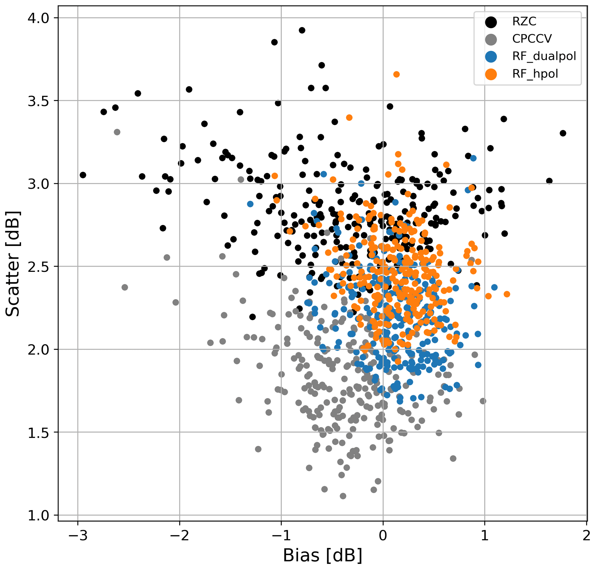
Figure 11Scatter versus logBias at every ground station for RF_dualpol, RF_hpol, RZC and CPC.CV. Every dot corresponds to a different station.
4.5 Error model
Besides a precipitation estimate at every Cartesian pixel, one also needs an estimate of its uncertainty. This uncertainty can be approximated by the error in the cross-validation verification. Figure 12 shows this approximate error as a function of the estimate, as well as possible polynomial fits. It can be seen that the average error tends to be around 50 % of the estimate, and the relative error decreases with increasing prediction. The error of the dualpol model is noticeably lower, which emphasizes again the valuable information brought by the polarimetric variables. Though these average errors seem very large, they are in fact smaller than the one of RZC, which is shown as a black line.
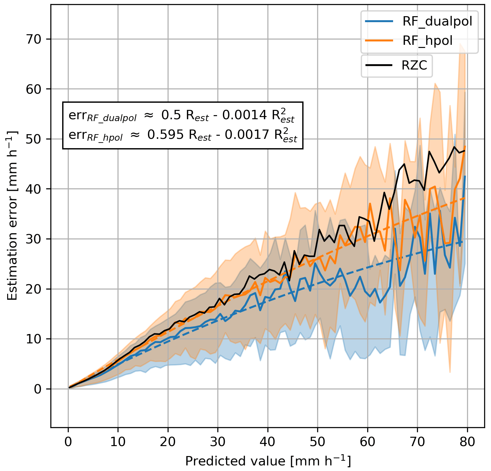
Figure 12Absolute error of the precipitation estimate as a function of the precipitation estimate, evaluated over five iterations of a five-fold cross-validation, for the two RF models. The colored semi-transparent area corresponds to the Q25–Q75 interquantile, the solid lines to the mean and the dashed line to a polynomial fit, whose formulation is shown in the box on the left. The solid black line corresponds to the average error of the RZC model which is shown as a reference. All quantiles and means have been obtained using a discretization on the predicted values with a step of 1 mm h−1.
The RF QPE method derived from the database has been adapted to a quasi-operational framework in order to generate 5 min QPE maps at the same temporal and spatial resolution as the RZC product. The main steps remain identical, namely, the spatial averaging of input features to 1 km2, followed by a vertical aggregation to the ground using a logarithmic profile (with ), and finally the use of the trained RF to predict precipitation intensities at the ground. This final estimate is then converted into 256 digital numbers (byte format) using the same lookup table used for the encoding of the RZC product. However, a few modifications were necessary in order to improve the spatial structure of the final RF product and take into account the change in temporal support between the database and the 5 min QPE maps.
5.1 Local outlier removal and low-pass filtering
The estimated QPE is generally noisier in space than the standard RZC product. This can be explained by the inherent discretization performed by the RF regression method and by the addition of new weakly intercorrelated input features. To alleviate this issue, two operations are performed successively. First a 3×3 pixel local outlier removal is applied: in every 3×3 neighborhood, if the z value (precipitation intensity standardized within its neighborhood) of a pixel is larger than 3 or lower than −3, its value is replaced by the mean in the neighborhood. The second step is a low-pass filtering, for which two approaches have been considered:
-
A simple 2D Gaussian filtering with a standard deviation of σ=0.5 km (0.5 pixel) is the first approach. An explanation regarding this choice of σ is given in Appendix D.
-
An advection-correction method in which two consecutive 5 min QPE fields are decomposed into a sequence of five fields at a resolution of 1 min which are then averaged (Appendix 2 of Anagnostou and Krajewski, 1999) is the second approach. The Lukas–Kanade optical flow method as implemented in pysteps (Pulkkinen et al., 2019) was used to derive the motion vectors of the precipitation fields. In the following the term RF_dualpol_AC will be used for the RF product obtained with dual-polarization inputs and smoothed with the advection-correction method.
A comparison of these two methods is shown in Fig. 13. The advection-corrected field looks much smoother, and the intense precipitation cells are larger, although in fact their cores tend to have weaker intensities.
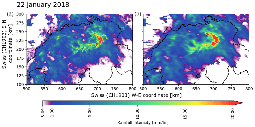
Figure 13Resulting QPE field on a case of widespread snowfall, on the left with Gaussian smoothing (σ=0.5 pixels) and on the right with advection correction.
5.2 Temporal disaggregation
The RF method has been trained from the database to predict precipitation intensities over a 10 min period since it is the smallest available timescale of gauge observations. A disaggregation of the 10 min estimate delivered by the RF method is thus necessary in order to match the 5 min resolution of RZC. In our case we base the disaggregation on the Z–R relationship used by MeteoSwiss in its RZC product (Joss et al., 1998):
where zh is the linear reflectivity (in mm6 m−3) and RZR the estimated rain intensity (in mm h−1).
At a every time step t, the disaggregation is done in the following way:
-
The input features to the RF are computed by taking the average of the two latest 5 min time steps.
-
The 10 min estimate is computed with the RF model trained on the database.
-
The 5 min RF estimate is obtained by using the fraction of , estimated from zt (with Eq. 9), to , estimated from .
Figure 14 shows examples of generated QPE fields for two very different precipitation events. The spatial structure of the RF fields looks realistic with no visible radar artifacts such as bright band (especially for the 22 January event, when mixed-phase precipitation is omnipresent) or influence from ground clutter. Despite the Gaussian smoothing the RF fields look somewhat more discontinuous than RZC and particularly CPC (which is naturally smooth due to the kriging procedure). For these two examples, the RF field looks like an intermediate stage between RZC and CPC, with weaker and more localized precipitation cores than RZC. This is however not a systematic behavior.
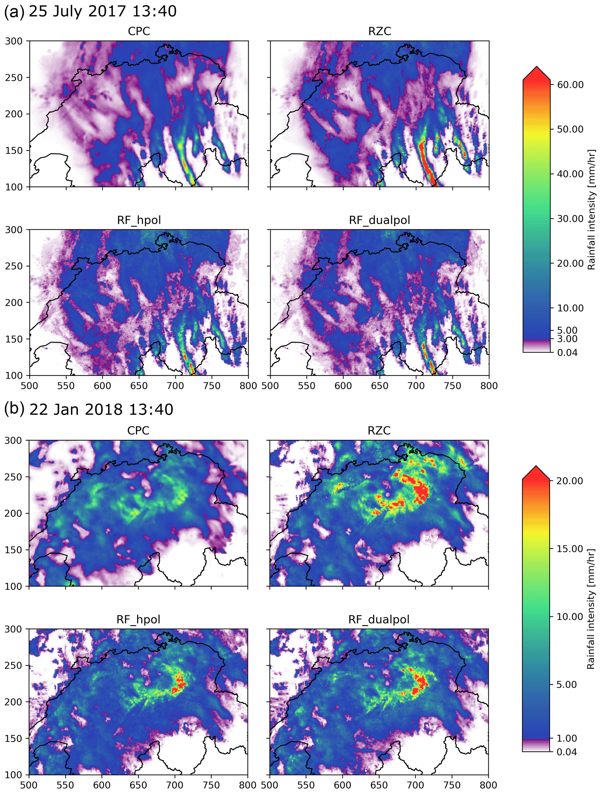
Figure 14Two examples of precipitation fields generated with RZC, CPC, RF_dualpol and RF_hpol (both with Gaussian smoothing): (a) strong convection on 25 July 2017 during a typical summertime barometric swamp. The color scale is divided in a linear progression in purple tones for low precipitation and a logarithmic progression from blue to green above a certain threshold. (b) Heavy snowfall event during a warm front crossing of Switzerland on 22 January 2018.
5.3 Case studies
Six precipitation events typical of Switzerland are considered, of which two correspond to widespread winter snow events (warm front on 22 January 2018 and cold front on 29 January 2020), two to summer convection with heavy precipitation (thermal convection on 25 July 2017 and cold front convection on 6 August 2019), and two to cold front situations in autumn with mainly stratiform precipitation (27 October 2018 and 15 October 2019). All events last for 24 h from midnight to midnight. To ensure an unbiased estimate of the performance, the RF models used for prediction have been trained after filtering out all input data from these 6 d.
The performance of all QPE methods is given in Fig. 15 in the form of a color-coded table. The best-performing QPE is almost systematically CPC.CV. Since this method uses also ground measurements, the comparison with pure radar products such as RZC and the RF QPE is not fair, but the performance of CPC.CV can be considered as an asymptotic ideal performance to which the best-possible radar QPE should tend. It appears that RF_dualpol (with Gaussian smoothing) has a lower RMSE than RZC for four out of six events (and equal RMSE for the two others), a lower scatter than RZC for five out of six events, a better logBias than RZC for five out of six events and a lower ED for four out of six events. In contrast, the performance of RF_dualpol_AC, the RF dual-polarization QPE with a posteriori advection correction (Sect. 5.1), is much poorer, and it often overestimates precipitation as can be seen by the larger logBias. In fact this overestimation is limited to small precipitation intensities, which indicates that the smoothing effect is too strong as the high values in the precipitation cores tend to leak towards the margins of the precipitation system. The performance of the single polarization RF_hpol model is almost systematically worse than RF_dualpol and as such can not really be used as an alternative to RZC. Most likely in the absence of polarimetric information, the RF algorithm is not able to overcome the absence of an additional VPR and local bias corrections as are applied to the RZC product. When looking at the performance for different precipitation ranges, the RF models tend to produce larger precipitation intensities for low observed precipitation with respect to RZC. In most of the cases, this is rather a good sign since RZC tends to underestimate at these ranges, but in some cases (15 October and 6 August 2019) it leads to the overestimation of weak precipitation. This can be explained by the natural tendency of the RF to overestimate weak responses, which is not totally compensated for by the a posteriori bias correction. For observed intense precipitation above 10 mm h−1, RZC is clearly underestimating for all events. RF_dualpol still underestimates but to a significantly lesser amount, and the relative decrease in logBias with respect to RZC ranges from 10 % to 40 % depending on the event. The only event in which the performance of RF_dualpol is problematic is 6 August 2019, when it has a clear tendency to overestimate weak and intermediate (up to 10 mm h−1) precipitation. Nevertheless, it is necessary to keep in mind the large difference in the spatial support of the rain gauge and the radar, which makes a direct comparison difficult. As the radar provides an average over a much larger area than the rain gauge, it would not be surprising that the estimated values are underestimated with respect to the gauge in case of intense precipitation.
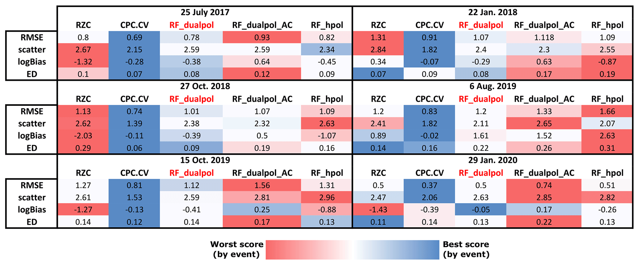
Figure 15Evaluation scores at hourly resolution for the RZC, CPC.CV, RF_dualpol (with Gaussian smoothing), RF_dualpol_AC (advection-corrected) and RF_hpol (with Gaussian smoothing) methods for the six events using the rain gauge measurements from all Swiss stations as reference. Green colors correspond to good relative performance and red colors to poor relative performance.
In this work we propose a new data-based QPE method for Switzerland that is able to generate 2D estimates of precipitation intensities over a 1 km2 grid, every 5 min, in real time.
The first step of this work involved the creation of a large database comprising 4 years of radar measurements from the five operational polarimetric weather radars, simulations from the operational COSMO NWP (numerical weather prediction) model and gauge measurements from the 288 operational rain gauges, aggregated to a common spatial and temporal representation.
This database was then used to adjust and train a random forest (RF) algorithm able to predict the gauge observation at the ground from the radar observations aloft. Compared to other machine learning regression models, RF has the advantage of being easy to parallelize, being very fast for prediction in real-time application and never generating non-physical precipitation amounts. Since machine learning methods such as RF typically require the response and the input features to have the same dimensions, the observations aloft are aggregated to the ground using a weighted average that depends exponentially on the altitude of each observation. The relative importance of each input feature was assessed using a random shuffling scheme, and the final choice of features includes nine features, which are by order of importance the horizontal reflectivity Zh, the vertical reflectivity Zv, the specific differential phase shift Kdp, the fraction of observations that come from each of the five radars, the co-polar correlation coefficient ρhv, the spectral width Sw, the temperature from the COSMO model, the static radar visibility and the radar gate altitude. It was observed that the trained RF method has a natural tendency to overestimate weak precipitation and underestimate strong precipitation, which is a well-known behavior of many machine learning methods. This tendency can be alleviated to a large extent with an a posteriori bias-correction method that relies on a fit between observed precipitation and predicted precipitation. The final model includes the following hyperparameters: (1) the slope in the exponential altitude weighting of the input features, (2) the number of trees, (3) the maximum depth of the trees, (4) the number of variables randomly chosen at each split and (5) the type of a posteriori bias correction. By running a five-fold cross-validation for every parameter combination, it was observed that the performance differs greatly as a function of the precipitation intensity range and the type of metrics that is used. There is thus no single best choice but a good trade-off could be found with a multi-criterion decision scheme. The learning curve computed for this fine-tuned algorithm reveals that the training data are sufficient but that the required data are quite large in regard of the small number of input features. This result can be explained by the intrinsic loss of information due to the aggregation of the gauge data to the spatial and temporal support of the gauge and the inherent noisiness of some of the radar variables.
A comparison of this new algorithm with RZC, the current single-polarization QPE product of MeteoSwiss, reveals that it decreases significantly the estimation error and bias in most areas of Switzerland. This is particularly true in the central Alpine regions, where RZC tends to underestimate. Nevertheless, even though the bias-correction method solves to a large extent the issue of underestimating heavy precipitation, for which the RF QPE is generally better than RZC, the RF algorithm still has a visible tendency to overestimate weak precipitation. When training an RF QPE without the polarimetric information, the performance is generally much poorer and worse than or comparable to RZC. Some effort was also invested in the computation of an error model which allows us to estimate the error associated the predicted precipitation intensities. This model reveals that the polarimetric information reduces the error clearly when compared with RZC or RF without polarimetry.
To be able to provide 5 min precipitation maps, the algorithm was adapted with a disaggregation scheme that predicts 5 min estimates from 10 min averaged input features (which is the temporal support of gauge observations and hence the one used for training the RF algorithm). This scheme relies on the Z–R relationship used in the operational RZC model. It was observed that the resulting QPE fields could display locally sharp discontinuities which are not visible in RZC, which is generally smoother. These discontinuities can be explained by the use of new additional input variables in the QPE, as well as the discretization performed by the RF regression. To improve the spatial structure of the output, the QPE scheme was complemented with a 3×3 local outlier removal filter and a Gaussian low-pass filter with σ = 0.5 km. A series of six case studies for typical precipitation events over Switzerland reveals that the generated precipitation looks realistic and gives a better performance than RZC for five out of six events.
This new RF QPE method has proven to deliver promising results and has the advantage of replacing many of the a posteriori corrections required by RZC (global and local bias corrections, VPR correction) by one single fast estimation step. Further work is required to improve its capability to predict weak precipitation intensities, which might require a more sophisticated aggregation scheme of radar observations aloft. This QPE algorithm offers vast perspectives for operational real-time applications, indeed it is fast (less than a minute of computation every 5 min), and because of its simple structure (ensemble of decision trees), the RF regressor can easily be used in the operational MeteoSwiss framework, provided the radar variables are transformed into input features accordingly. In parallel, the database will periodically be updated with newly acquired data, and the RF regressor will be retrained. Ultimately this new RF QPE should serve as input for the CPC algorithm which provides the best possible QPE estimate over Switzerland by merging radar QPE and gauge data (Sideris et al., 2014).
To create a database of 4 years of radar data, more than 10 million radar PPI scans have to be processed (five radars, 20 elevations every 5 min). Because of this, it is computationally impossible to use an advanced Kdp estimation method, such as a Kalman filter method (Schneebeli et al., 2014) or a Gaussian-mixture regression (Wen et al., 2019). Hence a simple method is used in this study which is also used in Wolfensberger et al. (2018) and is similar to the one in Timothy et al. (1999). The raw total differential phase shift Ψdp is first corrected for the system offset and then filtered with a moving median filter to give an estimate of the total differential phase shift on propagation Φdp. To estimate Kdp, which is half of the slope of Φdp, a moving linear regression is used, in which the slope is estimated in a moving window. For the sake of consistency the same window length is used both for the median filtering of the phase and the linear regression. Tests showed that the best results are obtained by using a large window of 6 km.
Concerning Ah, we use the ZPHI method (Testud et al., 2000), in liquid phase only. The COSMO temperature is used to identify the height of the freezing level. Attenuation is neglected in the solid phase (i.e., Ah is always zero above the freezing level). In the liquid phase, we use constant values of γ=0.08 and b=0.64884, as provided by default in the Pyart package (Helmus and Collis, 2016).
Figures B1 and B2 show the RMSEs for all precipitation intensities and only high precipitation intensities, respectively. It clearly shows that even at large precipitation intensities, using no bias correction (first column) gives quite large errors. These plots also show that even when considering only RMSE, it is difficult to find a good trade-off in the choice of hyperparameters.
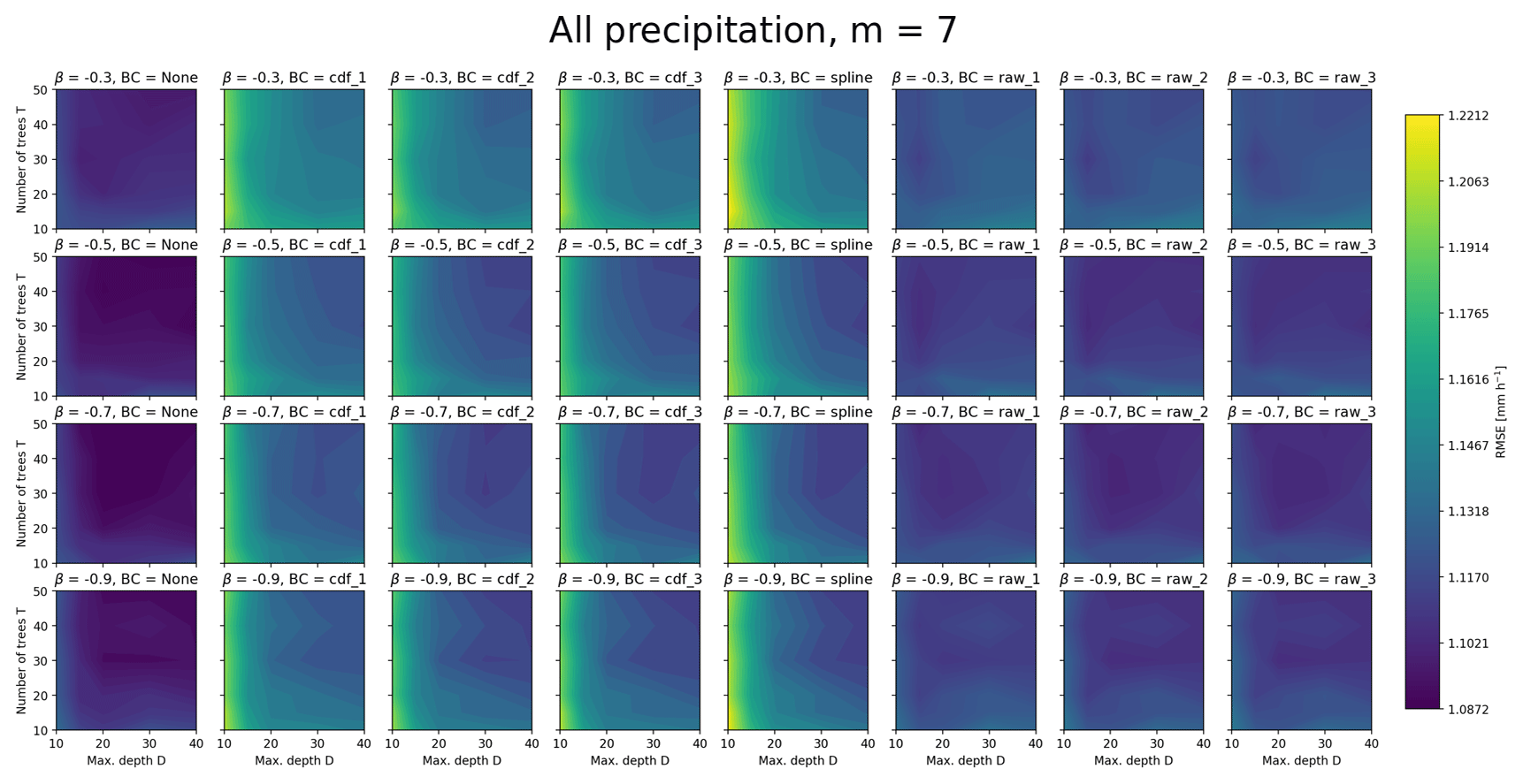
Figure B1Overall RMSEs for all observations as a function of number of trees, maximum depth, β parameter and bias-correction method. The maximum number of randomly chosen variables at each split is here set to seven.
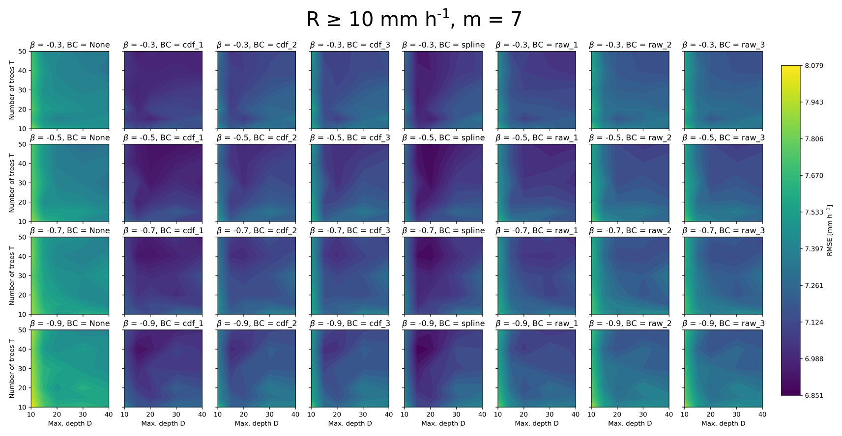
Figure B2Overall RMSEs for observations ≥10 mm h−1 as a function of number of trees, maximum depth, β parameter and bias-correction method. The maximum number of randomly chosen variables at each split is here set to seven.
Figure C1 shows the overall cross-validation performance of RZC, CPC.CV, RF_dualpol and RF_hpol over the whole database, separated by precipitation phase and intensity.

Figure C1Five-fold cross-validation performance of RZC, CPC.CV, RF_dualpol and RF_hpol for different observed precipitation ranges for liquid and solid or mixed precipitation and for both together (which includes all additional observations from stations where no temperature measurement is available). The y scale is different for all precipitation ranges since the scores are significantly different.
The optimal σ value in the Gaussian smoothing of the 2D QPE fields has been chosen by analyzing the overall performance in terms of RMSE and linear bias during the six representative precipitation events as a function of the value of σ. Intuitively, if the smoothing is too intense, the natural tendency of the RF to overestimate weak precipitation and underestimate strong precipitation could be worsened. The results, displayed in Fig. D1, show that increasing σ leads to a decrease in the RMSE but also to a sharp increase (in magnitude) in the bias. A value of σ=0.5 km seems to be a good trade-off since it leads to a comparatively low increase in bias for a comparatively large decrease in RMSE.

Figure D1Hourly RMSE and linear bias (average of estimated versus observed value) as a function of the value of σ (a) for low intensities and (b) for higher intensities.
Data and code are available on request by contacting the authors.
DW designed and implemented the QPE algorithm, performed all experiments detailed in this work and wrote the manuscript. AB, MG, MB and UG contributed to the design and discussion of the work, as well as to the writing of the manuscript.
The authors declare that they have no conflict of interest.
The authors would like to thank Ioannis Sideris for all help regarding the CPC algorithm and its products. The authors are also grateful to Marco Boscacci and Jordi Figueras i Ventura for the advice regarding all MeteoSwiss operational products.
This paper was edited by Gianfranco Vulpiani and reviewed by Irene Crisologo and one anonymous referee.
Anagnostou, E. N. and Krajewski, W. F.: Real-Time Radar Rainfall Estimation. Part I: Algorithm Formulation, J. Atmos. Ocean. Tech., 16, 189–197, https://doi.org/10.1175/1520-0426(1999)016<0189:RTRREP>2.0.CO;2, 1999. a
Anagnostou, M. N., Kalogiros, J., Anagnostou, E. N., Tarolli, M., Papadopoulos, A., and Borga, M.: Performance evaluation of high-resolution rainfall estimation by X-band dual-polarization radar for flash flood applications in mountainous basins, J. Hydrol., 394, 4–16, https://doi.org/10.1016/j.jhydrol.2010.06.026, 2010. a
Baldauf, M., Seifert, A., Förstner, J., Majewski, D., Raschendorfer, M., and Reinhardt, T.: Operational convective-scale numerical weather prediction with the COSMO model: description and sensitivities, Mon. Weather Rev., 139, 3887–3905, https://doi.org/10.1175/MWR-D-10-05013.1, 2011. a
Barton, Y., Sideris, I. V., Germann, U., and Martius, O.: A method for real-time temporal disaggregation of blended radar–rain gauge precipitation fields, Meteorol. Appl., 27, e1843, https://doi.org/10.1002/met.1843, 2020. a, b
Besic, N., Figueras i Ventura, J., Grazioli, J., Gabella, M., Germann, U., and Berne, A.: Hydrometeor classification through statistical clustering of polarimetric radar measurements: a semi-supervised approach, Atmos. Meas. Tech., 9, 4425–4445, https://doi.org/10.5194/amt-9-4425-2016, 2016. a
Breiman, L.: Random Forests, Mach. Learn., 45, 5–32, https://doi.org/10.1023/A:1010933404324, 2001. a, b
Breiman, L., Friedman, J. H., Olshen, R. A., and Stone, C. J.: Classification and Regression Trees, Statistics/Probability Series, Wadsworth Publishing Company, Belmont, California, USA, 1984. a
Buisán, S. T., Earle, M. E., Collado, J. L., Kochendorfer, J., Alastrué, J., Wolff, M., Smith, C. D., and López-Moreno, J. I.: Assessment of snowfall accumulation underestimation by tipping bucket gauges in the Spanish operational network, Atmos. Meas. Tech., 10, 1079–1091, https://doi.org/10.5194/amt-10-1079-2017, 2017. a
Bukovčić, P., Ryzhkov, A., Zrnić, D., and Zhang, G.: Polarimetric Radar Relations for Quantification of Snow Based on Disdrometer Data, J. Appl. Meteorol. Clim., 57, 103–120, https://doi.org/10.1175/JAMC-D-17-0090.1, 2018. a
Chapon, B., Delrieu, G., Gosset, M., and Boudevillain, B.: Variability of rain drop size distribution and its effect on the Z-R relationship: a case study for intense Mediterranean rainfall, Atmos. Res., 87, 52–65, 2008. a
Cleveland, R. B., Cleveland, W. S., McRae, J. E., and Terpenning, I.: STL: A Seasonal-Trend Decomposition Procedure Based on Loess, J. Off. Stat., 6, 3–73, 1990. a
Cybenko, G.: Approximation by superpositions of a sigmoidal function, Math. Control Signal., 2, 303–314, 1989. a
Doms, G., Förstner, J., Heise, E., Herzog, H., Mironov, D., Raschendorfer, M., Reinhardt, T., Ritter, B., Schrodin, R., Schulz, J.-P., and Vogel, G.: A description of the nonhydrostatic regional COSMO model, Part II: Physical Parameterization, available at: http://www.cosmo-model.org/content/model/documentation/core/cosmo_physics_4.20.pdf (last access: 4 August 2015), 2011. a
Edgeworth, M.: XXII. On a new method of reducing observations relating to several quantities, The London, Edinburgh, and Dublin Philosophical Magazine and Journal of Science, 25, 184–191, https://doi.org/10.1080/14786448808628170, 1888. a
Fujiyoshi, Y., Endoh, T., yamada, T., Tsuboki, K., Tachibana, Y., and Wakahama, G.: Determination of a Z-R relationship for snowfall using a radar and high sensitivity snow gauges, J. Appl. Meteorol., 29, 147–152, 1990. a
Gabella, M. and Perona, G.: Simulation of the Orographic Influence on Weather Radar Using a Geometric Optics Approach, J. Atmos. Ocean. Tech., 15, 1485–1494, https://doi.org/10.1175/1520-0426(1998)015<1485:SOTOIO>2.0.CO;2, 1998. a
Gabella, M., Speirs, P., Hamann, U., Germann, U., and Berne, A.: Measurement of Precipitation in the Alps Using Dual-Polarization C-Band Ground-Based Radars, the GPM Spaceborne Ku-Band Radar, and Rain Gauges, Remote Sensing, 9, 1147, https://doi.org/10.3390/rs9111147, 2017. a, b
Germann, U. and Joss, J.: Mesobeta profiles to extrapolate radar precipitation measurements above the Alps to the ground level, J. Appl. Meteorol., 41, 542–557, 2002. a
Germann, U., Galli, G., Boscacci, M., and Bolliger, M.: Radar precipitation measurement in a mountainous region, Q. J. Roy. Meteor. Soc., 132, 1669–1692, https://doi.org/10.1256/qj.05.190, 2006. a, b, c, d, e
Germann, U., Berenguer, M., Sempere-Torres, D., and Zappa, M.: REAL – Ensemble radar precipitation estimation for hydrology in a mountainous region, Q. J. Roy. Meteor. Soc., 135, 445–456, https://doi.org/10.1002/qj.375, 2009. a
Germann, U., Boscacci, M., Gabella, M., and Sartori, M.: Peak Performance: Radar design for prediction in the Swiss Alps, Meteorological Technology International, Dorking, Surrey, UK, 42–45, 2015. a
Han, H., Guo, X., and Yu, H.: Variable selection using Mean Decrease Accuracy and Mean Decrease Gini based on Random Forest, in: 2016 7th IEEE International Conference on Software Engineering and Service Science (ICSESS), Beijing, China, 26–28 August 2016, 219–224, https://doi.org/10.1109/ICSESS.2016.7883053, 2016. a
Helmus, J. and Collis, S.: Disaggregation of daily rainfall, Journal of Open Research Software, e25, 1–6, https://doi.org/10.5334/jors.119, 2016. a
Hooper, D. A., McDonald, A. J., Pavelin, E., Carey-Smith, T. K., and Pascoe, C. L.: The signature of mid-latitude convection observed by VHF wind-profiling radar, Geophys. Res. Lett., 32, L04808, https://doi.org/10.1029/2004GL020401, 2005. a
Houze Jr., R. A.: Orographic effects on precipitating clouds, Rev. Geophys., 50, RG1001, https://doi.org/10.1029/2011RG000365, 2012. a
Joss, J., Schädler, B., Galli, G., Cavalli, R., Boscacci, M., Held, E., Della Bruna, G., Kappenberger, G., Nespor, V., and Spiess, R.: Operational use of radar for precipitation measurements in Switzerland, vdf Hochschulverlag AG, ETH Zürich, Switzerland, available at: https://www.meteosuisse.admin.ch/content/dam/meteoswiss/fr/Mess-und-Prognosesysteme/doc/meteoswiss_operational_use_of_radar.pdf (last access: 14 September 2020), 1998. a, b, c
Kitchen, M. and Blackall, R. M.: Representativeness errors in comparisons between radar and gauge measurements of rainfall, J. Hydrol., 134, 13–33, 1992. a
Kochendorfer, J., Rasmussen, R., Wolff, M., Baker, B., Hall, M. E., Meyers, T., Landolt, S., Jachcik, A., Isaksen, K., Brækkan, R., and Leeper, R.: The quantification and correction of wind-induced precipitation measurement errors, Hydrol. Earth Syst. Sci., 21, 1973–1989, https://doi.org/10.5194/hess-21-1973-2017, 2017. a
Belgiu, M. and Drăguţ, L.: Random forest in remote sensing: A review of applications and future directions, ISPRS Journal of Photogrammetry and Remote Sensing, 114, 24–31, https://doi.org/10.1016/j.isprsjprs.2016.01.011, 2016. a
Mapiam, P., Sharma, A., and Sriwongsitanon, N.: Defining the Z–R Relationship Using Gauge Rainfall with Coarse Temporal Resolution: Implications for Flood Forecasting, J. Hydraul. Eng., 19, p. 04014003 https://doi.org/10.1061/(ASCE)HE.1943-5584.0000616, 2014. a
Marshall, J. S. and Palmer, W. M.: The distribution of raindrops with size, J. Meteor., 5, 165–166, 1948. a
Meek, C., Thiesson, B., and Heckerman, D.: The Learning-Curve Sampling Method Applied to Model-Based Clustering, J. Mach. Learn. Res., 2, 397–418, https://doi.org/10.1162/153244302760200678, 2002. a
Morin, E. and Gabella, M.: Radar-based quantitative precipitation estimation over Mediterranean and dry climate regimes, J. Geophys. Res., 112, D20108, https://doi.org/10.1029/2006JD008206, 2007. a
Orellana-Alvear, J., Célleri, R., Rollenbeck, R., and Bendix, J.: Optimization of X-Band Radar Rainfall Retrieval in the Southern Andes of Ecuador Using a Random Forest Model, Remote Sensing, 11, 1632, https://doi.org/10.3390/rs11141632, 2019. a
Panziera, L., Gabella, M., Germann, U., and Martius, O.: A 12‐year radar‐based climatology of daily and sub‐daily extreme precipitation over the Swiss Alps, Int. J. Climatol., 38, 3749–3769, https://doi.org/10.1002/joc.5528, 2017. a
Pedregosa, F., Varoquaux, G., Gramfort, A., Michel, V., Thirion, B., Grisel, O., Blondel, M., Prettenhofer, P., Weiss, R., Dubourg, V., Vanderplas, J., Passos, A., Cournapeau, D., Brucher, M., Perrot, M., and Duchesnay, E.: Scikit-learn: Machine Learning in Python, J. Mach. Learn. Res., 12, 2825–2830, 2011. a
Praz, C., Roulet, Y.-A., and Berne, A.: Solid hydrometeor classification and riming degree estimation from pictures collected with a Multi-Angle Snowflake Camera, Atmos. Meas. Tech., 10, 1335–1357, https://doi.org/10.5194/amt-10-1335-2017, 2017. a
Pulkkinen, S., Nerini, D., Pérez Hortal, A. A., Velasco-Forero, C., Seed, A., Germann, U., and Foresti, L.: Pysteps: an open-source Python library for probabilistic precipitation nowcasting (v1.0), Geosci. Model Dev., 12, 4185–4219, https://doi.org/10.5194/gmd-12-4185-2019, 2019. a
Rao, T. N., Radhakrishna, B., Mohan Satyanarayana, T., and Satheesh Kumar, S.: The exchange across the tropical tropopause in overshooting convective cores, Ann. Geophys., 28, 113–122, https://doi.org/10.5194/angeo-28-113-2010, 2010. a
Rizzo, M. L. and Székely, G. J.: Energy distance, WIREs Computational Statistics, 8, 27–38, https://doi.org/10.1002/wics.1375, 2016. a
Ryzhkov, A., Diederich, M., Zhang, P., and Simmer, C.: Potential Utilization of Specific Attenuation for Rainfall Estimation, Mitigation of Partial Beam Blockage, and Radar Networking, J. Atmos. Ocean. Tech., 31, 599–619, https://doi.org/10.1175/JTECH-D-13-00038.1, 2014. a, b
Ryzhkov, A. V. and Zrnic, D. S.: Discrimination between rain and snow with a polarimetric radar, J. Appl. Meteorol., 37, 1228–1240, 1998. a
Ryzhkov, A. V., Schuur, T. J., Burgess, D. W., Heinselman, P. L., Giangrande, S. E., and Zrnic, D. S.: The joint polarization experiment, polarimetric rainfall measurements and hydrometeor classification, B. Am. Meteorol. Soc., 86, 809–824, https://doi.org/10.1175/BAMS-86-6-809, 2005. a
Schneebeli, M., Grazioli, J., and Berne, A.: Improved estimation of the specific differential phase shift using a compilation of Kalman filter ensembles, IEEE T. Geosci. Remote Sens., 52, 5137–5149, https://doi.org/10.1109/TGRS.2013.2287017, 2014. a
Seifert, A., Blahak, U., Stephan, K., Baldauf, M., and Schulz, J.-P.: Documentation of the Changes in the COSMO-Model, Version 4.21, available at: http://www.cosmo-model.org/content/model/releases/histories/cosmo_4.21.htm (last access: 4 August 2015), 2011. a
Sideris, I. V., Gabella, M., Erdin, R., and Germann, U.: Real-time radar–rain-gauge merging using spatio-temporal co-kriging with external drift in the alpine terrain of Switzerland, Q. J. Roy. Meteor. Soc., 140, 1097–1111, https://doi.org/10.1002/qj.2188, 2014. a, b, c, d
Speirs, P., Gabella, M., and Berne, A.: A comparison between the GPM dual-frequency precipitation radar and ground-based radar precipitation rate estimates in the Swiss Alps and Plateau, J. Hydrometeorol., 18, 1247–1269, https://doi.org/10.1175/JHM-D-16-0085.1, 2017. a
Suter, S., Konzelmann, T., Mühlhäuser, C., Begert, M., and Heimo, A.: SwissMetNet – the new automatic meteorological network of Switzerland: transition from old to new network, data management and first results, in: Proceedings of the 4th International Conference on Experiences with Automatic Weather Stations (4th ICEAWS), Lisbon, Portugal, 24–26 May 2006, vol. 24, 2006. a
Testud, J., Le Bouar, E., Obligis, E., and Ali-Mehenni, M.: The rain profiling algorithm applied to polarimetric weather radar, J. Atmos. Ocean. Tech., 17, 332–356, 2000. a
Timothy, K. I., Iguchi, T., Ohsaki, Y., Horie, H., Hanado, H., and Kumagai, H.: Test of the Specific Differential Propagation Phase Shift (KDP) Technique for Rain-Rate Estimation with a Ku-Band Rain Radar, J. Atmos. Ocean. Tech., 16, 1077–1091, https://doi.org/10.1175/1520-0426(1999)016<1077:TOTSDP>2.0.CO;2, 1999. a
Tokay, A., Hartmann, P., Battaglia, A., Gage, K. S., Clark, W. L., and Williams, C. R.: A field study of reflectivity and Z-R relations using vertically pointing radars and disdrometers, J. Atmos. Ocean. Tech., 26, 1120–1134, https://doi.org/10.1175/2008JTECHA1163.1, 2009. a
van den Heuvel, F., Foresti, L., Gabella, M., Germann, U., and Berne, A.: Learning about the vertical structure of radar reflectivity using hydrometeor classes and neural networks in the Swiss Alps, Atmos. Meas. Tech., 13, 2481–2500, https://doi.org/10.5194/amt-13-2481-2020, 2020. a
Verrier, S., Barthès, L., and Mallet, C.: Theoretical and empirical scale dependency of Z-R relationships: Evidence, impacts, and correction, J. Geophys. Res., 118, 7435–7449, https://doi.org/10.1002/jgrd.50557, 2013. a
Wen, G., Fox, N. I., and Market, P. S.: A Gaussian mixture method for specific differential phase retrieval at X-band frequency, Atmos. Meas. Tech., 12, 5613–5637, https://doi.org/10.5194/amt-12-5613-2019, 2019. a
Wen, G., Fox, N. I., and Market, P. S.: A Gaussian mixture method for specific differential phase retrieval at X-band frequency, Atmos. Meas. Tech., 12, 5613–5637, https://doi.org/10.5194/amt-12-5613-2019, 2018. a
Wolfensberger, D., Gabella, M., Boscacci, U., Berne, A., and Germann, U.: Potential use of specific differential propagation phase delay for the retrieval of rain rates in strong convection over Switzerland, in: Proc. 3rd International Workshop on Precipitation In Urban Areas (UrbanRain), Pontresina, Switzerland, 5–7 December 2018. a
Zhang, G. and Lu, Y.: Bias-corrected random forests in regression, J. Appl. Stat., 39, 151–160, https://doi.org/10.1080/02664763.2011.578621, 2012. a
Zrnic, D. S. and Ryzhkov, A. V.: Polarimetry for weather surveillance radars, B. Am. Meteorol. Soc., 80, 389–406, 1999. a
The temporal resolution of the COSMO model is much higher, but since the data amount is huge, 3D archives are kept only at hourly resolution.
This corresponds to one tip of a tipping bucket rain gauge and is the maximum resolution of all rain gauges.
−0.2, 0.4, 1.0, 1.6, 2.5, 3.5, 4.5, 5.5, 6.5, 7.5, 8.5, 9.5, 11.0, 13.0, 16.0, 20.0, 25.0, 30.0, 35.0 and 40.0∘.
As stated previously, the radar fraction is decomposed into five features, one for every radar.
- Abstract
- Introduction
- Collocated gauge–radar database
- QPE computation
- Fitting of a QPE model and results
- Generation of 5 min QPE maps
- Conclusions
- Appendix A: Computation of Kdp and Ah
- Appendix B: Cross-validation results
- Appendix C: Overall performance at different precipitation ranges
- Appendix D: Choice of σ in the Gaussian smoothing
- Code and data availability
- Author contributions
- Competing interests
- Acknowledgements
- Review statement
- References