the Creative Commons Attribution 4.0 License.
the Creative Commons Attribution 4.0 License.
 | 04 May 2021
The INFRA-EAR: a low-cost mobile multidisciplinary measurement platform for monitoring geophysical parameters
Olivier F. C. den Ouden
Jelle D. Assink
Cornelis D. Oudshoorn
Dominique Filippi
Läslo G. Evers
Geophysical studies and real-time monitoring of natural hazards, such as volcanic eruptions or severe weather events, benefit from the joint analysis of multiple geophysical parameters. However, typical geophysical measurement platforms still provide logging solutions for a single parameter, due to different community standards and the higher cost per added sensor.
In this work, the Infrasound and Environmental Atmospheric data Recorder (INFRA-EAR) is presented, which has been designed as a low-cost mobile multidisciplinary measurement platform for geophysical monitoring. In particular, the platform monitors infrasound but concurrently measures barometric pressure, accelerations, and wind flow and uses the Global Positioning System (GPS) to position the platform. Due to its digital design, the sensor platform can be readily integrated with existing geophysical data infrastructures and be embedded in geophysical data analysis. The small dimensions and low cost per unit allow for unconventional, experimental designs, for example, high-density spatial sampling or deployment on moving measurement platforms. Moreover, such deployments can complement existing high-fidelity geophysical sensor networks. The platform is designed using digital micro-electromechanical system (MEMS) sensors embedded on a printed circuit board (PCB). The MEMS sensors on the PCB are a GPS, a three-component accelerometer, a barometric pressure sensor, an anemometer, and a differential pressure sensor. A programmable microcontroller unit controls the sampling frequency of the sensors and data storage. A waterproof casing is used to protect the mobile platform against the weather. The casing is created with a stereolithography (SLA) Formlabs 3D printer using durable resin.
Thanks to low power consumption (9 Wh over 25 d), the system can be powered by a battery or solar panel. Besides the description of the platform design, we discuss the calibration and performance of the individual sensors.
- Article
(4213 KB) - Full-text XML
- BibTeX
- EndNote


Real-time monitoring of natural hazards, such as volcanic eruptions or severe weather events benefit from the joint analysis of multiple geophysical parameters. However, geophysical measurement platforms are typically designed to measure a single parameter, due to different community standards and the higher cost per added sensor. The quality and robustness of geophysical measuring equipment generally scale with price, due to higher material costs and research and development (R&D) expenses. In addition, the deployment of such equipment comes with complex deployment and calibration procedures and requires the presence of a robust power and data infrastructure.
Geophysical institutes often place multiple sensor platforms co-located. Meteorological institutes, for example, measure various meteorological parameters for comparison, which improves the weather observations and weather forecast models. The Comprehensive Nuclear-Test-Ban Treaty Organization (CTBTO) performs various geophysical measurements at its measurement sites where possible. The International Monitoring System (IMS), which is in place for verification of the Comprehensive Nuclear Test Ban Treaty (CTBT), performs continuous seismic, hydroacoustic, infrasonic, and radionuclide measurements (Marty, 2019). In addition, the IMS infrasound arrays and radionuclide facilities host auxiliary meteorological equipment, as this data facilitates the review of the primary IMS data streams. Besides its use for verifying the CTBT, it has also been shown that a multi-instrumental observation network such as the IMS can provide useful information on the vertical dynamic structure of the middle and upper atmosphere, in particular when paired with complementary upper atmospheric remote sensing techniques such as lidar (Blanc et al., 2018). Other studies that involve the analysis of multiple geophysical parameters include seismo-acoustic analyses of explosions (Assink et al., 2018; Averbuch et al., 2020), earthquakes (Shani-Kadmiel et al., 2018), and volcanoes (Green et al., 2012).
National weather services, such as the Royal Netherlands Meteorological Institute (KNMI), have expressed an interest in measuring weather on a local scale to inform and warn citizens of extreme weather. In addition, such measurements allow for higher-resolution measurements of sub-grid scale atmospheric dynamics, which will contribute to the improvement of short-term and nowcasting weather forecasts (Manobianco and Short, 2001; Lammel, 2015). Therefore it became part of a low-cost citizen weather station program to increase the spatial resolution of conventional numerical weather prediction models. In the Netherlands, over 300 of those weather stations contribute to a global citizen science project, Weather Observations Website (WOW) (Garcia-Marti et al., 2019; Cornes et al., 2020). Nonetheless, due to the required infrastructure of the equipment, many platforms are spatially static. Having a low-cost multidisciplinary mobile sensor platform allows for high-resolution spatial sampling and complements existing high-fidelity geophysical sensor networks (e.g., buoys in the open ocean, Grimmett et al., 2019; and stratospheric balloons, Poler et al., 2020).
Various disciplines apply new sensor technology to obtain higher spatial and temporal resolution (D'Alessandro et al., 2014) for geophysical hazard monitoring. Micro-electromechanical systems (MEMS) are small single-chip sensors that combine electrical and mechanical components and have low energy consumption. The seismic community has created low-cost reliable MEMS accelerometers (Homeijer et al., 2011; Milligan et al., 2011; Zou et al., 2014) to detect strong accelerations that exceed values due to Earth's gravity field (Speller and Yu, 2004; Laine and Mougenot, 2007; Homeijer et al., 2014). Moreover, the infrasound (Marcillo et al., 2012; Anderson et al., 2018) and meteorological community are integrating MEMS sensors into the existing sensor network (Huang et al., 2003; Fang et al., 2010; Ma et al., 2011).
In this work, the INFRA-EAR is presented, which has been designed as a low-cost mobile multidisciplinary measurement platform for geophysical monitoring, in particular, infrasound. The platform uses various digital MEMS sensors embedded on a printed circuit board (PCB). A programmable microcontroller unit, as well embedded on the PCB, controls the sensors' sampling frequency and establishes the energy supply for the sensors and the data communication and storage. A waterproof casing protects the mobile platform against the weather. The casing is created with a stereolithography (SLA) Formlabs 3D printer using durable resin. Because of its low power consumption, the system can be powered by a battery or solar panel.
Previous studies have presented similar mobile infrasound sensor designs (Anderson et al., 2018; Marcillo et al., 2012; RBOOM, 2017), which have shown how low-cost, miniature sensors can complement existing measurement network (e.g., volcanic and earthquake monitoring). Those platforms differ from the INFRA-EAR in dimension, multidisciplinary purpose, and digital design. All sensors of the INFRA-EAR have a built-in analogue-to-digital converter (ADC), which directly generates digital outputs. Therefore, the INFRA-EAR can be easily integrated into the existing hardware and software sensor infrastructure. Furthermore, the casing design and development is based on the latest technology of 3D printing. Furthermore, the platform design and purpose are adaptive to various monitoring campaigns.
The ability to detect infrasonic signals of interest depends on the signal's strength relative to the noise levels at the receiver side, the signal-to-noise ratio (SNR). The signal strength depends on the transmission loss that a signal experiences propagating from source to receiver. Infrasound measurements benefit from insights in the atmospheric noise levels (e.g., wind conditions), the meteorological conditions (e.g., barometric pressure, temperature, and humidity), as well as the movement and positioning of the sensors (e.g., accelerations) (Evers, 2008).
While there are clear benefits associated with a MEMS-based mobile platform (e.g., cheap and rapid deployments to (temporarily) increase coverage), MEMS sensors are known to be less accurate than conventional high-fidelity equipment. Digital MEMS sensors, which have a built-in ADC, are especially known for their high self-noise level. Nonetheless, they could be used near geophysical sources that generate high SNR. Several geophysical measurements (Marcillo et al., 2012; Grangeon and Lesage, 2019; Laine and Mougenot, 2007; D'Alessandro et al., 2014) show the benefit of MEMS sensors and how they complement the existing sensor network.
In this paper, the design and calibration of the INFRA-EAR is discussed. Due to its digital design, the platform can readily be integrated into existing geophysical sensor infrastructures. The remainder of this article is organized as follows. Section 2 introduces the mobile platform, its design, and its features. Section 3 describes the various sensors embedded on the platform and the relative calibrations with high-fidelity reference equipment. Firstly, a novel miniature digital infrasound sensor is introduced and its theoretical response is derived. Secondly, the barometric MEMS sensor is discussed. A wind sensor that relies on thermo-resistive elements is discussed next, followed by a discussion of the on-board MEMS accelerometer. In Sect. 4, the platform's overall performance and design are discussed and summarized, from which the conclusions are drawn.
2.1 Circuit design
The mobile platform contains a PCB created to embed the MEMS sensors and facilitate the electrical circuits. The PCB carries a digital low voltage range (DLVR) differential pressure sensor, an anemometer, as well as an accelerometer and barometric pressure sensor in addition to a GPS for location and timing purposes (Fig. 1a). The sensors are controlled by a MSP430 microcontroller, which is integrated on the PCB, and are powered by an 1800 mAh lithium battery. Protecting the PCB is done with a weather- and waterproof casing, which has been designed (Fig. 1b) with the dimensions 110 mm × 38 mm × 15 mm.
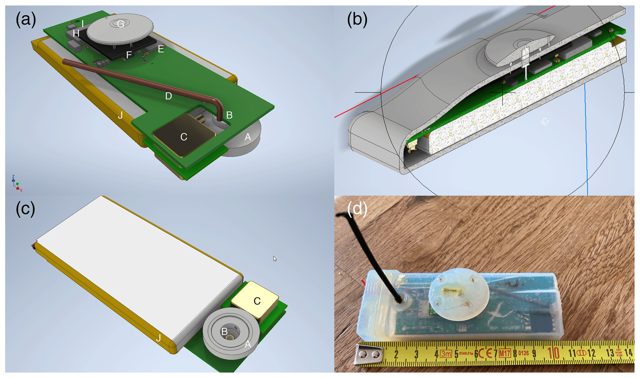
Figure 13D CAD design of (a) the top of the PCB, (b) the casing, (c) the bottom of the PCB with pressure dome, and (d) a picture of the actual platform. The PCB hosts: a pressure dome (a-A/c-A), a barometric pressure sensor (a-B/c-B), a differential pressure sensor (a-C/c-C), a PEEKsil red series capillary (a-D), an accelerometer (a-F), an anemometer (a-F) with the heating element (a-G), a microcontroller (a-H), a GPS (a-I), and a lithium battery (a-J/c-J).
The communication between the microcontroller and MEMS sensor on the PCB is either done by inter-integrated circuit (I2C) or serial peripheral interface (SPI) and depends on the sensor and personal preference. Both communication methods are bus protocols and allow for serial data transfer. However, SPI handles full-duplex communication, simultaneous communication between the microcontroller and MEMS sensor, while I2C is half-duplex. Therefore, I2C has the option of clock stretching, and the communication is stopped whenever the MEMS sensor cannot send data. In addition, I2C has built-in features to verify the data communication (e.g., start/stop bit, acknowledgement of data). Although the I2C protocol is favorable, it requires more power.
The microcontroller runs on self-made software, complementing the required manufacturers electrical and communication protocols. The software allows one to determine the sample time, sample frequency, and data storage. The PCB includes a 64 MB flash memory, which is used to store the data. The raw output of the digital MEMS sensors are stored as bits and the microcontroller performs no data processing to save power consumption. To extract data, the platform needs to be connected to a computer. There are no wireless communication possibilities.
2.2 Casing design for pressure measurements
The mobile sensor platform is designed to measure atmospheric parameters. Hence, a waterproof casing has been created using a Formlabs SLA 3D printer (Formlabs, 2020) to protect the PCB. Because of the use of a durable resin, the casing is waterproof and airtight. At the bottom of the casing, a dome structure is integrated (Fig. 1c), which acts as an inlet to both the absolute and differential pressure sensors. Note that the dome is not connected to the inside of the casing. The inlets of both sensors and a capillary are integrated within the dome designs and sealed with silicone glue, avoiding water and air leakage. Moreover, a Gore-Tex air-vent sticker (Gore-Tex, 2020) is used to cover the dome, which allows airflow but restrains water and salt in measurements near or above the ocean.
Air turbulence can generate dynamic pressure effects or stagnation pressure at the pressure dome (Raspet et al., 2019). The stagnation pressure increases with altitude, which results in higher wind speeds. Atmospheric measurements at altitude might therefore be influenced by stagnation pressure (Bowman and Lees, 2015; Smink et al., 2019; Krishnamoorthy et al., 2020). The influence of stagnation pressure on pressure measurements is theoretically elucidated by Raspet et al. (2008).
The application of a quad-disk might remove the stagnation pressure. Quad-disks are developed to cancel dynamic pressure effects and help detect slower static pressure changes or acoustic perturbations. Theoretical analysis of the quad-disk indicates that it should remove sufficient dynamic pressure to be useful for turbulence studies (Wyngaard and Kosovic, 1994). However, recent studies have shown a minimum effect of quad-disks on infrasound recordings (Krishnamoorthy et al., 2020). The casing of the INFRA-EAR is designed and developed for mobile and rapid deployments at remote places; adding a quad-disk to the design will expand the dimensions of the casing. Moreover, the pressure dome is positioned at the bottom of the casing, not oriented towards the dominant wind direction, in order to minimize the stagnation pressure on the pressure sensors.
Furthermore, within this design, the casings volume acts as a backing volume for the differential pressure sensor. One inlet of the differential pressure sensor is attached to the outside (via the dome) while the casing encloses the other inlet. A PEEKsil red series capillary is attached to the outside of the casing, ensuring pressure leakage between the backing volume and the atmosphere.
2.3 GPS
For measuring geophysical parameters on a high-resolution temporal scale, it is crucial to know the position and time of the measurement at high precision. To maintain knowledge regarding the position, a GNS2301 GPS is mounted on the PCB (Texim Europe, 2013). The GPS has a spatial accuracy of ±2.5 m up to 20 km altitude.
Besides providing an accurate position, the GPS also prevents drifting of the microcontroller's internal clock under the influence of, for example, weather. The time root mean square jitter, the deviation between GPS and actual time, is ±30 ns.
3.1 Infrasound sensor
The human audible sound spectrum is approximately between 20 and 20 000 Hz. Frequencies below 20 Hz or above 20 kHz are referred to as infrasound and ultrasound, respectively. The movement of large air volumes generates infrasound signals with amplitudes in the range of millipascals to tens of pascals. Examples of infrasound sources include earthquakes, lightning, meteors, nuclear explosions, interfering oceanic waves, and surf (Campus and Christie, 2010). Detection of infrasound depends on the signal's strength relative to the noise levels at a remote sensor (array), i.e., the signal-to-noise ratio. The signal strength depends, in turn, on the transmission loss that a signal experiences while propagating from source to receiver (Waxler and Assink, 2019). Local wind noise conditions predominantly determine the noise (Raspet et al., 2019) in addition to the sensor self-noise. Due to the presence of atmospheric waveguides and low absorption at infrasonic frequency (Sutherland and Bass, 2004), infrasonic signals can be detected at long distances from an infrasonic source. It is assumed that the source levels are sufficiently high so that the long-range signal is above the ambient noise conditions on the receiver side and the sensor is sensitive enough to detect the signal.
The infrasonic wavefield is conventionally measured with pressure transducers since such scalar measurements are relatively easy to perform. Those measurements can either be performed by absolute or differential pressure sensors. An absolute pressure sensor consists of a sealed aneroid and a measuring cavity connected to the atmosphere. A pressure difference within the measuring cavity will deflect the aneroid capsule. The mechanical deflection is converted to a voltage (Haak and De Wilde, 1996). The measurement principle of a differential infrasound sensor relies on the deflection of a compliant diaphragm, which is mounted on a cavity inside the sensor. The membrane deflects due to a pressure difference inside and outside the microphone, which occurs when a sound wave passes. A pressure equalization vent is part of the design to make the microphone insensitive to slowly varying pressure differences originating from long-period changes in weather conditions (Ponceau and Bosca, 2010).
Acoustic particle velocity sensors constitute a fundamentally different class of sensors that measure the airflow over sets of heated wires. This information quantifies the 3D particle velocity at one location, since the measurement is carried out in three directions (De Bree, 2003; Evers and Haak, 2000). Although such sensors' design is more involved and the sensors are far more costly, these sensors do allow for the measurement of sound directivity at one position, besides just the loudness.
Various studies show sensor self-noise and sensitivity curves of infrasound sensors (Ponceau and Bosca, 2010; Merchant, 2015; Slad and Merchant, 2016; Marty, 2019; Nief et al., 2019). The IMS specifications state that the sensor self-noise should be at least 18 dB below the global low-noise curves at 1 Hz (Brown et al., 2014), generated from global infrasound measurements using the IMS. Typical infrasound sensor networks, such as the IMS, use analogue sensors connected to a separate data logger to convert the measured voltage differences to a digital signal. The sensor's characteristic sensitivity determines the sensor resolution, i.e., the smallest difference that the sensor can detect. The resolution of the built-in analogue-to-digital (ADC) converters and the digitizing voltage range determine the data logger's resolution. Current state-of-the-art data loggers have a 24-bit resolution. New infrasound sensor techniques involve digital outputs since the ADC conversion is realized inside the sensor (Nief et al., 2017, 2019).
3.1.1 Sensor design
In this section, the mobile digital infrasound sensor's design is discussed, the KNMI mini-microbarometer (mini-MB). The design of this instrument is based on the following requirements. The sensor should have a flat, linear response over a wide infrasonic frequency band, e.g., 0.05–10 Hz. The sensor should be sensitive to the range of pressure perturbations in this frequency band, which are in the range of millipascals to tens of pascals. Moreover, the sensor and logging components' self-noise should be below the ambient noise levels of the IMS (Brown et al., 2014). Taking this into account, the sensor must also be low-cost (i.e., tens of dollars), small in dimensions (i.e., millimeter), and have a low energy consumption (i.e., milliampere).
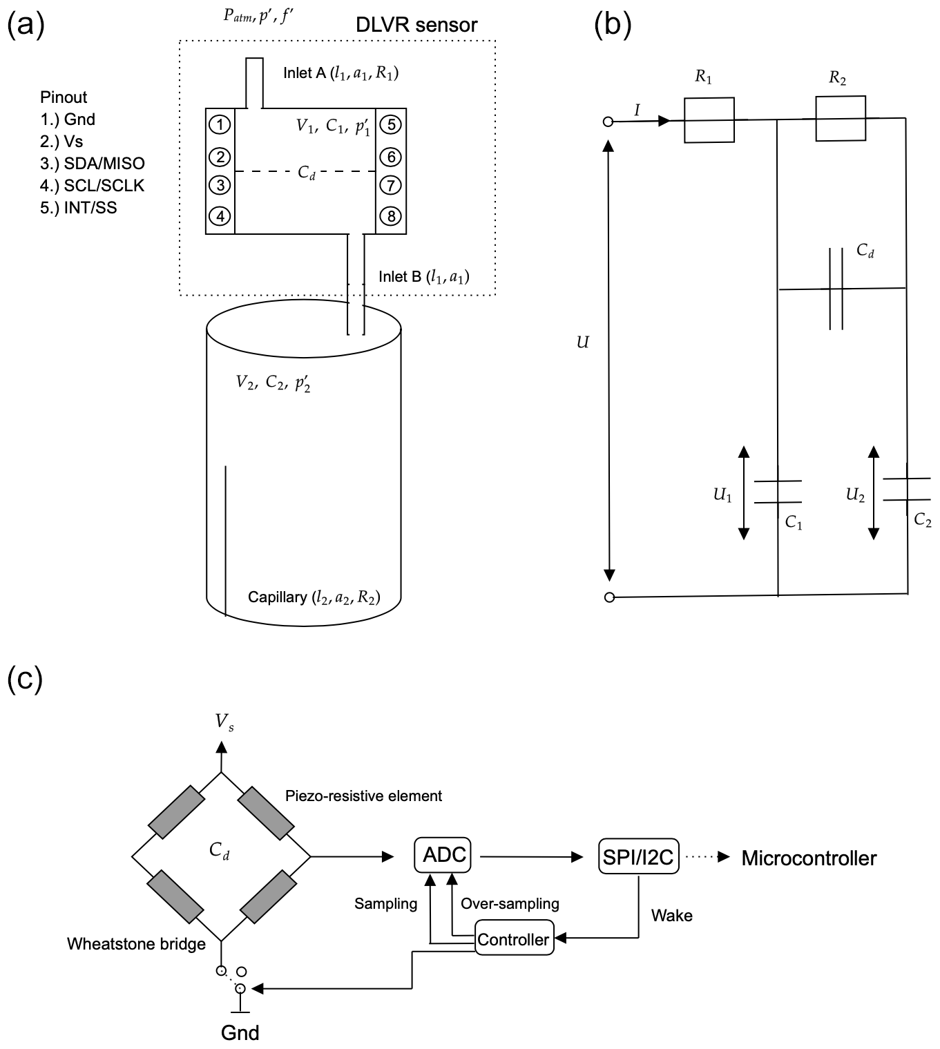
Figure 2The KNMI mini-MB design with the DLVR sensor and the parameters as listed in Table 1 (a) and the electrical circuit of the mini-MB (b). Panel (c) visualizes the DLVR sensor.
In this study, infrasound is measured with a differential pressure sensor. The measurement principle relies on the deflection of a diaphragm, which is mounted between two inlets. One inlet is connected to the atmosphere while the other is connected to a cavity (Fig. 2). The digital MEMS DLVR-F50D differential pressure sensor from All Sensors Inc. (DLVR, 2019) is used as a sensing element within the mini-MB. This sensor has a 16.5 mm × 13.0 mm × 7.3 mm dimension and has a linear response between ±125 Pa with a maximum error band of ±0.7 Pa. A Wheatstone bridge senses the diaphragm's deflection by measuring the changes in the piezo-resistive elements attached to the diaphragm. The sensor's output is an analogue voltage, which is subsequently digitized by the built-in 14-bit ADC, offering a maximum resolution of 0.02 Pa per count.
3.1.2 Theoretical response
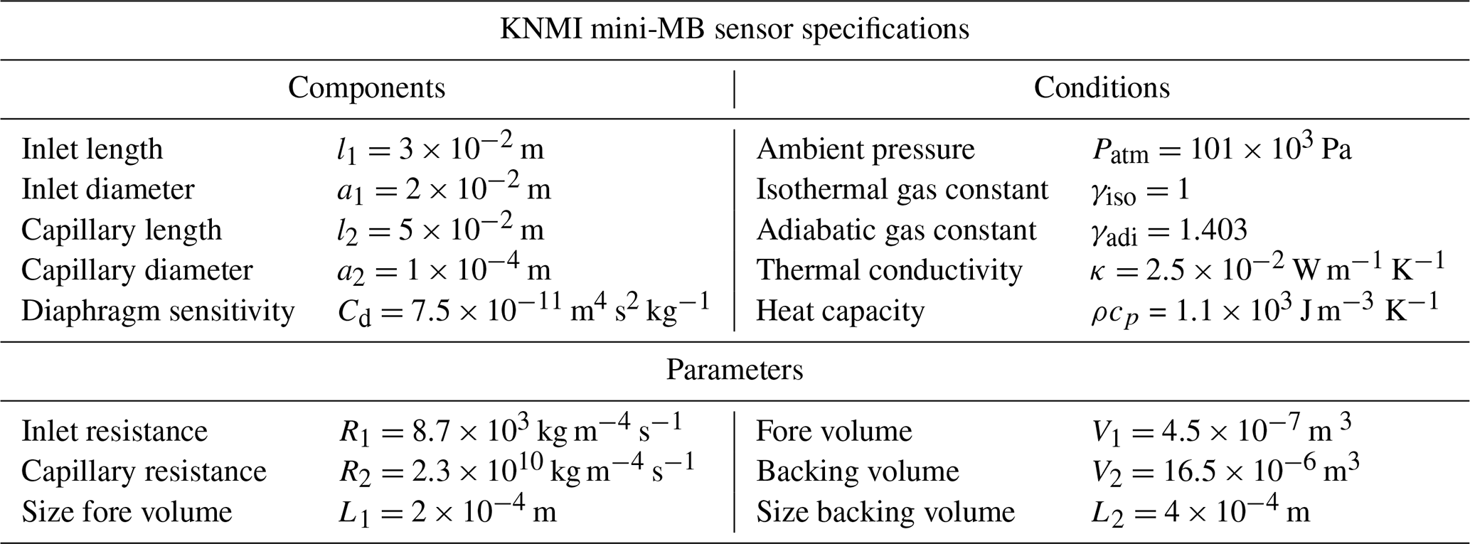
To measure differential pressure, the atmosphere is sampled through inlet A, which has a low resistance (R1), and is connected to a small fore volume (V1). Inlet B is connected to a backing volume (V2), which is connected to the atmosphere by capillary that acts as a high acoustic resistance (R2), which determines the low-frequency cutoff. Due to an external pressure wave, an observed pressure difference between the two inlets occurs and causes a deflection of the membrane (Cd) (Fig. 2a).
A theoretical response D(iω) for a differential pressure sensor as function of the angular frequency ω(=2πf) has been derived by Mentink and Evers (2011) following Burridge (1971):
where
Patm indicates the ambient barometric pressure, and γ is the thermal conduction of air. τj represent the time constants and depend on R1 and R2, which are the resistances of the inlet and capillary, and C1 and C2, the capacities of the fore and backing volume.
Figure 2a represents the sensor setup from an acoustical perspective, where Fig. 2b represents the electrical analogues of the sensor. The acoustical pressure difference () and volume flux (f′) are interpreted as an electrical voltage and current (I). The equivalent of the electrical resistance (R) corresponds to the ratio between acoustical pressure and the volume flux, whereas the capacitance (C) relates to the ratio of volume and ambient barometric pressure. The diaphragm's mechanical sensitivity (Cd) is the ratio of volume change and pressure change (Zirpel et al., 1978).
From an analysis of Eq. (1), it follows that inlet A dominates in the high-frequency limit. Hence, indicates the high-frequency cutoff of the sensor:
While at low frequencies, it is obtained that frequencies much smaller than are averaged out. Therefore the low-frequency limit can be determined as
which is controlled by the characteristics of the capillary, R2, and the size of the backing volume, V2. The acoustical resistance of the inlet R1 and the capillary R2 is described using Poiseuille's law (Washburn, 1921), which couples the resistance of airflow through a pipe (i.e., an inlet or capillary) to its length lj and diameter aj, by
where η stands for the viscosity of air, which equals 18.27 µPa s at 18 ∘C. Combining Eqs. (5) and (6) results in the theoretical low-frequency cutoff:
Besides the high and low ends of the response, it is of interest to determine the sensor response behavior within the passband ().
The three contributions in the denominator influence the passband behavior of the sensor:
-
A broadband frequency response depends on a constant pressure within the reference volume over the frequencies of interest (i.e., τ1≪τ2).
-
The pressure difference at the diaphragm is determined by the relative acoustical resistances connected to the sensor. The stability of the sensor response is assured by the capillary's large resistance because of which R1≪R2.
-
The sensor response depends on the ratio between the volumetric displacement of the diaphragm (Cd) versus the reference volume (C2). For the mini-MB, this term can be neglected.
Figure 3 shows the theoretical sensor frequency response for amplitude (Fig. 3a) and phase (Fig. 3b) for isothermal (red) and adiabatic (blue) behavior. The transitional behavior of the sensor response between isothermal and adiabatic behavior will be discussed in the next section.
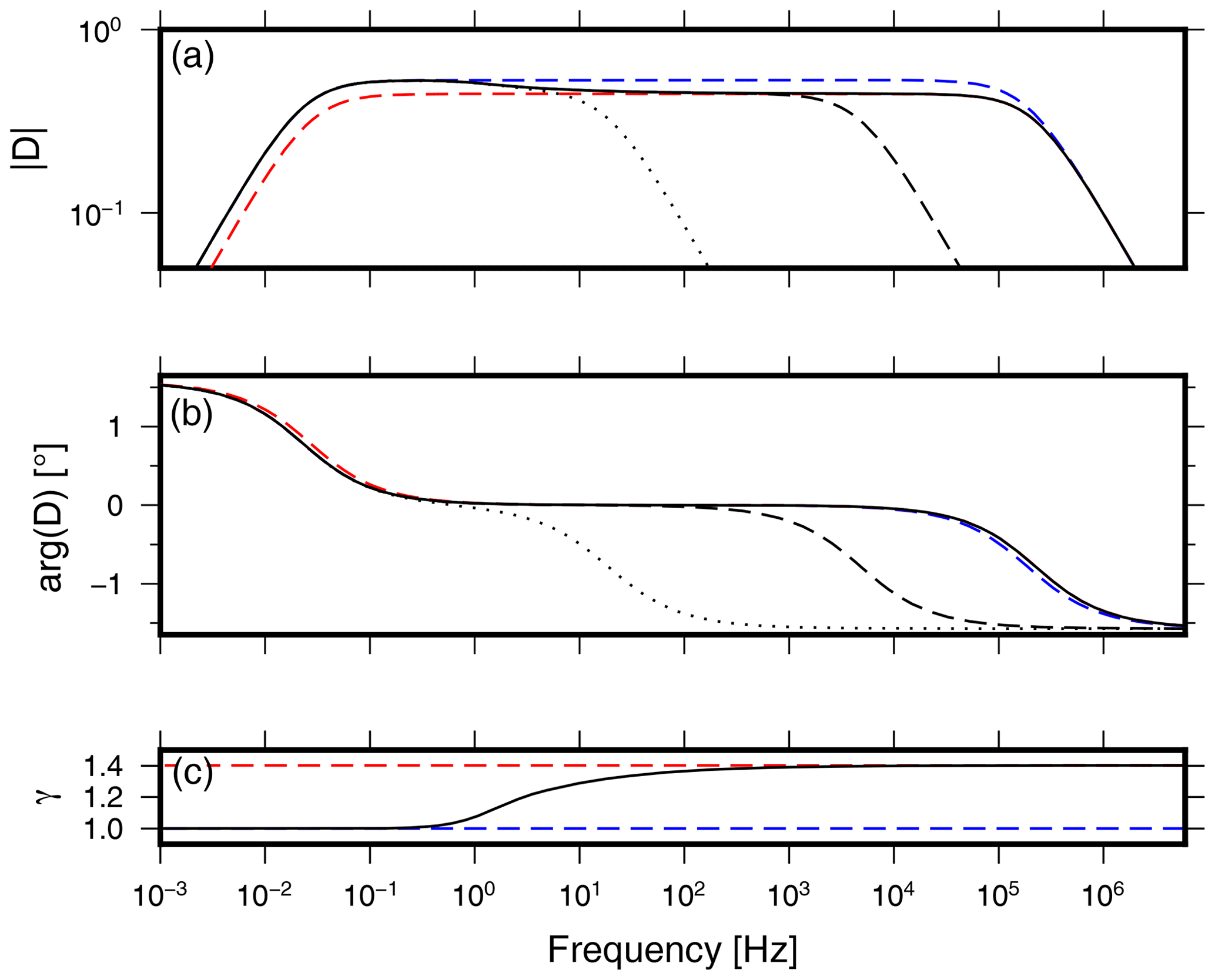
Figure 3The theoretical sensor frequency response function for (a) amplitude and (b) phase in the case of isothermal and adiabatic gas behavior in blue and red, respectively. The solid black line indicates the corrected sensor response by (c), as discussed in Sect. 3.1.3. The dotted and dashed lines indicate the high-frequency shifting cutoff due to Rgore, as discussed in Sect. 3.1.4.
3.1.3 Adiabatic–isothermal transition
Due to the presence of heat conduction within the sensor, air's compressive behavior is neither isothermal nor adiabatic. Instead, a transition from isothermal to adiabatic behavior is expected in the infrasonic frequency band (Richiardone, 1993; Mentink and Evers, 2011). In the transition zone, the heat capacity ratio can be effectively described by
where Λ indicates the correction factor to the heat capacity ratio γ. A difference in Λ will influence the capacitance values of the fore and backing volumes (Eq. 3).
Whether a sound wave in an enclosure behaves isothermally or adiabatically depends on the size of the thermal penetration depth δt relative to characteristic length L of the enclosure. L is defined as the ratio between the enclosure's volume and surface, i.e., . The thermal penetration depth is specified as the gas layer thickness in which heat can diffuse through during the time of one wave period and is derived as , where indicates the thermal diffusivity, defined as the ratio of thermal conductivity (κ) and heat capacity per unit volume (ρcp). Adiabatic gas behavior is obtained when and isothermal gas behavior when . The correction factor Λ is a function of and is thus frequency dependent; it can be derived as
where
x and y represent the real and imaginary components of a complex-valued function , which is dependent on the geometrical shape of the enclosure and the thermal penetration depth. In between the adiabatic and isothermal limits, the correction factor Λ describes the transition from an adiabatic heat ratio (i.e., γ=1.4) to an isothermal heat ratio, i.e., γ=1. The transition frequency defines the point where the maximum correction of Λ occurs, i.e., for which , from which follows that .
In the case of the mini-MB, the fore and backing volume have different shapes and sizes. The backing volume can be described as a long cylinder, L2, whereas the fore volume has a rectangular shape, L1. According to those geometries, the transition frequency of the fore and backing volume are 0.5 and 2.2 Hz, respectively. Since and the sensor response above is adiabatic, while the response below is isothermal. Therefore, the thermal conduction correction's main effect is found to be in the passband region (Eq. 8).
The mini-MB has been designed to have a broadband response; therefore, only the third term of the dominator is influenced by the correction factor. The effect of thermal conduction to the response is due to ratio , which means that the correction factor is characterized by the geometric component of the backing volume:
where Z indicates the characteristic correction assuming a long cylinder (Mentink and Evers, 2011). indicates the ratio of L to δt, while J0 and J1 are the zeroth- and first-order Bessel functions of the first kind.
The corrected theoretical sensor response is obtained by substituting . Figure 3c shows the value of in the transaction zone between isothermal and adiabatic gas behavior. The black line in Fig. 3a and b indicates the corrected theoretical sensor response.
In the case of the mini-MB, the isothermal-to-adiabatic transition results in an effect on the amplitude of % and on the phase of less than a degree. Note that implies that the backing volume is relatively large such that the change in gas behavior does not influence the sensitivity of the diaphragm.
3.1.4 Gore-Tex air vent
As discussed in Sect. 3.1.2., the high- and low-frequency cutoff are controlled by the resistivity of the inlet and backing volume, respectively. A Gore-Tex V9 sticker is added to the opening of the casing's pressure dome, which changes the resistivity of the inlets. The Gore-Tex V9 vent allows an airflow of m3 s−1 m−2. Poiseuille's second law, Eq. (6), shows the airflow resistivity caused by an open pipe and can be rewritten as
where Δp indicates the pressure difference between both sides of the pipe and qv the volumetric airflow.
Table 1KNMI mini-MB components, parameter values, and standard conditions used in the computations.
For the differential pressures that the mini-MB sensor is able to sense, ranging from 0.02 to 125 Pa, with a Gore-Tex air-vent area of m2, the equivalent resistivity Rgore ranges from 5×10⁵ to 3.125×10⁸ kg m−4 s−1. Comparing the resistivity of the air vent with the resistivity values of the capillary and the inlet of the sensor, Table 1 shows that the air vent will only influence the inlet's resistivity. Assuming the vent behaves linearly, the high-frequency cutoff of the sensor decreases to a value of around 15 Hz. Figure 3 shows the theoretical transfer function for the mini-MB with a Gore-Tex air vent attached to the inlet. The high-frequency cutoff shifts between the dotted line and the dashed line due to varying values of Rgore.
3.1.5 Experimental response
The theoretical sensor response describes the high- and low-frequency cutoff. Eq. (7) and the parameters listed in Table 1 show that the mini-MB has a theoretical low-frequency cutoff of 0.042 Hz. A sudden over- or under-pressure (i.e., impulse response) is applied to the sensor to determine the low-frequency cutoff experimentally (Evers and Haak, 2000). The impulse forces the diaphragm out of equilibrium. The capillary and the size of the backing volume control the time to return into equilibrium again. The time it takes for the diaphragm to reach equilibrium again corresponds to a characteristic relaxation time proportional to the low-frequency cutoff.
The outcome of the experimental low-frequency cutoff was determined to be 0.044±0.0025 Hz. The theoretical low-frequency cutoff falls within the error margins of the experimental cutoff frequency. The small difference between both is assumed to be due to experimental errors in timing the relaxation time as well as small imperfections in the used capillary (Evers, 2008). It follows from Eq. (6) that the low-frequency cutoff is inversely proportional to the radius to the fourth power. Hence, a 1 % deviation in the capillary radius will lead to a 4 % deviation in low-frequency cutoff.
3.1.6 Sensor self-noise
The resolution, the smallest change detectable by a sensor, depends on the sensor measurement range and the number of ADC bits. Having a linear response over a pressure range of ±125 Pa and a 14-bit built-in ADC results in a 0.02 Pa per count resolution. Besides the ADC resolution, the accuracy of the measurement depends on the sensor's internal error, the self-noise. The self-noise corresponds to the diaphragm's deformation caused by the mass of the diaphragm plus the electrical noise from the digitizer. As it is a digital sensor, it is impossible to follow the conventional methods to determine self-noise (Sleeman et al., 2006). Therefore the self-noise is determined by opening both inlets to a closed pressure chamber, ensuring no pressure difference between them. The outcome stated that the self-noise falls within the sensor's maximum error band, ±0.7 Pa (DLVR, 2019). Since no backing volume is used, and the cavities at both sides of the diaphragm are small, the relation changes (Eq. 8). Due to this, it is necessary to correct the sensor response for the adiabatic-to-isothermal transition. (Sect. 3.1.3).
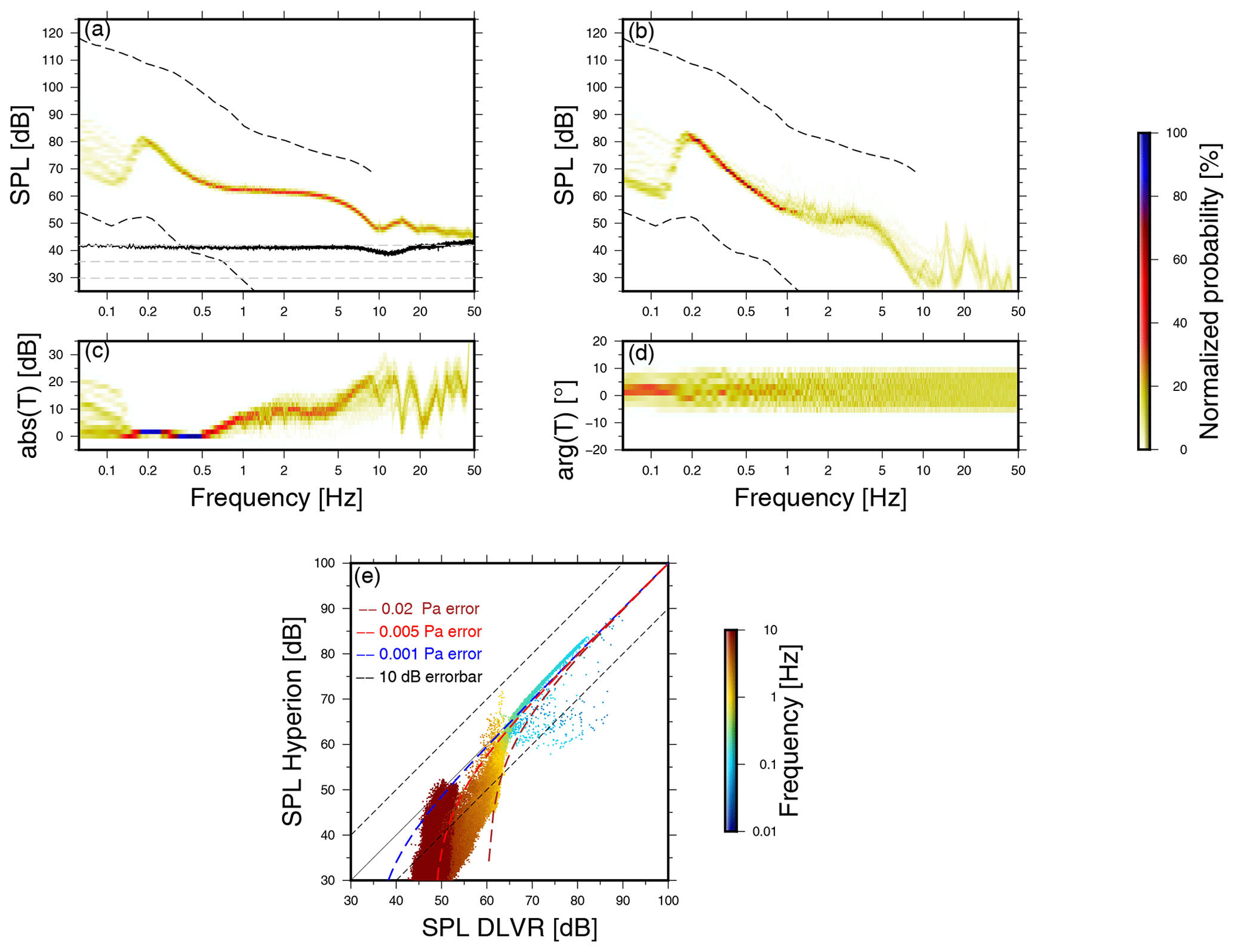
Figure 4PDFs of pressure spectra recorded with the mini-MB (a) and the Hyperion sensor (b) for a week of continuous recording in dB re 20−6 Pa2 Hz−1. The dashed lines indicate the infrasonic high and low ambient noise levels (Brown et al., 2014). Panel (a) shows the PSD of the 24 h self-noise recording of the mini-MB in black and the theoretical self-noise for a 12-, 13-, and 14-bit ADC as the gray dashed lines. Panels (c) and (d) visualize the absolute difference T in amplitude and phase between the mini-MB and the Hyperion as a function of frequency. Panel (e) displays the differences in sound pressure level measured by the mini-MB and the Hyperion sensor for the various frequencies.
The self-noise consistency is determined by calculating the power spectral density (PSD) curves for each hour over a test period of 24 h (Merchant and Hart, 2011). Figure 4a shows in black the average 90th percentile confidence interval of the self-noise. Note that the instrumental self-noise exceeds the global low-noise model (Brown et al., 2014) at frequencies above 0.4 Hz. Compared to high-fidelity equipment that typically falls entirely below the global low-noise models, such self-noise levels are relatively high, yet comparable to levels attained by similar sensor designs (Marcillo et al., 2012). Furthermore, note that the self-noise follows the dynamic range of a 12-bit ADC, as indicated by the gray dotted line (Sleeman et al., 2006). The sensor has a maximum “no missing code” of 12 bits, the effective number of bits (DLVR, 2019).
3.1.7 Sensor comparison
A comparison between the mini-MB and a Hyperion IFS-5111 sensor (Merchant, 2015) is made to assess the mini-MB performance relative to the reference Hyperion sensor. Both sensors have been placed inside a cabin next to the outside sensor test facility at the leading author's institute. There is a connection to the outside pressure field through air holes in the wall of the cabin. The Hyperion sensor has been configured with a high-frequency shroud. Figure 4a and b show the Probability Density Function (PDF) (Merchant and Hart, 2011) of the data recorded by the mini-MB and the Hyperion sensor, respectively. Both sensors resolved the characteristic microbarom peak around 0.2 Hz (Christie and Campus, 2010). The spectral peaks above 10 Hz correspond to resonances that exist inside the measurement shelter.
A direct comparison of the pressure recordings are shown in Fig. 4c, d, and e. Figure 2c shows the absolute difference in amplitude over frequency, where panel d indicates the phase difference between both sensors. Panel (e) shows the relative difference between the mini-MB and the Hyperion sensor. The sensors are in good agreement over the passband frequencies. A larger deviation is shown for the low-end (f<0.07 Hz) and high-end frequencies(f>8 Hz). At frequencies between 0.07 and 1 Hz, the pressure values are positively biased by 5 ± 1 dB, which equals a measurement error by the KNMI mini-MB of ±0.005 Pa (Fig. 4e). Above 1 Hz, the pressure values are biased by 10 ± 5 dB, which equals a measurement error of ±0.02 Pa.
The backing volume causes a deviation in the low-frequency spectrum. The high-frequency deviation is due to the relatively high noise level of the mini-MB. For the higher frequencies, the mini-MB PDF follows the 12-bit dynamic range. Only in the case of significant events or loud ambient noise, can the sensor sense pressure perturbations in the high-frequency range. Nonetheless, the mini-MB falls within a 30 dB error range over the entire frequency band compared to the Hyperion IFS-5111 sensor.
3.2 Meteorological parameters
The detectability of infrasound is directly linked to wind noise conditions and the atmosphere's stability in the infrasound sensor's surroundings since noise levels are increased when turbulence levels are high. Therefore, it is beneficial to have simultaneous measurements of the basic meteorological parameters, i.e., pressure, wind, and temperature. The sub-sections below describe the different meteorological measurements contained on the sensor platform.
3.2.1 Barometric pressure sensor
The barometric pressure is sensed by the LPS33HW sensor (STMicroelectronics, 2017), which is part of the pressure dome. Similarly to the differential pressure sensor, piezo-resistive crystals measure the barometric pressure.
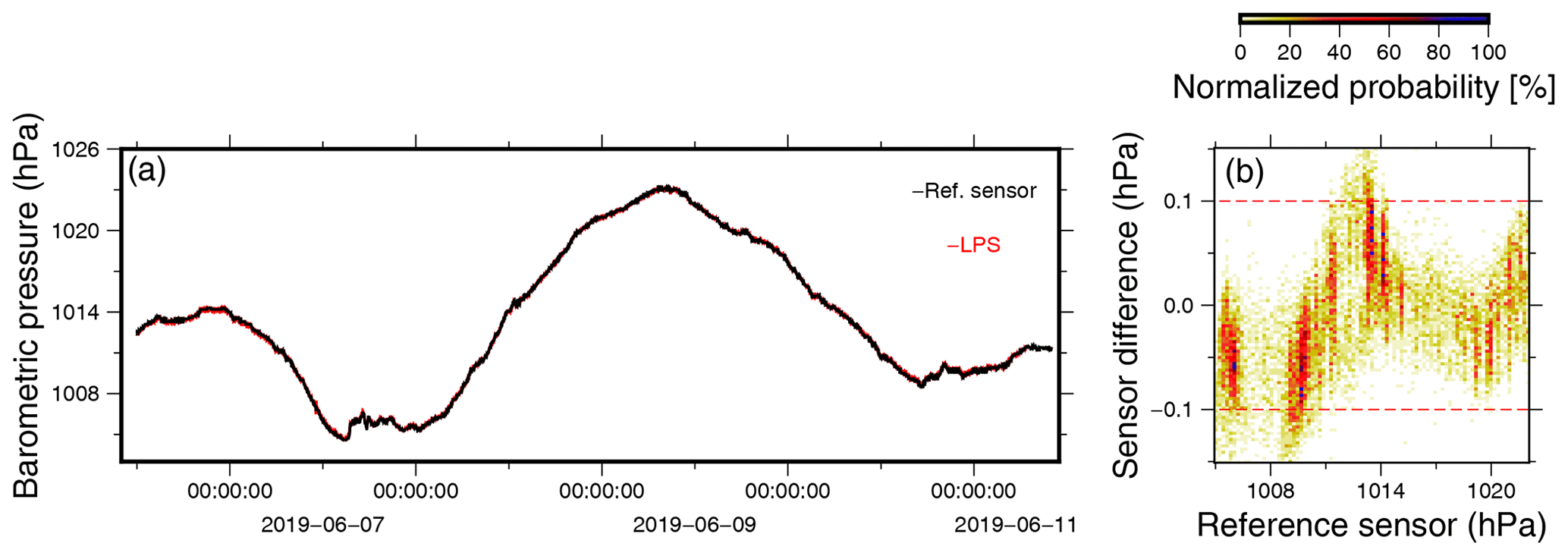
Figure 5A comparison between the barometric MEMS sensor (red) and a KNMI reference barometer (black). Panel (a) shows 5 d of barometric pressure recordings using both sensors, while panel (b) displays the difference in measured barometric pressure by the MEMS and the reference sensor.
Calibration tests are performed within a pressure chamber in which a cycle of static pressures between 960 and 1070 hPa can be produced. Besides the MEMS sensor, the chamber is equipped with a reference sensor. This procedure resulted in a calibration curve, which describes the pressure-dependent systematic bias. After correcting for the bias, the LPS sensor has an accuracy of ±0.1 hPa, i.e., the LPS sensors measure values within ± 0.1 hPa of the value measured by the KNMI reference sensor. Furthermore, the LPS sensor has been field-tested (Fig. 5a), along with a Paroscientific Digiquartz 1015A barometer, which has an accuracy of 0.05 hPa. From the distribution of observations, it can be estimated that the LPS sensor has a precision of ±0.1 hPa for 93 % of the time (Fig. 5b). For the remainder, the maximum deviation was ±0.15 hPa.
3.2.2 Wind sensor
In addition to coherent acoustic signals, the pressure field at infrasonic frequencies consists to a large degree of pressure perturbations due to wind and turbulence (Walker and Hedlin, 2010). This turbulent energy is present over the complete infrasonic frequency range with a typical noise amplitude level decrease with increasing frequencies, following a slope (Raspet et al., 2019).
To reduce wind turbulence interference with the acoustic perturbations, a wind-noise reduction system (WNRS) can be put in place (Walker and Hedlin, 2010; Raspet et al., 2019). Most WNRSs consist of a non-porous pipe rosette, with low impedance inlets at each pipe's end. All pipes are connected to four main pipes, which connect to the microbarometer. By doing so, the atmosphere is sampled over a larger area and thus small incoherent pressure perturbations (e.g., wind) are filtered out.
The sensor presented in this paper is designed for mobile sampling campaigns. In such cases, the application of similar WNRS filters cannot be attained. Not having a WNRS decreases the SNR; measuring wind with an anemometer will give an insight into the wind conditions. Therefore, simultaneous measurement of wind and infrasound provides better insight into the infrasonic SNR conditions.
Sensor design
A 2D omnidirectional heat mass flow sensor has been designed to measure the wind conditions, which is a robust and passive anemometer (Fig. 6a). The sensor is built with a central heating element, which heats to approximately 80 ∘C, and is circularly surrounded by six TDK thermistors (TDK, 2018). Depending on the wind direction and speed, the temperature field around the center element is modified. The wind speed and direction can be estimated from the 2D temperature gradient, i.e., its absolute value and direction.
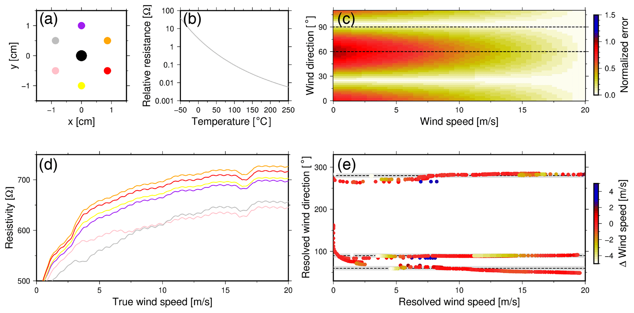
Figure 6Analyses of the anemometer. Panel (a) shows the top view of the sensor design, with the central heating element. Panel (b) indicates the resistivity of the thermistors over temperature. The geometric sensitivity for the anemometer is shown in panel (c). The thermistors' measured resistance for calibration setup 2 (90∘), for which the colors are in agreement with the sensor design (a), are shown in panel (d). Panel (e) indicates the resolved wind direction and wind speed compared with the actual direction (dotted lines) and correct wind speed of setups 1 (270∘), 2 (90∘), and 3 (60∘). The gray shaded area indicates the ±5∘ accuracy interval.
Theoretical response
The six sensing elements are placed within a distance of 1 cm from the heating element, while two thermistors and the heating element are at a spatial angle of 60∘. The thermistors measure the temperature gradient caused by the wind flow since the resistance is strongly sensitive to temperature. The thermistors are made of semiconductor material and have a negative temperature coefficient. The resistance decreases non-linearly with increasing temperature. The Steinhart–Hart equation approximately describes the temperature T as a function of resistance value RΩ (Steinhart and Hart, 1968):
where , , and are the thermistor constants received by the manufacturer (TDK, 2018). However, they can as well be determined by taking three calibration measurements, for which the temperature and resistance are known, and solving the three equations simultaneously. Figure 6b shows the sensitivity curve for the TDK thermistor. The thermistor has a relative value of 1Ω at 25 ∘C and a precision of ±4 % ∘C−1, which leads to a 0.05 ∘C error. This error value is placed in context by modeling the expected temperate difference under representative meteorological conditions in the next section.
Numerical sensor response
The heating element needs to transfer a minimum temperature difference around the sensing elements (i.e., the sensing elements error). A numerical model has been built in ANSYS (ANSYS, 2018) to define the amount of temperature difference around the sensing elements under different meteorological circumstances. The model is a first approximation of the sensitivity and is based on homogeneous laminar airflow passing by the sensor. Turbulent flow along the anemometer, caused by the sensor design or casing, generates uncertainties within the measurements.
This first approximation of sensitivity follows a numerical forward modeling technique to approximate the heat probe's shape and intensity at a sensing element. The model was run at stable meteorological parameters (i.e., 8 ∘C air temperature, 50 % humidity, and 10 m s−1 wind speed). The outcome shows that under those circumstances, the sensing element experiences a temperature difference of around 4 ∘C. Together with the outcome of the thermistors' sensitivity curve, it is concluded that the designed sensor can resolve this airflow and is used to estimate wind speed and direction.
Conversion of sensor output into atmospheric parameters
To convert the measured resistivity into atmospheric parameters, a 2D planar temperature gradient has been estimated numerically from the discrete set of measurements. The measurement resistivities have been transformed into temperature measurements following Eq. (14). Based on those temperatures, a 2D numerical temperature gradient has been reconstructed. The problem is analogous to the estimation of the wavefront directivity from travel time differences (Szuberla and Olson, 2004).
In the present case, there are N=6 discrete sample points, each with an coordinate and a temperature value Tj. The total differential of the temperature describes the variation of temperature T(x,y) as a function of x and y:
From Eq.(15), it follows that we can determine the 2D gradient by setting up a system of N equations. In this case, the number of unknowns is two, and thus the gradient could be estimated by two measurements. However, in practice, errors are introduced due to measurement errors. Therefore the set of equations becomes inconsistent, which leads to nonsensical solutions. The unknown set of parameters is solved by over-determining the system in a least-squares sense to overcome this problem. Equation (15) can be rewritten in terms of a matrix–vector system:
where y represents the temperature difference between two measurement points, matrix X represents the pairwise separations, and p represents the temperature gradient ∇T. It is assumed that the measurement errors ϵ can be described by a normal distribution, i.e., a random variable with mean E(ϵ)=0 and variance Var(ϵ)=σ2. It can be been shown that the least-squares estimate of p, here labeled , can be obtained by solving the following equation:
where † represents the transpose operator. The solution satisfies Eq. (16) with the constraint that the sum of squared errors is minimized. The matrix X and the error term ϵ determine the solution's accuracy. If a Gaussian distribution can represent the measurement errors, it can be shown that the least-squares solution is unbiased.
Based on the 2D reconstruction of the temperature gradient (Eq. 18), the wind direction and speed is resolved with an estimated accuracy. Furthermore, this method allows determining the uncertainty based on geometric sensor setup (Szuberla and Olson, 2004). Figure 6c shows the least-squares error analyses of the sensor design (Fig. 6a). It stands out that the uncertainty increases when one element is positioned close to the wind flow (i.e., at 60∘).
Reference calibration
Experimental calibration of the anemometer has been performed at the KNMI calibration lab. The calibration lab features a wind tunnel, which generates a laminar airflow ranging between 0–20 m s−1. Within the wind tunnel, two mechanical anemometers are installed, which serve as reference sensors. With its MEMS anemometer, the mobile platform is installed right below one of the reference sensors to ensure that the mobile platform does not obstruct the laminar flow in the tunnel.
The calibration procedure consists of multiple independent calibration tests that will be described next. First, the sensor is placed inside the wind tunnel while there is no airflow. This way, the relative difference between the sensing elements is determined, the so-called zero measurement. The sensor is corrected for the internal bias by correcting for the relative difference, which varies around ±25 ohm. After correcting the sensor bias, the sensor is placed within the horizontal plane (i.e., with a pitch angle of 0∘) at different angles concerning the airflow. For every angle, the flow speed is varied between 0 and 20 m s−1.
The calibration shows that the measured resistance of the thermistors increases with increasing wind speeds. High wind speeds increasingly cool down the thermistors, resulting in higher resistances. Figure 6d shows the six thermistors' measured resistance over the actual wind speed.
The wind direction and the accuracy of the anemometers have been determined according to Eq. (17). Three different sensor setups show the accuracy and precision over increasing wind speeds as a function of directivity. The outcome of calibration setups 1 (270∘), 2 (90∘), and 3 (60∘) are shown, respectively, in Fig. 6e. The mean direction over all wind speeds, for the three setups, is 89, 272, and 57∘. The standard deviation shows that the sensor's accuracy is ±5∘. Furthermore, it is shown that the precision of the wind direction increases with increasing wind speeds. The resolved wind speeds by the anemometer and the difference with the correct wind speed are shown in Fig. 6e. The colors indicate the difference between resolved wind speed and correct wind speed within the wind tunnel. The mean deviation between resolved and correct wind speed is ±2 m s−1. Again, it is shown that the accuracy increases with increasing wind speeds.
3.3 Accelerometer
The sensing element of the infrasound sensor on this platform is a sensitive diaphragm. Strong accelerations of the platform will cause a deflection of the diaphragm and may obscure infrasonic signal levels. In addition, such accelerations may be misinterpreted as infrasound if no independent accelerometer information is available. To be able to separate the mechanical response of the sensor from actual signals of interest, the platform measures accelerations for which the LSM303, a 6-axis inertial measurement unit (IMU), is deployed (STMicroelectronics, 2018). The LSM303 consists of a 3-axis accelerometer and 3-axis magnetometer. The measurement range of the accelerometer varies between approximately 2–16 g. The magnetometer is out of the scope of this study and therefore neglected.
Accelerometers measure differential movement between the gravitational field vector and its reference frame. In the absence of linear acceleration, the sensor measures the rotated gravitational field vector, which can be used to calibrate the sensor. A rotational movement of the sensor will result in acceleration. The IMU is a digital sensor with a built-in 16-bit ADC and has a resolution of 0.06 mg when choosing the lowest measurement range.
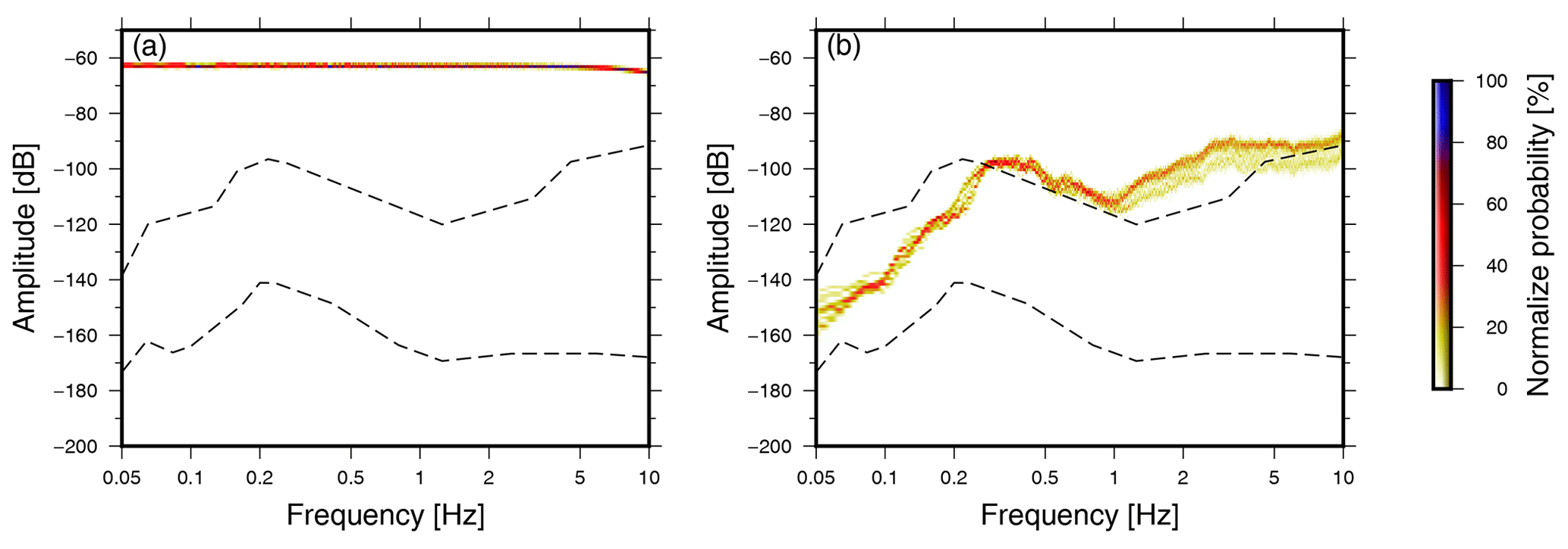
A comparison test has been carried out in the seismic pavilion of the author's institute. Inside this pavilion, the LSM is compared to a Streckeisen STS-2 seismometer connected to a Quanterra Q330 as a reference sensor (KNMI, 1993). Both sensors are installed on pillars to ensure a good coupling between the subsurface and the sensor. The comparison test, which is based on 24 h of recording, shows that the accuracy of the LSM303 3-axis accelerometer is ±1.5 mg (1.5 cm s−2). Figure 7 shows the PDFs of the comparison test for the MEMS and STS-2 sensor. While the sensors are deployed on the same seismic pillar and are thus subject to similar seismic noise conditions, the MEMS sensor could not measure ambient seismic noise (Peterson, 1993; McNamara and Buland, 2004) due to its high self-noise level. The LSM accelerometer exceeds both the U.S. Geological Survey New High Noise Model (NHNM) (Peterson, 1993) and the STS-2 reference sensor by at least 35 dB.
It is therefore unlikely to use this IMU for monitoring purposes of ambient seismic noise or teleseismic events. Previous studies drew similar conclusions concerning the performance of MEMS accelerometers. Various calibration setups are considered while comparing MEMS accelerometers with conventional accelerometers of geophones (Hons et al., 2008; Albarbar et al., 2009; Anthony et al., 2019), each concluding that the accuracy of the MEMS is not sufficient for recording ambient seismic noise. However, during strong local events or boisterous environments the MEMS sensor will resolve those seismic signals.
In this study, the constructional efforts and calibration protocols of the INFRA-EAR are presented. The INFRA-EAR is a low-cost mobile multidisciplinary sensor platform for the monitoring of geophysical quantities. It includes sensors for the measurement of infrasound, acceleration, barometric pressure, and wind.
The platform uses the newest sensor technology, i.e., digital MEMS, which have a built-in ADC. The MSP430 programmable microcontroller unit controls the sampling of the ADC and the storage of the data samples. A MEMS GPS is a unit to determine the positioning and to prevent clock drift. Due to the small dimensions of MEMS and their low energy consumption, the “infrasound logger” is a pocket-size measurement platform, powered by an 1800 mAh lithium battery. The platform does not require any infrastructure (e.g., data connection, power supply, and specific mounting) as commonly used for the deployment of high-fidelity systems, which makes it mobile and allows rapid deployments and measurements at remote places.
The INFRA-EAR is specifically designed to measure infrasound. The platform hosts the KNMI mini-MB, a novel design with a pressure dome as inlet, the casing as backing volume with a PEEKsil capillary, and the DLVR-F50D as the sensing element. The low-frequency cutoff of mini-MB depends on the size of the backing volume, and the capillary characteristics. The high-frequency cutoff depends on the mini-MB inlet parameters, which is partly controlled by a Gore-Tex air vent (Sect. 3.1.4). The infrasound logger has a low-frequency cutoff frequency of 0.044±0.0025 Hz, while the high-frequency cutoff varies between 15 and 90 Hz.
A comparison between the mini-MB and a Hyperion infrasound sensor (Merchant, 2015) has shown the differences in amplitude and phase (Fig. 4). The mini-MB has an amplitude difference of 30 dB for the passband frequencies band compared to the Hyperion sensor. The sensors are in good agreement for the lower frequencies and both sensors resolved the characteristic microbarom peak around 0.2 Hz (Christie and Campus, 2010). However, the higher frequencies show small deviations, which is due to the relatively high noise band of the mini-MB. From 8 Hz onward, the mini-MB PDF follows the 12-bit dynamic range of the ADC. Nonetheless, the mini-MB can resolve the infrasonic ambient noise field up to ±8 Hz. Only in the case of significant events or boisterous conditions, can the sensor sense pressure perturbations in the higher frequency range.
When the wind-noise levels are high, infrasound signals can be masked and remain undetected. Therefore, the sensor platform presents a passive anemometer to give insights into the wind conditions during infrasonic measurements. The MEMS anemometer is built up as an omnidirectional sensor. Numerical tests indicate that the temperature difference caused by a wind flow around the thermistors should be significant to be sensed. For validation, the anemometer has been calibrated inside a wind tunnel. Figure 6 shows the outcome of the calibration tests. Based on this outcome, one can conclude that the anemometer can determine wind direction and wind speed given that the sensor is calibrated. The sensor measures a difference in resistance, which is converted into a temperature measurement. The discreet temperature measurements are used to reconstruct a 2D planar temperature gradient, which is used to determine the wind speed and direction. Based on the calibration tests within the wind tunnel, it is shown that the anemometer has a directional accuracy of ±5∘ and a wind speed accuracy of ±2 m s−1. Nonetheless, it is shown in Fig. 6c that the anemometer has geometrical uncertainties due to it design. Future anemometers, 2D hot wire, should consider a minimum of eight thermistors to exclude geometric uncertainties (Szuberla and Olson, 2004).
Besides an anemometer and infrasound sensor, the platform also hosts a barometric pressure sensor, an accelerometer, and GPS. Each sensor has been calibrated and compared with a reference sensor. It was shown that the accelerometer has a relatively high self-noise, which restricts the sensors ability to determine the ambient seismic noise (Peterson, 1993; McNamara and Buland, 2004). Nonetheless, the sensor will most likely resolve local transient events, which influences the mini-MB's sensitivity and its ability to resolve infrasonic sources. The barometric sensor shows good agreement with a reference sensor (Fig. 5). Absolute pressure perturbations due to the weather are resolved. After calibration, the sensor has a precision of ±0.1 hPa for 93 % of the time. For the remainder, the maximum deviation was ±0.15 hPa compared to the reference sensor.
Calibration tests performed in this study and previously show that the MEMS sensors perform less than the commonly used high-fidelity sensors. The self-noise of the sensors is a critical problem. Furthermore, the MEMS sensors manufacturers highlight a significant change of measurement drift (DLVR, 2019; TDK, 2018; STMicroelectronics, 2017, 2018); regular calibration is needed. Nonetheless, the MEMS sensor techniques are continuously developing (Manjiyani et al., 2014; Johari, 2003). The INFRA-EAR design is such that the platform can be adjusted and improved by adding or swapping sensors. Mobile sensor platforms, built up by PCBs and digital MEMS sensors, are therefore scalable, flexible, and ready for various geophysical measurements.
Nonetheless, a low-cost mobile multidisciplinary sensor platform can complement existing high-fidelity geophysical sensor networks. This study showed that as long as the MEMS are well-calibrated, they perform in agreement with the reference sensors. Therefore, the INFRA-EAR can contribute significantly to providing observations during remote or rapid deployments (e.g., weather towers, weather balloons, and scientific balloons) to complement the existing sensor network by increasing observations. Although the sensor data do not fully satisfy the measurement requirements, the improvement of spatial resolution enables stacking the observations. This can be realized by stacking the output of various sensor platforms or adding more sensors to the same sensor platform and averaging the output (Nishimura et al., 2019). Stacking improves the signal-to-noise ratio by , where N is the number of observations.
Initially, the INFRA-EAR was designed as a biologger for the monitoring of atmospheric parameters. In total, 25 INFRA-EARs were produced and used during the 2020 field campaign at the Crozet Islands in the Southern Ocean. The loggers were fitted to the Southern Ocean's largest seabirds, the Wandering Albatross (Diomedea exulans). The Southern Hemisphere has very few in situ measurements due to limited shore areas. The use of INFRA-EAR in such areas is ideal for monitoring geophysical parameters, comparing in situ measurements, and comparing INFRA-EAR data with model data.
The software and design of the sensor platform are available upon request from Dominique Filippi.
The data of the reference sensors are available at FDSN webservices: https://doi.org/10.21944/e970fd34-23b9-3411-b366-e4f72877d2c5 (KNMI, 1993). Soon the data of the sensor platform will also be accessible on FDSN.
OFCdO has lead the study, design, development, calibration, test, analysis, and manuscript. JDA and LGE have consulted during the entire study and contributed to refining the manuscript text. CDO and DF have consulted and helped designing and developing the platform.
The authors declare that they have no conflict of interest.
The authors thank the calibration lab of the KNMI for their collaboration, explanation of the different calibration techniques, and permission to perform experimental tests at their facility. Furthermore, the authors would like to thank Sam Patrick, Mathieu Basille, Susana Clusella-Trullas, Thomas Clay, Rocio Joo, and Jeff Zeyl for their input regarding selecting the used MEMS sensors. All figures have been created using Generic Mapping Tools (Wessel et al., 2013). The manuscript is a guide for the design, development, and calibration of multidisciplinary sensor platforms. Based on the manuscript, sensor platforms can either be self-produced or ordered from Dominique Filippi (co-author) of Sextant Technology, Inc.
This research has been supported by the Human Frontier Science Program Young Investigator Grant (SeabirdSound, grant no. RGY0072/2017) and a VIDI project from the Dutch Research Council (NWO, project no. 864.14.005).
This paper was edited by Andreas Zahn and reviewed by two anonymous referees.
Albarbar, A., Badri, A., Sinha, J. K., and Starr, A.: Performance evaluation of MEMS accelerometers, Measurement, 42, 790–795, 2009. a
Anderson, J. F., Johnson, J. B., Bowman, D. C., and Ronan, T. J.: The Gem infrasound logger and custom-built instrumentation, Seismol. Res. Lett., 89, 153–164, 2018. a, b
ANSYS: ANSYS Academic Research Mechanical, Release 18.1, available at: https://www.ansys.com/academic/terms-and-conditions (last access: 16 February 2021), 2018. a
Anthony, R. E., Ringler, A. T., Wilson, D. C., and Wolin, E.: Do low-cost seismographs perform well enough for your network? An overview of laboratory tests and field observations of the OSOP Raspberry Shake 4D, Seismol. Res. Lett., 90, 219–228, 2019. a
Assink, J., Averbuch, G., Shani-Kadmiel, S., Smets, P., and Evers, L.: A seismo-acoustic analysis of the 2017 North Korean nuclear test, Seismol. Res. Lett., 89, 2025–2033, 2018. a
Averbuch, G., Assink, J. D., and Evers, L. G.: Long-range atmospheric infrasound propagation from subsurface sources, J. Acoust. Soc. Am., 147, 1264–1274, 2020. a
Blanc, E., Ceranna L., Hauchecorne, A., Charlton-Perez, A., Marchetti, E., Evers, L. G., Kvaerna, T., Lastovicka, J., Eliasson, L., Crosby, N. B., Blanc-Benon, P., Le Pichon, A., Brachet, N., Pilger, C., Keckhut, P., Assink, J. D., Smets, P. S. M., Lee, C. F., Kero. J., Sinderlarova, T., Kampfer, N., Rufenacht, R., Farges, T., Millet, C., Nasholm, S. P., Gibbons, S. J., Espy, P. J., Hibbins, R. E., Heinrich, P., Ripepe, M., Khaykin, S., Mze, N., and Chum, J.: Toward an improved representation of middle atmospheric dynamics thanks to the ARISE project, Surv. Geophys., 39, 171–225, 2018. a
Bowman, D. C. and Lees, J. M.: Infrasound in the middle stratosphere measured with a free-flying acoustic array, Geophys. Res. Lett., 42, 10010–10017, 2015. a
Brown, D., Ceranna, L., Prior, M., Mialle, P., and Le Bras, R. J.: The IDC seismic, hydroacoustic and infrasound global low and high noise models, Pure Appl. Geophys., 171, 361–375, 2014. a, b, c, d
Burridge, R.: The acoustics of pipe arrays, Geophys. J. Int., 26, 53–69, 1971. a
Campus, P. and Christie, D.: Worldwide observations of infrasonic waves, in: Infrasound monitoring for atmospheric studies, Springer, Dordrecht, the Netherlands, 185–234, 2010. a
Christie, D. and Campus, P.: The IMS infrasound network: Design and establishment of infrasound stations, in: Infrasound monitoring for atmospheric studies, Springer, Dordrecht, the Netherlands, 29–75, 2010. a, b
Cornes, R. C., Dirksen, M., and Sluiter, R.: Correcting citizen-science air temperature measurements across the Netherlands for short wave radiation bias, Meteorol. Appl., 27, e1814, https://doi.org/10.1007/978-1-4020-9508-5_2, 2020. a
D'Alessandro, A., Luzio, D., and D'Anna, G.: Urban MEMS based seismic network for post-earthquakes rapid disaster assessment, Adv. Geosci., 40, 1–9, https://doi.org/10.5194/adgeo-40-1-2014, 2014. a, b
De Bree, H.-E.: The Microflown: An acoustic particle velocity sensor, Acoust. Aust., 31, 91–94, 2003. a
DLVR: Technical Report DLVR Series Low Voltage Digital Pressure Sensors, available at: https://www.allsensors.com/datasheets/DS-0300_Rev_E.pdf (last access: 16 February 2021), 2019. a, b, c, d
Evers, L. G.: The inaudible symphony: on the detection and source identification of atmospheric infrasound, PhD thesis, TU Delft, Delft University of Technology, Delft, the Netherlands, 2008. a, b
Evers, L. G. and Haak, H. W.: The Deelen Infrasound Array: on the detection and identification of infrasound, Internal report, Royal Netherlands Meteorological Institute (KNMI), De Bilt, the Netherlands, 2000. a, b
Fang, Z., Zhao, Z., Du, L., Zhang, J., Pang, C., and Geng, D.: A new portable micro weather station, in: 2010 IEEE 5th International Conference on Nano/Micro Engineered and Molecular Systems, 20–23 January 2010, Xiamen, China, IEEE, 379–382, 2010. a
Formlabs: Technical Report Formlabs 3D printer, Formlabs, available at: https://media.formlabs.com/m/1aa00d88fe52d5bc/original/-ENUS-Form-3B-Manual.pdf (last access: 16 February 2021), 2020. a
Garcia-Marti, I., de Haij, M., Noteboom, J. W., van der Schrier, G., and de Valk, C.: Using volunteered weather observations to explore urban and regional weather patterns in the Netherlands, AGU Fall Meeting Abstracts, 9–13 December 2019, San Fransico, CA, USA, IN22A–08, 2019. a
Gore-Tex: Technical Report Gore TEX air vents, Gore-Tex, available at: https://www.gore.com/products/gore-protective-vents-for-other-outdoor-applications (last access: 16 February 2021), 2020. a
Grangeon, J. and Lesage, P.: A robust, low-cost and well-calibrated infrasound sensor for volcano monitoring, J. Volcanol. Geoth. Res., 387, 106668, https://doi.org/10.1016/j.jvolgeores.2019.106668, 2019. a
Green, D., Matoza, R., Vergoz, J., and Le Pichon, A.: Infrasonic propagation from the 2010 Eyjafjallajökull eruption: Investigating the influence of stratospheric solar tides, J. Geophys. Res.-Atmos., 117, D21202, https://doi.org/10.1029/2012JD017988, 2012. a
Grimmett, D., Plate, R., and Goad, J.: Measuring Infrasound from the Maritime Environment, in: Infrasound Monitoring for Atmospheric Studies, Springer, Cham, Switzerland, 173–206, 2019. a
Haak, H. W. and De Wilde, G.: Microbarograph systems for the infrasonic detection of nuclear explosions, Royal Netherlands Meteorological Institute (KNMI), De Bilt, the Netherlands, 1996. a
Homeijer, B., Lazaroff, D., Milligan, D., Alley, R., Wu, J., Szepesi, M., Bicknell, B., Zhang, Z., Walmsley, R., and Hartwell, P.: Hewlett packard's seismic grade MEMS accelerometer, in: 2011 IEEE 24th International Conference on Micro Electro Mechanical Systems, 23–27 January 2011, Cancun, Mexico, IEEE, 585–588, 2011. a
Homeijer, B. D., Milligan, D. J., and Hutt, C. R.: A brief test of the hewlett-packard mems seismic accelerometer, US Geological Survey Open-file Report, https://doi.org/10.3133/ofr20141047, 2014. a
Hons, M., Stewart, R., Lawton, D., Bertram, M., and Hauer, G.: Field data comparisons of MEMS accelerometers and analog geophones, The Leading Edge, 27, 896–903, 2008. a
Huang, Q.-A., Qin, M., Zhang, Z., Zhou, M., Gu, L., Zhu, H., Hu, D., Hu, Z., Xu, G., and Liu, Z.: Weather station on a chip, in: SENSORS, 22–24 October 2003, Toronto, ON, Canada, IEEE, vol. 2, 1106–1113, 2003. a
Johari, H.: Development of MEMS sensors for measurements of pressure, relative humidity, and temperature, PhD thesis, Worcester Polytechnic Institute, available at: http://citeseerx.ist.psu.edu/viewdoc/download?doi=10.1.1.594.7980&rep=rep1&type=pdf (last access: 16 February 2021), 2003. a
KNMI: Netherlands Seismic and Acoustic Network, Royal Netherlands Meteorological Institute (KNMI), Other/Seismic Network [data set], https://doi.org/10.21944/e970fd34-23b9-3411-b366-e4f72877d2c5, 1993. a, b
Krishnamoorthy, S., Bowman, D. C., Komjathy, A., Pauken, M. T., and Cutts, J. A.: Origin and mitigation of wind noise on balloon-borne infrasound microbarometers, J. Acoust. Soc. Am., 148, 2361–2370, 2020. a, b
Laine, J. and Mougenot, D.: Benefits of MEMS based seismic accelerometers for oil exploration, in: TRANSDUCERS 2007–2007 International Solid-State Sensors, Actuators and Microsystems Conference, 10–14 June 2007, Lyon, France, IEEE, 1473–1477, https://doi.org/10.1109/SENSOR.2007.4300423, 2007. a, b
Lammel, G.: The future of MEMS sensors in our connected world, in: 2015 28th IEEE International Conference on Micro Electro Mechanical Systems (MEMS), 18–22 January 2015, Estoril, Portugal, IEEE, 61–64, https://doi.org/10.1109/MEMSYS.2015.7050886, 2015. a
Ma, R.-H., Wang, Y.-H., and Lee, C.-Y.: Wireless remote weather monitoring system based on MEMS technologies, Sensors, 11, 2715–2727, 2011. a
Manjiyani, Z. A. A., Jacob, R. T., Keerthan Kumar, R., and Varghese, B.: Development of MEMS based 3-axis accelerometer for hand movement monitoring, International Journal of Computer Science and Engineering Communications, 2, 87–92, 2014. a
Manobianco, J. and Short, D. A.: On the Utility of Airborne MEMS for Improving Meteorological Analysis and Forecasting, in: 2001 International Conference on Modeling and Simulation of Microsystems, 19–21 March 2001, Hilton Head Island, SC, USA, 342–345, 2001. a
Marcillo, O., Johnson, J. B., and Hart, D.: Implementation, characterization, and evaluation of an inexpensive low-power low-noise infrasound sensor based on a micromachined differential pressure transducer and a mechanical filter, J. Atmos. Ocean. Tech., 29, 1275–1284, 2012. a, b, c, d
Marty, J.: The IMS infrasound network: current status and technological developments, in: Infrasound Monitoring for Atmospheric Studies, Springer, 3–62, https://doi.org/10.1007/978-3-319-75140-5_1, 2019. a, b
McNamara, D. E. and Buland, R. P.: Ambient noise levels in the continental United States, B. Seismol. Soc. Am., 94, 1517–1527, 2004. a, b
Mentink, J. H. and Evers, L. G.: Frequency response and design parameters for differential microbarometers, J. Acoust. Soc. Am., 130, 33–41, 2011. a, b, c
Merchant, B. J.: Hyperion 5113/GP infrasound sensor evaluation, Sandia Report SAND2015–7075, Sandia National Laboratories, Albuquerque, New Mexico, USA, 2015. a, b, c
Merchant, B. J. and Hart, D. M.: Component evaluation testing and analysis algorithms, Technical Report No. SAND2011-8265, Sandia National Laboratories, Albuquerque, New Mexico, USA, 2011. a, b
Milligan, D. J., Homeijer, B. D., and Walmsley, R. G.: An ultra-low noise MEMS accelerometer for seismic imaging, in: SENSORS, 28–31 October 2011, Limerick, Ireland, IEEE, 1281–1284, https://doi.org/10.1109/ICSENS.2011.6127185, 2011. a
Nief, G., Olivier, N., Olivier, S., and Hue, A.: New Optical Microbarometer, in: AGU Fall Meeting Abstracts, 11–15 December 2017, New Orleans, Louisiana, USA, vol. 2017, A21A–2150, 2017. a
Nief, G., Talmadge, C., Rothman, J., and Gabrielson, T.: New generations of infrasound sensors: technological developments and calibration, in: Infrasound Monitoring for Atmospheric Studies, Springer, 63–89, https://doi.org/10.1007/978-3-319-75140-5_2, 2019. a, b
Nishimura, R., Cui, Z., and Suzuki, Y.: Portable infrasound monitoring device with multiple MEMS pressure sensors, in: International Congress on Acoustics (ICA), 3–9 September 2019, Aachen, Germany, 1498–1505, 2019. a
Peterson, J. R.: Observations and modeling of seismic background noise, Tech. rep., US Geological Survey, available at: http://opg.sscc.ru/attachments/073_ofr93-322.pdf (last access: 16 February 2021), 1993. a, b, c, d
Poler, G., Garcia, R. F., Bowman, D. C., and Martire, L.: Infrasound and Gravity Waves Over the Andes Observed by a Pressure Sensor on Board a Stratospheric Balloon, J. Geophys. Res.-Atmos., 125, e2019JD031565, https://doi.org/10.1029/2019JD031565, 2020. a
Ponceau, D. and Bosca, L.: Low-noise broadband microbarometers, in: Infrasound monitoring for atmospheric studies, Springer, 119–140, https://doi.org/10.1007/978-1-4020-9508-5_4, 2010. a, b
Raspet, R., Yu, J., and Webster, J.: Low frequency wind noise contributions in measurement microphones, J. Acoust. Soc. Am., 123, 1260–1269, 2008. a
Raspet, R., Abbott, J.-P., Webster, J., Yu, J., Talmadge, C., Alberts II, K., Collier, S., and Noble, J.: New systems for wind noise reduction for infrasonic measurements, in: Infrasound Monitoring for Atmospheric Studies, Springer, 91–124, https://doi.org/10.1007/978-3-319-75140-5_3, 2019. a, b, c, d
RBOOM: Specifications for: Raspberry Boom (RBOOM) and “Shake and Boom” (RS&BOOM), available at: https://manual.raspberryshake.org/_downloads/SpecificationsforBoom_SnB.pdf (last access: 16 February 2021), 2017. a
Richiardone, R.: The transfer function of a differential microbarometer, J. Atmos. Ocean. Tech., 10, 624–628, 1993. a
Shani-Kadmiel, S., Assink, J. D., Smets, P. S., and Evers, L. G.: Seismoacoustic coupled signals from earthquakes in central Italy: Epicentral and secondary sources of infrasound, Geophys. Res. Lett., 45, 427–435, 2018. a
Slad, G. W. and Merchant, B. J.: Chaparral Model 60 infrasound sensor evaluation, Technical Report, Sandia report, SAND2016–1902, Sandia National Laboratories, Albuquerque, New Mexico, USA, 2016. a
Sleeman, R., Van Wettum, A., and Trampert, J.: Three-channel correlation analysis: A new technique to measure instrumental noise of digitizers and seismic sensors, B. Seismol. Soc. Am., 96, 258–271, 2006. a, b
Smink, M. M., Assink, J. D., Bosveld, F. C., Smets, P. S., and Evers, L. G.: A Three-Dimensional Array for the Study of Infrasound Propagation Through the Atmospheric Boundary Layer, J. Geophys. Res.-Atmos., 124, 9299–9313, 2019. a
Speller, K. E. and Yu, D.: A low-noise MEMS accelerometer for unattended ground sensor applications, in: Unattended/Unmanned Ground, Ocean, and Air Sensor Technologies and Applications VI, International Society for Optics and Photonics, vol. 5417, 63–72, https://doi.org/10.1117/12.540337, 2004. a
Steinhart, J. S. and Hart, S. R.: Calibration curves for thermistors, Deep sea research and oceanographic abstracts, 15, 497–503, https://doi.org/10.1016/0011-7471(68)90057-0, 1968. a
STMicroelectronics: Technical Report STMicroelectronics LPS33HW, STMicroelectronics, availabl at: https://www.st.com/resource/en/datasheet/lps33hw.pdf (last access: 16 February 2021), 2017. a, b
STMicroelectronics: Technical Report STMicroelectronics LSM303, STMicroelectronics, available at: https://www.st.com/resource/en/datasheet/lsm303agr.pdf (last access: 16 February 2021), 2018. a, b
Sutherland, L. C. and Bass, H. E.: Atmospheric absorption in the atmosphere up to 160 km, J. Acoust. Soc. Am., 115, 1012–1032, 2004. a
Szuberla, C. A. and Olson, J. V.: Uncertainties associated with parameter estimation in atmospheric infrasound arrays, J. Acoust. Soc. Am., 115, 253–258, 2004. a, b, c
TDK: Technical Report TDK NTC element G1540, TDK, available at: https://product.tdk.com/en/system/files?file=dam/doc/product/sensor/ntc/ntc_element/data_sheet/50/db/ntc/ntc_glass_enc_sensors_g1540.pdf (last access: 16 February 2021), 2018. a, b, c
Texim Europe: Technical Report Texim Europe GNS2301, Texim Europe, available at: http://static6.arrow.com/aropdfconversion/c1ea3946d7c9a03073e868dd440bd5fc6bce1506/19gns2301_datasheet.pdf.pdf(last access: 16 February 2021), 2013. a
Walker, K. T. and Hedlin, M. A.: A review of wind-noise reduction methodologies, in: Infrasound monitoring for atmospheric studies, Springer, 141–182, https://doi.org/10.1007/978-1-4020-9508-5_5, 2010. a, b
Washburn, E. W.: The dynamics of capillary flow, Phys. Rev., 17, 273, https://doi.org/10.1103/PhysRev.17.273, 1921. a
Waxler, R. and Assink, J.: Propagation modeling through realistic atmosphere and benchmarking, in: Infrasound Monitoring for Atmospheric Studies, Springer, 509–549, https://doi.org/10.1007/978-3-319-75140-5_15, 2019. a
Wessel, P., Smith, W. H., Scharroo, R., Luis, J., and Wobbe, F.: Generic mapping tools: improved version released, Eos, 94, 409–410, 2013. a
Wyngaard, J. and Kosovic, B.: Similarity of structure-function parameters in the stably stratified boundary layer, Bound.-Lay. Meteorol., 71, 277–296, 1994. a
Zirpel, M., Kraan, W., and Mastboom, P.-P.: Operationele versterkers: een verzameling schakelingen en formules voor de toepassing van operationele versterkers, Wolters Kluwer N.V., Alphen aan den Rijn, the Netherlands and Philadelphia, USA, 1978. a
Zou, X., Thiruvenkatanathan, P., and Seshia, A. A.: A seismic-grade resonant MEMS accelerometer, J. Microelectromech. S., 23, 768–770, 2014. a