Testing the altitude attribution and vertical resolution of AirCore measurements with a new spiking method

AirCore samplers have been increasingly used to capture vertical profiles of trace gases reaching from the ground up to about 30 km, in order to validate remote sensing instruments and to investigate transport processes in the stratosphere. When deployed to a weather balloon, accurately attributing the trace gas measurements to the sampling altitudes is nontrivial, especially in the stratosphere. In this paper we present the CO-spiking experiment, which can be deployed to any AirCore on any platform in order to evaluate different computational altitude attribution processes and to experimentally derive the vertical resolution of the profile by injecting small volumes of signal gas at predefined GPS altitudes during sampling. We performed two CO-spiking flights with an AirCore from the Goethe University Frankfurt (GUF) deployed to a weather balloon in Traînou, France, in June 2019. The altitude retrieval based on an instantaneous pressure equilibrium assumption slightly overestimates the sampling altitudes, especially at the top of the profiles. For these two flights our altitude attribution is accurate within 250 m below 20 km. Above 20 km the positive bias becomes larger and reaches up to 1.2 km at 27 km altitude. Differences in descent velocities are shown to have a major impact on the altitude attribution bias. We parameterize the time lag between the theoretically attributed altitude and the actual CO-spike release altitude for both flights together and use it to empirically correct our AirCore altitude retrieval. Regarding the corrected profiles, the altitude attribution is accurate within ±120 m throughout the profile. Further investigations are needed in order to test for the scope of validity of this correction parameter regarding different ambient conditions and maximum flight altitudes. We derive the vertical resolution from the CO spikes of both flights and compare it to the modeled vertical resolution. The modeled vertical resolution is too optimistic compared to the experimentally derived resolution throughout the profile, albeit agreeing within 220 m. All our findings derived from the two CO-spiking flights are strictly bound to the GUF AirCore dimensions. The newly introduced CO-spiking experiment can be used to test different combinations of AirCore configurations and platforms in future studies.

1 Introduction

The AirCore is a cost-effective atmospheric sampling technique originally developed by Tans (2009) and introduced by Karion et al. (2010) to capture vertical profiles of trace gases. In principle, it consists of a coiled stainless-steel tube that is sealed at one end and open at the other. During ascent, e.g., on a weather balloon, it empties due to the decreasing pressure with height, whereas during descent the surrounding air flows into the AirCore. After recovery the sample is analyzed for trace gas mole fractions with a continuous-flow gas analyzer and the resulting measurements are attributed to the sampling altitudes. AirCore samplers have been increasingly deployed to small weather balloons to capture continuous CO₂ and CH₄ profiles from the surface up to about 30 km at various locations around the world. Recently, AirCore measurements have been used to validate ground-based spectrometric data of the Total Carbon Column Observing Network (TCCON) (Sha et al., 2020; Tu et al., 2020), which is widely used to validate satellite data. Vertical information, which has been derived from ground-based remote sensing, has been compared with AirCore profiles (Karppinen et al., 2020; Zhou et al., 2019). Tadić and Biraud (2018) used AirCore data to evaluate their approach to estimate total column mole fractions of CO₂ and CH₄ using partial column data from aircraft flights. Further developments based on the AirCore sampling technique allow for new areas of application. For example, Andersen et al. (2018) developed an active AirCore sampling system and deployed it to a lightweight unmanned aerial vehicle for tropospheric sampling at locations that are difficult to access. Instead of passively sampling ambient air due to the increase in ambient pressure during descent, they used a pump to actively pull ambient air through their AirCore. Karion et al. (2010) proposed to deploy AirCore samplers to maneuverable gliders, which would facilitate probing specific air masses and recovering the AirCore. AirCore subsampling techniques have been developed that allow for analysis of isotopes (Mrozek et al., 2016; Paul et al., 2016) and halogenated trace gases with abundances well below 1 ppb (Laube et al., 2020). Stratospheric trace gas measurements play an important role in investigating dynamical changes in the stratosphere (Moore et al., 2014). Engel et al. (2017) derived the mean age of air at high altitudes from AirCore measurements in order to update their investigation of long-term changes in the overall overturning circulation of the stratosphere (Brewer–Dobson circulation) based on atmospheric observations presented in Engel et al. (2009). Their AirCore samplers were deployed to a large stratospheric balloon launched by CNES in 2015 and to small weather balloons flown in 2016.

The wide range of platforms and fields of application concerning AirCore sampling (regardless of being active or passive) all have one thing in common: a continuous sample of atmospheric air is collected together with meteorological and positional data, which need to be attributed to the trace gas measurements of the sample after analysis. Regarding vertical profiles from passive AirCore samplers, an altitude attribution approach has been suggested (Pieter Tans, NOAA, personal communication, 2020), which is based on modeling the pressure drop across the AirCore during sampling and the flow of air into the AirCore. However, until now a common approximation is to assume an instantaneous pressure equilibrium between the AirCore and ambient air and to use the ideal gas law to calculate the amount of sample for each time step during descent (e.g., Engel et al., 2017; Karion et al., 2010; Membrive et al., 2017). In addition, the start and end points of the AirCore in the continuous trace gas measurement time series need to be determined accurately, which relied on subjective judging until now (Engel et al., 2017; Membrive et al., 2017). The reliability of assuming an instantaneous pressure equilibrium during sampling for the altitude attribution depends on multiple factors (e.g., AirCore geometry, usage of a dryer, ascent and descent velocities, magnitude of pressure change with altitude). Due to the weak vertical pressure gradient at high altitudes, attributing the stratospheric part of balloon-based AirCore observations to the correct altitude is a challenging task, and it can be considered even more challenging when descent velocities are high. The latter is the case for descents that are decelerated solely by parachutes, which is the most common way for AirCore samplers flown from weather balloons. To our knowledge, the altitude attribution processes could only be validated by comparing AirCore profiles to in situ aircraft measurements and sampling flasks up to approximately 350 hPa (Karion et al., 2010) – corresponding to below 10 km – or comparison of different AirCore samplers on a slowly descending large stratospheric balloon (Engel et al., 2017; Membrive et al., 2017) or comparison with a lightweight stratospheric air sampler (Hooghiem et al., 2018), without quantifying any altitude attribution bias until now.

In this paper, we present a CO-spiking system, which is a newly developed technique that can be used in situ to evaluate any combination of AirCore, platform or altitude retrieval procedure. In principle, this technique could also be used to evaluate the positional retrieval of active AirCore samplers. Here, we focus on a passive AirCore that has been deployed to a weather balloon and on the commonly applied retrieval procedure that is based on assuming an instantaneous pressure equilibrium. In Sect. 2, we describe the AirCore and analytical setup, together with the retrieval procedure that we use and the technical CO-spiking setup. Two measurement flights that were conducted in Traînou, France, in June 2019 are presented in Sect. 3 together with the CO-spiking experiment results regarding altitude attribution, a possible correction parameter and the vertical resolution of the profiles at different altitudes. We summarize the findings of this paper and give conclusions in Sect. 4.

2 Experimental

2.1 Goethe University Frankfurt AirCore general approach

The Goethe University Frankfurt (GUF) AirCore sampler is designed to be lightweight and is thus allowed for use under small balloons at midlatitudes in Europe. Its geometry promotes a high sampling volume and reduces mixing due to diffusion during storage especially in the high-altitude sampling region, where tubing with a thinner inner diameter is used. The experimental setup, operation and data evaluation of the GUF AirCore have been published in detail in Engel et al. (2017).

Three thin-walled stainless-steel tubes with different diameters (internal diameters: 1.76, 3.6, 7.6 mm; outer diameters: 2, 4, 8 mm), coated with silconert2000^® and soldered together, result in the 100 m long and coiled GUF AirCore. This design allows for the rapid collection of air in the large-diameter tubing, which is then gradually pushed into the smaller-diameter tubing, where mixing by molecular diffusion is less effective. A dryer filled with Mg(ClO₄)₂ is connected to the inlet. The onboard electronic system that we used from 2019 on is based on the Arduino MEGA 2560 microcontroller. It comprises up to eight temperature sensors, a pressure sensor, a GPS antenna, an SD card holder for data logging. The microcontroller also controls the closing valve.

Before launch, the AirCore is flushed with fill gas (FG, air standard with known trace gas mole fractions) and sealed at one end. During ascent it empties due to the decreasing ambient pressure with height. A small amount of FG remains in the AirCore. During descent the AirCore fills with ambient air due to the increase in ambient pressure. Upon landing, the inlet is closed automatically. After retrieval the AirCore is brought back to the laboratory. The sample is pushed out of the AirCore with a push gas (PG) and analyzed with a Picarro G2401 CRDS (cavity ring-down spectrometer) continuous-flow gas analyzer for H₂O, CO, CH₄ and CO₂ mole fractions at a constant rate. FG and PG are identical in the GUF setup. Figure 1 shows the analytical setup for the measurement process. In the bypass or flushing position of the two-position valve (Fig. 1a), PG is measured and the open transfer lines to the AirCore are flushed. After connecting the AirCore to the transfer lines, the two-position valve is switched to measurement position (Fig. 1b) so that the sample is pushed through the analyzer. Since 17 June 2019, our Picarro analyzer operated in the inlet valve control mode at a constant rate at ∼ 30 cm³ min⁻¹ at standard temperature and pressure (STP, 1013 hPa, 0 ^∘C) for AirCore measurements. This is similar to previously published operating methods (e.g., Andersen et al., 2018; Membrive et al., 2017). The mass flow controller in the original measurement setup described in Engel et al. (2017) was replaced by a needle valve (NV) acting as a flow resistance close to the inlet of the Picarro analyzer. This setup has the advantage that the mass flow controller, which provides an additional source of mixing before the analysis cell, can be removed.

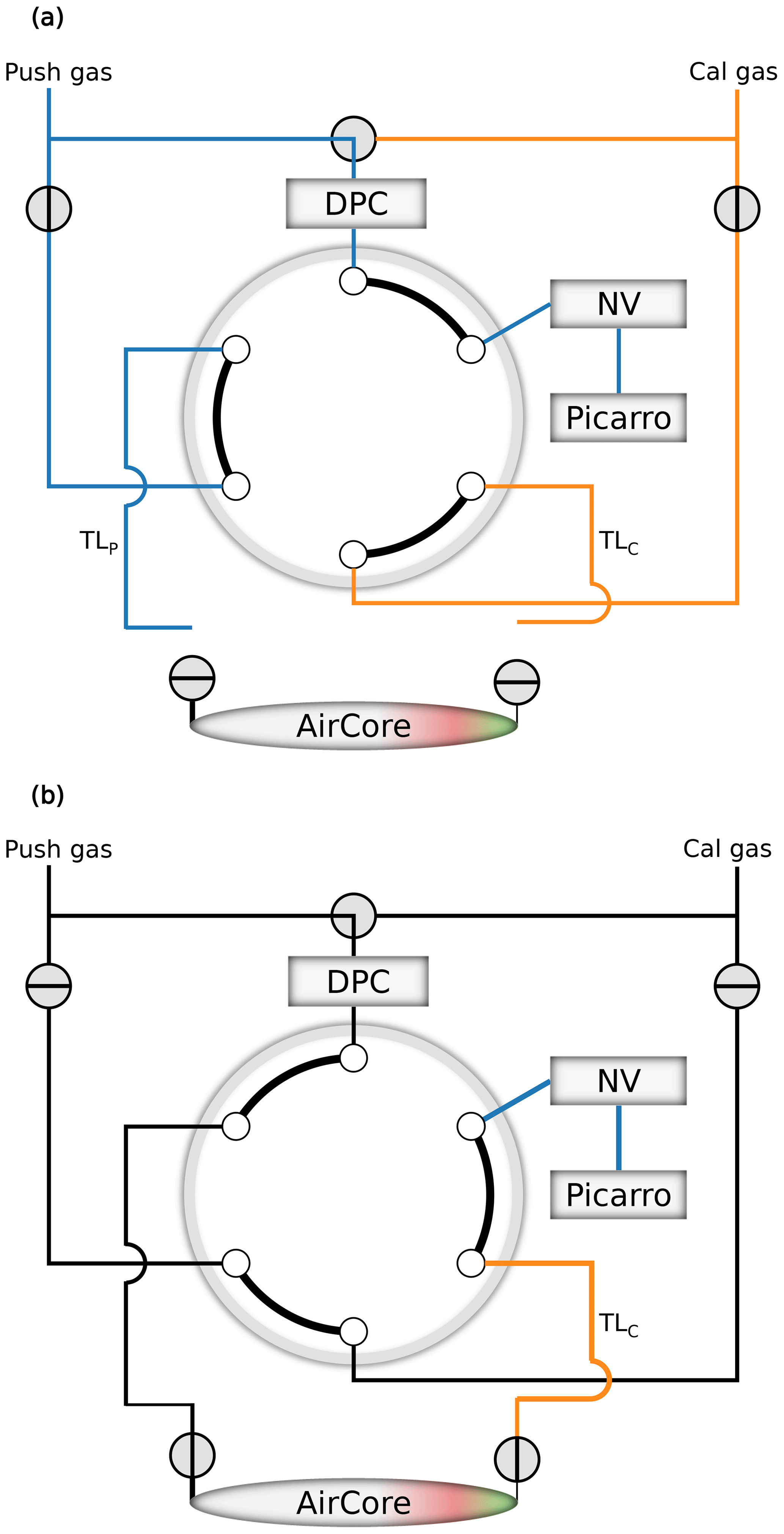
Figure 1 Analytical setup for AirCore measurements. Pressure is controlled by the digital pressure controller (DPC). Compared to the previously published setup by Engel et al. (2017), the mass flow controller has been replaced by a needle valve (NV). The Picarro operates in inlet control mode. In the bypass or flushing position (a) push gas (PG) is measured bypassing the AirCore while the transfer lines (TsL) are being flushed: TL_P with PG and TL_C with a calibration standard (Cal gas). Tubing that contains PG is indicated in blue, and Cal gas in orange. In the AirCore measurement position (b) the PG is passed through the AirCore and pushes the air to the Picarro. Directly after switching to (b), a small amount of Cal gas is measured that has been enclosed by the transfer line TL_C. For clearness, in (b) only tubing containing gas that is measured at the beginning of the AirCore analysis is colored (adapted from Engel et al., 2017).

When deployed to a weather balloon, a retrieval procedure is required, which attributes the measured trace gas mixing ratios to the sampling altitudes in order to retrieve a vertical profile. Our retrieval procedure is a three-stage process, which is reordered and refined compared to the four-stage process described in Engel et al. (2017). The overall concept of the retrieval remains the same. (i) The sampling of air during the balloon descent is calculated based on the ideal gas law. (ii) The start and end times of the AirCore measurement in the analyzer time series are determined. (iii) The sampling and the analysis can be matched based on the molar amount. Steps (i) and (iii) are still performed according to Engel et al. (2017) and are shortly described in the following. (i) Under the assumption of an instantaneous pressure equilibrium the molar amount n of an ideal gas within a constant AirCore volume V at the sampling time t can be described by the ideal gas law:

$$\begin{array}{}\text{(1)}& n\left(t\right)={\displaystyle \frac{p\left(t\right)\cdot V}{R\cdot T\left(t\right)}},\end{array}$$

where p and T are the atmospheric pressure and the mean AirCore temperature, respectively, at t, and R is the general gas constant. The relative amount of gas n_rel is then described by

$$\begin{array}{}\text{(2)}& n_{\mathrm{rel}}\left(t\right)={\displaystyle \frac{n\left(t\right)}{n\left(t_{\mathrm{close}}\right)}}={\displaystyle \frac{p\left(t\right)\cdot T\left(t_{\mathrm{close}}\right)}{p\left(t_{\mathrm{close}}\right)\cdot T\left(t\right)}},\end{array}$$

with the total molar amount of gas n(t_close) at the closing time t_close of the AirCore. The data evaluation software takes into account special cases, where air can be lost during sampling. (iii) Since the analyzer is operated at a constant mass flow, the relative amount of measured gas m_rel(t^′) at the elapsed measurement time t^′ can be described as

$$\begin{array}{}\text{(3)}& m_{\mathrm{rel}}\left(t^{\prime }\right)={\displaystyle \frac{t^{\prime }}{t_{\mathrm{end}}^{\prime }}},\end{array}$$

with the total AirCore measurement time $t_{\mathrm{end}}^{\prime }$. By interpolating the meteorological and positional data collected during sampling from n_rel(t) to m_rel(t^′), it is attributed to the trace gas measurements χ(t^′).

In order to accurately derive m_rel(t^′), the start and end points of the AirCore analysis in the continuous Picarro measurement time series need to be known (step ii). In Sect. 2.2 we present a new approach to determine the start point of the AirCore in the measured trace gas time series. This new approach has the advantage of providing an objective start point without the need for subjective judging.

2.2 Start point determination

Membrive et al. (2017) stated that for their slowly descending high-resolution AirCore the dominating uncertainty source in the stratosphere is related to selecting the start point of the AirCore analysis in the continuous Picarro measurement time series. They link this to the low amount of stratospheric sample compared to the tropospheric sample. For AirCore samplers with less stratospheric sample, the effect can be considered to be larger. Until now, the choice of the start point relied on subjective judging (Engel et al., 2017; Membrive et al., 2017). In order to systematically evaluate the altitude attribution procedure with the CO-spiking experiment presented in this paper, as many as possible subjective parameters need to be eliminated. We therefore decided to refine the process of selecting the start time of the AirCore and introduce a new approach to identify an accurate start point without the need for subjective judging.

For a regular GUF setup AirCore flight analysis, we first measure PG (high CO, 1.4 ppm in the recent GUF campaigns). We then switch the two-position valve (see Fig. 1b) like described in Engel et al. (2017) so that secondly the measurements gradually approach the low CO mixing ratio of the calibration gas (Cal gas, 0.2 ppm in the recent GUF campaigns) that was left in the transfer line, TL_C, between AirCore and analyzer. Since in our setup one standard gas is used as both PG and FG, the Cal gas serves to distinguish between PG and FG in the measurement time series. Thirdly, it is followed by the remaining FG in the AirCore (high CO), which is fourthly followed by the stratospheric sample (STRAT, low CO). The resulting idealized CO mixing ratio time series including gradual transitions between gas fractions is shown in Fig. 2a. In the past, a Gaussian distribution was fitted to the FG peak in the CO measurements (Engel et al., 2017). The half maxima of the fit were then considered the start of the AirCore and the start of the STRAT, as described in Engel et al. (2017) Sect. 2.4.1 and 2.4.3. This FG peak, however, is partly mixed with PG, Cal gas and STRAT. In the new approach, we reconstruct the gas fraction time series for each of these gases, in order to separate the amount of PG, Cal gas, FG and STRAT based on the measured CO signal. This is possible due to the fact, that a sequence of gases with known CO mole fractions is measured with a constant molar flow in the considered time interval. The fraction of each gas changes during time. Figure 2b shows the idealized gas fraction time series for these four gases. We describe the fraction f_i of each gas i by a combination of two terms: one being an increasing term (f_i,up) and the other being a decreasing term (f_i,down; see Fig. 2c for an example corresponding to FG). This is also expressed in Eq. (4):

$$\begin{array}{}\text{(4)}& f_i\left(t\right)=f_{i,\mathrm{up}}\left(t\right)+f_{i,\mathrm{down}}\left(t\right).\end{array}$$

f_i,up ranges from 0 to 1, whereas f_i,down ranges from 0 to −1. For mass constancy, the decreasing term of one gas equals the increasing term of the subsequent gas multiplied by −1:

$$\begin{array}{}\text{(5)}& f_{i,\mathrm{down}}\left(t\right)=-f_{i+\mathrm{1},\mathrm{up}}\left(t\right).\end{array}$$

The increasing term of the first gas equals 1; i.e., the PG measurements at the beginning of the AirCore measurement are considered to be stable. Likewise, the decreasing term of the last gas equals 0. This way, the sum of the gas fractions of all the gases always equals 1:

$$\begin{array}{}\text{(6)}& f_{\mathrm{\Sigma }}\left(t\right)={\sum }_{i=\mathrm{1}}^n{f}_i\left(t\right)=\mathrm{1},\end{array}$$

where n is the number of considered gases. For a regular GUF setup AirCore flight, n equals 4 (i.e., PG, Cal gas, FG and STRAT). The gas fraction time series of all of the gases multiplied by their respective CO mixing ratio χ_i,CO yields the actual measured CO mixing ratio time series of the Picarro χ_CO(t):

$$\begin{array}{}\text{(7)}& {\mathit{\chi }}_{\mathrm{CO}}\left(t\right)={\sum }_{i=\mathrm{1}}^n{f}_i\left(t\right)\cdot {\mathit{\chi }}_{i,\mathrm{CO}}.\end{array}$$

χ_i,CO of STRAT is approximated for each flight by taking the mean of a measurement section of the AirCore that is subjectively considered to be as unaffected as possible from mixing with FG and tropospheric air.

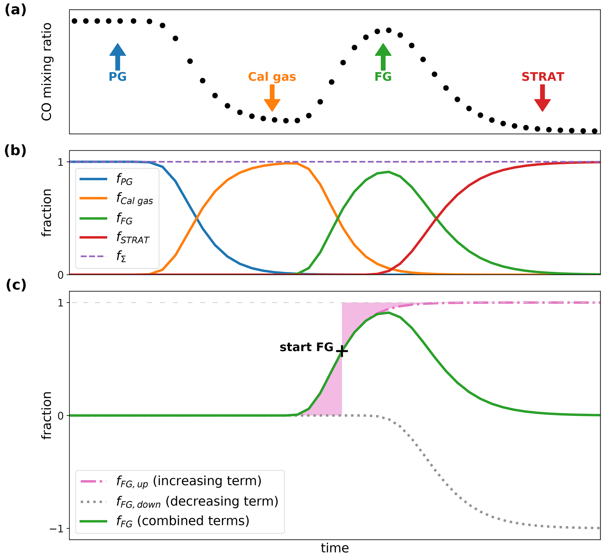
Figure 2 Idealized time series at the start of a GUF AirCore measurement with a Picarro CRDS. (a) CO mixing ratio time series. (b) Gas fraction time series of push gas (PG), calibration gas (Cal gas), fill gas (FG) and stratospheric sample (STRAT) corresponding to (a). f_Σ is the sum of all fractions and always 1. (c) Example time series of increasing and decreasing term for the FG fraction. At the starting point “start FG”, the two areas of the increasing term indicated in pink are of equal size.

Gkinis et al. (2010) and Stowasser et al. (2014) used the cumulative distribution function (CDF) of a lognormal distribution to fit a stepwise change in mixing ratios that is smoothed only by mixing in the analyzer cell of a Picarro CRDS. In our case we found that the transition from one gas fraction to the next can be well described by a CDF of a Gumbel distribution:

$$\begin{array}{}\text{(8)}& -f_{i,\mathrm{down}}\left(t\right)=f_{i+\mathrm{1},\mathrm{up}}\left(t\right)\approx e^{-e^{-\left(t-{\mathit{\mu }}_i\right)/{\mathit{\beta }}_i}},\end{array}$$

where μ is the mode of the respective Gumbel distribution (i.e., the inflection point of the CDF) and β is a measure for the standard deviation. Strictly speaking, the CDF of a Gumbel distribution does not start from exactly 0 – which in reality should be the case for the FG fraction due to being closed off. Albeit, we found that it reliably generates satisfying results. For simplicity of the fitting process, we decided to use the CDF of the Gumbel distribution instead of the CDF of the lognormal distribution. By altering the parameters μ_i and β_i simultaneously for each gas taking into account Eq. (8), a CO mixing ratio time series is calculated following Eq. (4) and then Eq. (7) and fitted to the CO mixing ratio time series actually measured by the Picarro analyzer. The start of the remaining FG t_FG in the measurements is the point in time, when the integral over the respective increasing term equals the integral over the remaining associated decreasing term:

$$\begin{array}{}\text{(9)}& \underset{-\mathrm{\infty }}{\overset{t_{\mathrm{FG}}}{\int }}{f}_{\mathrm{FG},\mathrm{up}}\left(t\right)\mathrm{d}t=\underset{t_{\mathrm{FG}}}{\overset{\mathrm{\infty }}{\int }}\left(f_{\mathrm{Cal}\mathrm{gas},\mathrm{down}}\left(t\right)+\mathrm{1}\right)\mathrm{d}t.\end{array}$$

In other words, t_FG is the point in time, when the amount of already passed FG (and possibly stratospheric sample) through the measurement cell equals the amount of remaining Cal gas (and possibly PG) in the cell (see also Fig. 2c, “start FG”).

Accordingly, the start of stratospheric sample t_AC is the point in time, when

$$\begin{array}{}\text{(10)}& \underset{-\mathrm{\infty }}{\overset{t_{\mathrm{AC}}}{\int }}{f}_{\mathrm{STRAT},\mathrm{up}}\left(t\right)\mathrm{d}t=\underset{t_{\mathrm{AC}}}{\overset{\mathrm{\infty }}{\int }}\left(f_{\mathrm{FG},\mathrm{down}}\left(t\right)+\mathrm{1}\right)\mathrm{d}t.\end{array}$$

The end time of the AirCore measurement in the analyzer time series t_stop is determined manually from half the transition between tropospheric sample and PG in the CO analysis data. The gas fraction time series of the FG f_fillgas(t) can be integrated over time in order to apply a sampling correction to the altitude retrieval procedure similar to Engel et al. (2017), Sect. 2.4.1. Albeit, we found this correction to only have a small impact on the resulting profiles and decided to exclude it from our retrievals. Instead, we use t_FG as the start point of the whole AirCore.

2.3 CO-spiking system setup

The CO-spiking system is an experimental setup, which can be temporarily added to any AirCore for a flight in order to evaluate the final altitude attribution. Small amounts of signal gas are pulsed in the inlet of the AirCore during descent at predefined GPS altitudes. When assigning the trace gas measurements to the sampling altitude, the CO-spike signals are assigned to a modeled altitude as well. The quality of the altitude retrieval can be evaluated by comparing the retrieved CO-spike altitudes to the release altitudes.

The CO-spiking setup consists of a signal gas reservoir, a microvalve and a connector which directly connects the microvalve to the open end of the AirCore in front of the sample drier. The adaptor is designed to have a negligible flow resistance for sampled air, while inducing only a minimal dead volume to the sampling system. We used the microvalve SMLD 300G by Gyger, which is lightweight and suited to dose signal gas volumes of around $\mathrm{1}/\mathrm{4}$ cm³ at STP on the timescale of 20–100 ms, thereby influencing the sampling process during descent as little as possible. Figure 3 illustrates the mounting hardware for the microvalve.

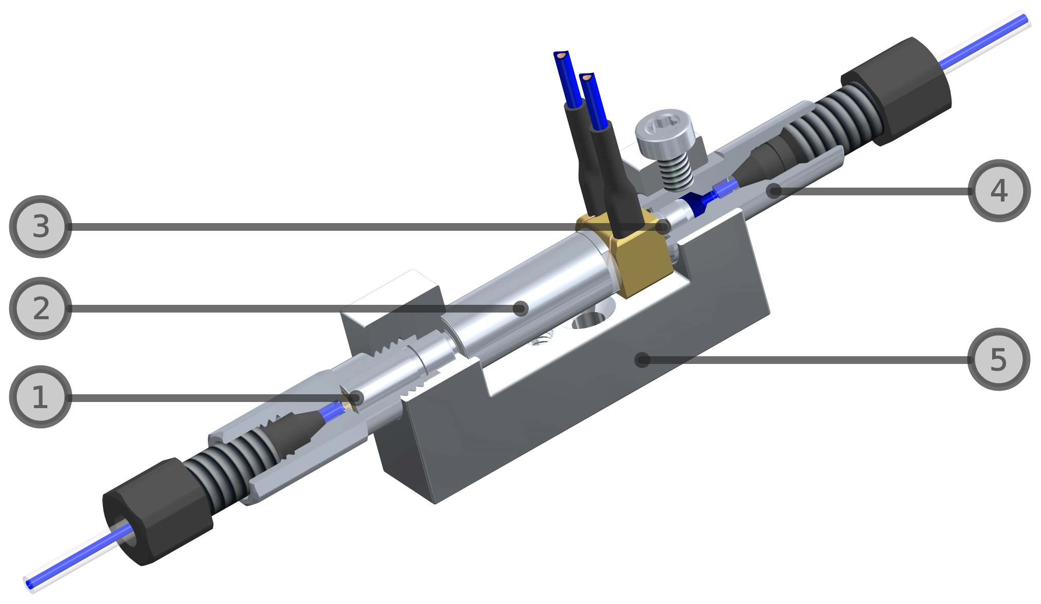
Figure 3 Mounting hardware for the SMLD 300G microvalve. (1) microvalve, (2) valve coil, (3) O-ring (material: Viton), (4) inlet adapter, and (5) valve holder. Fritz Gyger AG 2020.

We utilized a modified nylon compression ring and an additional O-ring (Fig. 3, (3)) to achieve a leak-tight seal at low temperature. In addition, the microvalve is heated during flight in order to maintain a leak-tight seal and maintain its functionality. The signal gas reservoir consists of a 2 m tubing (total volume approximately 50 cm³) and a particle filter. The particle filter protects the microvalve from particles that might have entered the signal gas reservoir. The signal gas reservoir is coiled and packed together with the AirCore in the Styrofoam box and directly connected to the microvalve. It can be pressurized via a valve at the other end of the tube and flushed by activating the microvalve. For flight preparation, the signal gas reservoir is pressurized from a signal gas canister with approximately 0.4 MPa, which is flushed by activating the microvalve and then pressurized again. The signal gas has a very high mixing ratio of CO (in our case approx. 90 ppm) compared to typical atmospheric mixing ratios so that measurable and discernible spikes can be generated with very small volumes of signal gas. During flight the microvalve is controlled by the custom made AirCore onboard electronic system to release signal gas spikes at predefined GPS altitudes. After the retrieval, the AirCore sample is analyzed for trace gas mole fractions and attributed to the meteorological and altitude data like a regular AirCore sample, for example, by following Sect. 2.1. When determining the starting point of the sample during analysis of the AirCore CO-spiking flight data following Sect. 2.2, the first CO spike is included in the gas fraction reconstruction process, as it can still overlap with the descending FG. Hence n in Eq. (6) equals 6 (i.e., PG, Cal gas, FG, STRAT, signal gas, STRAT2).

3 Results

3.1 Measurement flights

We conducted two CO-spiking flights with our AirCore GUF003 during the AirCore campaign in Traînou in June 2019. This was one of two intensive AirCore campaigns in the context of the EU-funded project RINGO (Readiness of ICOS for Necessities of integrated Global Observations), where ICOS represents the Integrated Carbon Observation System.

Table 1 Release altitudes (km) and microvalve open times (ms) for the different spikes for the two flights on 17 June and 18 June 2019 in Traînou.

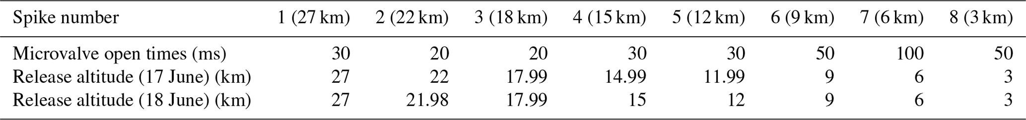
The AirCore (GUF003) was prepared following Engel et al. (2017). In addition, the CO-spiking system was set up following Sect. 2.2. The FG which we also used as PG, contains high CO (approximately 1.4 ppm) relative to clean atmospheric air in order to be well distinguishable from both tropospheric and stratospheric air. The Cal gas contains approximately 0.15 ppm CO and is used to distinguish between PG and FG at the beginning of the AirCore analysis. The gas mixture that was utilized as signal gas contains approximately 90 ppm of CO, which is almost 2 orders of magnitude higher than the CO in the FG. The microcontroller was programmed to open the microvalve at predefined GPS altitudes for a certain amount of milliseconds. Table 1 lists the release altitudes and microvalve open times for each CO spike.

The first flight was on 17 June, with launching time of 08:25 UTC. The payload was 3.5 kg and comprised the AirCore GUF003, a M10 radiosonde and a large parachute. The balloon burst at 09:50 UTC at 33.3 km and the payload landed 51 min later. The AirCore was brought back to the laboratory and started to be analyzed 2 h after landing. The second flight was on 18 June, with launching time of 07:59 UTC. The payload was similar to the first flight, but instead of a large parachute, two smaller ones were used. The balloon burst at 09:27 UTC at 33.2 km and the payload landed 41 min later. The analysis started 2 h after landing. The vertical pressure profiles were calculated from in situ GPS and temperature measurements, following Dirksen et al. (2014). The descent phase of the second flight was 10 min shorter than the one of the first flight, although both reached a similar altitude and the weather conditions were similar. The flight on 18 June thus had a higher descent rate than the flight on 17 June. The descent velocity was calculated from the smoothed GPS altitude profile. Figure 4 shows the descent velocity for the two flights versus altitude.

Figure 4 Descent velocities for the CO-spiking flights calculated from the GPS altitude time series on 17 June (dark, dashed line) and 18 June (light, dashed-dotted line), Traînou, 2019. The data are smoothed with a Savitzky–Golay filter.

Both descent velocity profiles have a similar shape. At the top of the profile (when the balloon just burst) the payload accelerates within a few hundred meters to reach its maximum speed of approximately 50 m s⁻¹ (70 m s⁻¹) on 17 June (18 June). While descending, the payload decelerates due to the increasing air resistance, reaching 4–6 m s⁻¹ in the lower troposphere. The descent velocity of the second flight was continuously higher than that of the first flight, most likely caused by the differences between the used parachutes. Since the AirCore needs a certain amount of time to equilibrate with ambient air, a high descent velocity is expected to impact the altitude retrieval based on a pressure equilibrium assumption to a larger extend than a low descent velocity. Hence, we expect the resulting calculated vertical profile of the second flight to be stretched more to higher altitudes than the one of the first flight.

3.2 Altitude attribution vs signal gas release altitude

The Picarro analyzer's mixing ratio time series was attributed to the meteorological flight data according to Sect. 2.1. Figure 5 shows the resulting vertical profile of CO mixing ratios with signal gas spikes on (a) 17 June and (b) 18 June. All eight spikes that were released at different altitudes (see Table 1) are distinguishable from the baseline data in both flights. Above approximately 20 km the baseline CO is enhanced due to mixing with FG (Engel et al., 2017) and signal gas. Below approximately 12 km the baseline CO is constantly higher than between 12 and 22 km, indicating higher CO mixing ratios in the troposphere than in the stratosphere. The signal gas spikes are fitted with a Gaussian distribution and the position of the maximum is identified to be the retrieved signal altitude. Table 2 lists the differences between the GPS release altitudes from the data logger and the retrieved signal altitudes Δh.

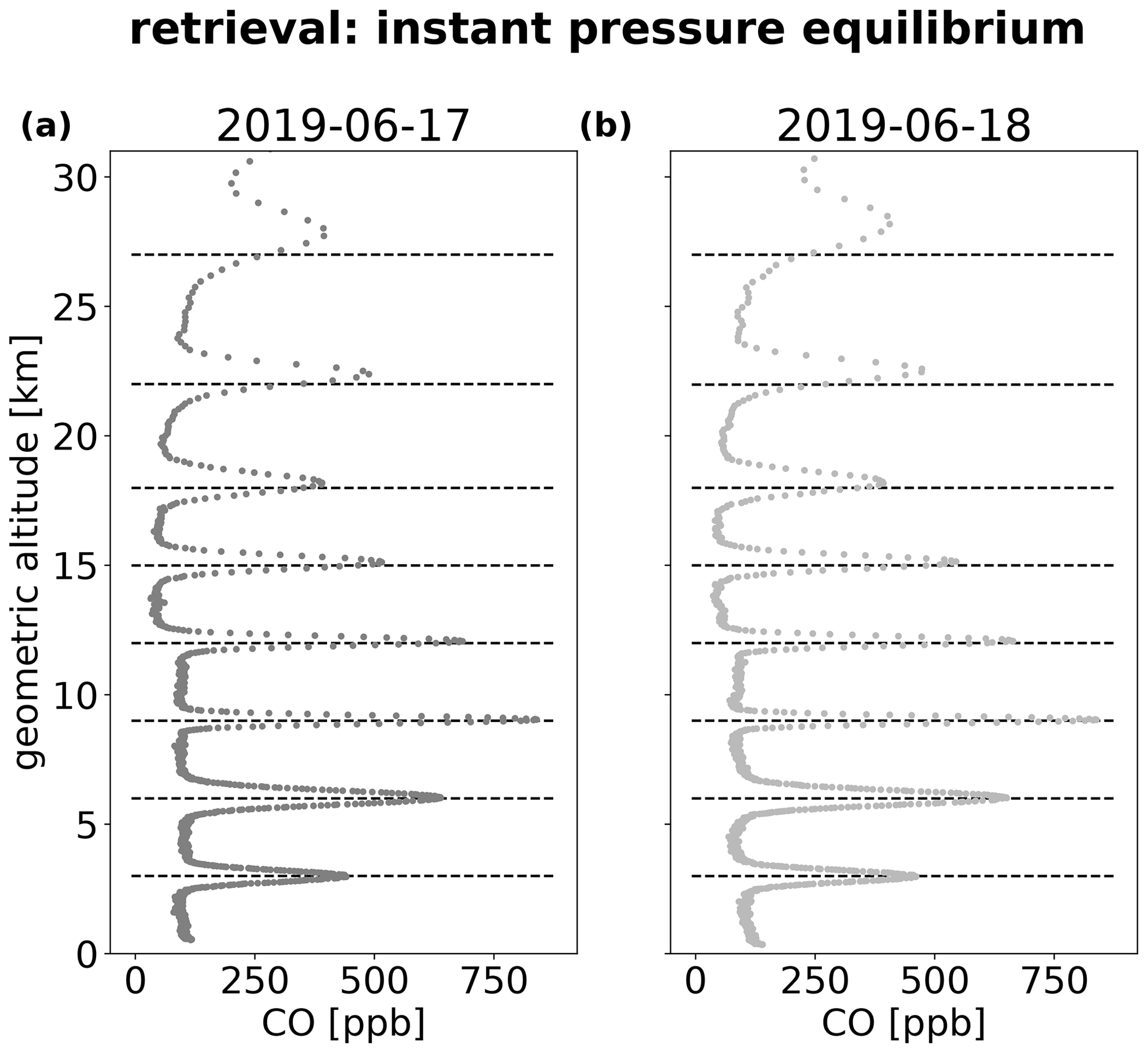
Figure 5 CO vertical profiles with signal gas spikes. (a) 17 June and (b) 18 June, Traînou, 2019. The dashed lines indicate the signal release GPS altitudes. CO measurements are attributed to geometric retrieval altitudes assuming an instantaneous pressure equilibrium between AirCore and ambient air during sampling.

Table 2 Differences between GPS release altitudes and retrieved signal altitudes Δh.

For the altitude retrieval, we assume an instantaneous pressure equilibrium. Making this assumption, the sampling altitude is overestimated more at high altitudes than at low altitudes. The overestimation is more pronounced for the flight on 18 June which had higher descent velocities. There are three major effects that lead to this. (i) The small inner diameter of AirCore samplers, the closing valve and the sample drier in general constitute a flow restriction to the inflowing air. The difference between AirCore pressure and ambient pressure is thus expected to be higher for higher descent velocities. (ii) The descent velocity is especially high at high altitudes for AirCore samplers with a parachute deployed to a weather balloon, as the low ambient pressure leads to a smaller drag by the parachute. (iii) The absolute change in ambient pressure per kilometer is lower at higher altitudes. Hence, even a small difference between AirCore pressure and ambient pressure can lead to a large overestimation at high altitudes.

As described in Sect. 3.1, the descent velocity during flight 2 on 18 June was generally higher than during flight 1 on 17 June. In agreement with the considerations above, Δh is larger for spikes above 20 km on 18 June than on 17 June. Below 20 km, Δh is comparable for both flights with less than 250 m. Between 20 and 27 km Δh is up to approximately 1200 m. Since there were no other relevant differences in the flight parameters, differences in Δh between both flights can be attributed to the differences in descent velocities. We want to emphasize that the results of these two CO-spiking flights are explicitly tied to the geometry of the GUF AirCore samplers with a fast descent on a parachute, assuming an instantaneous pressure equilibrium and cannot be transferred to other AirCore geometries.

3.3 Empirical altitude correction of AirCore profiles

One great potential of the AirCore technology is that it can be deployed to small, cheap and easy to launch weather balloons. This allows for measurements on a regular basis. Albeit, this involves dealing with high descent velocities especially in the stratosphere with implications for the vertical profile retrieval as shown in Sect. 3.2. It is desirable to have a method for correcting vertical profiles derived from AirCore measurements. The CO-spiking experiment can directly be used to correct the associated vertical profile. However, it is based on injecting small amounts of signal gas at the inlet of the AirCore during sampling, contaminating multiple parts of the atmospheric sample. We tested several parameters, obtained via the CO-spiking experiment, in order to find a way to correct clean vertical profiles derived from AirCore flights without the CO-spiking setup.

As shown in Sect. 3.2, the absolute difference in altitude between signal altitude and release altitude Δh varies between flight 1 and flight 2. Hence, a simple altitude offset correction would neglect the large impact of the descent velocity on Δh, when assuming an instantaneous pressure equilibrium. The actual pressure inside of the AirCore lags behind the changing ambient pressure during descent. This time lag Δt is observable via the CO-spiking experiment for each spike. It is the flight time of the AirCore between the theoretically retrieved altitude and the signal release altitude. Figure 6 shows Δt as a function of geometric altitude for both flights. Remarkably, Δt does not vary much between the two CO-spiking measurement flights. We applied a linear fit to the Δt–altitude relation for each flight. The resulting slope is 0.96 ± 0.05 s km⁻¹ (0.91 ± 0.06 s km⁻¹) for the flight on 17 June (18 June). Since both slopes are within one standard deviation of the respective other one, we concluded that differences between both Δt–altitude relations are insignificant and therefore applied a linear fit to the combined Δt–altitude dataset, resulting in a slope of 0.94 s km⁻¹. The maximum difference between the fit and the data is 2.5 s, which is close to the interval between two flight data records of 1 s and corresponds to an uncertainty of 150 m for a descent velocity of 60 m s⁻¹ and of 25 m for a descent velocity of 10 m s⁻¹. We used the fitting parameters (slope and intercept) to correct each of the two vertical profiles, by gradually shifting the sampling time series from Sect. 2.1 step (i). Firstly, for each record i of the sampling time series, Δt_i was calculated as a linear function of the corresponding altitude, using the fit parameters mentioned above. Secondly, the amount of sample for each record i was updated with the amount of sample that was calculated via the ideal gas law for the record Δt_i earlier in the time series. Figure 7 shows the resulting corrected vertical profiles of the CO measurements, with the same fit parameters applied to both profiles. All eight CO spikes in both profiles match the release altitudes within less than 100 m. We also tested applying the fit parameters obtained from only fitting the respective other flight's observed Δt–altitude relation. Again, all eight CO spikes in both profiles match the release altitudes within 120 m.

Figure 6 Time lag Δt between retrieved geometric altitude and signal release GPS altitude.

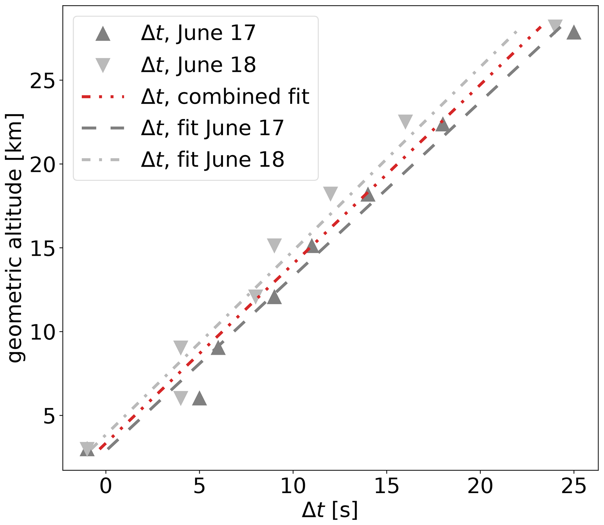
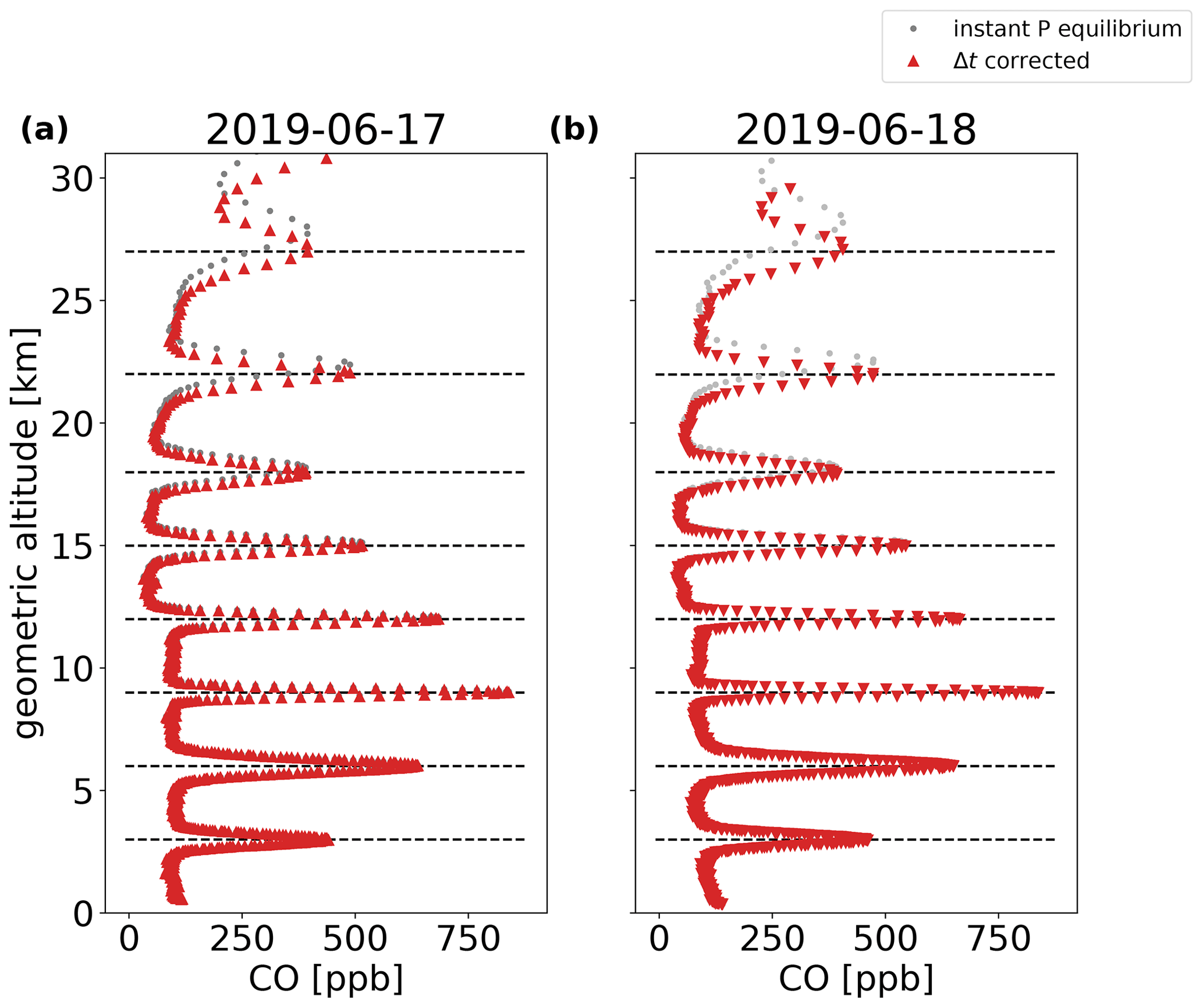
Figure 7 Corrected CO vertical profiles with signal gas spikes on (a) 17 June (red triangles pointing upwards) and (b) 18 June (red triangles pointing downwards), Traînou, 2019. The dashed lines indicate the signal release GPS altitudes. CO measurements are attributed to geometric retrieval altitudes assuming an instantaneous pressure equilibrium between AirCore and ambient air during sampling (data from Fig. 5 shown as grey circles). The individual profiles were corrected with Δt from the combined data.

Despite comprising only two measurement flights, our findings strongly suggest that Δt is a robust empirical parameter which is characteristic for a specific AirCore and applicable to flights with different descent velocity profiles. The CO-spiking experiment thus may be used to characterize a specific AirCore geometry, in order to apply an empirical correction to altitude retrievals based on assuming an instantaneous pressure equilibrium. Once an AirCore is characterized via the CO-spiking experiment, all vertical profiles from different flights of this AirCore could be empirically corrected, without contaminating the atmospheric air sample with signal gas. Albeit, further measurement flights need to be conducted in order to verify if this hypothesis holds true for flights with other maximum altitudes and other ambient conditions (e.g., temperature profiles) and other AirCore geometries. In particular, this relationship could also change for the same AirCore when a different drier is used with significantly different flow restriction. We do not recommend using contaminated sections of the AirCore profile for atmospheric interpretation. Nevertheless, the CO-spiking system could also permanently be included in a once fully characterized AirCore setup and used to insert only one spike at the top of the profile, in order to obtain highly accurate trace gas profiles (including other trace gases than CO measured with the Picarro analyzer) with minimal signal gas contamination.

3.4 Modeled vertical resolution vs. signal width

The vertical resolution of a trace gas profile retrieved from an AirCore measurement mainly depends on mixing in the analyzer cell, Taylor dispersion and molecular diffusion inside of the AirCore (Engel et al., 2017; Karion et al., 2010; Membrive et al., 2017). The theoretical altitude resolution has been modeled for CO₂ for the GUF AirCore (Engel et al., 2017; Membrive et al., 2017). Membrive et al. (2017) used a Gaussian kernel with the theoretical altitude resolution of the GUF AirCore for CO₂ and CH₄ to degrade their measured high-resolution AirCore profile and compare it to the actual measured lower-resolution GUF AirCore profile. They found a very good agreement between the two CH₄ profiles, validating the theory behind AirCore samplers. Albeit, their final results only include profile data down to 200 hPa, corresponding to altitudes well below 13 km.

The CO-spiking system can be used to experimentally quantify the vertical resolution of the CO profile of an AirCore measurement flight and to directly compare it to the theoretical altitude resolution. The volume of signal gas is on the order of $\mathrm{1}/\mathrm{4}$ cm³ at STP per spike and thus considered very small compared to the total sample volume of 1400 cm³ at STP, with the stratospheric sample volume of 100 cm³ at STP above 18 km, with respect to the GUF AirCore. The time that the spiking valve is opened is also very short (20–100 ms) so that the original spiking signal can be considered to be of negligible width. Diffusion, Taylor dispersion and mixing in the analyzer cell broaden the signal to a Gaussian-like signal gas spike. The Gaussian signal gas spike standard deviation serves as a measure for the altitude resolution for the measurement flights. We used the same approach as Membrive et al. (2017) and Engel et al. (2017) to calculate the theoretical vertical resolution of the CO profile, taking into account a 2 h time lag between landing and analysis, the molecular diffusivity of CO in air at STP of 0.18 (Massman, 1998), an effective analyzer cell volume of 6 cm³ at STP and the in situ ambient pressure and AirCore coil temperature profiles.

Taking into account the three different inner diameters and lengths of GUF AirCore tubing, the modeled vertical resolution exhibits two steps corresponding to the junctions between two adjacent parts of tubing. Figure 8 shows the modeled vertical resolution profile as a function of altitude, the Gaussian standard deviation of the respective peak and the Gaussian standard deviation derived from the Δt-corrected profile from 17 June. Regarding the second flight on 18 June, only data from the uncorrected profile are shown, since the model data and the Δt-corrected data vary only within 30 m between the two flights. As the Δt correction leads to a compression of the vertical profile, the vertical resolution of the corrected profiles is better than that of the uncorrected profiles. In general, the vertical resolution is coarser for higher altitudes, since the amount of sample is lower for higher altitudes. At the top of the profile, the dominating effect is mixing in the analyzer cell (Engel et al., 2017). Below 19 km (resp. 8 km), the effect of molecular diffusion on the vertical resolution is larger, since the sample is stored in wider tubing. The modeled vertical resolution is generally less coarse than the vertical resolution derived from the Δt-corrected profiles, however agrees well within less than 220 m throughout the profile. This small discrepancy is probably caused by the simplified assumptions guiding the model calculations, that neglect diffusion and Taylor dispersion during the AirCore sampling process. In addition, the effect of mixing in the analyzer cell may be underestimated in the model and the junctions between different diameter parts of the AirCore might induce a small amount of additional mixing. Regarding the uncorrected vertical profiles for both measurement flights, this discrepancy becomes larger at high altitudes, where the peak shape is stretched towards higher altitudes, owing to the disequilibrium between AirCore and ambient pressure. We only observe this for the two peaks above 20 km, since the Δt-correction mostly affects the upper parts of the profiles.

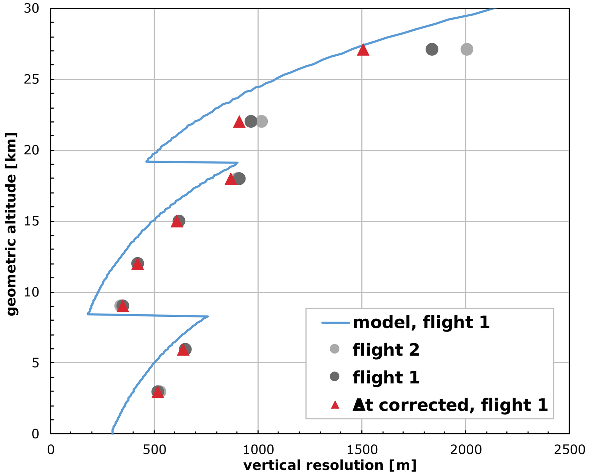
Figure 8 Modeled (blue line), uncorrected (flight 1: dark grey circles, flight 2: light grey circles) and corrected (only flight 1: red triangles) vertical resolution of GUF003.

4 Conclusions

We developed, tested and conducted an altitude-dependent CO-spiking experiment that can be used to quantitatively evaluate different combinations of AirCore geometries and retrieval procedures. It was deployed to a GUF AirCore and used to pulse small amounts of signal gas in the inlet of the AirCore during descent at predefined GPS altitudes from two weather balloon flights in Traînou in June 2019. The CO trace gas profiles were retrieved by assuming an instantaneous pressure equilibrium during the descent of the AirCore and by applying a newly introduced approach to identify an accurate starting point of the AirCore in the CO measurement time series. The comparison of the retrieved signal gas spikes with the actual signal release altitudes shows a good agreement throughout the profile with Δh being better than 250 m below 20 km. At higher altitudes the altitude of the spikes is systematically overestimated in our retrieval. This overestimation reaches up to 900 m (1200 m) at 27 km for the flight on 17 June (18 June). Both flights showed high descent velocities (up to 50 m s⁻¹ and 70 m s⁻¹, respectively), especially in the stratosphere, that differed strongly between both flights and therefore representing very different sampling conditions. The actual pressure inside of the AirCore lags behind the changing ambient pressure during descent. In the case of our AirCore, we identified this time lag, Δt, to be a possible empirical correction parameter that increases linearly with altitude and seems to be independent of the descent velocity and therefore stable among different flights. The corrected profiles showed an excellent agreement with the actual release altitudes within 120 m, even if the correction parameters derived from the respective other flight were applied. Further measurement flights need to be conducted with the CO-spiking system in order to test for the scope of validity of Δt as a robust empirical correction parameter, regarding different ambient conditions and maximum flight altitudes. Again, we emphasize that this correction will be specific for each AirCore or at least AirCore geometry. Albeit, our findings strongly suggest that an AirCore geometry- and altitude-dependent empirical Δt correction may be applied to AirCore profiles even if the payload was without the CO-spiking system once the relation has been established for a particular setup. This implies the possibility to derive trace gas profiles from AirCore measurement flights with an optimally improved altitude attribution even at high altitudes above 20 km without the need for inclusion of a spiking system during each flight. This still allows for easier operation and also provides continuous vertical profiles that have not been affected by signal gas injection.

We calculated the theoretical vertical resolution for both flights from in situ parameters including the AirCore coil temperature following Membrive et al. (2017) and compared it to the Gaussian standard deviation of the signal gas spikes. This Gaussian standard deviation serves as a measure for the in situ vertical resolution of the AirCore profile. The modeled vertical resolution is too optimistic compared to the vertical resolution derived from the Δt-corrected profiles; however, it agrees well within less than 220 m throughout the profile. This discrepancy is probably caused by the simplified assumptions guiding the model calculations. Albeit, the magnitude of the experimentally derived vertical resolution and the general shape of the resolution–altitude relation can be reproduced by the model.

Our results based on the newly developed CO-spiking system prove that trace gas profiles can be obtained from AirCore samplers deployed to low-cost weather balloons with a highly accurate altitude attribution at least up to 27 km and a fine vertical resolution, which is close to the calculations of a simple model. The quantities for Δh and the vertical resolution derived from our measurement flights are strictly bound to the GUF AirCore geometry in combination with the pressure equilibrium assumption guiding the data processing and the applied Δt correction. As an alternative to assuming an instantaneous pressure equilibrium, an altitude attribution approach has been suggested (Pieter Tans, NOAA, personal communication, 2020), which is based on modeling the pressure drop across the AirCore during sampling and the flow of air into the AirCore. When such a retrieval procedure is established, one could check if Δt is a valid correction parameter and needed for profiles retrieved in this way. The CO-spiking technique can be deployed to any AirCore and used to compare and evaluate different altitude retrieval procedures in combination with different AirCore geometries and flight platforms in future studies.