the Creative Commons Attribution 4.0 License.
the Creative Commons Attribution 4.0 License.
 | 07 Jun 2021
IMK/IAA MIPAS temperature retrieval version 8: nominal measurements
Michael Kiefer
Thomas von Clarmann
Bernd Funke
Maya García-Comas
Norbert Glatthor
Udo Grabowski
Sylvia Kellmann
Anne Kleinert
Alexandra Laeng
Andrea Linden
Manuel López-Puertas
Daniel R. Marsh
Gabriele P. Stiller
A new global set of atmospheric temperature profiles is retrieved from recalibrated radiance spectra recorded with the Michelson Interferometer for Passive Atmospheric Sounding (MIPAS). Changes with respect to previous data versions include a new radiometric calibration considering the time dependency of the detector nonlinearity and a more robust frequency calibration scheme. Temperature is retrieved using a smoothing constraint, while tangent altitude pointing information is constrained using optimal estimation. ECMWF ERA-Interim is used as a priori temperature below 43 km. Above, a priori data are based on data from the Whole Atmosphere Community Climate Model Version 4 (WACCM4). Bias-corrected fields from specified dynamics runs, sampled at the MIPAS times and locations, are used, blended with ERA-Interim between 43 and 53 km. Horizontal variability of temperature is considered by scaling an a priori 3D temperature field in the orbit plane in a way that the horizontal structure is provided by the a priori while the vertical structure comes from the measurements. Additional microwindows with better sensitivity at higher altitudes are used. The background continuum is jointly fitted with the target parameters up to 58 km altitude. The radiance offset correction is strongly regularized towards an empirically determined vertical offset profile. In order to avoid the propagation of uncertainties of O3 and H2O a priori assumptions, the abundances of these species are retrieved jointly with temperature. The retrieval is based on HITRAN 2016 spectroscopic data, with a few amendments. Temperature-adjusted climatologies of vibrational populations of CO2 states emitting in the 15 µm region are used in the radiative transfer modeling in order to account for non-local thermodynamic equilibrium. Numerical integration in the radiative transfer model is now performed at higher accuracy. The random component of the temperature uncertainty typically varies between 0.4 and 1 K, with occasional excursions up to 1.3 K above 60 km altitude. The leading sources of the random component of the temperature error are measurement noise, gain calibration uncertainty, spectral shift, and uncertain CO2 mixing ratios. The systematic error is caused by uncertainties in spectroscopic data and line shape uncertainties. It ranges from 0.2 K at 20 km altitude for northern midlatitude summer conditions to 2.3 K at 12 km for tropical conditions. The estimated total uncertainty amounts to values between 0.6 K at 20 km for midlatitude summer conditions to 2.5 K at 12–15 km for tropical conditions. The vertical resolution varies around 3 km for altitudes below 50 km. The long-term drift encountered in the previous temperature product has been largely reduced. The consistency between high spectral resolution results from 2002 to 2004 and the reduced spectral resolution results from 2005 to 2012 has been largely improved. As expected, most pronounced temperature differences between version 8 and previous data versions are found in elevated stratopause situations. The fact that the phase of temperature waves seen by MIPAS is not locked to the wave phase found in ECMWF analyses demonstrates that our retrieval provides independent information and does not merely reproduce the prior information.
- Article
(4416 KB) - Full-text XML
-
Supplement
(1668 KB) - BibTeX
- EndNote


The Michelson Interferometer for Passive Atmospheric Sounding (MIPAS) was a mid-infrared Fourier transform spectrometer operating in limb-viewing measurement geometry (Fischer et al., 2008). The spectral coverage was 4.15 to 14.6 µm (685–2410 cm−1). From June 2002 to April 2012, spectrally resolved atmospheric emission spectra were measured globally from a polar sun-synchronous orbit between 87.1∘ S and 89.3∘ N. The European Space Agency (ESA) has distributed a number of level-1b data versions that differ with respect to altitude registration, offset and gain calibration, nonlinearity correction, spectral sampling, and other issues relevant to the generation of calibrated geolocated radiance spectra. In this paper, we present vertical profiles of temperature retrieved from level-1b radiance spectra of ESA version 8.03 with the scientific level-2 MIPAS processor developed and operated by the Institute of Meteorology and Climate Research (IMK) at the Karlsruhe Institute of Technology and the Instituto de Astrofísica de Andalucía (IAA). We shall use the terms “version 8” and/or “V8” to label this data version, and the same naming conventions apply mutatis mutandis to other data versions.
From 2002 to March 2004, MIPAS recorded interferograms with a maximum optical path difference (MOPD) of ±20 cm, corresponding to a spectral resolution of 0.05 cm−1 after Norton–Beer strong apodization. This phase of operation will be called “full spectral resolution” (FR) period. Due to a technical defect, the MOPD had to be reduced to ±8 cm after March 2004, leading to a spectral resolution of 0.125 cm−1 (apodized). In turn, the vertical sampling has been increased. For this second operation phase with degraded spectral resolution, we shall use the designation “reduced spectral resolution” (RR) period.
MIPAS measurements were taken in several measurement modes. The bulk of the data were taken with the nominal measurement mode (NOM), with an altitude coverage of approximately 6–70 km, and 17 and 27 tangent altitudes for FR and RR, respectively. Smaller parts of the data comprise a mode tailored for upper troposphere and lower stratosphere measurements (UTLS-1) with 19 tangent altitudes between 6 and 50 km. Further modes are designed for middle and upper atmosphere and for noctilucent cloud measurements. Respective documentation of retrievals based on MIPAS level-1b data for these measurement modes can be found in a companion paper (García-Comas et al., 2021).
A major change with respect to earlier level-1b data versions is the use of a model for the time dependency of the detector nonlinearity. The response of the MIPAS detectors has shown to become more linear with time. However, previous calibration relied solely on a preflight detector characterization. Related investigations are summarized in Sect. 2.
The spectrally resolved radiance measurements are converted into global temperature distributions. The precision and accuracy of the resulting data depends largely on the adequateness of the setup of the retrieval. Several improvements have been made with respect to this, which are discussed in Sect. 3. The uncertainty budget is presented in Sect. 4. Example results are shown in Sect. 5, and in Sect. 6 we summarize our findings, critically discuss the success of the attempt to improve the MIPAS temperature retrieval, identify unsolved problems, and suggest topics for future work.
We intentionally describe the retrieval on a rather technical level in order to help the users to better understand the data and in order to provide a basis and documentation for scientists building future retrieval processors.
The long-wavelength detectors A1, A2, B1, and B2, which form the MIPAS bands A, AB, and B, are affected by nonlinearity, whereas the short-wavelength bands C and D have linear detectors. Preflight measurements of detector nonlinearity have been available and were used for calibration of all data versions up to version 6. MIPAS temperature time series of these data versions have shown drifts, which have been analyzed by Eckert (2012); Penckwitt et al. (2015); McLandress et al. (2015); Laeng et al. (2021). These drifts are attributed to an inadequate nonlinearity correction. Birk and Wagner (2010) found that detector nonlinearity is a function of time, i.e., that the detector response became more linear over the MIPAS lifetime. These authors have provided an age-dependent correction scheme, which has been applied since data version 7. Its adequacy has been proven by the fact that it removes the major fraction of the drifts found in previous data versions. For ozone, it has been shown that application of this new correction scheme improves the long-term stability (Laeng et al., 2018). However, temperature validation has revealed that the version 7 nonlinearity correction led to too low temperature values for the FR measurement period (Hubert et al., 2016). Therefore, the nonlinearity correction has been reviewed again, and the estimate for the modulation efficiency has been improved (Kleinert et al., 2015). This leads to generally higher radiances and a better agreement with the validation data.
A further change in the calibration procedure refers to the selection of calibration spectra. While up to version 7 the gain calibration was updated only once per week, in version 8 all available gain calibration measurements were used, which is usually one gain measurement per day. Thus, most version 8 MIPAS radiance spectra rely on calibration spectra from the same day. In the case that MIPAS operation was interrupted, care was taken that the gain measurements closest in time from the same instrument state were applied.
In this paper, the most recent temperature data versions generated with the MIPAS processor developed and operated at the Institute of Meteorology and Climate Research (IMK) in cooperation with the Instituto de Astrofísica de Andalucía (IAA) are discussed. The IMK-IAA data processor relies on multi-parameter nonlinear least-squares fitting of measured and modeled spectra (von Clarmann et al., 2003a). Its extension to retrievals involving non-local thermodynamic equilibrium emissions is described in Funke et al. (2001), while the adaption to the RR measurements is documented in von Clarmann et al. (2009b). In the following we discuss all retrieval settings relevant for temperature, which is retrieved along with the tangent altitude of the line of sight. The pressure–altitude relation is not derived from the spectra directly but rather calculated for each iteration with the hydrostatic approximation based on the current guess of temperature profile and a pair of pressure and geometrical altitude values taken from the a priori profile at 20 km or above (see Sect. 3.4). The combined temperature and tangent altitude retrieval is the first step in the chain of retrievals and is preceded only by the determination of a frequency shift (see Sect. 3.2).
3.1 Retrieval method
In order to put the improvements discussed later into the context of the pre-existing retrieval scheme, we recapitulate the main features of the MIPAS temperature retrieval scheme here. MIPAS spectra are analyzed with a constrained nonlinear least-squares fit. The updated guess of the state vector xi+1 at iteration i+1 is calculated from the previous estimate xi as follows:
Here K is the Jacobian containing the partial derivatives , superscript “T” indicates transposed matrices, Sy,noise is the covariance matrix representing measurement noise, R is a regularization matrix, y is the vector of measurements under consideration, F(xi) is the vector of the respective simulated measurements based on the Karlsruhe Optimized and Precise Radiative Transfer Algorithm (KOPRA, Stiller, 2000), and xa is the vector of prior information on x. The vertical grid for the retrieval of the temperature profile is 0, 4[1]50, 52[2]70, 72.5[2.5]80, 85[5]110, 120 km (i.e., lower altitude [altitude step] upper altitude). MIPAS measurements are analyzed limb profile by limb profile in a global-fit mode in a sense that all fitting residuals related to an entire limb scan are minimized simultaneously rather than in sequence (Carlotti, 1988). Contrary to the original global-fit approach, which was an un-regularized maximum likelihood retrieval, we do use regularization (Sect. 3.3). Adequate a priori information above the uppermost MIPAS tangent altitude proved to be of particular importance (Sect. 3.4). Also contrary to the original global-fit method, our retrieval scheme supports consideration of horizontal variability along the line-of-sight direction (Sect. 3.5), where the respective element of x associated with a certain altitude is a scaling factor for the horizontal temperature distribution. Temperature is fitted jointly with a correction of the tangent altitude of the line of sight in order to minimize mutual error propagation. During each iteration, a hydrostatic atmosphere is constructed using the current guess of the temperature profile and pointing information. For this purpose, a reference point from the a priori temperature profile is used for which geometrical altitude, pressure, and temperature are available (see Sect. 3.4 and von Clarmann et al., 2003a, for further details). The temperature and tangent altitude fit uses spectral lines of CO2 because excellent prior knowledge on the vertical distribution of this gas is available and because no rapid changes in its mixing ratios are expected. The retrieval relies on specific parts of the spectra, called “microwindows”, which contain maximum information on the target quantities with minimal contributions from gases of unknown abundance (see Sect. 3.6). This means that y contains only a subset of the available spectral measurements. However, CO2 lines are not perfectly isolated but are interfered with by a background continuum and some signal of mainly H2O and O3. To avoid propagation of uncertainties of the a priori uncertainties of these gases and the background continuum, these parameters are jointly fitted with the temperature and tangent altitude information, i.e., they are part of the x vector (Sect. 3.7 and 3.9, respectively). In addition, an additive offset calibration correction is retrieved, which is frequency-independent for each microwindow (Sect. 3.8). An accurate retrieval depends crucially on the choice of reliable spectroscopic data (Sect. 3.10). Consideration of non-local thermodynamic equilibrium emission improves the retrieval at higher altitudes (Sect. 3.11). Adequately chosen numerical accuracy parameters are important for a sound trade-off between the accuracy of the results and computational efficiency (Sect. 3.12).
Previous MIPAS temperature and tangent altitude retrievals were described in von Clarmann et al. (2003a) for FR measurements and in von Clarmann et al. (2009b) for RR nominal-mode version 4 measurements. The RR upper troposphere–lower stratosphere measurements mode version 4 retrievals were documented by Chauhan et al. (2009). RR version 5 nominal-mode retrievals were presented by von Clarmann et al. (2013). Version 3 temperatures were validated by Wang et al. (2005, 2004), while version 5 temperatures were validated by Stiller et al. (2012).
3.2 Frequency calibration
Prior to the retrieval of atmospheric state variables, a frequency shift scale is determined from the spectra. In principle, the level-1b data are already frequency-calibrated, but frequency calibration and instrument line shape modeling are intertwined. For our retrieval we need an adjustment of the frequencies that also accounts for any frequency shift implied by the modeling of the instrument line shape.
A technical change with respect to the frequency calibration has been implemented in the level-1b processing. Instead of one spectral calibration per four scans, spectral calibration in version 8 is performed once per day, relying on measurements of one full orbit. The mean spectral shift scale is then applied to all measurements of the respective day. The MIPAS spectral accuracy of ESA's frequency calibration is estimated to 0.00065 cm−1 at 2410 cm−1 (Kleinert et al., 2018). The described modification of the frequency calibration scheme leads to very small differences in the retrieved atmospheric state variables and is of minor relevance to the IMK/IAA MIPAS processing because a spectral shift correction is performed as the first step of the retrieval chain anyway.
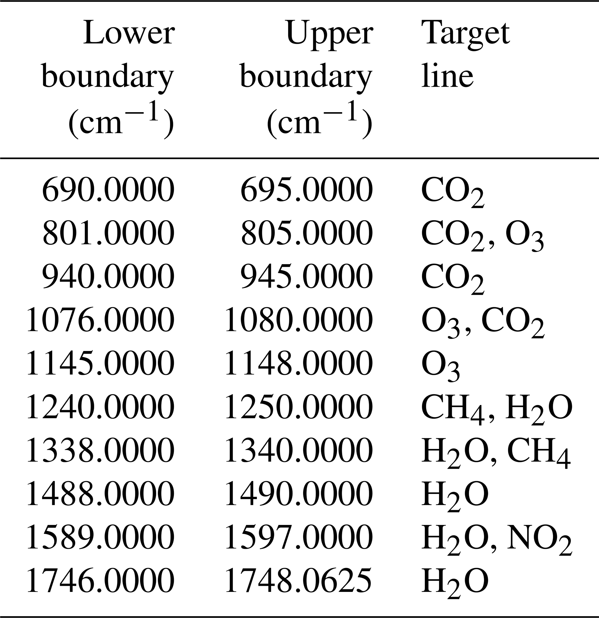
The calculation of the spectral shift within the IMK-IAA processing is made by minimizing the residual between simulated and measured spectra using Eq. (1) and then fitting a linear regression function to the shift values, which are calculated for the single microwindows. Differences between calculated shift values and the values represented by the fitted line range from cm−1 to 0.00032±0.00032 cm−1 with a root of the mean square value over all frequencies of 0.00039 cm−1. The microwindows used for the frequency shift retrieval are shown in Table 1. Line selection criteria were sufficient line strength, good separation of the target lines, and a good coverage of the MIPAS A, AB, B, and C bands. The MIPAS D band was not used because sufficiently strong D-band transition would require consideration of non-local thermodynamic equilibrium in the respective radiative transfer calculations, which was considered too costly for this purpose.
Table 1Microwindows for the retrieval of residual spectral shift.
For the frequency scale correction, we use spectra at a tangent altitude of 38 km, where the lines are narrow enough to allow for a good spectral calibration and where the signal is still strong enough to avoid large random error in the spectral shift correction. Under some polar winter conditions, and particularly in the case of an elevated stratopause, however, the shift retrieval from a single spectrum is by far not precise enough. In order to reduce large fluctuations due to noise, the spectral shift retrieval is constrained towards its temporal mean, where separate means were used for the high-resolution measurement period and the reduced-resolution measurement period. The reason for this choice was the use of different instrument line shapes for these measurements.
Inclusion of NO2 proved to be essential, particularly because of a sizable signal of mesospheric NO2. Omission of this gas would lead to artificial diurnal variations of the spectral shift.
The fit is carried out using a maximum a posteriori scheme (Rodgers, 2000) using the mean of the spectral calibration scale over the entire FR and RR period, determined in a previous step as a priori. A priori variances of (0.00035 cm−1)2 for the FR and (0.0007 cm−1)2 RR measurements are used. The actual spectral correction for any wavenumber can be determined using the linear regression function.
3.3 Regularization
According to the retrieval vector x, R has a block-diagonal structure, and the choice of the regularization can be made independently for each group of variables.
In general we use a regularization term, which is composed of a smoothing component Rsmooth and a diagonal component Rdiag:
Here the diagonal component Rdiag is formally equivalent to the inverse of an a priori covariance matrix without information on inter-altitude correlations. For the regularization term Rsmooth the following implementation of the altitude dependence has replaced the approach by Steck and von Clarmann (2001), which has been used in our retrievals up to version 5.
Here L is an first-order finite-difference operator as suggested by Tikhonov (1963), Twomey (1963), and Phillips (1962) but scaled with the respective grid width to yield difference quotients. The γ values control the altitude dependence of the strength of the regularization.
The regularization term used for the parameter temperature is RT=Rsmooth with the values of all γi being set to 0.49 K−2 in the entire altitude range.
The tangent altitudes are constrained towards the line-of-sight engineering information. The respective block of R can be understood as an inverse a priori uncertainty covariance matrix describing both the relative pointing uncertainties between adjacent tangent altitudes and the absolute pointing uncertainty of the entire limb scan as a whole. The relative pointing a priori uncertainties were assumed to be 60 m in the RR measurement mode and 150 m in the FR measurement mode, in terms of 1σ standard deviations. The standard deviation of the absolute pointing uncertainty, representing the possible altitude shift of the entire limb scan, was assumed to be 900 m.
3.4 A priori temperature and trace gas distributions
In older nominal-mode retrieval versions problems occurred which could be traced back to the use of inadequate a priori temperature distributions for altitudes above the uppermost MIPAS tangent altitude. Here, reliable analysis data are not available, and MIPAS cannot vertically resolve the temperature profile. Older retrieval versions used the NRLMSISE-00 climatology (Picone et al., 2002) at these altitudes. However, this climatology has systematic biases (Emmert et al., 2020) and does not capture short-term variations occurring in dynamically active episodes such as elevated stratopause events. Due to missing MIPAS measurement information at related altitudes, this error propagated into the MIPAS temperatures in the nominal scan range. These temperature retrieval errors further propagated noticeably into retrievals of trace species, e.g. ozone (Laeng et al., 2018).
For IMK/IAA MIPAS version 8 temperature retrievals, ECMWF ERA-Interim analysis fields (Dee et al., 2011) were used as a priori at altitudes up to 43 km because ERA-5 was not available for the MIPAS time period when the processing was started. A priori temperatures above 53 km are based on Whole Atmosphere Community Climate Model (WACCM, Marsh, 2011; Marsh et al., 2013) Version 4 (WACCM4) fields of a specified dynamics run (García et al., 2017), which provided output specifically for the MIPAS measurement geolocations and times. Since a specified dynamics run was used, the actual atmospheric conditions, including stratospheric warming events and elevated stratopauses, were sufficiently well reproduced. The WACCM temperatures were bias-corrected using MIPAS version 5 middle and upper atmosphere measurements, which cover an altitude range of 18–102 km but are performed less frequently (García-Comas et al., 2014). Multi-annual averages of MIPAS-colocated WACCM differences were used to construct an altitude- and latitude-dependent seasonal correction, independently for day and night observations. The transition between ECMWF and bias-corrected WACCM takes place between 43 and 53 km. In this altitude region the temperature is calculated as the average of the two contributing profiles with altitude-dependent weights. The pressure above 43 km is calculated by numerical integration of the hydrostatic equation starting with the ECMWF value at 43 km. The integration uses the mixed temperature profile up to 53 km and the bias-corrected WACCM temperature above, as well as the corresponding given geometric altitudes. The pressure–altitude relation at 20 km altitude (or at the lowest tangent altitude above 20 km with valid spectral information), which is assumed to be fixed for the calculation of the pressure profile by the hydrostatic equation during the retrieval iterations, is taken from this a priori profile (for details, see Sect. 2.2. of von Clarmann et al., 2003a).
CO2 distributions are imported from an SD-WACCM4-based climatology. From MIPAS V5 data, gas profiles are generated for interfering species and for initial guess profiles for O3 and H2O, which both are jointly fitted together with target state variables. The a priori of the latter is a zero profile, while the regularization is of Tikhonov type.
3.5 Horizontal variability
Typically, a locally spherically symmetric atmosphere is assumed in profile retrievals. That is to say, within one profile retrieval the atmospheric state is assumed to be a function of altitude only and does not vary with latitude or longitude. However, for MIPAS limb measurements the range where 95 % of the information originates from varies from about 260 to 440 km (von Clarmann et al., 2009a). Hence, the horizontal homogeneity assumption is not without problems. Depending on the computational effort spent on accurate radiative transfer modeling, a fully tomographic retrieval as suggested by Carlotti et al. (2001, 2006) or Steck et al. (2005) is often beyond reach. As a first step, horizontal inhomogeneities of temperature have been considered in the trace gas retrievals since MIPAS version 4 by retrieving a horizontal temperature gradient applicable in a range of ±400 km around the tangent point (Kiefer et al., 2010). For retrievals based on level-1b spectra of version 7 onwards, we go a step further and consider a full a priori 3D temperature field generated from ECMWF ERA-Interim data with latitude and longitude resolutions of approx. 1.1∘, extended by NRLMSISE-00 data above 60 km. During the retrieval, the temperatures of this 3D a priori field are scaled at each altitude in a way that the horizontal structure is provided by the a priori while the vertical structure comes from the measurements. The respective component of the retrieval vector x is the 1D vector of scaling factors. Roughly speaking, the result is a temperature profile which provides the best spectral fit under the assumption that the a priori horizontal structure of the temperature field is correct. The information on the horizontal temperature variability enters through the a priori, but the vertical structure is provided by the MIPAS temperature retrievals.
Additionally, the retrieval of a horizontal gradient directly from the spectra of a single limb sequence is performed. However, the horizontal gradients are strongly regularized towards zero below 60 km, where ECMWF ERA-Interim temperature fields are available, and above 70 km, the topmost tangent altitude of MIPAS nominal measurement mode. In between, the regularization of the temperature gradient is chosen to be weaker in order to better exploit the information on the horizontal temperature gradient provided by the measurements.
3.6 Microwindows
The retrieval does not use all of the measurement data but only parts of the spectra that are particularly sensitive to the target species, so-called “microwindows” (see von Clarmann and Echle, 1998, for the rationale behind this approach). For the combined temperature and tangent altitude retrieval CO2 lines are used because the mixing ratio distribution of CO2 is well known and only weakly structured. This reduces the number of unknowns in the retrieval.
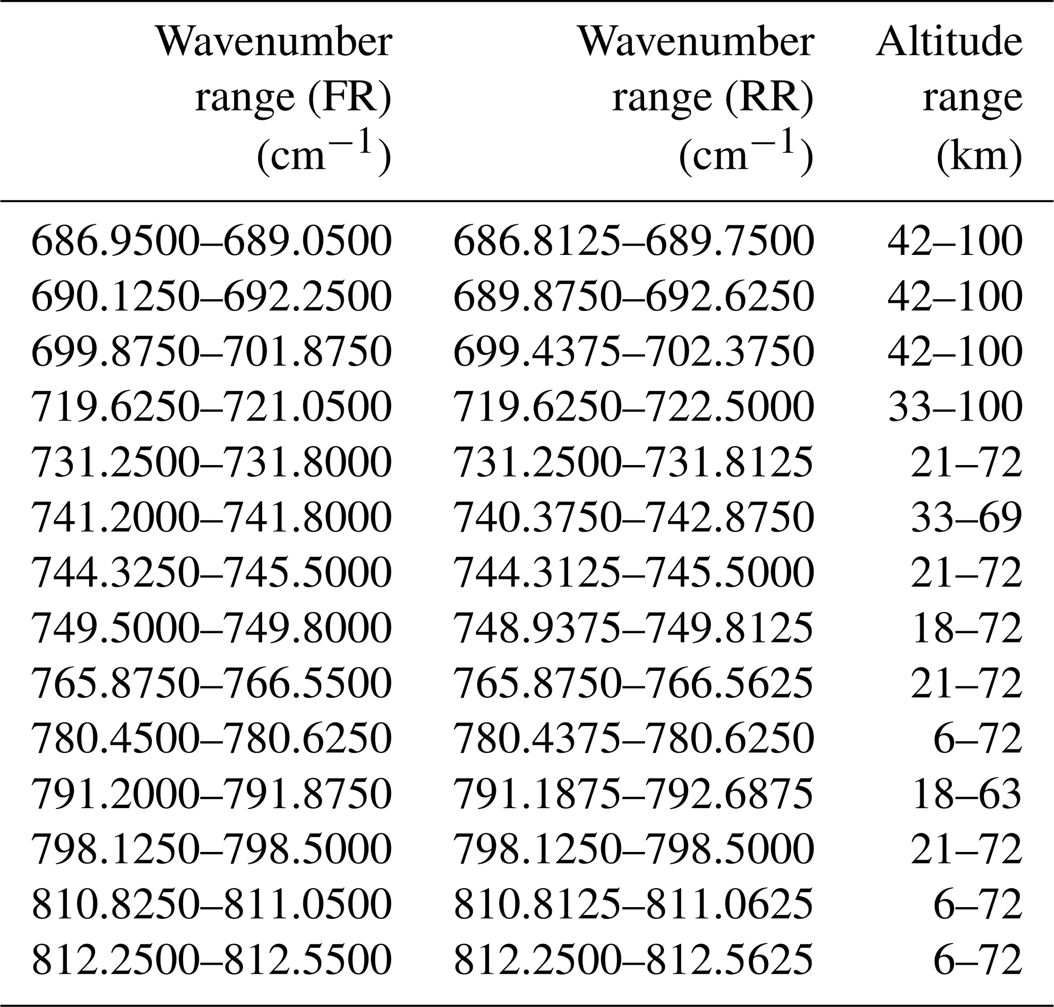
In order to have more information on temperature at high altitudes, additional microwindows were included since data version 5. These are 686.8125–689.7500, 689.8750–692.6250, 699.4375–702.3750, 719.6250–722.5000, 740.3750–742.8750, and 791.1875–792.6875 cm−1 (given for the wavenumber grid of the RR measurements). The full list of microwindows for FR and RR measurements is presented in Table 2. The inclusion of CO2 Q branches, on the one hand, implies the consideration of line mixing (omitted in previous data versions) but, on the other hand, allows the use of the same microwindow selection for analysis of MIPAS nominal and middle-atmosphere measurements (García-Comas et al., 2021). Thus, apart from the increased information gain for higher altitudes, this choice will lead to a better inter-consistency between the two datasets. Depending on the tangent altitude, certain data points within a microwindow can be discarded to avoid interference by spectral lines of gases other than CO2.
Table 2Microwindows of the combined MIPAS temperature and tangent altitude retrieval for the full (first column) and reduced (second column) spectral resolution.
3.7 The background continuum
Joint-fitting of a background radiance continuum has always been a standard feature of all MIPAS retrievals (e.g., von Clarmann et al., 2003a). The purpose of this is to account for all radiance contributions that are included neither in the line-by-line calculation of absorption cross sections nor the pressure–temperature interpolation of pre-tabulated laboratory measurements of absorption cross sections of heavy molecules. These contributions are caused by (a) the far-wing contributions of transitions spectrally distant from the analysis window under investigation, which add up to a continuum-like background signal whose line-by-line modeling would be inefficient; (b) continuum emission of trace gases by, e.g., dimers in the case of H2O; (c) differences between the idealized modeled line shapes and the true super- or sub-Lorentzian pressure broadening; and (d) the emission by non-gaseous components of the atmosphere like clouds, aerosols, volcanic ash, or meteoric dust. Since these non-line-by-line effects are mostly important in the lower atmosphere, the background continuum contribution was only fitted up to 33 km altitude in previous data versions and set to zero above. It turned out, however, that consideration of the background continuum up to altitudes of 58 km significantly improved the robustness of the retrievals and removed known biases in retrieved state variables. The cause of the continuum signal from high altitudes is possibly meteoric dust (Neely III et al., 2011). The relevance of a high-reaching continuum signal was first discovered by Haenel et al. (2015) in the context of the retrieval of SF6.
Only a smoothing constraint is applied to the continuum retrieval up to 58 km without any diagonal term. Above, the continuum is regularized exclusively by a diagonal term and an a priori of zero. Formally, an individual continuum profile is retrieved per microwindow, but the continuum values are not only constrained in the altitude domain but also in the frequency domain. The latter smoothing constraint avoids unrealistic jumps of the value of the background continuum between adjacent microwindows.
3.8 Offset correction
Besides the background continuum, we also retrieve a radiance offset profile that is meant to correct the radiance zero-level calibration. While the continuum is additive to the absorption coefficient and appears in the exponent of Beer's law, the offset correction is directly additive in the radiance space. When radiative transfer is linear, which is the case for high tangent altitudes, the offset correction and the background continuum cannot be distinguished and the simultaneous retrieval of both leads to a null-space of solutions. This problem is solved by strongly constraining the background continuum to zero above 58 km, while the vertical offset profile is strongly regularized towards an empirically determined offset correction profile (Kleinert et al., 2018), which is used as a priori for the fit of the zero-level correction. The actual offset value per microwindow and per altitude is retrieved using both Rsmooth. and Rdiag.. The diagonal term corresponds to a variance that is roughly a factor of 2 larger than the offset uncertainty obtained by Kleinert et al. (2018), in order to account for possible unknown uncertainties. No regularization of the offset in the frequency domain has been applied, i.e., the offset can vary independently between microwindows.
3.9 Joint fit of O3 and H2O
Ideally, microwindows contain only signal of the target species and are free of any interfering signal. In general, however, such microwindows do not exist. In particular, H2O and O3 have sizable contributions in the microwindows of the temperature retrieval. Since the temperature retrieval is the first step in the retrieval chain, no actual information on the highly variable trace gas abundances is available.
To avoid the mapping of inadequate assumptions on the actual H2O and O3 abundances, these species' mixing ratio profiles are jointly retrieved with temperature. Since the microwindows of the temperature retrieval have not been optimized for joint retrieval of H2O and O3, the resulting mixing ratios are discarded. The only purpose of this joint-fit approach is to avoid related error propagation.
3.10 Spectroscopy
The HITRAN 2016 spectroscopic database (Gordon et al., 2017) was used for CO2, whose lines provide the information on temperature and the tangent altitude, as well as for most interfering species. Exceptions are O3 and HNO3, for which the dedicated MIPAS spectroscopic database provided by Flaud et al. (2003) was used.
3.11 Non-local thermodynamic equilibrium
Typically, radiative transfer in the stratosphere is calculated assuming that the atmosphere is in local thermodynamic equilibrium (LTE). Test calculations, however, have provided evidence that the consideration of non-LTE (NLTE) populations of vibrational states involved in the contributing CO2 bands also makes a difference for temperature retrievals in the MIPAS nominal observational altitude range. NLTE populations of the CO2 states emitting around 15 µm, driven by absorption of upwelling radiation and insufficient collisional thermalization, occur predominantly above the nominal tangent altitude range (> 70 km); however, their emissions contribute to the radiances measured below. The non-LTE effects are only moderate here and thus a full-blown non-LTE retrieval using all the machinery developed by Funke et al. (2005) seems undue. Instead we use a non-LTE parameterization that accounts for the temperature dependence of vibrational non-LTE populations in an approximate manner (manuscript in preparation), which is briefly explained in the following.
Considering a simple two-level system under non-LTE conditions, upper- and ground-state populations n1 and n0, respectively, are related by
with the collisional productions and losses P and L, respectively, radiative losses A, and non-thermal productions R (e.g., radiative production by solar absorption). In this equation, only , with ΔE being the energy difference between upper and ground state, is temperature dependent. Hence, Eq. (4) can be separated into a temperature-dependent term and a temperature-independent term b with and .
The radiative transfer algorithm uses population ratios with . Using Eq. (4) and the identity , the population ratio r(T,z) can be expressed as function of the ratio r(T0,z) at a reference temperature T0 as
with U=a and E=ΔE for the simple case described above. An updated version of the Generic RAdiative traNsfer AnD non-LTE population algorithm (GRANADA) (Funke et al., 2012) computes the parameter profiles U(z) and E(z) for realistic and more complex situations (i.e., multi-level systems, nonlinear interactions by vibration–vibration collisions, etc.), allowing for a temperature parameterization of non-LTE population ratios in a local approximation. A seasonal and latitudinal climatology of r(T0,z), U(z) and E(z) for the local times of MIPAS ascending and descending overpasses has been calculated offline with GRANADA and is considered by the KOPRA radiative transfer model in the forward calculations (Funke and Höpfner, 2000) to estimate the non-LTE population ratios of vibrational states 01101, 02201, 10011, and 11101, involved in the observed 16C12O2 bands for the actual temperatures at each line-of-sight path segment during the retrieval iterations. This approach seems to be a fair compromise between rigor and efficiency.
3.12 Numerical issues
The accuracy of the numerical integration in the radiative transfer modeling has been improved in several places. In order to achieve a more accurate numerical integration of the radiance over the field of view, now five pencil beams are used throughout, while older retrievals (up to version 5) used only three pencil beams at some tangent altitudes. In addition, in order to improve the numerical accuracy, a finer wavenumber grid is used for calculation of the monochromatic absorption cross sections (0.00048828125 cm−1 instead of 0.001 cm−1). The convolution of the spectrum with the apodization function (Norton and Beer, 1976) now includes a wider wavenumber range. Additionally, a more conservative rejection threshold for lines so small that they are deemed not to contribute in any sizable way to the total signal has been chosen. Further, it was found that it is advantageous to recalculate the absorption cross sections during each iteration in the first seven layers above each tangent altitude. Formerly, this costly line-by-line calculation was performed only during the first iteration and the cross sections were re-used in all layers except the layer above the tangent altitude of the respective line of sight. However, when the temperature profile varies from iteration to iteration, the mass-weighted mean temperatures and pressures of the respective layer change, which is better accounted for by the new approach.
In the retrieval code an “oscillation detection” has been activated which identifies failure of convergence in the sense that the iteration flips back and forth between two minima of the cost function according to and . In this case xi+1 is set to , and one further iteration step is performed.
In version 8, 99.95 % of the retrieval converged successfully. This is an improvement compared to versions 5 and 7, with 99.37 % and 99.85 % convergence rate, respectively.
The error budget of MIPAS temperatures for some example atmospheric conditions is illustrated in Figs. 1–2 and reported in the Appendix in Tables A1–A9 for FR and RR data. The complete error estimates for day and night of spring, summer, autumn, and winter conditions at polar and middle latitudes, as well as for the tropics, are presented in the Supplement to this paper. The atmospheric conditions considered in the following are northern and southern polar winter night, southern polar summer day, northern and southern midlatitude summer day and night, and tropical day and night.
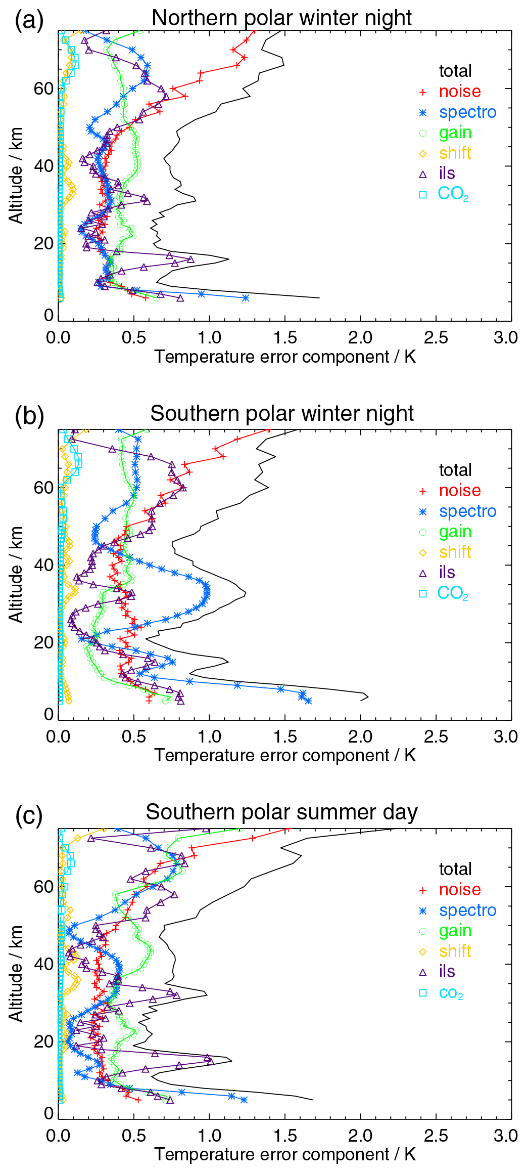
Figure 1RR data temperature error budget for northern polar winter night (a), southern polar winter night (b), and polar summer day (c) atmospheres. All error estimates are 1-σ uncertainties. Error contributions are marked “spectro” for spectroscopic error, “gain” for gain calibration error, “shift” for spectral shift error, “ils” for instrument line shape error, and “co2” for error due to CO2 volume mixing ratio uncertainty.
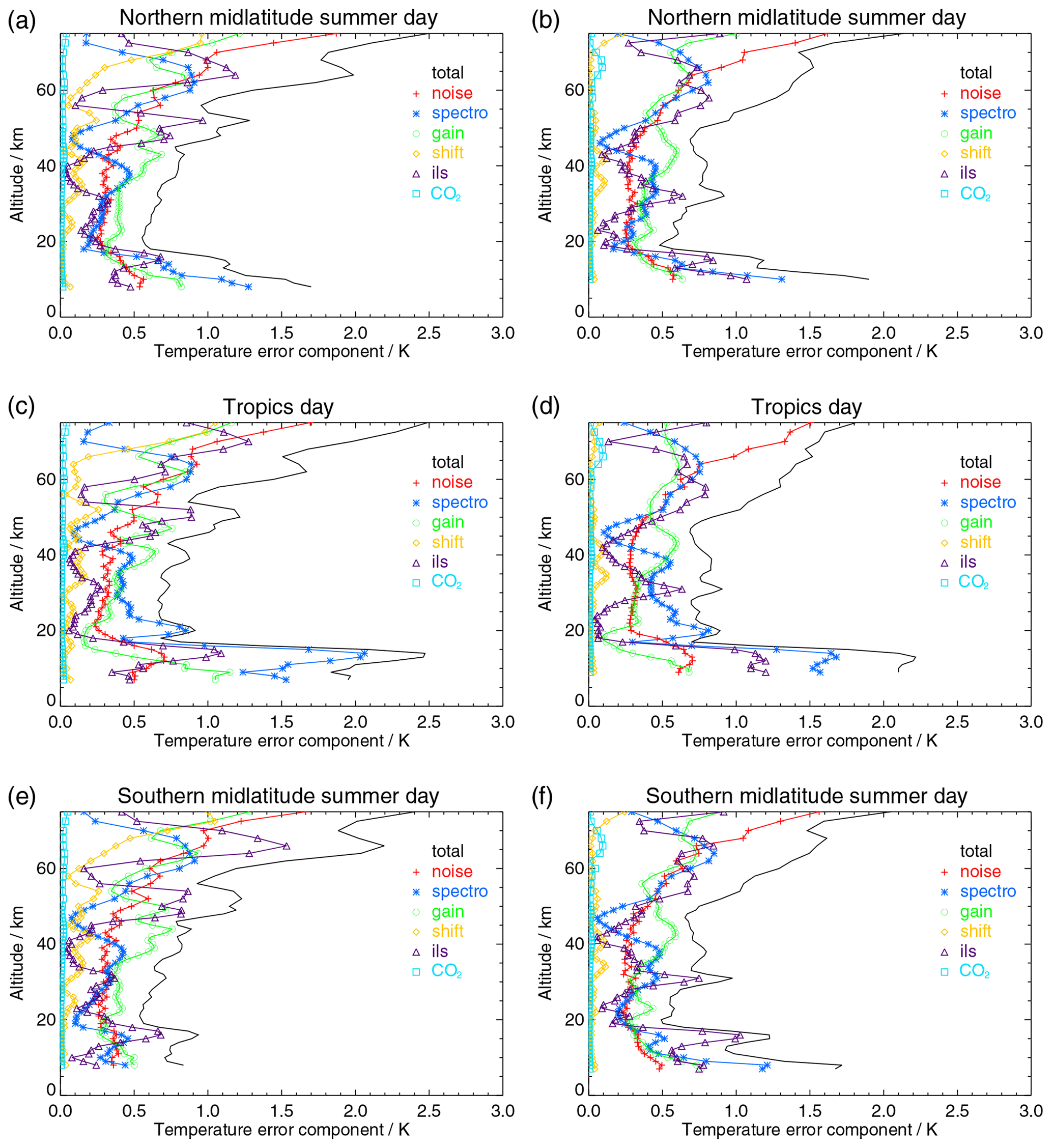
Figure 2Temperature error budget for FR data (a, c, e) and RR data (b, d, f) with color-coding as in Fig. 1: (a, b) northern midlatitude summer day, (c, d) tropical day, and (e, f) southern midlatitude summer day. All error estimates are 1-σ uncertainties.
The relevant sources of error are measurement noise, gain calibration, frequency calibration (spectral shift), mixing ratios of CO2, uncertainties in spectroscopic data, and the spectral line shape of the instrument. We first discuss the relevant error sources of the MIPAS temperature retrieval and report the input of assumed uncertainties of the error estimation. In order to comply with the TUNER (Towards Unified Error Reporting, von Clarmann et al., 2020) recommendations, we report uncertainties of chiefly random nature and systematic nature separately (Sect. 4.2 and 4.3, respectively). All reported uncertainties are standard deviations (1σ).
Every single profile retrieval comes with a noise estimate, while parameter errors, model errors, and so forth are provided as mean uncertainties for corresponding representative atmospheric conditions. The range of the total estimated error is 0.5–1.3 K in the stratosphere, with only few altitudes showing values above 1 K.
In general the uncertainties are small in the lower stratosphere and then slowly increase towards higher altitudes (see Figs. 1–2). They also increase towards the tropopause region and exhibit a strong increase below. This explains, together with the variation of the tropopause altitude, why errors for a given altitude in the tropopause region were found to vary largely between different limb scans. The retrieval proves to be particularly susceptible to errors just above the lowermost tangent altitude used. This behavior is also seen in Fig. 3, which shows the propagation of measurement noise into the retrieved temperatures. High uncertainties are found just above the lowermost tangent altitude used (solid red line). The implication for the data user is that error estimates in the tropopause region can be regarded as fairly reliable in a statistical sense but can deviate for single profiles as described above.

Figure 3The noise component of temperature error in Kelvin for sample orbit 29031 as a function of latitude and altitude. The red line is the lower edge of the instrumental field of view at the lowermost tangent altitude used. Temperatures retrieved below this altitude are solely determined by the retrieval constraint. The symbols just above the latitude axis indicate the position of the measurement and give the illumination conditions (cross: night; plus: day).
4.1 Error sources
Following the terminology of von Clarmann et al. (2020), we distinguish measurement errors, parameter errors, and model errors. Measurement errors include measurement noise and all uncertainties related to less than perfect knowledge of the instrument state. Parameter errors are uncertainties of atmospheric state parameters which are assumed to be sufficiently well known and thus not treated as unknowns of the retrieval. Model errors include deficiencies in the way the radiative transfer model describes radiative transfer through the atmosphere and uncertainties in constants such as spectroscopic data. We consider all error sources as independent from each other and thus add them quadratically to obtain the total error. We do not evaluate the smoothing error because we conceive the retrieval as an estimate of the smoothed true state rather than a smoothed estimate of the true state (see, Rodgers, 2000, Sect. 3.2.1, for a discussion of this issue). Furthermore, we provide information on error correlations in various domains (Sect. 4.4) and averaging kernels (Sect. 5.1).
4.1.1 Measurement errors
The following measurement errors were found to make a sizable contribution to the overall error budget: measurement noise, gain calibration error, instrument line shape uncertainty, and frequency calibration (spectral shift) uncertainties. Error propagation was performed using linear theory, applied to forward radiative transfer. The propagation of measurement noise was evaluated by means of Eq. (20) of von Clarmann et al. (2020), while the propagation of other measurement errors was estimated on the basis of sensitivity studies for the given atmospheric conditions.
Measurement noise, as estimated from the imaginary part of the spectra, is reported in the level-1b data. In the spectral region used for the temperature retrievals, values are in the range 15–33 nW (cm2 sr cm−1)−1 after apodization.
Gain uncertainties were adopted from Table 3 of Kleinert et al. (2018) and transformed to 1-sigma uncertainties, which gives 1.2 %. For the instrument line shape errors we used the estimates of modulation loss through self-apodization and its uncertainties, as presented by Hase (2003).
Although a spectral shift correction is carried out in a step preceding the combined temperature and pointing retrieval (see Sect. 3.2), a residual frequency calibration error is considered. It is estimated as the root-mean-square difference between the obtained frequency corrections from the shift retrievals and the linear regression line of these spectral shifts over wavenumber. The resulting uncertainty is 0.00029 cm−1.
Uncertainties in pointing and radiance offset (zero calibration) were not explicitly considered in the error estimation because these quantities were simultaneously retrieved with temperature.
4.1.2 Parameter errors
During the temperature retrieval, the concentrations of all interfering gases except O3 and H2O are assumed to be known and treated as parameters. In preceding MIPAS retrievals, climatological distributions of these interfering gases were used for this purpose. Accordingly, the climatological variability determined the uncertainty. For MIPAS version 8 retrievals, results from preceding MIPAS data processing were already available and could be used as estimates of the actual concentrations. The respective uncertainties reduce to the uncertainties of the preceding retrieval. Resulting temperature uncertainties are below 0.1 K for all interfering species that were not jointly fitted.
Since CO2 lines are used for the temperature retrieval, results are deemed particularly sensitive to the assumed CO2 mixing ratios. These were taken from the WACCM4 runs described in Sect. 3.4. Respective estimated 1-σ uncertainties are reported in Table 3. In the troposphere and stratosphere, these are based on considerations of CO2 uncertainties according to the IPCC Fifth Assessment Report and uncertainties due the seasonal variability of CO2. Above the middle mesosphere, they were estimated following comparisons between WACCM CO2 and measurements from space, mainly SABER and ACE, as shown in López-Puertas et al. (2017).
4.1.3 Model errors
Since the true atmospheric radiative transfer is not known, genuine model deficiencies could not be quantified. However, past model intercomparisons (von Clarmann et al., 2001, 2003b; Tjemkes et al., 2003; Schreier et al., 2018) do not hint at any obvious malfunction. Numerical accuracy has been tuned to a degree that corresponding temperature errors are insignificant compared to the leading error sources. The most problematic error source in the category of model errors is the uncertainty of spectroscopic data.
The uncertainty estimates can vary considerably, and it is not always clear what they represent. Additionally there is little information available as to whether the uncertainties of different spectral lines and/or bands are correlated or not. After consultation by a laboratory spectroscopist (Manfred Birk, personal communication, February 2020), we use the following 1-σ uncertainty estimates: CO2 line intensities: 1 %; pressure broadening coefficients: 2 %; exponent for temperature dependence: 0.2 (absolute).
We further assume that these uncertainties are fully correlated between different lines. We concede that these assumptions can be challenged. However, since we report the temperature uncertainties caused by spectroscopic uncertainties separately, data users endowed with a different degree of optimism can easily rescale the resulting error estimates. Uncertainty estimates provided along with the spectroscopic data compilation by Flaud et al. (2003) appear to be less optimistic than ours. However, preliminary validation do not support the resulting larger temperature bias.
For former MIPAS temperature data, uncertainties due to the neglect of non-local thermodynamic equilibrium and unaccounted horizontal variability of the atmospheric state were reported. These error sources are not considered here because nonlinear thermodynamic equilibrium effects and the horizontally varying atmosphere are explicitly modeled (see Sect. 3.11 and 3.5).
4.2 Random errors
When comparing measurements of the same state variable by two different instruments, random errors are errors that contribute to the intrinsic variability (standard deviation) of the differences. The main sources of random errors of MIPAS temperature are measurement noise, spectral shift, gain calibration uncertainties, and the uncertainties of CO2 mixing ratios. Measurement noise is random by nature. Spectral shift originally has a more systematic characteristic, but the residual frequency calibration error after correction is random. According to our definition, gain calibration uncertainties are also random. While they are obviously systematic within one gain calibration period, they contribute in the long run rather to the standard deviation of differences between measurement systems than to the bias. Similar considerations apply to the uncertainties in CO2 mixing ratios, which we consider as random, although they are presumably positively correlated among subsequent measurements. The adequacy of this classification of uncertainties in random and systematic components will be critically tested in a dedicated validation study. None of the other random error components, e.g., mixing ratios of interfering species, makes a sizable contribution to the error budget.
For most atmospheric conditions and altitudes, the random temperature uncertainty varies between 0.4 and 1 K. Occasional excursions up to 1.3 K are encountered above 60 km altitude (Tables A1–A9 and Figs. 1–2).
As a rule of thumb, measurement noise is – everything else unchanged – larger for colder and smaller for warmer atmospheres. For the other random error components, no such simple dependence of the error on the atmospheric state can be provided.
For some applications the error covariances are relevant. These depend both on the structure of the Jacobian of the inverse problem and on the covariances of the ingoing uncertainties. While it is hard to fully quantify the latter, we present a sample error correlation matrix that characterizes the former in the Appendix (Table B1). The correlation matrix allows the construction of an approximate covariance matrix for any given retrieval noise.
4.3 Systematic errors
Systematic errors are, regardless of their origin, errors which explain the bias between measurements of the same state variable by different instruments observing the same part of the atmosphere. The main sources of systematic error in MIPAS temperatures below the mid-mesosphere are uncertainties in spectroscopic data and instrument line shape uncertainties. To classify these as systematic is admittedly an idealization because the actual conditions will somehow modulate the actual resulting errors; e.g., the impact of the uncertainty of the line intensity of an interfering gas depends on the abundance of the interfering species, which may vary randomly. Since, however, the CO2 lines chosen for the temperature retrieval are strong lines and only weakly interfered by transitions of other species, this random modulation of systematic errors is deemed negligible and the classification of related temperature uncertainties as chiefly systematic seems justified.
The other source of systematic error in MIPAS temperatures is uncertainties in the instrument line shape. Since the same set of coefficients is used for all measurements, this error is clearly systematic in nature. However, it must be kept in mind that modulations of the related initially systematic error by the variable sensitivity of the retrieval that depends on the actual state of the atmosphere will generate a certain random component.
In all altitudes except the uppermost ones, the error budget is dominated by these systematic errors. With this in mind, it can be considered a particularly grave deficit that uncertainties in spectroscopic data are so vaguely characterized with respect to their confidence limits and correlation characteristics.
4.4 Error correlations in various domains
Since our retrieval decomposes the inverse problem profile by profile, vertical correlations of measurement noise are represented by the respective covariance matrix. Related correlation coefficients are represented in Table B1. Errors due to spectral shift are expected to be almost fully correlated in the altitude domain because the frequency calibration correction is performed individually for entire limb scans. Since frequency calibration corrections are constrained towards the long-term mean, a positive error correlation in the time domain also has to be expected.
As stated above, positive correlations are expected for gain calibration errors of measurements recorded within one gain calibration period. This leads to positive error correlations in altitude and between subsequent limb scans. The typical length of a gain calibration period is 1 d and occasionally 2 d. Errors due to uncertain mixing ratios of CO2 are also expected to be correlated in altitude and between subsequent limb scans. Correlation lengths depend on the actual spatial and temporal extension of the CO2 anomalies.
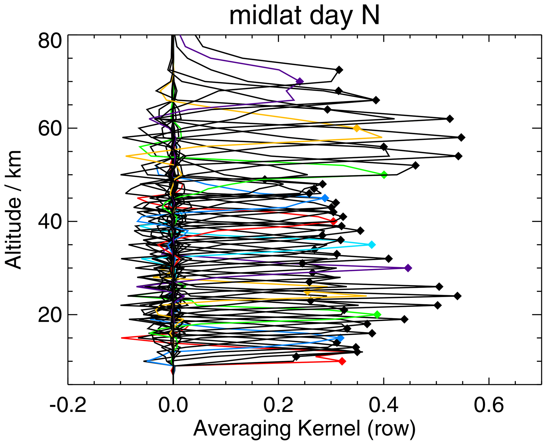
Figure 4MIPAS temperature averaging kernels for a northern midlatitude daytime observation. For clarity, the kernels belonging to retrieval altitudes 10, 15, 20 … km are color-coded. Diamonds represent the nominal altitudes.
5.1 Averaging kernels and vertical resolution
The vertical resolution of the temperature profiles, estimated as the full width at half maximum of the respective row of the averaging kernel matrix, varies around 3 km in the altitude range up to 40 km (Fig. 4). Above, it gradually deteriorates towards 7 km at 70 km. A local maximum of vertical resolution values of approx. 3.3 km is typically found at the tropical tropopause layer (around 15 km altitude) and is attributed to particularly low temperatures. The actual values of the vertical resolution are provided for each limb scan along with the data on the MIPAS data server (http://www.imk-asf.kit.edu/english/308.php, last access: 21 May 2021).
The averaging kernels are generally well behaved in the sense that they peak at their nominal altitude. That is to say, the temperature retrieval at altitude z is most sensitive to the true temperature at altitude z. Further, the kernels are fairly symmetric. This rules out major information displacement by the retrieval. The pronounced side-wiggles are a typical feature of a retrieval on a grid that is much finer than the measurement grid. This does not point at a weakness of the retrieval setup. Instead, the often smoother averaging kernels of retrievals on coarser retrieval grids just do not represent these features because the Jacobians do not resolve them. Understanding the column of an averaging kernel matrix as the response of the retrieval to a delta perturbation of the true profile, the so-called delta perturbation on a coarse grid perturbs a much wider part of the atmosphere and thus is not comparable to our fine-grid averaging kernels.
5.2 Temperature differences with respect to previous data versions
Preceding versions of MIPAS temperature data were already quite a mature and well-validated data product (e.g. Wang et al., 2004, 2005). It has already been shown that MIPAS sees the expected temperature features in the middle atmosphere (e.g., von Clarmann et al., 2009b). Thus, it does not come as a surprise that, for most parts of the atmosphere, the differences between the new improved temperature data and the previous ones are small. (Fig. 5). Only near the stratopause and above are major differences observed. These are attributed to the use of the extended set of microwindows (see Sect. 3.6) and to the new WACCM-based prior information (see Sect. 3.4), which is expected to represent the actual conditions much better than the climatology used previously.
In this section we concentrate on improvements with respect to the previous data version for cases where problems with the older data had already been identified, and we investigate to which degree MIPAS provides additional information with respect to pre-existing knowledge on temperature and line-of-sight pointing.
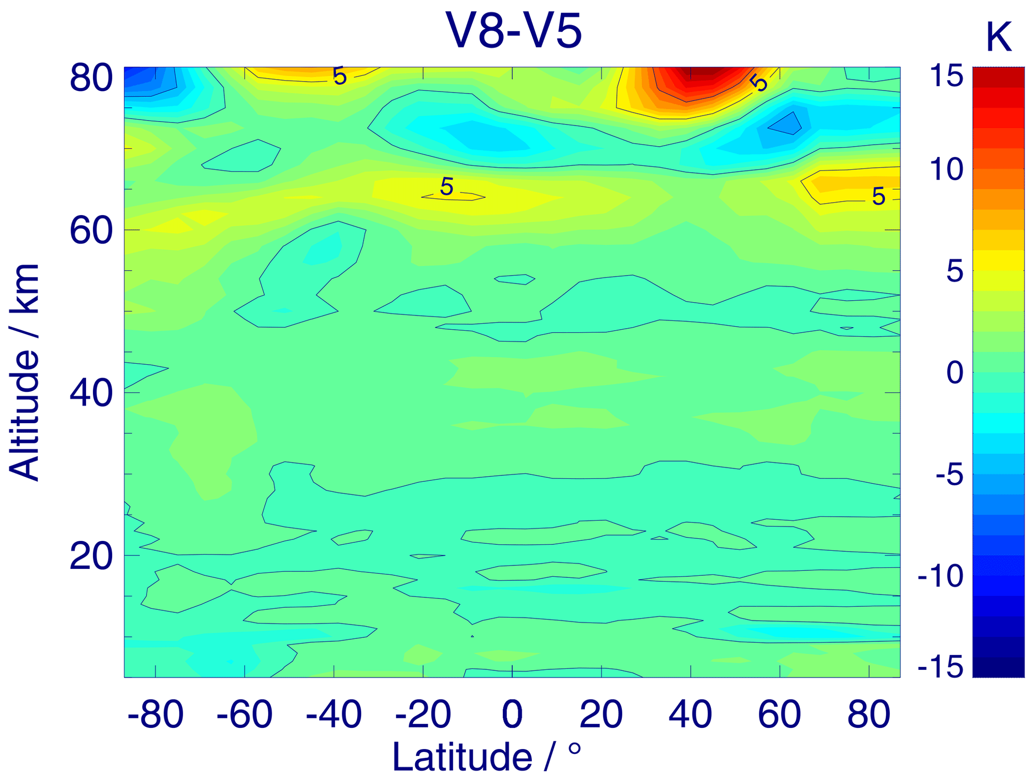
Figure 5Mean monthly MIPAS temperature differences between version V8R_T_261 and V5R_T_220 for August 2010.
5.2.1 Drifts
The technical aspects of the drifts in MIPAS data due to detector aging have already been discussed in Sect. 2. Here we assess to which degree the revised nonlinearity correction in the level-1b processing was successful in reducing related drifts in temperature. Fig. 6 shows the drift of MIPAS V5 temperature relative to the microwave radiometer AMSU (advanced microwave sounding unit) and to the infrared radiometer SSU (stratospheric sounding unit), according to Fig. 9 of McLandress et al. (2015). Since their Fig. 9 also shows the temperature drift between the microwave limb sounder Aura MLS (microwave limb sounder) and AMSU and SSU to be very small, we believe the AMSU and SSU reference to be a reasonably reliable one for a tentative temperature drift assessment.
In Fig. 6 all altitudes exhibit a negative temperature drift between MIPAS V5 and AMSU and SSU (solid black and red lines, respectively). Between 15 and 25 km this negative drift is roughly constant at −0.2 K per decade, but becomes more negative with altitude to reach approx. −0.9 K per decade at 40–45 km.
To assess the quality of the new MIPAS V8 data product, we calculated the temperature drift of MIPAS V5 relative to MIPAS V8. We tried to come as close as possible to the drift calculation method of McLandress et al. (2015): we average over the same latitude range from 75∘ S to 75∘ N, use the same time range from 2004 to 2012, and take into account the respective AMSU and SSU altitudes and altitude weightings by averaging over altitude ranges corresponding to the full width at half maximum of the respective weighting functions (gained from Fig. 1 of McLandress et al., 2015). The MIPAS V5 minus V8 drift values are shown as broken lines with diamond symbols in Fig. 6. If the V8 temperature data showed the same trend as AMSU and SSU, one would expect this V5 minus V8 drift curves to essentially fall on top of the V5 minus AMSU and SSU curves.
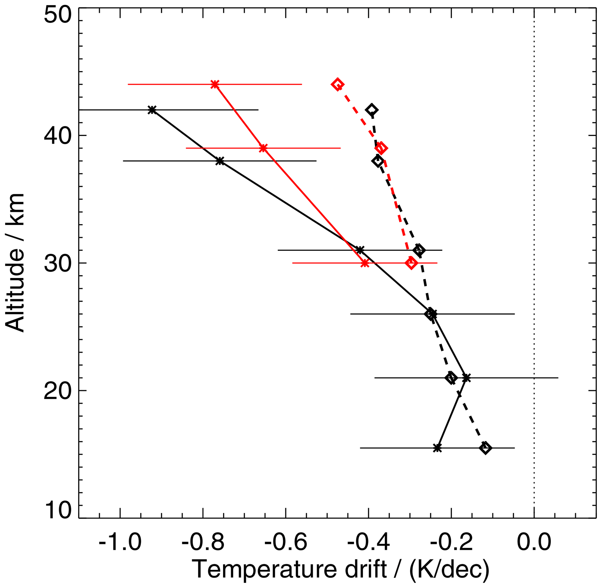
Figure 6Temperature drift between MIPAS V5 and AMSU (solid black line) and MIPAS V5 and SSU (solid red line) data in the sense MIPAS V5 minus the reference unit (AMSU, SSU). Error bars are 1σ. Data are based on Fig. 9 of McLandress et al. (2015). Broken lines with diamond symbols show the drift between MIPAS V5 and V8 temperatures. Altitudes, time range, and averaging were chosen according to the calculations of McLandress et al. (2015). See the text for details.
This is indeed the case for altitudes between 15 and 30 km. Here the MIPAS drift is completely corrected by the revised V8 nonlinearity-corrected calibration. Above 25 km, the negative drift between MIPAS V5 and V8 is less pronounced than the drifts between MIPAS V5 and AMSU and SSU. This means that the new nonlinearity-corrected calibration removes the MIPAS drift only partly and that V8 still seems to have a negative temperature drift. At around 40 km, only half of the V5 drift is removed. However, since at all covered altitude levels the observed drift is less pronounced in V8 than in V5, and since the drift is, within the error bars, fully removed below 30 km, the revised nonlinearity treatment in the calibration of the V8 level-1b data seems to work considerably better than that used in the V5 calibration.
5.2.2 Consistency between high-resolution and reduced-resolution results
In time series of MIPAS V5 data products, jumps in atmospheric state variables can be often seen between the full spectral resolution period (2002–2004) and the reduced spectral resolution period (2005–2012). Although methodical development work was never targeted at removing these jumps, as a side effect of other retrieval optimization work, the full-resolution and reduced-resolution datasets have become much better inter-consistent in the sense that these jumps are now largely reduced.
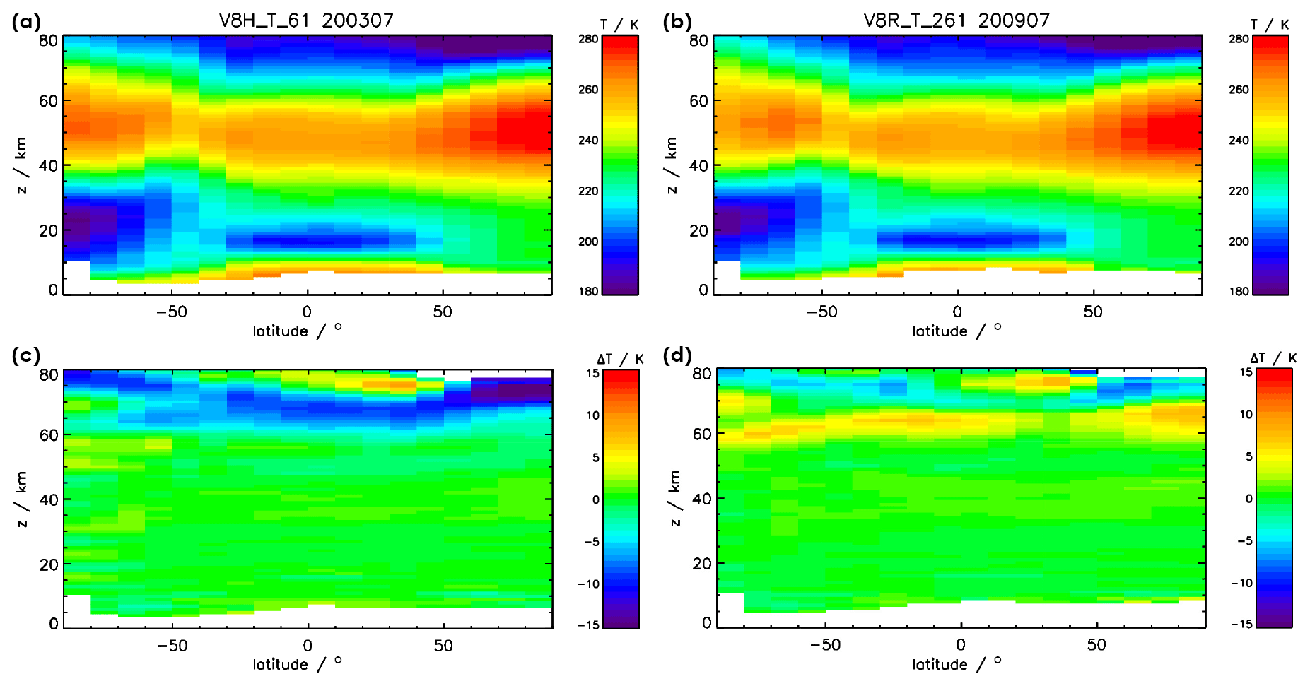
Figure 7(a, b) Monthly mean V8 temperature in 10∘ latitude bins for July 2003 (FR period, a, c) and July 2009 (RR, b, d). (c) Differences between V8 and V5 monthly mean temperatures for FR data (July 2003). (d) Differences between V8 and V5 monthly mean temperatures for RR data (July 2009).
An illustration of this inconsistency problem is given in Fig. 7. The top row shows monthly temperature means of V8 data in 10∘ bins for FR (July 2003) and RR (July 2009) data. There is no obvious inconsistency. However, the lower row of Fig. 7 shows that the differences between V8 and V5 monthly mean data clearly differ for the full-resolution data (V8 minus V5 for FR measurement period; on the lower left) and the reduced-resolution data (V8 minus V5 for RR; on the lower right).
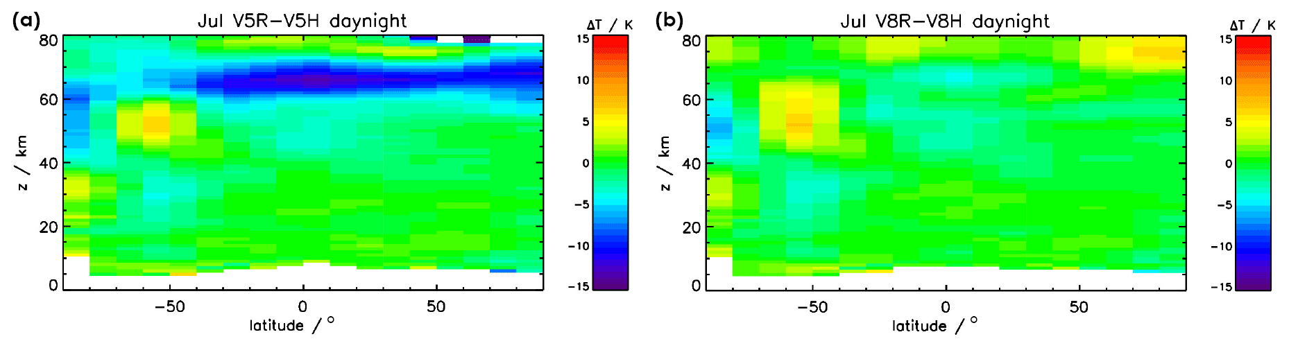
Figure 8Difference between reduced-resolution (July 2009) and full-resolution (July 2003) monthly mean data for V5 (a) and V8 (b).
To further clarify this inconsistency, the difference between reduced-resolution and full-resolution monthly mean data was calculated separately for data versions V5 and V8. From Fig. 8, it is obvious that the differences in V5 (left panel) are much more pronounced compared to those in V8. The structure of the remaining differences in V8 can also be seen in the V5 differences, suggesting that this is a real atmospheric feature, since mean temperatures of July 2009 and 2003 can be expected to differ somewhat. The result of this analysis is that our V8 data are much more consistent between the MIPAS FR and RR measurement periods than preceding data versions.
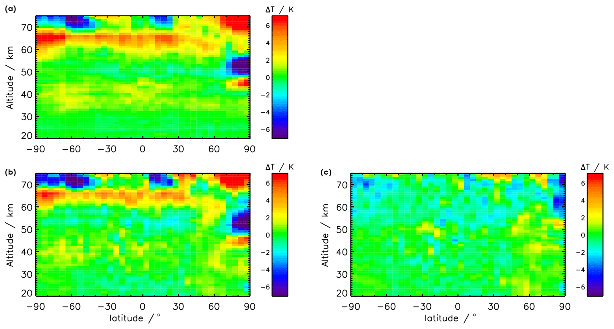
Figure 9Temperature differences for 20 February 2009. (a) V8 nominal-mode minus V5 nominal-mode data. (b) V5 middle-atmosphere mode minus V5 nominal-mode data. (c) V5 middle-atmosphere mode minus V8 nominal-mode data. Specifically, the used data versions are V5R_T_221 (NOM), V5R_T_521 (middle atmosphere), and V8R_T_261 (NOM).
5.2.3 Case study: elevated stratopause situations
The dependence of retrieved temperatures above about 60 km on the prior information is caused by the fact that MIPAS cannot resolve the shape of the temperature profile above the highest tangent altitude. This problem has motivated us to replace the climatological NRLMSISE-00-based prior information at these altitudes with prior information from a debiased specified dynamics WACCM run (see, Sect. 3.4). As a test case, an elevated stratopause event in February 2009 was chosen. A discussion of this episode and independent evidence of this event are reported, e.g., in Funke et al. (2017). The onset of this event was at the beginning of February, and in the second half of February the temperature anomaly reached altitudes relevant to MIPAS retrievals.
For 20 February 2009, the difference between V8 and V5 nominal-mode temperature data is shown in the top left panel of (V5 NOM data are V5_T_221). Additionally, the differences between V5 middle-atmosphere mode and V5 NOM data (lower left panel) and between V5 middle-atmosphere mode and V8 NOM data (lower right panel) are depicted in Fig. 9. If we take the V5 middle-atmosphere data as reference, which are based on measurements from 18–102 km (for a validation study of this data see García-Comas et al., 2014), it is clear that the V8 NOM data give a much better picture of the temperature above 60 km and also of temperatures under polar winter conditions.
The different behavior of the nominal-mode retrievals is evident. Globally, differences in the data versions are confined to altitudes above 60 km and occasionally exceed 5 K. Here the positive temperature differences hint at too low temperatures in version 5 even at altitudes where MIPAS has measurement information. This is a result of error correlations with altitudes above about 68 km where the retrieval has to rely on the shape of the a priori profile. The too low temperatures in V5 (showing up as positive differences V8–V5) compensate the too high a priori-driven temperatures above 70 km to best fit the measured radiance signal.
At northern polar latitudes the inclusion of the new a priori information, which better reflects the actual conditions, is more drastic. The warm region above 70 km is not represented by the V5 NRLMSISE-00-based a priori, and this error propagates downward to 40 km, showing up as temperature oscillations with too warm temperatures in V5 (negative V8–V5 difference) around 50 km and too cold temperatures (positive V8–V5 differences) around 42 km altitude. In summary, the new data version better represents this event not only at altitudes above the uppermost tangent altitude (around 68 km) but also below because the inadequate temperature profile above the uppermost tangent altitude in V5_T_221 triggered, via error correlations, temperature errors also at altitudes where MIPAS is able to resolve the temperature profile.
5.3 Case study on differences with respect to ECMWF temperatures: temperature waves
MIPAS is able to reveal structures in temperature profiles independently of the a priori information. We demonstrate this by using two examples of features in temperature profiles that might be attributed to gravity waves. In the left-hand panels of Fig. 10, temperature profiles for MIPAS retrievals (black lines) and the corresponding ECMWF-based a priori (red lines) are shown, while the right-hand panels show the differences between temperature profile minus the respective vertically smoothed temperature profile for retrieval and a priori data. Smoothing is done with a boxcar of 10 km width.
We rule out that the retrieved wave structure is a numerical artifact of the retrieval caused by too weak regularization because the MIPAS result agrees well with the ECMWF ERA-interim analysis, which shows very similar structure. The upper panels in Fig. 10 show an example. The example shown in the lower panel demonstrates that MIPAS is able to retrieve such structures independently from the a priori information. There (as in many other cases) we find wave structures in both datasets (MIPAS and ECMWF analyses) with similar vertical wavelengths but different phases. The retrieval scheme chosen does not employ any mechanism that would be able to map a vertically shifted structure in the prior information onto the result. Therefore, these results prove that structures in vertical profiles, and in particular these wave structures, are independent MIPAS measurement information.
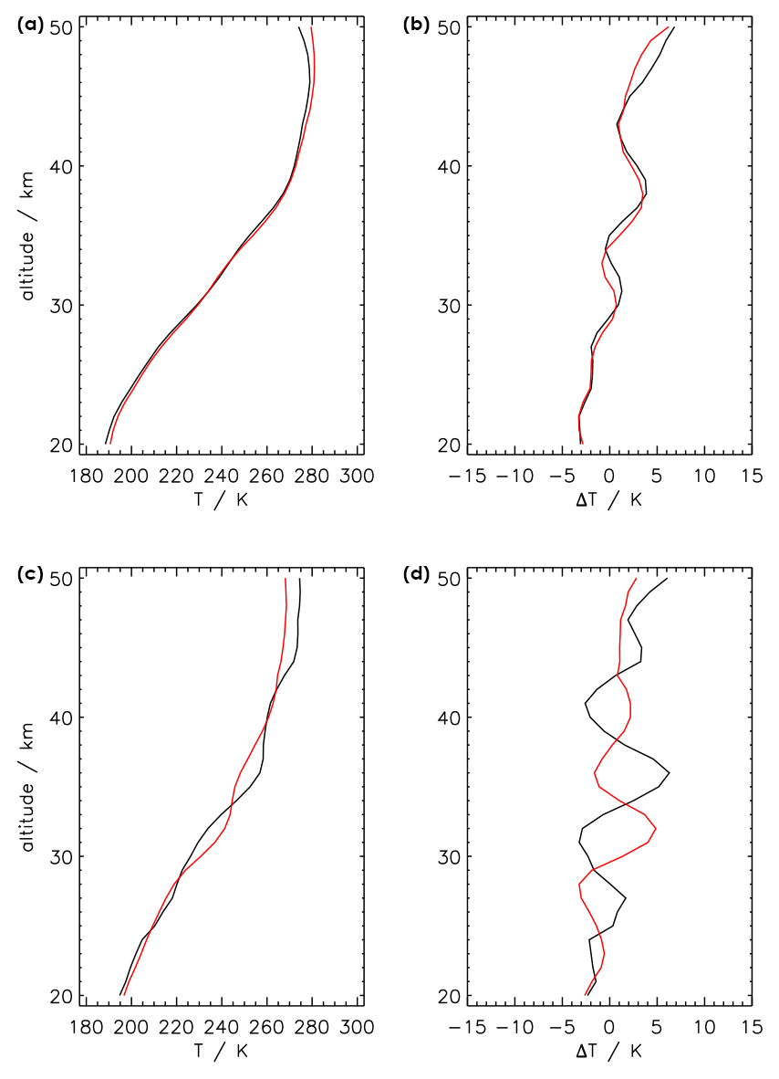
Figure 10(a, c) ECMWF ERA-Interim (red) and retrieved (black) temperature profile at 67.3∘ S, 32.5∘ W on 24 September 2009 (a, b) and at 62.0∘ S, 5.6∘ W on 5 September 2009 (c, d). (b, d) Differences in profiles, with a smoothed version of the profiles in the left panels, obtained with a boxcar smoothing of 10 km width, displaying the wave structure of the original profiles. MIPAS and ECMWF profiles agree well with respect to the wavelength and amplitude of the temperature waves but not always with respect to the phase.
5.4 Pointing differences with respect to level-1b engineering information
Contrary to other MIPAS data processors (Dinelli et al., 2010, Raspollini et al., 2013, and http://eodg.atm.ox.ac.uk/MORSE/, last access: 21 May 2021), the IMK/IAA processor retrieves the pointing information in terms of tangent altitudes from the spectra (see Sect. 2.2 of von Clarmann et al., 2003a), using the engineering information only as a Bayesian constraint and not as a hard constraint (see Sect. 3.3). The comparison between the retrieved data and the level-1b engineering information has been used in the past to characterize the MIPAS pointing and to improve the algorithm involved in the calculation of the line of sight (Kiefer et al., 2007). Meanwhile, several improvements of this algorithm have been implemented, and now the comparison reveals the following information.
-
The engineering information on the tangent altitudes has changed in a noticeable manner between data versions V5 and V8. Mean changes between engineering tangent altitudes can reach and exceed 600 m at most altitudes for FR data and −400 m for the RR period (signs according to V5 minus V8). The impact of the inclusion of atmospheric refraction in the calculation of the engineering tangent altitudes for level-1b versions after V5 is clearly visible as a difference below 20 km.
-
Mean differences in retrieved tangent altitudes (V5 minus V8) vary between −100 and 100 m at altitudes below 35 km and steadily increase above to values of 600 m at 60 km altitude for FR data. For the RR period, these differences vary between −100 and 100 m over the entire altitude range.
-
Altitude-averaged differences between engineering tangent altitudes and retrieved tangent altitudes are largest for data version V5. They vary around 400 m in large parts of the altitude range for the FR period and around −370 m for the RR data. For version V8, the differences are around −100 m for FR and −310 m for RR data. The standard deviations of these differences between engineering tangent altitudes and retrieved tangent altitudes were reduced between V5 and V8 data from 450 to 150 m for FR and from 250 to 160 m for RR. This suggests that the engineering tangent altitudes have improved considerably over the earlier versions.
-
The course with altitude of the differences between engineering tangent altitudes and retrieved tangent altitudes for V8 data shows that for both the FR and RR period there is a steady increase of 200 m between the lowest altitudes and approx. 20 km. Above this point, FR differences further increase by about 100 m up to 35 km and from there on increase less than 100 m up to 60 km. The RR differences essentially stay constant between 20 and 60 km.
-
No discernable latitude dependence was found in these differences. This means that the error source which lead to the latitude-dependent differences identified in Kiefer et al. (2007) has been successfully corrected.
-
Also these findings confirm that quite independent tangent altitude information is indeed retrieved by the IMK/IAA MIPAS processor and that the retrieval is not over-constrained toward the engineering information.
In summary, the retrieval vector of the IMK/IAA temperature retrieval contains, besides the temperature profile, (i) linear horizontal gradients in latitude and longitude directions, (ii) tangent altitudes of all spectra of the limb scan under analysis, (iii–iv) vertical profiles of O3 and H2O mixing ratios, (v) a vertical profile of background continuum emission per microwindow, and (vi) a radiance offset correction for each microwindow and each tangent altitude. Beyond new level-1b radiance spectra, improvements with respect to older data versions refer to the following upgrades of the retrieval scheme. The frequency calibration correction scheme is made more robust. Additional microwindows were included to obtain more information from high altitudes. A non-LTE parameterization that accounts for the temperature dependence of vibrational non-LTE populations in an approximate manner has been adopted. Better temperature a priori information is used for higher altitudes, taking the actual conditions better into account. Trace gas mixing ratios from previous MIPAS data versions are used to model the contributions of interfering species. An empirical background continuum is retrieved to altitudes up to 58 km instead of only 32 km. An improved offset calibration correction has been used. Due to their significant contribution to the signal in CO2 microwindows, mixing ratios of O3 and H2O were jointly fitted. Forward calculations were based on updated spectroscopic data. A TUNER-compliant error budget is provided and random, systematic, and total error components are included in the V8 data product.
The developments described above led to the following improvements in the MIPAS temperature data. The drift caused by the nonlinearity correction applied in the course of the radiance calibration has been reduced. Results from the high spectral resolution period (2002–2004) and the reduced spectral resolution period (2005–2012) are now more consistent. Temperature profiles for situations where the temperature profile above the altitude range covered by MIPAS tangent altitudes deviates strongly from the climatological mean, e.g., elevated stratopause situations, are now much more realistic. Compared to previous data versions, a larger fraction of the retrievals converged. We have shown that although ECMWF ERA-Interim temperature fields are used to constrain the temperature retrievals, vertical temperature wave information can be retrieved that is independent of the prior information used.
The further evaluation of MIPAS version 8 temperatures is deferred to a dedicated validation study. This work is confined to measurements recorded in nominal and UTLS measurement modes. The temperature retrieval from spectra recorded in the middle- and upper-atmospheric measurement modes are reported in a companion paper by García-Comas et al. (2021).
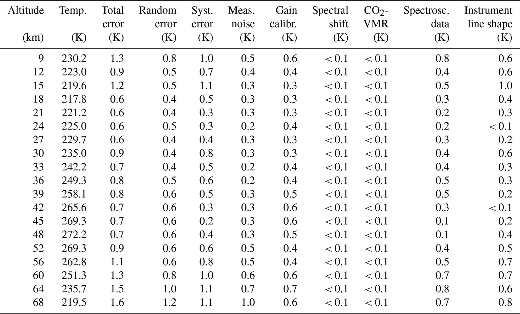
The error budget of MIPAS temperatures for some representative atmospheric conditions is reported in Tables A1–A9. The atmospheric conditions under consideration are northern and southern polar winter night, southern polar summer day, northern and southern midlatitudes during the day and at night, and tropical day and night. The lowest altitude for which errors are given obviously depends on the atmospheric condition. There are two reasons for this. First, the lowest altitude of MIPAS nominal-mode observations varies with latitude, with the lowest tangent altitude of one measurement location being 5 km at the poles and 12 km at the Equator. The second and more important factor is that the errors are only defined at altitudes where the spectra are not contaminated by IR emission of clouds. Since the cloud altitude strongly depends on latitude and season (e.g., equatorial convection, polar winter polar stratospheric clouds), a variation in the lowest altitude is observed.
The complete error estimates for day and night of spring, summer, autumn, and winter conditions at polar and middle latitudes, as well as for the tropics, are presented in the Supplement.
Table A1RR data temperature error budget for northern polar winter night. All uncertainties are 1σ.
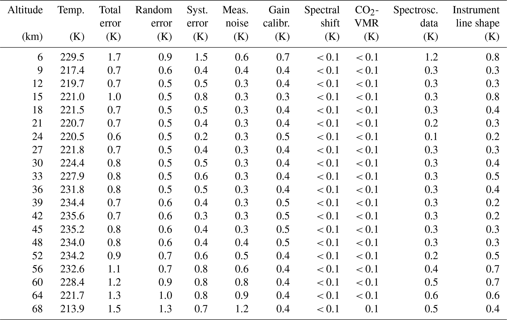
Table A2RR data temperature error budget for southern polar winter night. All uncertainties are 1σ.
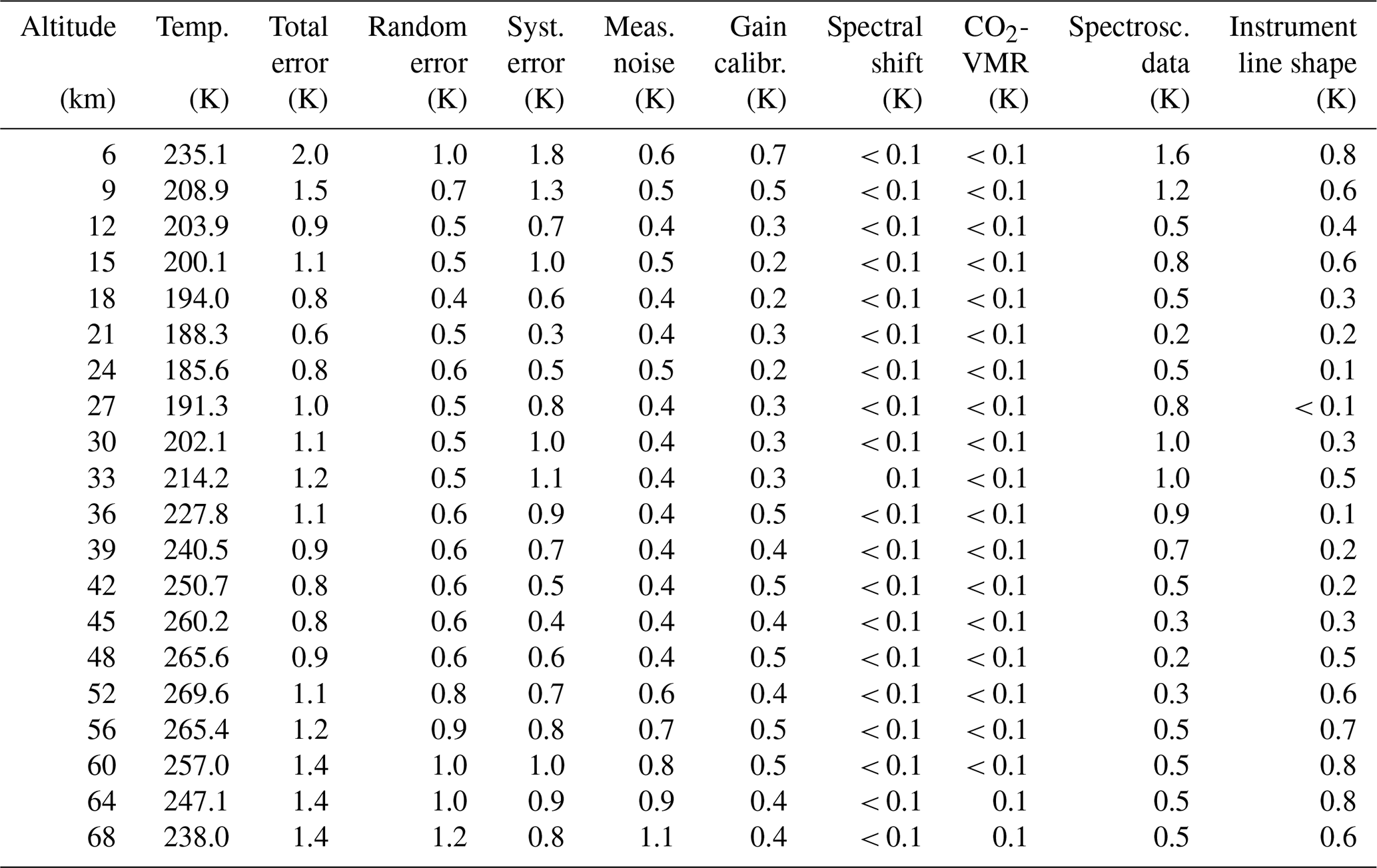
Table A3 RR data temperature error budget for southern polar summer day. All uncertainties are 1σ.
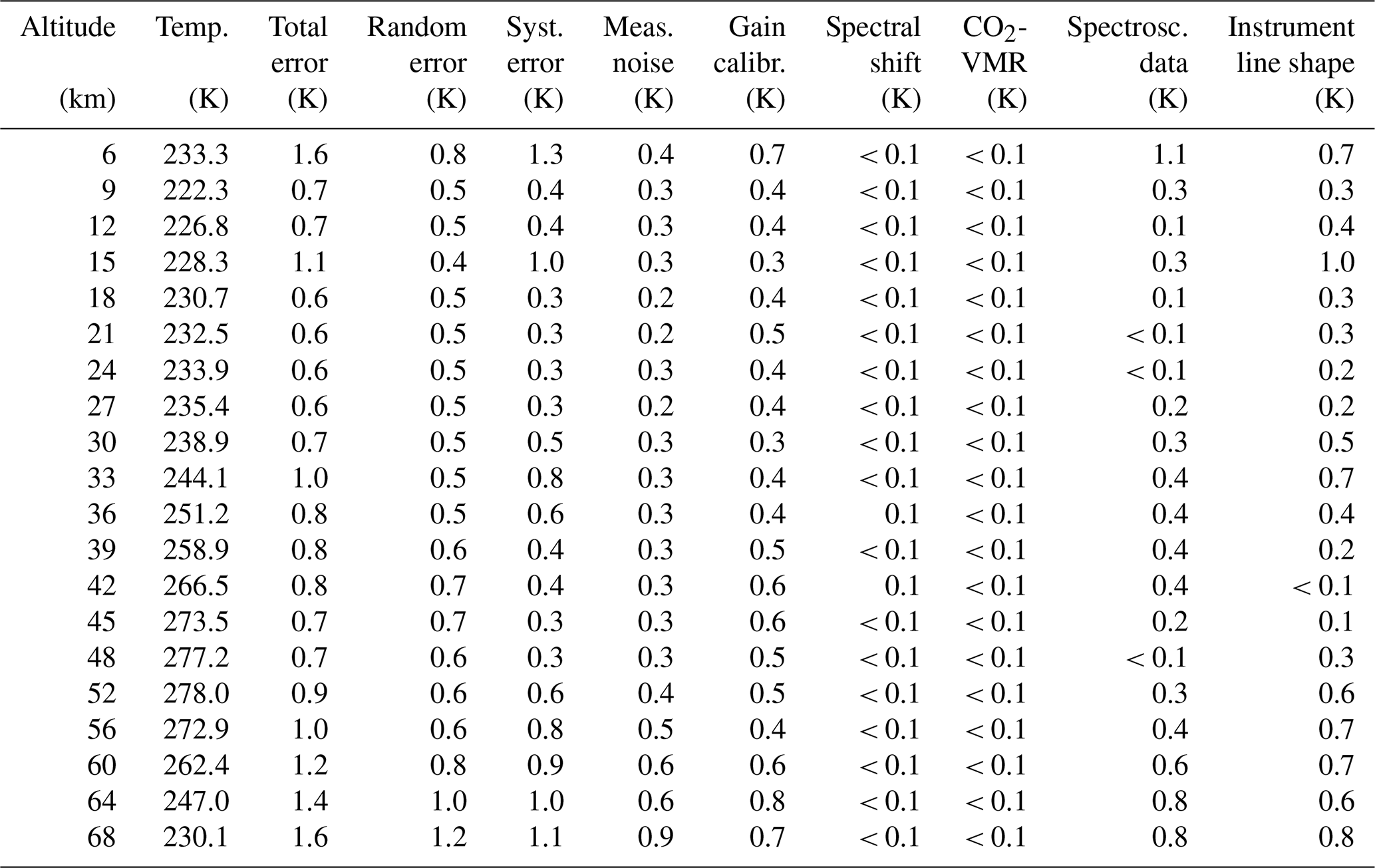
Table A4FR data temperature error budget for northern midlatitude summer day. All uncertainties are 1σ.
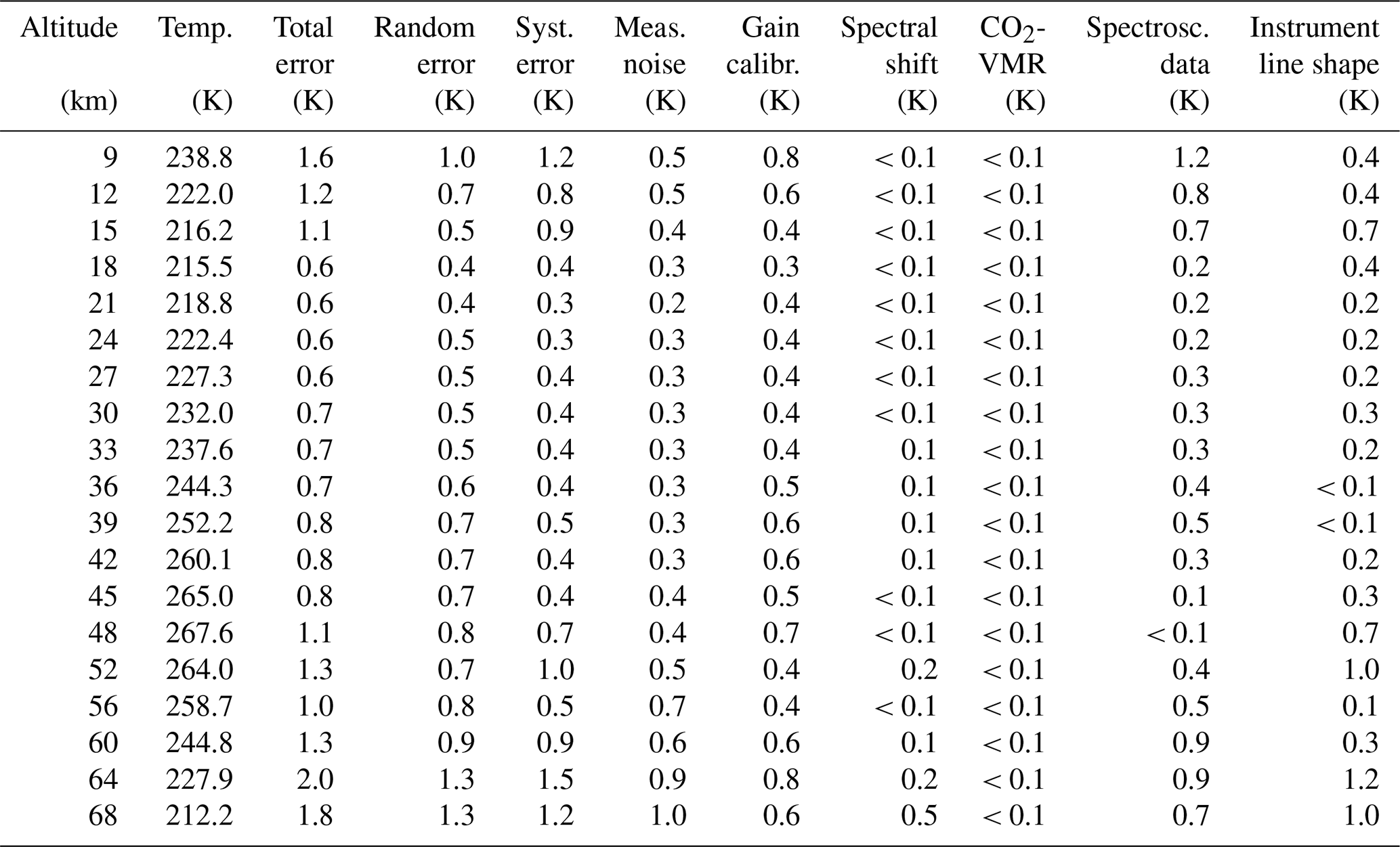
Table A5RR data temperature error budget for northern midlatitude summer day. All uncertainties are 1σ.
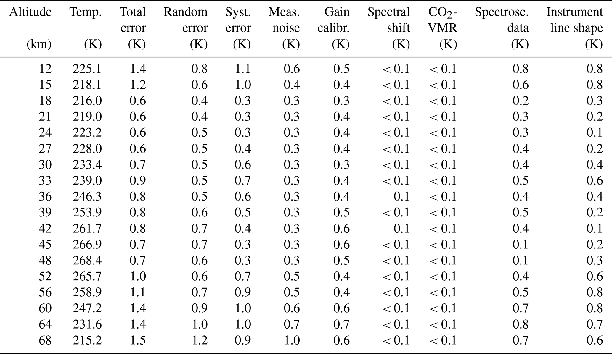
Table A6FR data temperature error budget for tropical day. All uncertainties are 1σ.

Table A7RR data temperature error budget for tropical day. All uncertainties are 1σ.
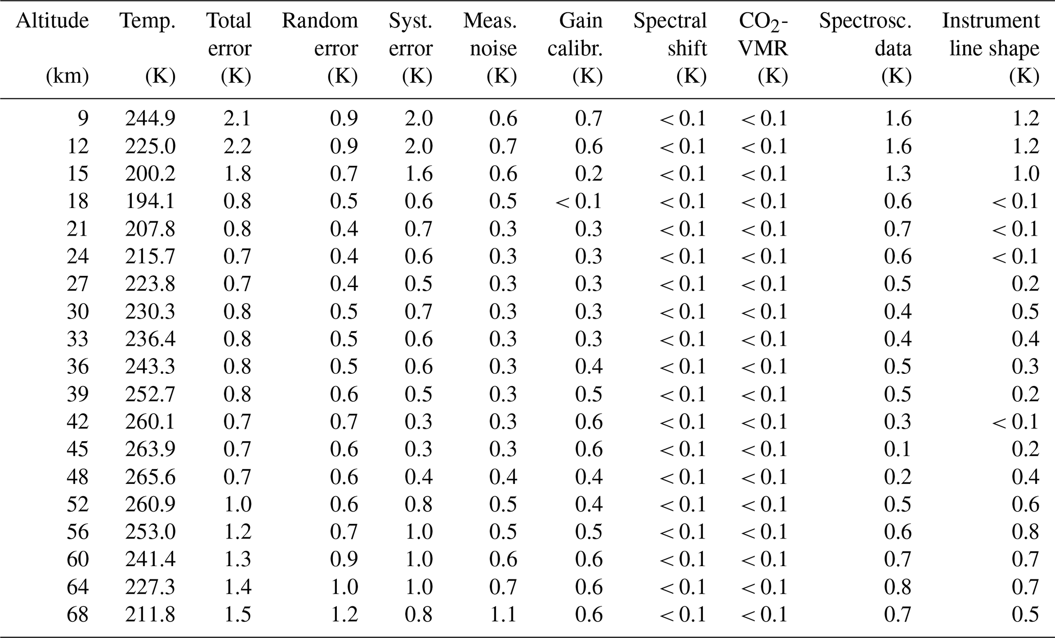
Table A8FR data temperature error budget for southern midlatitude summer day. All uncertainties are 1σ.
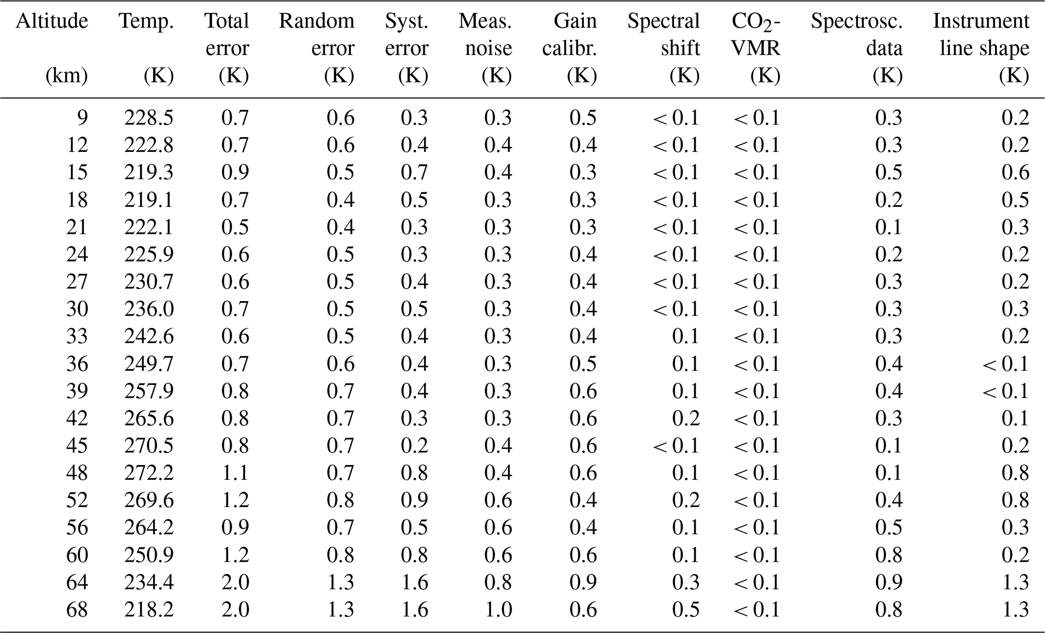
Table A9 RR data temperature error budget for southern midlatitude summer day. All uncertainties are 1σ.
For some applications the error covariances are relevant. In Table B1 we present a sample error correlation matrix. The error correlation matrix is a covariance matrix of retrieval noise divided component-wise by the proper standard deviation. The result is a matrix of correlation components that can be used to construct an approximate covariance matrix for any given retrieval noise.
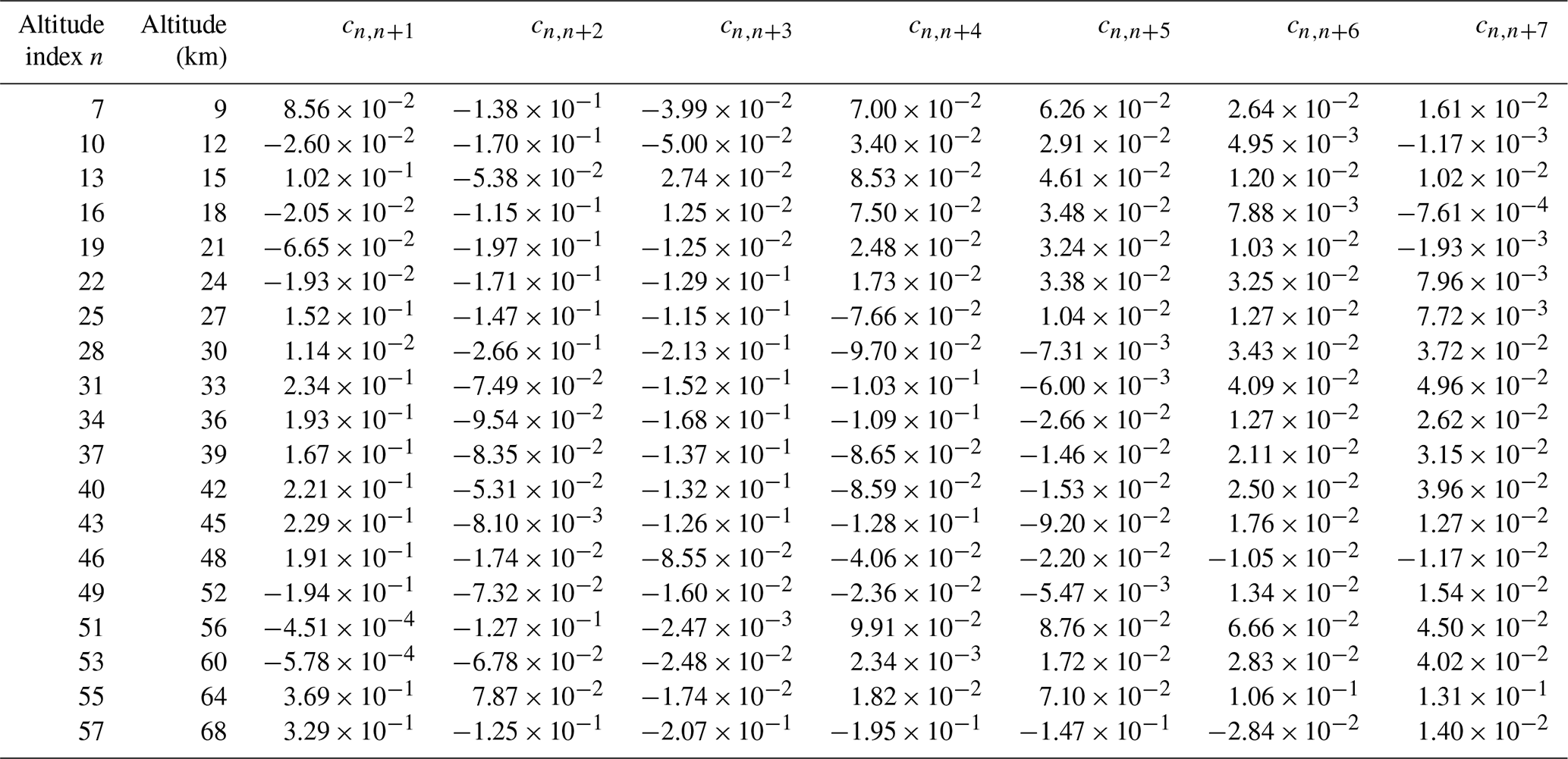
Table B1Sample MIPAS temperature noise error correlation values between adjacent retrieval altitudes for selected altitudes of a limb scan on 12 July 2009. , , etc., mark the first, second, etc., off-diagonal elements of the respective nth row of the noise error correlation matrix.
The MIPAS data can be obtained from the KITopen repository (https://doi.org/10.5445/IR/1000131913, Kiefer et al., 2021).
The supplement related to this article is available online at: https://doi.org/10.5194/amt-14-4111-2021-supplement.
Since the results presented in this paper are a team effort, the following list of author contributions is by no means comprehensive. Instead only the most prominent contributions are listed. MK developed the retrieval setup, coordinated, partly performed related test calculations, contributed graphics, and had the final editorial responsibility for this paper. TvC wrote large parts of the text, organized related discussions, and was responsible for the TUNER compliance of error estimates. BF provided the parameterized NLTE approach and implemented the updated frequency calibration and offset correction. BF, MGC, and MLP took care that the retrieval setup was developed in a way that inter-consistency with the retrieval setups of middle- and upper-atmospheric measurement modes was maintained. Furthermore, they provided the CO2 uncertainties. MLP and BF built the a priori temperature distributions from the WACCM data. NG was responsible for spectroscopy issues and error estimation calculations, carried out some of the retrieval tests, and contributed graphics. UG provided and maintained the retrieval software, including the data archive; he was also responsible for level-1b data import and quality control. SK and ALi ran the retrievals and visualized the results. SK contributed graphics. AK was responsible for L1-related issues. ALa contributed to quality control. DM provided the WACCM calculations. GPS identified issues to be solved and took care of quality control. All authors suggested solutions for various problems encountered during the development phase and critically discussed the results and the manuscript.
The authors declare that they have no conflict of interest.
This article is part of the special issue “IMK–IAA MIPAS version 8 data: retrieval, validation, and application (ACP/AMT inter-journal SI)”. It is not associated with a conference.
Spectra used for this work were provided by the European Space Agency. We would like to thank the MIPAS Quality Working Group for enlightening discussions and Claus Zehner for particularly helpful support. The computations were done in the frame of a Bundesprojekt (grant MIPAS_V7) on the Cray XC40 “Hazel Hen” of the High-Performance Computing Center Stuttgart (HLRS) of the University of Stuttgart. WACCM computing resources were provided by the Climate Simulation Laboratory at NCAR's Computational and Information Systems Laboratory.
This study was partly funded by DLR under contract no. 50EE1547 (SEREMISA).
The IAA team was supported by MCIU under projects ESP2017-87143-R and PID2019-110689RB-I00/AEI/10.13039/501100011033.
WACCM simulations are based upon work supported by the National Center for Atmospheric Research (NCAR), which is a major facility sponsored by the National Science Foundation under Cooperative Agreement no. 1852977.
The article processing charges for this open-access
publication were covered by the Karlsruhe Institute
of Technology (KIT).
This paper was edited by Andre Butz and reviewed by Chris Boone and one anonymous referee.
Birk, M. and Wagner, G.: Complete in-flight detector non-linearity characterisation of MIPAS/Envisat, available at: https://earth.esa.int/documents/700255/707720/Technical+note+DLR+on+MIPAS+non_linearity_0810.pdf (last access: 12 October 2018), 2010. a
Carlotti, M.: Global-fit approach to the analysis of limb-scanning atmospheric measurements, Appl. Opt., 27, 3250–3254, 1988. a
Carlotti, M., Dinelli, B. M., Raspollini, P., and Ridolfi, M.: Geo–fit approach to the analysis of limb–scanning satellite measurements, Appl. Opt., 40, 1872–1885, 2001. a
Carlotti, M., Brizzi, G., Papandrea, E., Prevedelli, M., Ridolfi, M., Dinelli, B. M., and Magnani, L.: GMTR: Two–dimensional geo–fit multitarget retrieval model for Michelson Interferometer for Passive Atmospheric Sounding/Environmental Satellite observations, Appl. Opt., 45, 716–727, 2006. a
Chauhan, S., Höpfner, M., Stiller, G. P., von Clarmann, T., Funke, B., Glatthor, N., Grabowski, U., Linden, A., Kellmann, S., Milz, M., Steck, T., Fischer, H., Froidevaux, L., Lambert, A., Santee, M. L., Schwartz, M., Read, W. G., and Livesey, N. J.: MIPAS reduced spectral resolution UTLS-1 mode measurements of temperature, O3, HNO3, N2O, H2O and relative humidity over ice: retrievals and comparison to MLS, Atmos. Meas. Tech., 2, 337–353, https://doi.org/10.5194/amt-2-337-2009, 2009. a
Dee, D. P., Uppala, S. M., Simmons, A. J., Berrisford, P., Poli, P., Kobayashi, S., Andrae, U., Balmaseda, M. A., Balsamo, G., Bauer, P., Bechtold, P., Beljaars, A. C. M., van de Berg, I., Biblot, J., Bormann, N., Delsol, C., Dragani, R., Fuentes, M., Greer, A. J., Haimberger, L., Healy, S. B., Hersbach, H., Holm, E. V., Isaksen, L., Kallberg, P., Kohler, M., Matricardi, M., McNally, A. P., Mong-Sanz, B. M., Morcette, J.-J., Park, B.-K., Peubey, C., de Rosnay, P., Tavolato, C., Thepaut, J. N., and Vitart, F.: The ERA-Interim reanalysis: Configuration and performance of the data assimilation system, Q. J. Roy. Meteorol. Soc., 137, 553–597, https://doi.org/10.1002/qj.828, 2011. a
Dinelli, B. M., Arnone, E., Brizzi, G., Carlotti, M., Castelli, E., Magnani, L., Papandrea, E., Prevedelli, M., and Ridolfi, M.: The MIPAS2D database of MIPAS/ENVISAT measurements retrieved with a multi-target 2-dimensional tomographic approach, Atmos. Meas. Tech., 3, 355–374, https://doi.org/10.5194/amt-3-355-2010, 2010. a
Eckert, E.: Drifts and Trends in MIPAS Temperature and Ozone Measurements, Diplomarbeit am Karlsruher Institut für Technologie, 2012. a
Emmert, J. T., Drob, D. P., Picone, J. M., Siskind, D. E., Jones Jr., M., Mlynczak, M. G., Bernath, P. F., Chu, X., Doornbos, E., Funke, B., Goncharenko, L. P., Hervig, M. E., Schwartz, M. J., Sheese, P. E., Vargas, F., Williams, B. P., and Yuan, T.: NRLMSIS 2.0: A whole-atmosphere empirical model of temperature and neutral species densities, Earth Space Sci., 7, e2020EA001321, https://doi.org/10.1029/2020EA001321, 2020. a
Fischer, H., Birk, M., Blom, C., Carli, B., Carlotti, M., von Clarmann, T., Delbouille, L., Dudhia, A., Ehhalt, D., Endemann, M., Flaud, J. M., Gessner, R., Kleinert, A., Koopman, R., Langen, J., López-Puertas, M., Mosner, P., Nett, H., Oelhaf, H., Perron, G., Remedios, J., Ridolfi, M., Stiller, G., and Zander, R.: MIPAS: an instrument for atmospheric and climate research, Atmos. Chem. Phys., 8, 2151–2188, https://doi.org/10.5194/acp-8-2151-2008, 2008. a
Flaud, J.-M., Piccolo, C., Carli, B., Perrin, A., Coudert, L. H., Teffo, J.-L., and Brown, L. R.: Molecular line parameters for the MIPAS (Michelson Interferometer for Passive Atmospheric Sounding) experiment, Atmos. Ocean. Opt., 16, 172–182, 2003. a, b
Funke, B. and Höpfner, M.: Non-LTE and radiative transfer, in: The Karlsruhe Optimized and Precise Radiative transfer Algorithm (KOPRA), edited by: Stiller, G. P., Wissenschaftliche Berichte FZKA 6487, 101–106, Forschungszentrum Karlsruhe, 2000. a
Funke, B., López-Puertas, M., Stiller, G. P., von Clarmann, T., and Höpfner, M.: A new non–LTE Retrieval Method for Atmospheric Parameters From MIPAS–ENVISAT Emission Spectra, Adv. Space Res., 27, 1099–1104, 2001. a
Funke, B., López-Puertas, M., von Clarmann, T., Stiller, G. P., Fischer, H., Glatthor, N., Grabowski, U., Höpfner, M., Kellmann, S., Kiefer, M., Linden, A., Mengistu Tsidu, G., Milz, M., Steck, T., and Wang, D. Y.: Retrieval of stratospheric NOx from 5.3 and 6.2 µm nonlocal thermodynamic equilibrium emissions measured by Michelson Interferometer for Passive Atmospheric Sounding (MIPAS) on Envisat, J. Geophys. Res., 110, D09302, https://doi.org/10.1029/2004JD005225, 2005. a
Funke, B., López-Puertas, M., García-Comas, M., Kaufmann, M., Höpfner, M., and Stiller, G. P.: GRANADA: A Generic RAdiative traNsfer AnD non-LTE population algorithm, J. Quant. Spectrosc. Ra., 113, 1771–1817, https://doi.org/10.1016/j.jqsrt.2012.05.001, 2012. a
Funke, B., Ball, W., Bender, S., Gardini, A., Harvey, V. L., Lambert, A., López-Puertas, M., Marsh, D. R., Meraner, K., Nieder, H., Päivärinta, S.-M., Pérot, K., Randall, C. E., Reddmann, T., Rozanov, E., Schmidt, H., Seppälä, A., Sinnhuber, M., Sukhodolov, T., Stiller, G. P., Tsvetkova, N. D., Verronen, P. T., Versick, S., von Clarmann, T., Walker, K. A., and Yushkov, V.: HEPPA-II model–measurement intercomparison project: EPP indirect effects during the dynamically perturbed NH winter 2008–2009, Atmos. Chem. Phys., 17, 3573–3604, https://doi.org/10.5194/acp-17-3573-2017, 2017. a
García, R. R., Smith, A. K., Kinnison, D. E., de la Cámara, Á., and Murphy, D.: Modification of the Gravity Wave Parameterization in the Whole Atmosphere Community Climate Model: Motivation and Results, J. Atmos. Sci., 74, 275–291, https://doi.org/10.1175/JAS-D-16-0104.1, 2017. a
García-Comas, M., Funke, B., Gardini, A., López-Puertas, M., Jurado-Navarro, A., von Clarmann, T., Stiller, G., Kiefer, M., Boone, C. D., Leblanc, T., Marshall, B. T., Schwartz, M. J., and Sheese, P. E.: MIPAS temperature from the stratosphere to the lower thermosphere: Comparison of vM21 with ACE-FTS, MLS, OSIRIS, SABER, SOFIE and lidar measurements, Atmos. Meas. Tech., 7, 3633–3651, https://doi.org/10.5194/amt-7-3633-2014, 2014. a, b
García-Comas et al., M.: IMK/IAA MIPAS temperature retrieval version 8: middle and upper atmospheric measurements, Atmos. Meas. Tech., in preparation, 2021. a, b, c
Gordon, I. E., Rothman, L. S., Hill, C., Kochanov, R. V., Tan, Y., Bernath, P. F., Birk, M., Boudon, V., Campargue, A., Chance, K. V., Drouin, B. J., Flaud, J.-M., Gamache, R. R., Hodges, J. T., Jacquemart, D., Perevalov, V. I., Perrin, A., Shine, K. P., Smith, M.-A. H., Tennyson, J., Toon, G. C., Tran, H., Tyuterev, V. G., Barbe, A., Császár, A. G., Devi, V. M., Furtenbacher, T., Harrison, J. J., Hartmann, J.-M., Jolly, A., Johnson, T. J., Karman, T., Kleiner, I., Kyuberis, A. A., Loos, J., Lyulin, O. M., Massie, S. T., Mikhailenko, S. N., Moazzen-Ahmadi, N., Müller, H. S. P., Naumenko, O. V., Nikitin, A. V., Polyansky, O. L., Rey, M., Rotger, M., Sharpe, S. W., Sung, K., Starikova, E., Tashkun, S. A., Vander Auwera, J., Wagner, G., Wilzewski, J., Wcisło, P., Yu, S., and Zak, E. J.: The HITRAN2016 molecular spectroscopic database, J. Quant. Spectrosc. Ra., 203, 3–69, https://doi.org/10.1016/j.jqsrt.2017.06.038, 2017. a
Haenel, F. J., Stiller, G. P., von Clarmann, T., Funke, B., Eckert, E., Glatthor, N., Grabowski, U., Kellmann, S., Kiefer, M., Linden, A., and Reddmann, T.: Reassessment of MIPAS age of air trends and variability, Atmos. Chem. Phys., 15, 13161–13176, https://doi.org/10.5194/acp-15-13161-2015, 2015. a
Hase, F.: The instrument line shape of MIPAS, Oral presentation, 2nd MIPAS Quality Working Group Meeting, Florence, 3 December 2003, 2003. a
Hubert, D., Keppens, A., Granville, J., and Lambert, J.-C.: Validation Report: Comparison of MIPAS ML2PP 7.03 to sonde and lidar, Iss. 1 Rev. B, available at: https://earth.esa.int/documents/700255/2621625/TN-BIRA-IASB-MultiTASTE-Phase-F-MIPAS-ML2PP7- Iss1-RevB/34f7f395-75ef-46c4-855e-a0f9d225e7c2 (last access: 21 November 2018), 2016. a
Kiefer, M., von Clarmann, T., Grabowski, U., De Laurentis, M., Mantovani, R., Milz, M., and Ridolfi, M.: Characterization of MIPAS elevation pointing, Atmos. Chem. Phys., 7, 1615–1628, https://doi.org/10.5194/acp-7-1615-2007, 2007. a, b
Kiefer, M., Arnone, E., Dudhia, A., Carlotti, M., Castelli, E., von Clarmann, T., Dinelli, B. M., Kleinert, A., Linden, A., Milz, M., Papandrea, E., and Stiller, G.: Impact of temperature field inhomogeneities on the retrieval of atmospheric species from MIPAS IR limb emission spectra, Atmos. Meas. Tech., 3, 1487–1507, https://doi.org/10.5194/amt-3-1487-2010, 2010. a
Kiefer, M., von Clarmann, T., Funke, B., García-Comas, M., Glatthor, N., Grabowski, U., Kellmann, S., Kleinert, A., Laeng, A., Linden, A., López-Puertas, M., Marsh, D. R., and Stiller, G. P.: IMK/IAA MIPAS temperature retrieval version 8: nominal measurements, Karlsruher Institut für Technologie, https://doi.org/10.5445/IR/1000131913, 2021. a
Kleinert, A., Birk, M., and Wagner, G.: Technical note on MIPAS non-linearity correction, available at: https://earth.esa.int/documents/700255/707720/Kleinert_20151030___TN_KIT_DLR_nonlin_20151030.pdf, (last access: 29 October 2020), 2015. a
Kleinert, A., Birk, M., Perron, G., and Wagner, G.: Level 1b error budget for MIPAS on ENVISAT, Atmos. Meas. Tech., 11, 5657–5672, https://doi.org/10.5194/amt-11-5657-2018, 2018. a, b, c, d
Laeng, A., Eckert, E., von Clarmann, T., Kiefer, M., Hubert, D., Stiller, G., Glatthor, N., López-Puertas, M., Funke, B., Grabowski, U., Plieninger, J., Kellmann, S., Linden, A., Lossow, S., Babenhauserheide, A., Froidevaux, L., and Walker, K.: On the improved stability of the version 7 MIPAS ozone record, Atmos. Meas. Tech., 11, 4693–4705, https://doi.org/10.5194/amt-11-4693-2018, 2018. a, b
Laeng, A., von Clarmann, T., Stiller, G., Grabowski, U., Plieninger, J., McHugh, M., and Lossow, S.: Stratospheric temperature trends evaluated from merged HALOE/MIPAS dataset, in preparation, 2021. a
López-Puertas, M., Funke, B., Jurado-Navarro, Á. A., García-Comas, M., Gardini, A., Boone, C. D., Rezac, L., and Garcia, R. R.: Validation of the MIPAS CO2 volume mixing ratio in the mesosphere and lower thermosphere and comparison with WACCM simulations, J. Geophys. Res.-Atmos., 122, 8345–8366, https://doi.org/10.1002/2017JD026805, 2017. a
Marsh, D. R.: Chemical-dynamical coupling in the mesosphere and lower thermosphere, in: Aeronomy of the Earth's atmosphere and ionosphere, edited by: Abdu, M. and Pancheva, D., vol. 2, IAGA Special Sopron Book, 3–17, Springer, Dordrecht, 1st edn., 2011. a
Marsh, D. R., Mills, M. J., Kinnison, D. E., Lamarque, J.-F., Calvo, N., and Polvani, L. M.: Climate change from 1850 to 2005 simulated in CESM1(WACCM), J. Clim., 26, 7372–7391, https://doi.org/10.1175/JCLI-D-12-00558.1, 2013. a
McLandress, C., Shepherd, T. G., Jonsson, A. I., von Clarmann, T., and Funke, B.: A method for merging nadir-sounding climate records, with an application to the global-mean stratospheric temperature data sets from SSU and AMSU, Atmos. Chem. Phys., 15, 9271–9284, https://doi.org/10.5194/acp-15-9271-2015, 2015. a, b, c, d, e, f
Neely III, R. R., English, J. M., Toon, O. B., Solomon, S., Mills, M., and Thayer, J. P.: Implications of extinction due to meteoritic smoke in the upper stratosphere, Geophys. Res. Lett., 38, L24808, https://doi.org/10.1029/2011GL049865, 2011. a
Norton, H. and Beer, R.: New apodizing functions for Fourier spectrometry, J. Opt. Soc. Am., 66, 259–264, 1976. a
Penckwitt, A. A., Bodeker, G. E., Stoll, P., Lewis, J., von Clarmann, T., and Jones, A.: Validation of merged MSU4 and AMSU9 temperature climate records with a new 2002–2012 vertically resolved temperature record, Atmos. Meas. Tech. Discuss., 8, 235–267, https://doi.org/10.5194/amtd-8-235-2015, 2015. a
Phillips, D.: A Technique for the numerical solution of certain integral equations of first kind, J. Ass. Comput. Mat., 9, 84–97, 1962. a
Picone, J. M., Hedin, A. E., Drob, D. P., and Aikin, A. C.: NRLMSISE-00 empirical model of the atmosphere: Statistical comparisons and scientific issues, J. Geophys. Res., 107, 1468–1484, https://doi.org/10.1029/2002JA009430, 2002. a
Raspollini, P., Carli, B., Carlotti, M., Ceccherini, S., Dehn, A., Dinelli, B. M., Dudhia, A., Flaud, J.-M., López-Puertas, M., Niro, F., Remedios, J. J., Ridolfi, M., Sembhi, H., Sgheri, L., and von Clarmann, T.: Ten years of MIPAS measurements with ESA Level 2 processor V6 – Part 1: Retrieval algorithm and diagnostics of the products, Atmos. Meas. Tech., 6, 2419–2439, https://doi.org/10.5194/amt-6-2419-2013, 2013. a
Rodgers, C. D.: Inverse Methods for Atmospheric Sounding: Theory and Practice, vol. 2, in: Series on Atmospheric, Oceanic and Planetary Physics, edited by: Taylor, F. W., World Scientific, Singapore, New Jersey, London, Hong Kong, 2000. a, b
Schreier, F., Milz, M., Bühler, S. A., and von Clarmann, T.: Intercomparison of three microwave/infrared high resolution line-by-line radiative transfer codes, J. Quant. Spectrosc. Ra., 211, 64–77, https://doi.org/10.1016/j.jqsrt.2018.02.032, 2018. a
Steck, T. and von Clarmann, T.: Constrained profile retrieval applied to the observation mode of the Michelson Interferometer for Passive Atmospheric Sounding, Appl. Opt., 40, 3559–3571, 2001. a
Steck, T., Höpfner, M., von Clarmann, T., and Grabowski, U.: Tomographic retrieval of atmospheric parameters from infrared limb emission observations, Appl. Opt., 44, 3291–3301, 2005. a
Stiller, G. P. (Ed.): The Karlsruhe Optimized and Precise Radiative Transfer Algorithm (KOPRA), vol. FZKA 6487, Wissenschaftliche Berichte, Forschungszentrum Karlsruhe, Karlsruhe, 2000. a
Stiller, G. P., Kiefer, M., Eckert, E., von Clarmann, T., Kellmann, S., García-Comas, M., Funke, B., Leblanc, T., Fetzer, E., Froidevaux, L., Gomez, M., Hall, E., Hurst, D., Jordan, A., Kämpfer, N., Lambert, A., McDermid, I. S., McGee, T., Miloshevich, L., Nedoluha, G., Read, W., Schneider, M., Schwartz, M., Straub, C., Toon, G., Twigg, L. W., Walker, K., and Whiteman, D. N.: Validation of MIPAS IMK/IAA temperature, water vapor, and ozone profiles with MOHAVE-2009 campaign measurements, Atmos. Meas. Tech., 5, 289–320, https://doi.org/10.5194/amt-5-289-2012, 2012. a
Tikhonov, A.: On the solution of incorrectly stated problems and method of regularization, Dokl. Akad. Nauk. SSSR, 151, 501–504, 1963. a
Tjemkes, S. A., Patterson, T., Rizzi, R., Shephard, M. W., Clough, S. A., Matricardi, M., Haigh, J. D., Höpfner, M., Payan, S., Trotsenko, A., Scott, N., Rayer, P., Taylor, J. P., Clerbaux, C., Strow, L. L., DeSouza-Machado, S., Tobin, D., and Knuteson, R.: The ISSWG line–by–line inter–comparison experiment, J. Quant. Spectrosc. Ra., 77, 433–453, https://doi.org/10.1016/S0022-4073(02)00174-7, 2003. a
Twomey, S.: On the Numerical Solution of Fredholm Integral Equations of the First Kind by the Inversion of the Linear System Produced by Quadrature, J. ACM, 10, 97–101, 1963. a
von Clarmann, T. and Echle, G.: Selection of optimized microwindows for atmospheric spectroscopy, Appl. Opt., 37, 7661–7669, 1998. a
von Clarmann, T., Linden, A., Funke, B., Dudhia, A., Edwards, D. P., López-Puertas, M., Kerridge, B., Kostsov, V., and Timofeyev, Y.: Intercomparison of non-LTE radiative transfer codes, in: IRS 2000: Current Problems in Atmospheric Radiation, edited by: Smith, W. L. and Timofeyev, Y. M., A. Deepak Publishing, Hampton, VA, USA, 765–768, 2001. a
von Clarmann, T., Glatthor, N., Grabowski, U., Höpfner, M., Kellmann, S., Kiefer, M., Linden, A., Mengistu Tsidu, G., Milz, M., Steck, T., Stiller, G. P., Wang, D. Y., Fischer, H., Funke, B., Gil-López, S., and López-Puertas, M.: Retrieval of temperature and tangent altitude pointing from limb emission spectra recorded from space by the Michelson Interferometer for Passive Atmospheric Sounding (MIPAS), J. Geophys. Res., 108, 4736, https://doi.org/10.1029/2003JD003602, 2003a. a, b, c, d, e, f
von Clarmann, T., Höpfner, M., Funke, B., López-Puertas, M., Dudhia, A., Jay, V., Schreier, F., Ridolfi, M., Ceccherini, S., Kerridge, B. J., Reburn, J., and Siddans, R.: Modelling of atmospheric mid–infrared radiative transfer: the AMIL2DA algorithm intercomparison experiment, J. Quant. Spectrosc. Ra., 78, 381–407, https://doi.org/10.1016/S0022-4073(02)00262-5, 2003b. a
von Clarmann, T., De Clercq, C., Ridolfi, M., Höpfner, M., and Lambert, J.-C.: The horizontal resolution of MIPAS, Atmos. Meas. Tech., 2, 47–54, https://doi.org/10.5194/amt-2-47-2009, 2009a. a
von Clarmann, T., Höpfner, M., Kellmann, S., Linden, A., Chauhan, S., Funke, B., Grabowski, U., Glatthor, N., Kiefer, M., Schieferdecker, T., Stiller, G. P., and Versick, S.: Retrieval of temperature, H2O, O3, HNO3, CH4, N2O, ClONO2 and ClO from MIPAS reduced resolution nominal mode limb emission measurements, Atmos. Meas. Tech., 2, 159–175, https://doi.org/10.5194/amt-2-159-2009, 2009b. a, b, c
von Clarmann, T., Funke, B., López-Puertas, M., Kellmann, S., Linden, A., Stiller, G. P., Jackman, C. H., and Harvey, V. L.: The solar proton events in 2012 as observed by MIPAS, Geophys. Res. Lett., 40, 2339–2343, https://doi.org/10.1002/grl.50119, 2013. a
von Clarmann, T., Degenstein, D. A., Livesey, N. J., Bender, S., Braverman, A., Butz, A., Compernolle, S., Damadeo, R., Dueck, S., Eriksson, P., Funke, B., Johnson, M. C., Kasai, Y., Keppens, A., Kleinert, A., Kramarova, N. A., Laeng, A., Langerock, B., Payne, V. H., Rozanov, A., Sato, T. O., Schneider, M., Sheese, P., Sofieva, V., Stiller, G. P., von Savigny, C., and Zawada, D.: Overview: Estimating and reporting uncertainties in remotely sensed atmospheric composition and temperature, Atmos. Meas. Tech., 13, 4393–4436, https://doi.org/10.5194/amt-13-4393-2020, 2020. a, b, c
Wang, D.-Y., Stiller, G. P., von Clarmann H. Fischer, T., López-Puertas, M., Funke, B., Glatthor, N., Grabowski, U., Höpfner, M., Kellmann, S., Kiefer, M., Linden, A., Mengistu Tsidu, G., Milz, M., Steck, T., Jiang, J. H., Ao, C. O., Manney, G., Hocke, K., Wu, D. L., Romans, L. J., Wickert, J., and Schmidt, T.: Cross–validation of MIPAS/ENVISAT and GPS–RO/CHAMP temperature profiles, J. Geophys. Res., 109, D19311, https://doi.org/10.1029/2004JD004963, 2004. a, b
Wang, D. Y., von Clarmann, T., Fischer, H., Funke, B., Gil-López, S., Glatthor, N., Grabowski, U., Höpfner, M., Kaufmann, M., Kellmann, S., Kiefer, M., Koukouli, M. E., Linden, A., López-Puertas, M., Mengistu Tsidu, G., Milz, M., Steck, T., Stiller, G. P., Simmons, A. J., Dethof, A., Swinbank, R., Marquardt, C., Jiang, J. H., Romans, L. J., Wickert, J., Schmidt, T., Russell III, J., and Remsberg, E.: Validation of stratospheric temperatures measured by Michelson Interferometer for Passive Atmospheric Sounding MIPAS on Envisat, J. Geophys. Res., 110, D08301, https://doi.org/10.1029/2004JD005342, 2005. a, b
- Abstract
- Introduction
- Change in level-1b gain calibration
- Retrieval
- Error budget
- Results
- Conclusions
- Appendix A: Representative errors
- Appendix B: Noise error correlations
- Data availability
- Author contributions
- Competing interests
- Special issue statement
- Acknowledgements
- Financial support
- Review statement
- References
- Supplement