Modeling the dynamic behavior of a droplet evaporation device for the delivery of isotopically calibrated low-humidity water vapor

A model is presented that gives a quantitative description of the dynamic behavior of a low-humidity water vapor generator in terms of water vapor concentration (humidity) and isotope ratios. The generator is based on the evaporation of a nanoliter-sized droplet produced at the end of a syringe needle by balancing the inlet water flow and the evaporation of water from the droplet surface into a dry-air stream. The humidity level is adjusted by changing the speed of the high-precision syringe pump and, if needed, the dry-air flow. The generator was developed specifically for use with laser-based water isotope analyzers in Antarctica, and it was recently described in Leroy-Dos Santos et al. (2021). Apart from operating parameters such as temperature, pressure, and water and dry-air flows, the model has as “free” input parameters: water isotope fractionation factors and the evaporation rate. We show that the experimental data constrain these parameters to physically realistic values that are in reasonable to good agreement with available literature values. With the advent of new ultraprecise isotope ratio spectrometers, the approach used here may permit the measurement of not only the evaporation rate but also the effective fractionation factors and isotopologue-dependent diffusivity ratios, in the evaporation of small droplets.

1 Introduction

Water is arguably the most important molecule in Earth's atmosphere. The large enthalpy change associated with the evaporation and condensation of water causes it to dominate the global redistribution of energy by tropospheric transport of latent heat. Water vapor is also the most important greenhouse gas. The natural atmospheric greenhouse effect warms Earth’s surface by 33 K to hospitable temperatures of 15 ^∘C on average. About 75 % of this temperature increase is generated by water vapor and clouds, as a feedback effect driven by the non-condensable greenhouse agents – foremost carbon dioxide (Lacis et al., 2010). This feedback effect, in turn, is a superposition of a multitude of large and (especially as clouds are involved) complex individual processes that partially cancel each other. Due to this complexity, water, in the form of water vapor as well as liquid- and crystal-phase water inside clouds, is by far the largest unknown in current climate models (IPCC, 2013). Atmospheric data of relevant tracers, which may help to disentangle and quantify the many relevant processes, are desperately needed. Of these, the isotopic composition of water (in particular the ${}^{\mathrm{2}}\mathrm{H}{/}^{\mathrm{1}}\mathrm{H}$ and ${}^{\mathrm{18}}\mathrm{O}{/}^{\mathrm{16}}\mathrm{O}$ ratios, in addition to ${}^{\mathrm{17}}\mathrm{O}{/}^{\mathrm{16}}\mathrm{O}$ and the derived quantities of deuterium excess and ¹⁷O excess) is arguably the best candidate, as all processes in which water is involved are isotope dependent. Therefore, water isotope ratios enable the identification of different moist air masses and the observation of their mixing; they also reflect the evaporation and condensation history of the moist air in question. In the journal Nature, the climate researcher Gavin Schmidt actually called the water isotopes “the most super-duper fantastic thing ever” (Tollefson, 2008).

It is also no overstatement to say that laser-based isotope analyzers have revolutionized the field of water isotope ratio instrumentation, which, until not so long ago, was dominated by isotope ratio mass spectrometers (e.g., Kerstel, 2004; Kerstel and Gianfrani, 2008). In particular, laser instruments have enabled continuous measurements of low-humidity atmospheric air in airborne and Antarctic field settings (see, among others, Iannone et al., 2009b, 2010; Moyer et al., 2013; Steen-Larsen et al., 2014; Casado et al., 2016; Ritter et al., 2016; Bréant et al., 2019). In order to calibrate such instruments against international standard and reference materials that are all in liquid form, it is necessary to bring these into the vapor phase without causing fractionation (or alternatively with well-controlled, quantitative fractionation) while also controlling the level of humidity (the volume mixing ratio). Several solutions have been proposed and developed into prototypes and commercial instruments, but few are capable of delivering a stable supply at low humidity levels (Iannone et al., 2009a; Sturm and Knohl, 2010; Gkinis et al., 2010; Tremoy et al., 2011). One approach is that of the instrument developed in our laboratory (and first reported in Landsberg et al., 2014), based on nanoliter (nL) sized droplet evaporation, with the specific aim of calibrating laser-based isotope ratio (${}^{\mathrm{2}}\mathrm{H}{/}^{\mathrm{1}}\mathrm{H}$, ${}^{\mathrm{17}}\mathrm{O}{/}^{\mathrm{16}}\mathrm{O}$, and ${}^{\mathrm{18}}\mathrm{O}{/}^{\mathrm{16}}\mathrm{O}$ in water) analyzers deployed in Antarctica. This prototype instrument has undergone significant engineering developments in order to improve its performance and robustness, as reported in Leroy-Dos Santos et al. (2021).

The current paper describes a theoretical model of the droplet evaporation that was developed to quantitatively describe the operation of the device. The model is presented here in detail and subsequently applied to data collected with the original prototype, as this device allowed us to easily modify some crucial parameters (such as the velocity of the air in the evaporation chamber) and, as it was equipped with two instead of one syringe pump, enabled rapid switching between two independently prepared humid air flows. It also showed nonideal behavior that was eliminated in the final version but that enabled a more extensive test of the model. Finally, whereas it was deemed sufficient for the new instrument to be passively temperature stabilized to 20±1 ^∘C, the prototype instrument had its evaporation chamber actively stabilized at 35.0±0.1 ^∘C.

The theoretical understanding of the dynamic behavior has enabled the identification of the droplet evaporation device as an independent tool to investigate isotope fractionation factors involved in liquid–vapor transitions as well as isotope fractionation occurring during the process of evaporation of cloud water droplets. The same is true for the determination of the evaporation rate of nanoliter- and microliter-sized droplets, which has been the subject of a large body of research, starting with the fundamental work of Maxwell (2003) and Langmuir (1918) and continuing more recently in the fields of drying, painting and patterning technologies, dehumidification, cooling technologies, desalination, and DNA synthesis, among others.

2 Modeling the syringe water isotope delivery module

Here, the dynamic behavior of the water vapor concentration (humidity) and isotope ratios of a low humidity level generator (LHLG) is modeled, such as the one described in the companion paper by Leroy-Dos Santos et al. (2021). Water isotope ratios are generally expressed in terms of the so-called “delta-value”: ${}^x{\mathit{\delta }}_w:=\left({}^x{R}_w{-}^x{R}_{\mathrm{VSMOW}}\right){/}^x{R}_{\mathrm{VSMOW}}$, the relative deviation of the abundance ratio of the rare isotope x in reservoir w with respect to the same ratio in the international standard material Vienna Standard Mean Ocean Water (VSMOW) (IAEA, 2017). In our case the relevant abundance ratios are ${}^{\mathrm{2}}{R}_w=({[}^{\mathrm{2}}\mathrm{H}]/{[}^{\mathrm{1}}\mathrm{H}]{)}_w$ and ${}^{\mathrm{18}}{R}_w=({[}^{\mathrm{18}}\mathrm{O}]/{[}^{\mathrm{16}}\mathrm{O}]{)}_w$. Although the model can just as well be applied to the ¹⁷O isotope ratio, which is also measured by the laser spectrometer, these measurements were not considered here (in fact, δ¹⁷O qualitatively tracks δ¹⁸O very closely). Note that the isotope abundance ratios are exceedingly small numbers that can, in practice, be replaced by the corresponding molecular abundance ratios (Kerstel, 2004): ${}^{\mathrm{18}}{R}_{\mathrm{VSMOW}}={[}^{\mathrm{1}}{\mathrm{H}}^{\mathrm{18}}{\mathrm{O}}^{\mathrm{1}}\mathrm{H}]/{[}^{\mathrm{1}}{\mathrm{H}}^{\mathrm{16}}{\mathrm{O}}^{\mathrm{1}}\mathrm{H}]\approx \mathrm{2.005}$ ‰ and ${}^{\mathrm{2}}{R}_{\mathrm{VSMOW}}={[}^{\mathrm{2}}{\mathrm{H}}^{\mathrm{16}}{\mathrm{O}}^{\mathrm{1}}\mathrm{H}]/{[}^{\mathrm{1}}{\mathrm{H}}^{\mathrm{16}}{\mathrm{O}}^{\mathrm{1}}\mathrm{H}]\approx \mathrm{0.3115}$ ‰ (IAEA, 2006).

The LHLG instrument uses a commercial high-precision syringe pump system (Harvard 11 Pico Plus Elite) to push in the plunger of a small-volume syringe. The needle of the syringe punctures the septum of a small evaporation chamber in which a steady air flow at a controlled pressure of 1 bar is maintained around the needle tip. Water being pushed through the syringe needle will start to form a droplet at the tip of the needle, provided that the water flow is high enough to overcome the evaporation from the exposed water surface inside the needle. Initially, as the water cap or droplet is still small, the evaporation rate from its surface into the surrounding dry-air flow is smaller than the rate of water supply and the droplet continues to grow. As the droplet grows in size, its surface area increases and so will the rate of evaporation. Once steady state is reached, the evaporation of water from the surface of the droplet at the end of the syringe is exactly matched in quantity and isotopic composition by the supply of the standard water through the syringe needle.

Considering the isotopic composition of the evaporated water, it is clear that, at the very beginning, the isotopic composition of the meniscus (the droplet cap) equals that of the bulk water in the syringe. Moreover, in steady state, the isotopic composition of the vapor is identical to that in the syringe reservoir, due to conservation of mass. In the transient regime, however, the isotopic fractionation occurring at the surface liquid-to-gas phase boundary implies an enrichment of the surface layer that first needs to diffuse inward. Thus, one expects to see a depleted vapor phase (relative to the reservoir liquid) as long as the droplet is growing. Inversely, if the water flow is reduced and the droplet shrinks, a temporary enrichment of the vapor is expected.

In order to model these dynamics quantitatively and, thus, understand which factors control the magnitude of the transient signals, a pinned, sessile droplet is considered, with the shape of a partial sphere, as shown in Fig. 1.

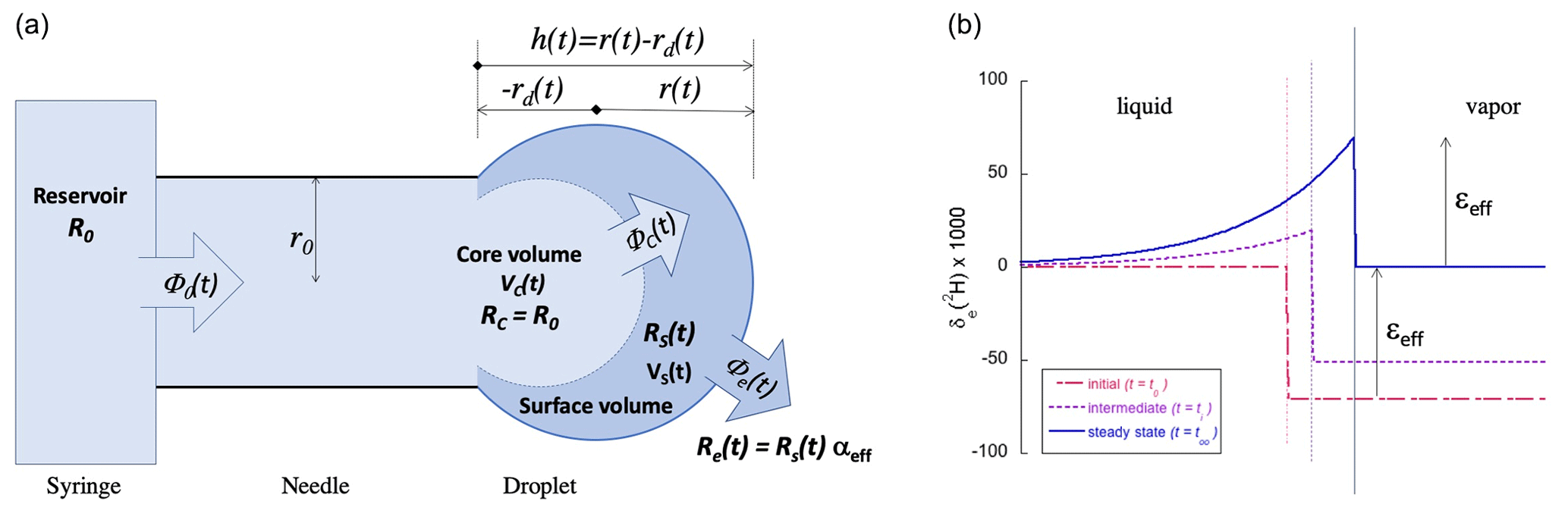
Figure 1 (a) Schematic representation of the ideal spherical droplet formed at the end of the syringe needle tip, illustrating the different reservoirs with volumes V, water fluxes Φ, and isotope ratios R involved in the model. As $r^{\mathrm{2}}=r_{\mathrm{0}}^{\mathrm{2}}+r_{\mathrm{d}}^{\mathrm{2}}$ and $r_{\mathrm{d}}=r-h$, it follows that $r=\left(r_{\mathrm{0}}^{\mathrm{2}}+h^{\mathrm{2}}\right)/\left(\mathrm{2}h\right)$. (b) The isotope ratio profile over the liquid to vapor boundary (left to right, with the thin vertical lines representing the growing water surface) at three instants in time if the water flux Φ₀ from the syringe (with δ₀=0) follows a step function with Φ₀(t)=0 for t<t₀ and with ${\mathrm{\Phi }}_{\mathrm{0}}\left(t\right)=F>\mathrm{0}$ for t>t₀. The isotope fractionation is taken to be ${\mathit{ϵ}}_{\mathrm{eff}}\approx -\mathrm{71}$ ‰ for δ²H. While the droplet is growing, δ_e<δ₀. Eventually, at t=t_∞, the incoming water flux Φ₀ equals the evaporated water flux Φ_e and δ_e=δ₀.

For completeness, it is assumed that only a fraction f of the droplet volume (a boundary layer) becomes enriched. It will later be shown that the best model results are obtained by assuming that the entire droplet becomes enriched (f=1, see Sect. 3.1) – an observation that is further supported by considerations involving the relative speeds of isotopic diffusion and the water flow (Sect. 4.1). Figure 1b shows the radial isotope concentration profile inside the droplet and the neighboring vapor following a step function in the flow rate from zero to some fixed value at t=t₀. The actual form of the profile is not important for the model and could just as well be approximated by a square profile. Thus, four different bodies of water can be distinguished:

1. The first is the syringe reservoir with a constant isotope ratio R₀ and an outgoing water flux equal to Φ₀(t) determined by the syringe pump speed.

2. The second is the core volume of the droplet with an isotope ratio R_c=R₀ and a time-dependent volume V_c(t). The water flux from the core to the surface layer of the droplet is given by Φ_c(t). Only in steady state is Φ_c=Φ₀.

3. The third is a fraction f ($\mathrm{0}<f\le \mathrm{1}$) of the total droplet volume V_d(t) that will become enriched in the heavy isotope, V_s(t), with isotope ratio R_s(t):

   $$\begin{array}{}\text{(1)}& V_{\mathrm{s}}\left(t\right)=f\cdot V_{\mathrm{d}}\left(t\right).\end{array}$$

4. The last is the evaporated water flux Φ_e(t), leaving the droplet with isotope ratio $R_{\mathrm{e}}\left(t\right)=R_{\mathrm{s}}\left(t\right)\cdot {\mathit{\alpha }}_{\mathrm{eff}}$. Here, the relevant isotope fractionation factor is that between the vapor- and liquid-phase water: ${\mathit{\alpha }}_{\mathrm{eff}}=\left(\mathrm{1}+{\mathit{ϵ}}_{\mathrm{eff}}\right)<\mathrm{1}$.

A last essential part of the model is the assumption that the evaporation flux is proportional to the exposed surface area of the droplet:

$$\begin{array}{}\text{(2)}& {\mathrm{\Phi }}_{\mathrm{e}}\left(t\right)=k_{\mathrm{e}}\cdot A_{\mathrm{s}}\left(t\right).\end{array}$$

Figure 1 gives a schematic representation of our model, indicating the relevant water volumes and inter-volume fluxes as well as the isotope ratios R of each volume. Solving the model ab initio is not difficult and will be shown to give a qualitatively and quantitatively satisfactory description of the dynamics under realistic conditions.

The free input parameters to the model are (a) the fraction f of the droplet that becomes enriched, (b) the effective liquid-to-vapor fractionation factor α_eff, and (c) the evaporation rate k_e. The initial estimates of these parameters were obtained from previous studies by Cappa et al. (2003) and Luz et al. (2009) for α_eff and from Walton (2004) and Sefiane et al. (2009) for k_e. The values of these parameters that provide the best fit to the experimental data are subsequently rationalized in Sect. 4.1, 4.3, and 4.4.

The first task is to model the evaporated total water flux Φ_e(t) as a function of a variable input water flux Φ₀(t), driven by variations in the syringe pump speed. For this, the mass balance equation for the noncompressible fluid is written out in discrete time with time step dt:

$$\begin{array}{}\text{(3)}& V_{\mathrm{d}}(t+\text{dt})=V_{\mathrm{d}}\left(t\right)+\left({\mathrm{\Phi }}_{\mathrm{0}}\left(t\right)-{\mathrm{\Phi }}_{\mathrm{e}}\left(t\right)\right)\cdot \text{dt}.\end{array}$$

The evaporation flux Φ_e(t) is a function of the droplet size through Eq. (2). For simplicity, the droplet at the tip of the needle is modeled as a partial sphere, a spherical cap. The surface area of the spherical-cap-shaped droplet is given by the following equation (see Fig. 1):

$$\begin{array}{}\text{(4)}& A_{\mathrm{s}}\equiv A_{\mathrm{cap}}=\mathrm{2}\mathit{\pi }rh=\mathit{\pi }\left(r_{\mathrm{0}}^{\mathrm{2}}+h^{\mathrm{2}}\right),\end{array}$$

where r is the radius of curvature of the cap, h is the cap height ($\mathrm{0}\le h\le \mathrm{2}r$), and 2r₀ is the inner diameter of the needle, all as defined in Fig. 1. The volume of the droplet is equally a function of h:

$$\begin{array}{}\text{(5)}& V_{\mathrm{d}}\equiv V_{\mathrm{cap}}={\displaystyle \frac{\mathit{\pi }}{\mathrm{6}}}h\left(\mathrm{3}{r}_{\mathrm{0}}^{\mathrm{2}}+h^{\mathrm{2}}\right).\end{array}$$

A_s(t) and, thus, Φ_e(t) can then be expressed in terms of V_d by inversion of Eq. (5), with h(V_d) being obtained as the only real root of the cubic equation, giving

$$\begin{array}{}\text{(6)}& h\left(V_{\mathrm{d}}\right)={\displaystyle \frac{{\mathit{\alpha }}^{\mathrm{2}}-\mathrm{12}u}{\mathit{\alpha }}},\end{array}$$

where

$$\begin{array}{}\text{(7)}& \mathit{\alpha }:=\sqrt[\mathrm{3}]{\mathrm{108}v+\mathrm{12}\sqrt{\mathrm{12}{u}^{\mathrm{3}}+\mathrm{81}{v}^{\mathrm{2}}}}\end{array}$$

and

$$\begin{array}{}\text{(8)}& u:=\mathrm{3}{r}_{\mathrm{0}}^{\mathrm{2}},v:={\displaystyle \frac{\mathrm{6}{V}_{\mathrm{d}}}{\mathit{\pi }}}.\end{array}$$

The above already permits the expression of both the droplet size (e.g., in terms of the droplet radius $r\left(t\right)=\left(r_{\mathrm{0}}^{\mathrm{2}}+h(t{)}^{\mathrm{2}}\right)/\left(\mathrm{2}h\left(t\right)\right)$) and the evaporative water flux Φ_e(t) as a function of V_d(t) as well as the subsequent calculation of both as function of the time-dependent input water flux Φ₀(t) by numerical integration of Eq. (3).

Going one step further, a second mass balance equation is included in the model to account for the rare isotopologues (in this case, either ²H¹⁶O¹H or ¹H¹⁸O¹H). First, the rare isotope fluxes (identified by ^*) are expressed in terms of the total fluxes and the isotope ratio of the reservoir in question. For the three relevant fluxes, this results in the following (see Fig. 1):

$$\begin{array}{}\text{(9)}& {\mathrm{\Phi }}_{\mathrm{0}}^{*}={\mathrm{\Phi }}_{\mathrm{0}}{\displaystyle \frac{R_{\mathrm{0}}}{\mathrm{1}+R_{\mathrm{0}}}}={\mathrm{\Phi }}_{\mathrm{0}}{\displaystyle \frac{R_{\mathrm{VSMOW}}\left(\mathrm{1}+{\mathit{\delta }}_{\mathrm{0}}\right)}{\mathrm{1}+R_{\mathrm{VSMOW}}\left(\mathrm{1}+{\mathit{\delta }}_{\mathrm{0}}\right)}};\end{array}$$

$$\begin{array}{}\text{(10)}& {\mathrm{\Phi }}_{\mathrm{c}}^{*}={\mathrm{\Phi }}_{\mathrm{c}}{\displaystyle \frac{R_{\mathrm{0}}}{\mathrm{1}+R_{\mathrm{0}}}}={\mathrm{\Phi }}_{\mathrm{c}}{\displaystyle \frac{R_{\mathrm{VSMOW}}\left(\mathrm{1}+{\mathit{\delta }}_{\mathrm{0}}\right)}{\mathrm{1}+R_{\mathrm{VSMOW}}\left(\mathrm{1}+{\mathit{\delta }}_{\mathrm{0}}\right)}};\end{array}$$

$$\begin{array}{}\text{(11)}& \begin{array}{rl}{\mathrm{\Phi }}_{\mathrm{e}}^{*}& ={\mathrm{\Phi }}_{\mathrm{e}}{\displaystyle \frac{R_{\mathrm{s}}{\mathit{\alpha }}_{\mathrm{eff}}}{\mathrm{1}+R_{\mathrm{s}}{\mathit{\alpha }}_{\mathrm{eff}}}}={\mathrm{\Phi }}_{\mathrm{e}}{\displaystyle \frac{R_{\mathrm{VSMOW}}\left(\mathrm{1}+{\mathit{\delta }}_{\mathrm{0}}\right){\mathit{\alpha }}_{\mathrm{eff}}}{\mathrm{1}+R_{\mathrm{VSMOW}}\left(\mathrm{1}+{\mathit{\delta }}_{\mathrm{0}}\right){\mathit{\alpha }}_{\mathrm{eff}}}}\\ & \approx {\mathrm{\Phi }}_{\mathrm{e}}{\displaystyle \frac{R_{\mathrm{VSMOW}}\left(\mathrm{1}+{\mathit{\delta }}_{\mathrm{0}}\right){\mathit{\alpha }}_{\mathrm{eff}}}{\mathrm{1}+R_{\mathrm{VSMOW}}\left(\mathrm{1}+{\mathit{\delta }}_{\mathrm{0}}\right)}}.\end{array}\end{array}$$

Recall that R_w is the ratio of the abundance of the rare to the most abundant water isotope in the reservoir w (w=0, c, s, e for the syringe and needle, the core of the droplet, the droplet surface layer, and the evaporated water, respectively). Thus, the factors (1+R_w) in Eqs. (9), (10), and (11) account for the conversion from the isotope abundance ratio to the isotope concentration. Finally, the fractionation factor between the (evaporated) vapor-phase water and the liquid α_eff≈1 (ϵ_eff≪1), making the approximation formed in Eq. (11) a very good one.

Equations similar to Eqs. (9), (10), and (11) hold for the different water reservoir volumes, allowing us to write the following for the volume of the isotopically enriched evaporating surface layer:

$$\begin{array}{}\text{(12)}& \begin{array}{rl}{V}_{\mathrm{s}}(t+\text{dt})& {\displaystyle \frac{R_{\mathrm{s}}(t+\text{dt})}{\mathrm{1}+R_{\mathrm{s}}(t+\text{dt})}}=V_{\mathrm{s}}\left(t\right){\displaystyle \frac{R_{\mathrm{s}}\left(t\right)}{\mathrm{1}+R_{\mathrm{s}}\left(t\right)}}\\ & +\left({\mathrm{\Phi }}_{\mathrm{c}}\left(t\right){\displaystyle \frac{R_{\mathrm{0}}}{\mathrm{1}+R_{\mathrm{0}}}}-{\mathrm{\Phi }}_{\mathrm{e}}^{*}\left(t\right)\right)\text{dt}.\end{array}\end{array}$$

Substituting

$$\begin{array}{}\text{(13)}& {\mathrm{\Phi }}_{\mathrm{c}}\left(t\right)={\mathrm{\Phi }}_{\mathrm{0}}\left(t\right)-{\displaystyle \frac{\mathrm{d}{V}_{\mathrm{c}}\left(t\right)}{\text{dt}}}={\mathrm{\Phi }}_{\mathrm{0}}\left(t\right)-{\displaystyle \frac{\mathrm{d}{V}_{\mathrm{d}}\left(t\right)-\mathrm{d}{V}_{\mathrm{s}}\left(t\right)}{\text{dt}}}\end{array}$$

and using the definition

$$\begin{array}{}\text{(14)}& \mathit{\psi }\left(t\right):={\displaystyle \frac{R_{\mathrm{s}}\left(t\right)}{\mathrm{1}+R_{\mathrm{s}}\left(t\right)}}\end{array}$$

then yields

$$\begin{array}{}\text{(15)}& \begin{array}{rl}& \mathit{\psi }(t+\text{dt}):=\\ & {\displaystyle \frac{\mathrm{1}}{V_{\mathrm{s}}(t+\text{dt})}}\mathit{\left\{}{V}_{\mathrm{s}}\right(t\left)\mathit{\psi }\right(t)+(\left(V_{\mathrm{s}}\right(t+\text{dt})-V_{\mathrm{s}}(t\left)\right)\\ & -\left(V_{\mathrm{d}}\right(t+\text{dt})-V_{\mathrm{d}}(t\left)\right)){\displaystyle \frac{R_{\mathrm{0}}}{\mathrm{1}+R_{\mathrm{0}}}}\\ & +\left({\mathrm{\Phi }}_{\mathrm{0}}\left(t\right){\displaystyle \frac{R_{\mathrm{0}}}{\mathrm{1}+R_{\mathrm{0}}}}-{\mathrm{\Phi }}_{\mathrm{e}}\left(t\right)\mathit{\psi }\left(t\right){\mathit{\alpha }}_{\mathrm{eff}}\right)\text{dt}\mathit{\}},\end{array}\end{array}$$

where the approximation for ${\mathrm{\Phi }}_{\mathrm{e}}^{*}\left(t\right)$ from Eq. (11) has been used.

The isotope ratio in the enriched fraction f of the droplet volume (using Eq. 1 and an appropriate value of f) can now be calculated by integration of Eq. (15) while evaluating Eq. (1) to Eq. (4) at each time step. The isotope ratio of the evaporated water is then obtained as

$$\begin{array}{}\text{(16)}& {\mathit{\delta }}_{\mathrm{e}}\left(t\right)={\mathit{\alpha }}_{\mathrm{eff}}\left(\mathrm{1}+{\mathit{\delta }}_{\mathrm{s}}\left(t\right)\right)-\mathrm{1},\end{array}$$

with

$$\begin{array}{}\text{(17)}& {\mathit{\delta }}_{\mathrm{s}}\left(t\right)={\displaystyle \frac{R_{\mathrm{s}}\left(t\right)}{R_{\mathrm{VSMOW}}}}-\mathrm{1}\end{array}$$

and

$$\begin{array}{}\text{(18)}& R_{\mathrm{s}}\left(t\right)={\displaystyle \frac{\mathit{\psi }\left(t\right)}{\mathrm{1}+\mathit{\psi }\left(t\right)}}.\end{array}$$

3 Results

The above model has been programmed in Mathcad (PTC Mathcad, 2020) and used to simulate data that were recorded with a high-precision, low-humidity water isotope spectrometer, named HiFI, described in Landsberg (2014) and Landsberg et al. (2014). As we are specifically interested in the dynamic behavior of the water vapor source that feeds the spectrometer, it is necessary to take the response time of the spectrometer into account. This response is typically described by a double or even triple exponential. At humidity levels of several thousand parts per million by volume (ppmv), the initial (fast) response time of the bare spectrometer was determined to be in the range of 1 to 2 s for both the water concentration and the isotope ratios, with a second, slower exponential response of the order of 15 s. However, in the configuration of this study and at the lower water concentrations of a few hundred parts per million by volume, the response time is significantly longer, especially for the δ²H isotope ratio. These response times were measured using the previously mentioned prototype humidity source (see Sect. 1), a predecessor of the isotopic humidity generator described in Leroy-Dos Santos et al. (2021), which was equipped with two independent syringe pumps, enabling rapid switching between two different water sources using a two-position, four-port valve (Vici Valco EUDA-4UWE) just before the spectrometer (Landsberg, 2014). The humidified air stream was sent either to the spectrometer or to a waste pump. The isotope response was determined by switching between two very different water standards, assuring a high signal-to-noise ratio of the measurements while keeping the concentration constant at about 600 ppmv. The standard waters used were working standards of the Groningen Center for Isotope Research (CIO), known as GS-48 (δ¹⁸O $=-\mathrm{6.3}$ ‰, δ²H $=-\mathrm{43}$ ‰) and BEW-2 (δ¹⁸O =795 ‰, δ²H =5983 ‰). It is noted that, despite careful storage, these absolute isotopic compositions can no longer be guaranteed with the precision specified by the CIO, as the standards had previously been used for other experiments. For all measurements shown here, the water isotope analyzer was calibrated with respect to the same water (GS-48) used for the evaporation measurements, resulting in relative isotope deviations (δ-values) equal to zero under steady-state conditions. Therefore, the absolute isotope ratios are not relevant. In any case, the drift of the standards was estimated to be less than 1 ‰ for δ²H and less than 0.2 ‰ for δ¹⁸O (due to possible Rayleigh distillation).

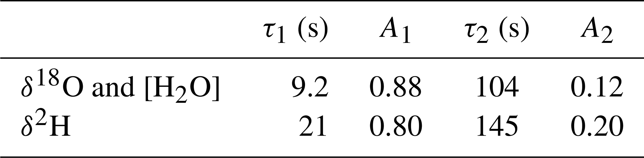
The instrument isotope response curves are shown in Fig. 2, and the double exponential fit parameters are summarized in Table 1. Whereas the total water vapor concentration and δ¹⁸O show practically the same time response, δ²H is about twice as slow, due to different time constants for the surface adsorption processes. Although at much higher humidity, Steen-Larsen et al. (2014) observed a qualitatively similar behavior. In the following sections, the time response of the spectrometer is taken into account, by convolution of the simulated response of the humidity generator with the calculated impulse response of the spectrometer that corresponds to the step response of Fig. 2, before comparison to the corresponding experimental data.

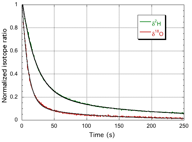
Figure 2 The normalized response curves of the spectrometer for switching between the GS-48 and BEW-2 isotope standards, both prepared as a mixture of ∼600 ppmv water vapor in dry air. The experimental data are fit with a double exponential, yielding 9.2 and 20.7 s for the fast decay times for δ¹⁸O (red curve) and δ²H (green curve), respectively. It is noted that the update frequency of the water isotope spectrometer is 2 Hz (Landsberg et al., 2014).

Table 1 Parameters of the double exponential fit to the measured instrument response for δ¹⁸O and δ²H. The water vapor concentration is observed to closely follow the δ¹⁸O behavior and was modeled with the δ¹⁸O parameters.

3.1 Humidity and isotope step responses

The model detailed in Sect. 2 was first used to simulate the dynamic behavior of the combination of the LHLG and the HiFI isotope analyzer, while the LHLG was programmed to generate small humidity steps of about 200 ppmv around an absolute value of roughly 400 ppmv. The simulated water vapor concentration response was fit to the experimental data by adjusting the evaporation rate k_e, the only free parameter in this case (see the top panel of Fig. 3). The rationale for the values of k_e determined in this study will be discussed in Sect. 4.4. Having fixed the evaporation rate at an optimal value of k_e=3 µm s⁻¹, the next step is to confirm that the isotope responses are modeled correctly, considering that both the δ²H and δ¹⁸O simulated responses also depend on the fraction f of the droplet volume that becomes enriched, as well as the effective liquid-to-vapor fractionation factor α_eff. As it can be expected that the entire droplet becomes enriched in the heavy isotopologues, the logical starting point is the assumption that f=1. As we will see shortly, this choice is validated by the experimental observations. It will subsequently be rationalized by theoretical considerations in Sect. 4.1.

Figure 3 Experimental data (gray curves) and model simulations of the humidity (blue traces; top) and isotope response curves (green for δ²H and red for δ¹⁸O; bottom) for three different values of the evaporation rate k_e. The best fit is obtained for k_e≈3 µm s⁻¹, whereas a higher (lower) value results in a simulated dynamic response that is too fast (slow) compared with the measured response.

Regarding the fractionation factors, at the very low relative humidity of the experiment (h≈0.01), the effective fractionation factors α_eff can be written as the product of a diffusion fractionation factor α_diff and an equilibrium fractionation factor α_eq (Cappa et al., 2003). Moreover, the diffusion fractionation factor can be related to the ratio of the molecular diffusivities (Stewart, 1975), such that one may write

$$\begin{array}{}\text{(19)}& {}^x{\mathit{\alpha }}_{\mathrm{eff}}{=}^x{\mathit{\alpha }}_{\mathrm{eq}}{\left({\displaystyle \frac{D\left(x\right)}{D\left(a\right)}}\right)}^n.\end{array}$$

As before, the label x refers to the rare isotope or isotopologue (²H and ¹⁸O or ²H¹⁶O¹H and ${}^{\mathrm{1}}{\mathrm{H}}_{\mathrm{2}}^{\mathrm{18}}\mathrm{O}$), and a refers to the abundant isotope or isotopologue (¹H and ¹⁶O or ${}^{\mathrm{1}}{\mathrm{H}}_{\mathrm{2}}^{\mathrm{16}}\mathrm{O}$). Thus, the effective fractionation factors for ²H¹⁶O¹H and ${}^{\mathrm{1}}{\mathrm{H}}_{\mathrm{2}}^{\mathrm{18}}\mathrm{O}$ are not independent but are determined by the single parameter n. The exponent n in Eq. (19) equals unity in the case of laminar flow and equals zero in the case of fully turbulent flow. The equilibrium fractionation factors were accurately determined by Horita and Wesolowski (1994), and their values at 35 ^∘C – the temperature of the evaporation chamber – are used here. The diffusivities were determined by Cappa et al. (2003) and more recently by Luz et al. (2009). The more recent values are used here, but the difference is minimal for our purpose (Cappa et al., 2003, predict only slightly lower values of α_eff in the laminar limit of n=1). Table 2 gives the values of the effective liquid-to-vapor fractionation factors for three different values of the flow parameter n, and Fig. 4 shows the corresponding model simulations compared to experimental data. The δ¹⁸O simulation shows a larger effect of changing n than the δ²H simulation. In contrast, changing the values of f has the same relative effect on both simulations (not shown in Fig. 4). With n=0.43 and f=1, a good fit to both isotope response curves is obtained. Thus, one may also conclude that the data support the theoretical finding (Sect. 4.1) that f=1. A good observer will have noted the difference in magnitude and noise level of the δ²H and δ¹⁸O responses shown in Figs. 3 and 4. Both are easily explained by noting that the isotopic fractionation is larger for ²H than for ¹⁸O, while the signal-to-noise ratio of the deuterium feature detected by the infrared spectrometer is concurrently significantly lower than that of ${}^{\mathrm{1}}{\mathrm{H}}_{\mathrm{2}}^{\mathrm{16}}\mathrm{O}$, which, in turn, is directly related to the lower abundance of ²H¹⁶O¹H with respect to ¹H¹⁸O¹H in the natural water sample.

Table 2 Effective fractionation factors as a function of the flow parameter n. For n=0, the fractionation factors are equal to the equilibrium values at 35 ^∘C, as determined by Horita and Wesolowski (1994).

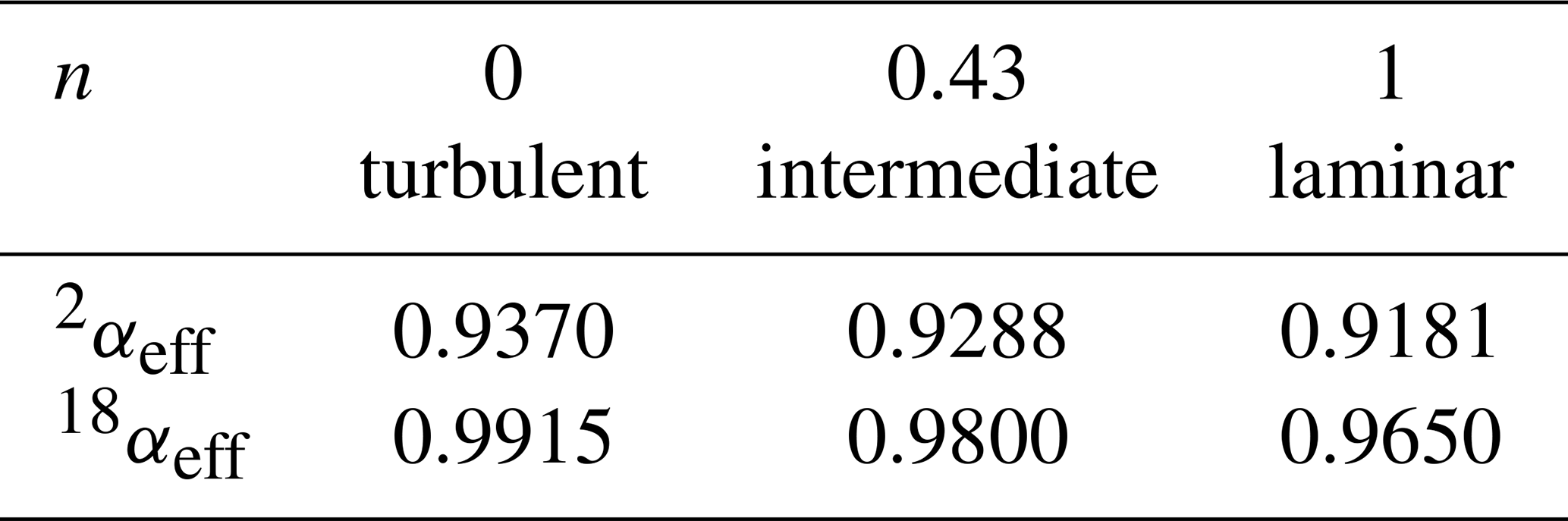
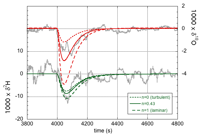
Figure 4 Experimental data (gray curves) and model simulations of the isotope response curves (green for δ²H and red for δ¹⁸O) for three different values of the flow parameter n. n=0 (dotted lines) corresponds to the turbulent flow limit, whereas n=1 (dashed lines) corresponds to the limit of laminar flow. For n=0.43 (solid lines), a good fit is obtained for both isotopes.

3.2 Dynamic response under nonideal conditions

The LHLG prototype was modified immediately following the experiments presented in the previous section. Notably, it was deemed that the bore of the aluminum injector chamber that accepts the syringe's needle was too narrow. With an internal diameter of only 2 mm, careful guidance of the needle and precise positioning of the syringe was needed to avoid occasional contact of the droplet with the chamber wall. This also limited the maximum droplet size and, therewith, the volume mixing ratio (humidity level) that could be attained to roughly 1000 ppmv. The injection chamber was therefore replaced by a stainless-steel sample cylinder with a volume of 75 mL and a Sulfinert hydrophobic coating (Restek 304L-HDF4-75). Because the flow velocity is now significantly lower, the coating serves to minimize the memory effect due to surface adsorption of water molecules. In addition, a section of polytetrafluoroethylene (PTFE) tubing was added between the syringe (Hamilton 84853) and the removable needle to make the alignment more easily manageable. This initially gave rise to unexpected results that were attributed to the appearance of small air bubbles in the water injection line. These problems were later resolved by reengineering the LHLG as described in Leroy-Dos Santos et al. (2021). These “useless” results that otherwise might have been discarded are reported here anyway because they nicely demonstrate the ability of the model to simulate the behavior of this nonideal instrument; thus, they validate the model under a different operating regime.

During similar experiments to those reported in Sect. 3.1, recording the response of the LHLG following small steps in the flow of injected water, relatively large sinusoidal oscillations were observed with a period that matched the revolution speed of the lead screw of the precision pump. It is proposed that these oscillations become prominently visible when small imperfections in the lead screw combine with small air bubbles present in the water injection line, possibly amplified by viscous resistance of the liquid inside the water line and needle. Whatever the precise underlying mechanics, a sinusoidal variation of the water flow was modeled with a period equal to one revolution of the screw drive. The amplitude and phase of the (possibly amplified) lead screw imperfection was chosen to yield a simulation that best matched the observed amplitude of the oscillations. The only other parameter that needed adjustment was the evaporation rate. A value of k_e=1 µm s⁻¹ was found to produce a simulation that best matched the water vapor concentration response when the pump was switched between different water flow rates, as seen in Fig. 5a. The lower evaporation is due to the lower flow velocity of the air around the droplet (see Sect. 4.4).

Figure 5 Humidity (a) and isotope responses (b) of the modified LHLG subject to stepwise changes in the water flow rate. The best fit (blue for the humidity response, green for δ²H, and red for δ¹⁸O) to the experimental data (gray curves) is obtained for an evaporation rate of k_e=1 µm s⁻¹. The overshoot in the first measured downward humidity transition and the corresponding inverted isotope response are most likely due to an air bubble in the water line.

The corresponding response of the isotope ratios is shown in Fig. 5b. It may be clear that the correspondence between simulation and experiment is (already) satisfactory, considering that no further parameter adjustments were made. The simulation will be further refined in Sect. 4.3.

4 Discussion

4.1 Droplet isotopic enrichment

Here, support is provided for the observation of an enrichment in the heavy isotopologues of the entire droplet and not just in a surface layer of limited thickness. Referring to Fig. 4 (for which n=0.43, i.e., ¹⁸α_eff=0.98, and f=1), in principle the same amplitude of the modeled response can be obtained by assuming fully laminar flow (n=1) and assuming that a much smaller fraction of the droplet becomes enriched in the heavy isotopes. However, this gives a less satisfactory fit to the data, as shown in Fig. 6. Notably, the response simulated with n=1 (i.e., ¹⁸α_eff=0.9650) and f=0.5 reached the same maximum amplitude, but it is clearly narrower than the experimental curve. Importantly, this is also not what is predicted based on the speed of isotopic diffusion in the droplet.

Figure 6 Experimental data and model simulations of the ¹⁸O response curves for two different values of α_eff and two different values of f.

To see that f is equal to unity in the present experiment, I consider that the enrichment occurring at the surface of the droplet will diffuse inwards, resulting in an isotope gradient inside the droplet with a characteristic diffusion length given by Bird et al. (2006):

$$\begin{array}{}\text{(20)}& L=\mathrm{2}\sqrt{D\cdot t},\end{array}$$

where D is the diffusion coefficient and t is time. Differentiation of Eq. (20) yields the velocity of the diffusion front:

$$\begin{array}{}\text{(21)}& v_{\mathrm{diff}}=\sqrt{{\displaystyle \frac{D}{t}}}.\end{array}$$

The diffusion coefficients of HDO and H¹⁸OH in water measured by Horita and Cole have been reported to be $\mathrm{2.34}\times {\mathrm{10}}^{-\mathrm{9}}$ and $\mathrm{2.66}\times {\mathrm{10}}^{-\mathrm{9}}$ m² s⁻¹, respectively (Horita and Cole, 2004). This shows that diffusion over lengths comparable to the size of a typical droplet (0.1 mm) takes place on a timescale of the order of 1 s. Thus, it is likely that the entire droplet becomes isotopically enriched, rather than just a surface layer: f=1.

4.2 Back diffusion

The question arises as to whether the diffusion is strong enough to allow the isotopic enrichment to propagate all the way to the syringe reservoir. To answer this question, the diffusion velocity of Eq. (21) is compared to the flow velocity inside the syringe needle:

$$\begin{array}{}\text{(22)}& v_{\mathrm{flow}}={\displaystyle \frac{{\mathrm{\Phi }}_{\mathrm{0}}}{A_{\mathrm{0}}}},\end{array}$$

where Φ₀ is the water flux through the syringe needle, and A₀ is the needle's internal cross-sectional area. After a characteristic time t_e, the diffusion velocity will have become smaller than the flow velocity, at which point in time the diffusion front does not further penetrate into the needle. This characteristic time equals

$$\begin{array}{}\text{(23)}& t_{\mathrm{e}}=D{\left({\displaystyle \frac{A_{\mathrm{0}}}{{\mathrm{\Phi }}_{\mathrm{0}}}}\right)}^{\mathrm{2}}.\end{array}$$

With typical values for the prototype instrument (an inner diameter of 464 µm for the 26-gauge needle and a low water flux of about 100 nL min⁻¹), the flow velocity inside the needle is about 0.6 mm min⁻¹, such that t_e≈25 s. Equation (20) then shows that the enrichment propagates about 0.5 mm into the 51 mm long needle. Moreover, at the given flow rate, it takes about 600 s to arrive at the typical droplet size of 10 µL. In this case, the isotopic diffusion into the needle stops before steady state is reached. Even at the lowest water flow rates of about 0.1 nL min⁻¹, the diffusion can be stopped well within the length of the needle (if necessary by reducing the needle inner diameter). Thus, it is unlikely that the isotopic composition of the syringe reservoir would change due to back diffusion of heavier isotopologues. This was also confirmed experimentally by bringing the same liquid standard material into the vapor phase with both the LHLG and a commercial humidity generator (Picarro SDM) at time intervals of 1 month and not observing any difference between the measurements (within a measurement precision of 0.2 ‰ and 1 ‰ for δ¹⁸O and δ²H, respectively) (Leroy-Dos Santos et al., 2021).

4.3 Fractionation factors

The effect of the precise values of the ²H¹⁶O¹H- and ${\mathrm{H}}_{\mathrm{2}}^{\mathrm{18}}\mathrm{O}$-isotopologue effective fractionation factors on the simulations has already been discussed to some extent in Sect. 3.1, where it was found that the best match with experiment is obtained by assuming fractionation factors that correspond to an intermediate case between laminar and turbulent flow (characterized by n=0.43). This can be rationalized by estimating the Reynolds number for the flow around the water droplet, $\mathit{Re}=\mathit{\rho }vL/\mathit{\mu }$. In the previous formula, ρ≈1.25 kg m⁻³ is the density of the air flowing around the needle and droplet; v=1.6 m s⁻¹ is the velocity of the air around the droplet inside the narrow-bore chamber (inner diameter 2 mm), given the air flow of 300 mL min⁻¹ (standard temperature and pressure); L≈0.5 mm is the diameter of the droplet; and μ=18.3 µPa s⁻¹ is the dynamic viscosity of air at 35 ^∘C. With these values, Re≈60. This contrasts with a value of v≈0.007 m s⁻¹ and Re≈0.2 for the case of the approximately 30 mm internal diameter steel cylinder used in the modified instrument. Therefore, the latter case should be much closer to the limit of fully laminar flow. The simulations in Fig. 5 were consequently repeated – but now with the fractionation factors for n=1 (see Table 2). The new simulations are shown in Fig. 7.

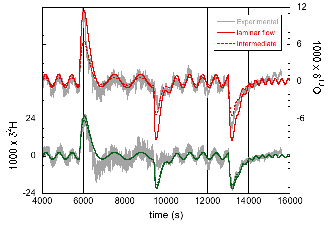
Figure 7 The isotope response of the modified LHLG subject to stepwise changes in the water flow rate. Improved simulations (compared with those in Fig. 5) are obtained with k_e=1 µm s⁻¹ and effective fractionation factors for the limiting case of fully laminar flow.

Whereas the differences for ²H are minor, the effect of the larger ¹⁸O fractionation (i.e., the smaller liquid-to-vapor fractionation factor, which is smaller than unity) in the laminar flow regime is clearly visible, and it arguably provides a slightly better fit to the data, primarily during the water vapor concentration changes, as can be seen in Fig. 7. It should be noted, however, that in the regions of oscillatory behavior in between the concentration steps, the fit could also have been nudged by adjusting the amplitude of the lead screw modulation. Still, the results of Sect. 3.2 are just as well (or better) described (than shown in Fig. 5) by assuming fully laminar flow.

4.4 Evaporation rate

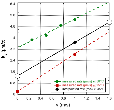
The two experiments discussed here in Sect. 3.1 and 3.2 required rather different evaporation rates to simulate the data with our model, k_e≈3 and 1 µm s⁻¹, respectively. The difference is clearly related to the different Reynolds numbers or, more directly, the different dry-air flow velocities of 1.6 and 0.007 m s⁻¹. In fact, the values are in reasonable agreement with the results reported by Walton (2004). Although his measurements were recorded at only a small number of air temperatures and flow velocities, values applicable to our situation can be estimated by linear extrapolation of the observed rates as a function of flow velocity, and fitting a (weakly) quadratic dependence on the temperature to the data collected at a fixed flow velocity of 1 m s⁻¹. In Fig. 8, selected data from Walton (2004) are presented along with the estimated values for our case. Thus, one predicts a rate of 5.2 µm s⁻¹ at a flow velocity v=1.6 m s⁻¹ and a rate of 1.3 µm s⁻¹ at a flow velocity v=0 m s⁻¹, which are higher than the experimental values found here. So far, it has been assumed that the droplet is at the same temperature as the evaporation chamber, but it cannot be excluded that the actual droplet temperature is lower, especially in the high-velocity case. However, the study by Sefiane et al. (2009) measured an evaporation rate at 22 ^∘C and 1 bar, corresponding to ∼4 µm s⁻¹, which is very close to the value extrapolated from the data of Walton (2004) at 25 ^∘C. It is noted that the observation of a slightly lower evaporation rate than that found by Walton (2004) or Sefiane et al. (2009) is in agreement with the experimental sessile droplet, as it sits on the beveled tip of the syringe needle (Landsberg, 2014; Leroy-Dos Santos et al., 2021), having a somewhat smaller surface-to-volume ratio than the one that is modeled. It should also be mentioned that it is unlikely that the difference with the observations by Walton (2004) or Sefiane et al. (2009) are due to an underestimation of the spectrometer humidity response time, as it is difficult to imagine a response time of the water vapor concentration that is slower than that of the isotope ratios.

Figure 8 Evaporation rate measurements made by Walton (2004) as a function of flow velocity at 25 ^∘C (red solid squares) and at 50 ^∘C (green solid circles) as well as one interpolated point at 35 ^∘C (black solid diamond), leading to the extrapolated estimates for our experiment (open circles).

5 Conclusions

It has been shown that the dynamic behavior of a humidity generator based on droplet evaporation can be accurately modeled. Confrontation with experimental data of the water vapor concentration and two isotopic ratios as a function of the injected water flow enables the determination of physically realistic values of the droplet evaporation rate and the liquid-to-vapor isotope fractionation factors. However, the signal-to-noise ratio of the water isotope analyzer at the very low humidity levels investigated is not quite sufficient to make very precise determinations of the fractionation factors. However, recent developments in ultraprecise and ultrasensitive isotope measurements (e.g., Stoltmann, 2017; Kassi et al., 2018) will enable one to deliver more precise values by at least an order of magnitude. What may appear as a bit of a quixotic study of evaporating water droplets may, thus, in fact permit the measurement of not only the evaporation rate but also the effective fractionation factors and therewith also isotopologue-dependent diffusivity ratios, in the evaporation of small sessile droplets. Apart from this potentially new application, it is highly satisfactory to be able to accurately simulate the dynamic behavior of the LHLG with few free parameters and under rather different operating conditions.