the Creative Commons Attribution 4.0 License.
the Creative Commons Attribution 4.0 License.
 | 28 Jun 2021
Sensitivity of Aeolus HLOS winds to temperature and pressure specification in the L2B processor
Matic Šavli
Christophe Payan
Jean-François Mahfouf
The retrieval of wind from the first Doppler wind lidar of European Space Agency (ESA) launched in space in August 2018 is based on a series of corrections necessary to provide observations of a quality useful for numerical weather prediction (NWP). In this paper we examine the properties of the Rayleigh–Brillouin correction necessary for the retrieval of horizontal line-of-sight wind (HLOS) from a Fabry–Pérot interferometer. This correction is taking into account the atmospheric stratification, namely temperature and pressure information that are provided by a NWP model as suggested prior to launch. The main goal of the study is to evaluate the impact of errors in simulated atmospheric temperature and pressure information on the HLOS sensitivity by comparing the Integrated Forecast System (IFS) and Action de Recherche Petite Echelle Grande Echelle (ARPEGE) global model temperature and pressure short-term forecasts collocated with the Aeolus orbit. These errors are currently not taken into account in the computation of the HLOS error estimate since its contribution is believed to be small. This study largely confirms this statement to be a valid assumption, although it also shows that model errors could locally (i.e. jet-stream regions, below 700 hPa over both earth poles and in stratosphere) be significant. For future Aeolus follow-on missions this study suggests considering realistic estimations of errors in the HLOS retrieval algorithms, since this will lead to an improved estimation of the Rayleigh–Brillouin sensitivity uncertainty contributing to the HLOS error estimate and better exploitation of space lidar winds in NWP systems.
- Article
(5636 KB) - Full-text XML
- BibTeX
- EndNote


The ESA's Aeolus wind satellite was launched on 22 August 2018. Aeolus is one of the Earth Explorer missions proposed by ESA as a demonstration paving the way towards measuring wind from space globally (Stoffelen et al., 2005). In this view the continuous effort to better understand and to improve the wind retrieval has been undertaken by ESA, Aeolus Data Innovation and Science Cluster (DISC), and Aeolus CAL/VAL teams since launch. In particular, an increasing effort is undertaken to better understand the various sources of observation errors. Such is a systematic error arising due to a so-called dark current signal anomalies of single accumulation charge-coupled device (ACCD) pixels (i.e. “hot pixel”) (Weiler et al., 2020) or a significant source of wind systematic error which has been found to be correlated with the temperature gradients across the Atmospheric Laser Doppler Instrument (ALADIN) primary mirror M1 of the telescope (Rennie and Isaksen, 2020). Despite the relatively large observation errors of the Aeolus wind observations compared to radiosondes or airborne lidar wind observations (e.g. Witschas et al., 2020; Martin et al., 2021), a list of OSEs (observation system experiments) provided by various global and regional models showed a significant impact on the numerical weather prediction (NWP; Aeolus CAL/VAL workshop: https://nikal.eventsair.com/QuickEventWebsitePortal/2nd-aeolus-post-launch-calval-and-science-workshop/aeolus, last access: 17 May 2021) such as was suggested by several pre-launch studies (e.g. Žagar, 2004; Tan and Andersson, 2005; Weissmann and Cardinali, 2006; Stoffelen et al., 2006; Tan et al., 2007; Marseille et al., 2007, 2008; Weissmann et al., 2012; Horanyi et al., 2015; Šavli et al., 2018). This led several weather centres1 to already start with the operational assimilation of the line-of-sight wind observations.
The main product of the Level-2B processor (L2Bp) is the horizontal line-of-sight (HLOS) wind, which is inferred by the Doppler shift of the backscattered light measured from a small volume in the atmosphere. The backscatter spectrum is sensed by two unique interferometers; the Fabry–Pérot (FP) which is used to measure Doppler shift mainly from moving molecules (Rayleigh channel) and the Fizeau which is used to measure Doppler shift mainly from aerosols and small hydrometeors (Mie channel) (e.g. Reitebuch, 2012). The Doppler shift measured from moving molecules is well described by the so-called Rayleigh–Brillouin spectrum which deviates from the ideal Gaussian spectrum. Two Brillouin peaks are introduced on each side of the Gaussian spectrum shifted in frequency by acoustic waves, as a consequence of the increased density of molecules (i.e. through collisions) lower in the atmosphere (Gu and Ubachs, 2014). The information on temperature and pressure, needed for properly modelling such Rayleigh–Brillouin spectrum characteristics, which should be collocated with the Aeolus measurements, is, however, not provided by Aeolus, nor is it available from the current Global Observation System (GOS). Therefore, the suggestion of Dabas et al. (2008) was to infer this information from a NWP which, on the other hand, contains errors which typically consist of model and representativeness errors and also errors from initial conditions.
The mean temperature forecast error is a well-monitored quantity; for example, it is monitored by the WMO Lead Centre for Deterministic Forecast Verification (WMO-LCDNV, https://apps.ecmwf.int/wmolcdnv/, last access: 17 May 2021). The RMSE of the temperature forecast from various operational global models is found typically to be less than 2 K for a 24 h forecast range in the extratropics. This error is smaller in the tropics, being slightly above 1 K. The majority of the distribution of a global model temperature remains below 3 K even for longer forecast ranges. Estimations provided by Dabas et al. (2008) suggest that in a standard atmosphere the temperature sensitivity of HLOS retrieval brings a relative HLOS error of about 0.2 % for 1 K error in temperature, which is well below the 0.7 % relative error specified as an ESA requirement (ESA, 2016). On the other hand, HLOS sensitivity to pressure suggests providing about an order of magnitude smaller impact with a typical model pressure error of few hectopascals. Compared to the current HLOS observation errors which are of the order of about 4 m s−1 (e.g. Martin et al., 2021), it appears to be a rather small overall contribution. However, it is necessary to take into account the fact that NWP forecast error varies spatially and temporally due to weather regimes present on various spatial and temporal scales that are not always well described but are also due to errors in initial conditions. Overall, for optimal Rayleigh–Brillouin correction in L2Bp the most accurate source of temperature and pressure information should be used.
The main goal of this paper is to explore the impact of the uncertainty in model forecast of temperature and pressure fields for the retrieval of Rayleigh HLOS winds. It is assumed that some properties of this sensitivity can be estimated by using two different model forecasts. Since the truth is not known it is not possible to estimate it adequately at each point in space and time. In particular, the two models chosen for this study share some similarities from the perspective of their design, data assimilation system and associated observation system leading to somewhat correlated forecast errors. This has an effect of leading to an overall underestimation of the true uncertainty in modelled temperature and pressure fields when forecasts are compared. Taking this into account, in this study we analyse the spatially and temporally averaged differences in model forecast temperature and pressure fields and the subsequent sensitivity of HLOS retrieval.
A brief introduction of the Rayleigh–Brillouin correction algorithm is first given in Sect. 2. Then the methodology of the sensitivity study is described in more detail in Sect. 3. Here the production of the auxiliary meteorological data input at Météo-France is described, exploiting the local installation of L2Bp. Several statistical validation metrics are presented as well. Results of the sensitivity study are presented in Sect. 4 followed by conclusions in Sect. 5.
The thorough description of L2Bp algorithm is beyond the scope of this paper, and the reader is invited to consult the existing literature (e.g. Tan et al., 2008; Stoffelen et al., 2005) and the L2Bp official documentation (Rennie et al., 2020). A brief overview of the Rayleigh HLOS retrieval from FP interferometer is, however, given to introduce the necessary methodology. The temperature and pressure information is used in a so-called Rayleigh–Brillouin correction algorithm. The information of the spectrometer counts is first used to compute a so-called Rayleigh response (RR), a quantity that is linearly related to the Doppler shift and hence to the HLOS wind, through a so-called response curve (Dabas et al., 2008). A Doppler shift νd is inferred from a calibration look-up table , which specifies the relation between a range of temperatures T, pressures p, RR and Doppler shift values. This table is provided using the information of backscatter spectrum computed by the Tenti S6 model (Tenti et al., 1974) and the interferometer transmission curves. In particular, for each Aeolus observation the Doppler shift is computed by a Taylor expansion as specified by Eq. (1).
where subscript 0 refers to the nearest values of measured RR and collocated T and p available from the look-up table. Three derivatives are estimated using a finite difference method, as well as from the look-up table.
An additional correction factor is taken into account as the signal from the FP interferometer is contaminated by the Mie signal. The relative contribution of the Mie signal is described by scattering ratio , where βaer and βmol are the particular and molecular backscatter ratio of the sensed volume of atmosphere. A tunable scattering ratio threshold parameter (ρt) is defined in the L2Bp (De Kloe et al., 2020) which further classifies in to a so-called “clear” and “cloudy” wind observations, thus Rayleigh clear for which scattering ratio is smaller than ρt and Rayleigh cloudy for larger values of scattering ratio. The value of ρt has been carefully tuned since the start of the mission and did vary from values of 1.25 in version v3.00 up to 1.6 in version v3.20. This increase led to generally improved classification (e.g. Rennie and Isaksen, 2020). For any value of scattering ratio larger than 1, an additional correction is applied on top of as specified in the following equation:
Taking into account the relation between line-of-sight wind LOS and Doppler shift, and λ0 the lidar base wavelength, the sensitivity parameters are provided, where X is T, p, RR or ρ. These are primarily used to estimate the Rayleigh HLOS wind observation instrumental error internally in the L2Bp, i.e. by assuming a typical uncertainty in temperature and pressure as well as for the scattering ratio. In addition, these sensitivities along with reference values of Tref, pref and ρref (T, p and ρ used in Eqs. 1–2) are provided as an output of the L2Bp which can be used for any additional correction of HLOS without the need for running L2Bp, considering the following equation:
where for X, and Xref is one of HLOS (HLOSref is the output of the L2Bp), T, p or ρ. Only linear terms are taken into account. Thus the correction is expected to be valid for small differences in T, p and ρ. Several additional correction schemes are applied in L2Bp (Rennie et al., 2020). However, these are not relevant for the present study.
Data needed for the above-mentioned correction are provided to L2Bp as a series of auxiliary files (Rennie et al., 2020) by the Aeolus Payload Data Ground Segment (PDGS). Three required data inputs have to be specified. The first is the Aeolus Level-1B wind vector mode product, which is the main input providing the information from the FP and Fizeau interferometers (e.g. spectrometer counts), geolocation information, calibration information and error estimates for several variables. This file is an output of the Level-1B processor. The second one is the auxiliary meteorological data input (further denoted AUX_MET), which provides the necessary information on atmospheric temperature and pressure as described previously. The operational AUX_MET data are produced in near-real time by the Level-2 Meteorological Processing Facility (L2/Met PF), which is a part of PDGS and is hosted by the European Centre for Medium-Range Weather Forecasts (ECMWF). The third one is the auxiliary input file, which provides information of the calibration look-up table and additional data used in the Rayleigh–Brillouin correction algorithm. Several optional additional input data provide information on the Aeolus-predicted orbit ground track geolocation, climatology of lidar ratio and lidar signal calibration constants. Finally, the additional necessary input file (further denoted AUX_PAR) provides the settings and parameters to control the L2Bp processing.
To validate the sensitivity of HLOS retrievals due to the Rayleigh–Brillouin scattering dependency on atmospheric temperature and pressure in operational L2Bp, we consider the Action de Recherche Petite Echelle Grande Echelle (ARPEGE) global NWP model (Courtier et al., 1991) to provide an independent realization of atmospheric temperature and pressure. This model will be used to provide the associated AUX_MET input files which are first assessed in a statistical inter-comparison with the default (i.e. operational) AUX_MET temperature and pressure of the ECMWF IFS model. Based on this comparison and on the sensitivity parameters ∂THLOS and ∂pHLOS, the characteristics of the HLOS uncertainty due to temperature and pressure differences are discussed. The ability of running L2Bp using ARPEGE-derived AUX_MET allows the additional evaluation of the value of the correction specified by Eq. (3) and the Mie-contamination contribution. The validation is undertaken for the Rayleigh-clear HLOS observations only, as equivalent sensitivity to temperature and pressure is expected for the Rayleigh-cloud HLOS observations.
3.1 Production of Level-2B auxiliary meteorological input at Météo-France
The AUX_MET auxiliary file provides profiles of several meteorological variables such as temperature, pressure, specific and relative humidities, and wind (as well as information on cloud cover and cloud liquid/ice water content) along the Aeolus orbit. The AUX_MET data are available for nadir (laser is pointing perpendicular towards the earth surface) and off-nadir (laser is tilted 35∘ off nadir). Currently, the L2/Met PF provides meteorological quantities as vertical profiles interpolated spatially and temporarily from a short-term IFS forecast having a validity from 6 to 30 h and produced twice per day. Representation of a slanted off-nadir data with a vertical profile has been found to be an acceptable simplification (e.g. Rennie et al., 2020). Indeed, the maximal difference in terms of geolocation between the model vertical profile and the Aeolus orbit is about 21 km at 30 km altitude, which is not significant given the effective resolution of the model that cannot resolve scales below around 100 km (e.g. Marseille and Stoffelen, 2017). This operational auxiliary meteorological file is denoted hereafter as AUX_METecmwf.
The production of auxiliary meteorological data at Météo-France (named AUX_METmf) is an offline procedure. In that respect the production of meteorological auxiliary files did not follow exactly the production at L2/Met PF, but it has been instead simplified allowing for minimal adaptation of existing operational ARPEGE routines at the time of the study.
A flowchart of the working processing chain is shown in Fig. 1. It is important to notice that a production of AUX_METmf is done every 6 h, which is consistent with the ARPEGE data assimilation system (Fig. 1b). For the purpose of explaining the behaviour of the chain, a production at 06:00 UTC is discussed next.
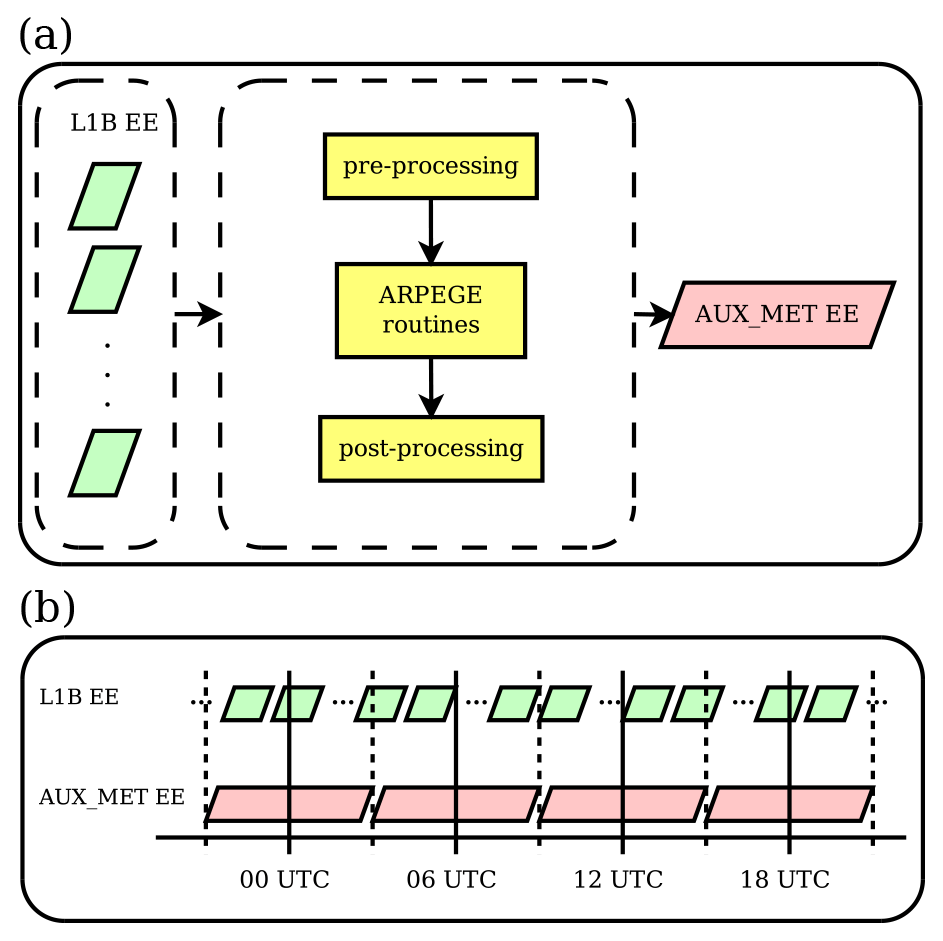
Figure 1Production of AUX_MET files at Météo-France. A detailed description is given in Sect. 3. The EE stands for Earth Explorer file format.
At Météo-France the L1B measurement geolocation is used to provide information on the Aeolus orbit needed for production of AUX_MET data. In particular, L1B output files store the geolocation for each measurement, which is ideally available every ∼3 km, being a baseline for the sampling distance of vertical profiles in the AUX_METmf. Similarly, as in AUX_METecmwf, AUX_METmf vertical profiles are provided both for the nadir and off-nadir. The geolocations are gathered from all available L1B data over the time period of 03:00 to 09:00 UTC (typically of about 5–6 L1B files). This is the main input dataset for the production of auxiliary meteorological files.
In the following stage, the extracted geolocation is first reformatted (pre-processing stage in Fig. 1a) in a way that is compatible with the ARPEGE data assimilation system through BUFR (Binary Universal Format for the Representation of meteorological data) files. Then, for each geolocation, model vertical profiles of several variables are extracted during the data assimilation window. These ARPEGE outputs in ODB (Observation Data Base) format are finally reformatted (in the post-processing stage in Fig. 1) into a single AUX_METmf file ready to be used in L2Bp. The chosen ARPEGE model configuration corresponds to the operational one (CY43T2). This spectral model has a stretched and tilted horizontal grid with the highest horizontal resolution over France (∼5 km) and the lowest (∼20 km) on the opposite pole (New Zealand). The model consists of 105 vertical levels defined in between 10 m and 0.1 hPa following a hybrid vertical coordinate. The model profiles are extracted from the ARPEGE model background trajectory in the so-called screening task. This is a part of the 4D-Var system where the model is run forward and compared to observations within 30 min time slots.
On top of various error sources affecting this sensitivity study (as discussed in Sect. 1), additional errors arise due to the specific configuration displayed in Fig. 1. In particular, AUX_METmf data represent a so-called first guess (a very short-term forecast of 3–9 h), whereas AUX_METecmwf data represent a longer-range forecast (6–30 h). Thus, the statistics of their differences are affected by differences in forecast lead times. Furthermore, since the two datasets are produced from two different operational data assimilation system implementations, their differences will further increase the complex interplay of various error sources and therefore the estimate of the uncertainty in temperature and pressure fields. These statements support the initial proposal to perform the analysis of the spatially and temporally averaged differences in model forecast temperature and pressure fields that will reduce some of these effects on the HLOS sensitivity.
In addition, one side effect of the configuration presented in Fig. 1 is that AUX_METmf files are not partly overlapping in time as is the case for the AUX_METecmwf files. Indeed, the validity of AUX_METmf files is exactly 6 h, which are produced four times per day, whereas AUX_METecmwf represents 6–30 h IFS forecast, the files which are produced twice per day. Therefore, when using AUX_METmf files in the L2Bp, a specific approach must be used in the case the L1B input file spans a time period in between two data assimilation windows of the ARPEGE system (i.e. two AUX_METmf files). In such a case the L2Bp must be run twice for each AUX_METmf file, and finally data from both L2B runs must be merged into one single L2B output.
3.2 Sensitivity study
From two distinct auxiliary meteorological data (AUX_METecmwf and AUX_METmf), covering the same Aeolus orbit section, it is possible to analyse differences induced by the two associated L2B HLOS retrievals. The necessary processing chain for performing such a study is displayed in Fig. 2. The part enclosed in the dashed lined box corresponds to the simplified operational L2B processing chain performed by the PDGS which essentially consists of running the L2Bp with all necessary input files and a configuration file. A similar chain of processes has been replicated locally at Météo-France, using the same L2Bp version, the same configuration file and the same input files, except for the AUX_METmf input file which is produced as described in Sect. 3.1. The statistical evaluation of the difference between the two HLOS wind products, to be explained in more details in Sect. 3.4, is shown in Fig. 2 by the two black arrows pointing towards the “statistical evaluation” box.
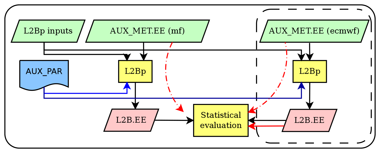
Figure 2Flowchart of L2B generation and sensitivity study set-ups. The detailed description is given in Sect. 3. The EE stands for Earth Explorer file format.
Another evaluation approach is used as is depicted by the three red arrows in Fig. 2. In this particular case the L2Bp is not used, but instead all the necessary information is directly extracted from the AUX_METecmwf and AUX_METmf files and the operational L2B product. As described in Sect. 2, given the small model differences in terms of temperature and pressure with respect to reference values (from IFS), it is possible to express the HLOS difference (Eq. 3) by a Taylor expansion. It is first assumed that the third term in Eq. (3) can be neglected, i.e. Δρ=0. Then, the computation of temperature and pressure differences (i.e. ΔT and Δp in Eq. 3) is done by comparing the two AUX_MET files. This has been possible by closely replicating the L2Bp algorithm that first interpolates temperature and pressure (the nearest profile from the AUX_MET) onto the HLOS measurement geolocation. Note that HLOS measurement is representative of ∼2.8 km, whereas HLOS observation represents the accumulation (i.e. average) of up to about 30 (for Rayleigh clear) measurements. The same averaging approach applies for temperature and pressure information representative of a particular HLOS observation. Finally, using the sensitivity values (∂THLOS and ∂pHLOS) available in the operational L2B output the HLOS difference has been computed.
3.3 Datasets and Level-2B processing
As Aeolus is an explorer mission the retrieval of HLOS winds from raw satellite data is continuously adapting and improving. The choice of selected dataset is therefore an important factor that should be taken into a consideration. For this particular study the dataset is part of the reprocessed one available for a period of July–December 2019 (i.e. baseline 2B10). This is an official reprocessing from PDGS and contains a number of improvements of several deficiencies closely examined by ESA and DISC. This is an improved treatment for removing spurious outliers induced by dark current signals (hot pixels) (Weiler et al., 2020). A dark current signal is measured when no laser pulse is emitted. Moreover, orbit variable systematic errors have been removed by an innovative method based on a linear relation of the satellite primary mirror temperature gradient and the model estimated HLOS systematic error (Rennie and Isaksen, 2020). In addition, since 1 August 2019 the Rayleigh–Brillouin correction has been affected by calibration update, having a direct impact on the properties studied in this paper. As a consequence, the dataset selected for this study is valid for the period of 1 August up to 31 December 2019. This dataset is used for the study, concerning the methodology of a second approach of the sensitivity validation (without using the L2Bp) as described in Sect. 3.2. On the other hand, data from the first Aeolus laser period (so-called FM-A period) are used for the experiment using L2Bp. In this case the dataset consists of 464 orbits from the period of 30 November 2018 to 13 January 2019. As this particular dataset has not yet been officially corrected, it can impact results presented afterwards. However, as will be discussed later this effect is expected to be small.
The L2Bp used here is of version 3.01. The configuration file of the processor (AUX_PAR) is of version 8 (used during baseline 2B02), which consists of a scattering ratio threshold of 1.5–1.6 for Rayleigh classification on clear and cloudy scenarios and a Rayleigh-clear accumulation length (i.e. the distance along the orbit for which the observation is representative) of 86.4 km.
3.4 Statistical evaluation
From L2B outputs only Rayleigh-clear information is used after applying a basic quality control. It consists of rejecting all observations identified as invalid (information available in the L2B output) or for which the L2B estimated observation error is larger than 10 m s−1 (similar to a range of values typically used in the quality control of several NWP centres assimilating Aeolus data). In addition, a quality check against the ARPEGE background is performed such that HLOS observations that differ significantly from ARPEGE-derived HLOS winds are discarded. This approach allows the study of the sensitivity properties only for data that would be considered for data assimilation in NWP models.
Main properties of ΔHLOS, ΔT and Δp are examined by using typical robust statistical metrics. Such are median (50th percentile of the distribution) and median absolute difference (mad) evaluated spatially and/or temporally, along with several other distribution percentiles. Median absolute difference is a robust measure of dispersion computed as a median of absolute difference of the original distribution with respect to its median (Wilks, 2011, chap. 3.1.2). These quantities are especially useful in case of outliers in the distribution. The so-called madn=1.48mad is used instead of mad since it agrees with the standard deviation when the sample distribution is Gaussian. The same approach is chosen to describe the statistical properties of the HLOS sensitivity terms, e.g. ∂THLOS.
4.1 Main characteristics of the HLOS sensitivity to temperature and pressure
Main properties of the sensitivity (i.e. ∂THLOS and ∂pHLOS) valid for the period from 1 August up to 31 December 2019 are shown in Fig. 3. Statistics as a function of HLOS wind velocity are displayed in Fig. 3a and b. These are computed by grouping available data in to 10 m s−1 HLOS wind velocity bins. In addition to the average sensitivity, measured by the median, the percentiles of 0.5 and 99.5 (as well as 25 and 75 for the sensitivity against pressure) are also computed to give an estimate of its variability for a particular range of HLOS wind velocities.
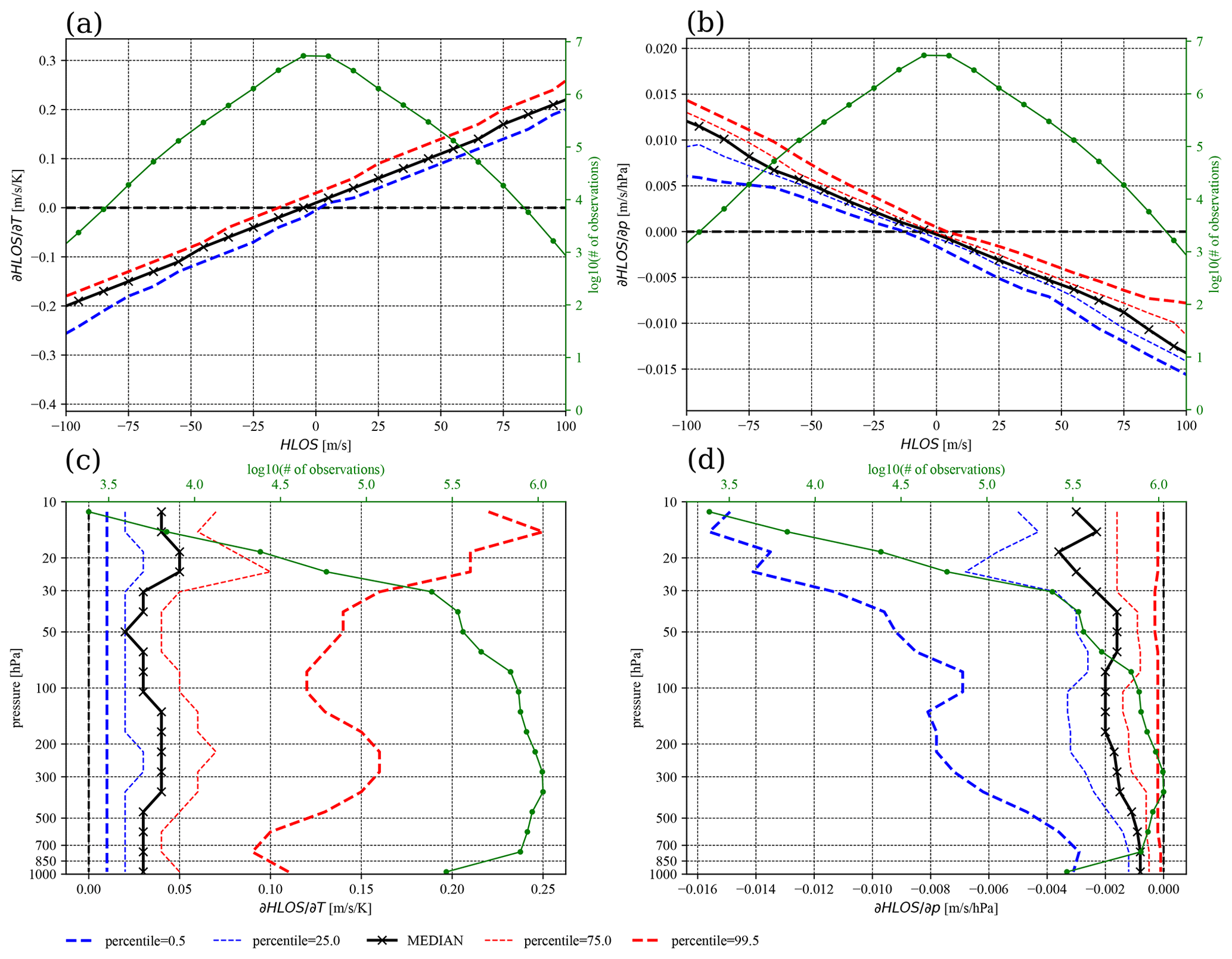
Figure 3The HLOS sensitivity (a, c) with respect to temperature (i.e. ∂THLOS) and (b, d) with respect to pressure (i.e. ∂pHLOS) over a 5-month period (1 August to 31 December 2019). (a, b) The sensitivity is shown as a function of HLOS wind velocity. The median and several percentiles are computed by gathering all available and valid data in HLOS bins of 10 m s−1. (c, d) The sensitivity is shown as a function of pressure taking into account only data with positive HLOS wind velocity. The amount of available data in a bin (solid green).
One property of the HLOS sensitivity to temperature is its approximate linear dependency with HLOS wind velocity. The slope of the median curve is ∼0.002 K−1, which is in good agreement with the value for the standard atmosphere given by Dabas et al. (2008). The variability shown by the two percentiles is mostly induced by the fact that inside each bin HLOS wind velocity varies by 10 m s−1 and is less effected by the fact that atmospheric conditions, i.e. temperature and pressure, vary significantly over the same range bin. The variability is rather consistent over the whole range of HLOS wind velocity.
As discussed in Sect. 2, by using properties of the sensitivity presented in Fig. 3a it is possible to approximately estimate the random error contribution since temperature information is not known exactly (i.e. based on Eq. 3). Typically, for a random error of 1 K in temperature the random error in HLOS would increase by only of about 0.2 m s−1 for a 100 m s−1 HLOS wind. However, for temperature differences of about 10 K, an increase of up to about 2 m s−1 in HLOS (for 100 m s−1 HLOS wind) is expected, i.e. a relative error of 2 %. As a consequence, outliers in the model temperature distribution are going to produce significant differences in HLOS retrievals.
Moreover, sensitivity varies in the vertical, as shown in Fig. 3c, as a function of pressure (i.e. altitude) but only for positive HLOS winds since it is symmetric for negative HLOS. The largest values are expected near the upper troposphere–lower stratosphere (UTLS), both of which are associated on average with globally stronger winds. Similarly, the sensitivity increases with altitude in the stratosphere due to the positive temperature gradient in this region.
On the other hand, the HLOS sensitivity to pressure is significantly less, given the small uncertainties in model pressure information. In particular, the sensitivity shown in Fig. 3b and d indicates a median value (over all positive HLOS) of about −0.002 , which is in the range of expected values (e.g. 0.003 for the standard atmosphere as shown by Dabas et al., 2008). The variability of the sensitivity (Fig. 3b) becomes stronger with larger absolute HLOS winds, which is induced by the effect of variable temperature and pressure conditions in a given HLOS bin. Therefore, a significant slope (especially for percentile 0.5) of the sensitivity with altitude is shown in Fig. 3d. With a 10 hPa (a typical root-mean-squared error of 24 h global model mean-sea-level forecast against analysis, https://apps.ecmwf.int/wmolcdnv/scores/mean/msl, last access: 17 May 2021) error in pressure, the random error in HLOS would increase by about 0.1 %, whereas a 100 hPa random error would increase the HLOS error by 1 %. The effect of the pressure sensitivity is thus expected to be at least 1 order of magnitude smaller compared to the temperature sensitivity when the NWP model pressure is provided in AUX_MET.
Overall the statistics shown in Fig. 3 are very consistent over the chosen time period of 5 months – i.e. no significant variations have been observed when shorter time periods have been analysed separately (not shown). The bulk analysis of the sensitivity, as presented above, is therefore sufficient.
4.2 Evaluation of model temperature and pressure uncertainty
The comparison of the AUX_METecmwf and AUX_METmf files allows estimating uncertainties in model pressure and temperature with their effects on HLOS sensitivities. For that purpose a second approach described in Sect. 3.2 has been proposed. The temperature and pressure differences between ARPEGE and IFS (i.e. ΔT and Δp) have been computed from AUX_MET by mimicking the accumulation algorithm in L2Bp.
The average difference is less than about 0.5 K in temperature and 0.25 hPa in pressure below 30 km altitude (Fig. 4), showing an overall good consistency among the two model atmospheric temperature and pressure averaged globally and in time. Nonetheless, the small differences also reflect the fact that the two models share several design features, i.e. the underestimation of actual errors due to a likely correlation of forecast errors of temperature fields. The difference in temperature is on average the largest over a pressure layer of 100–300 hPa, mainly over both poles (see Fig. 5c). In the tropics the mean difference is the largest above and below the tropical stratosphere near the minimum temperature core (see Fig. 5a) and higher in the stratosphere. A larger average difference is also noticed near the surface in polar regions. For this particular dataset the IFS zonal mean temperature and its variability are shown in Fig. 5a and b. These are broadly consistent with available reanalysis statistics (i.e. Hersbach et al., 2020), taking into account the rather short period of the current dataset (5 months). Namely, the largest temperatures are found in the tropical troposphere and the lowest temperatures are observed in UTLS. The amount of data used for statistics (Fig. 5e) becomes reduced especially above about 10–15 hPa, where they become unreliable. The largest temperature zonal variability (Fig. 5b) over the 5-month period is found over the South Pole, which coincides with the lowest zonal mean temperature (Fig. 5a) area in the stratosphere. This is a typical feature of the Southern Hemisphere winter period (e.g. Matsushita et al., 2020). The ARPEGE model has a higher polar tropopause and a slightly reduced temperature gradient in tropical stratosphere, when compared to the IFS model.

Figure 4The (a) temperature and (b) pressure difference statistics between ARPEGE and IFS produced for the same period as in Fig. 3 and with all valid data available globally along the Aeolus orbits. Temperature and pressure values are computed as in L2Bp, i.e. weighted average over the accumulation of Rayleigh-clear observations.
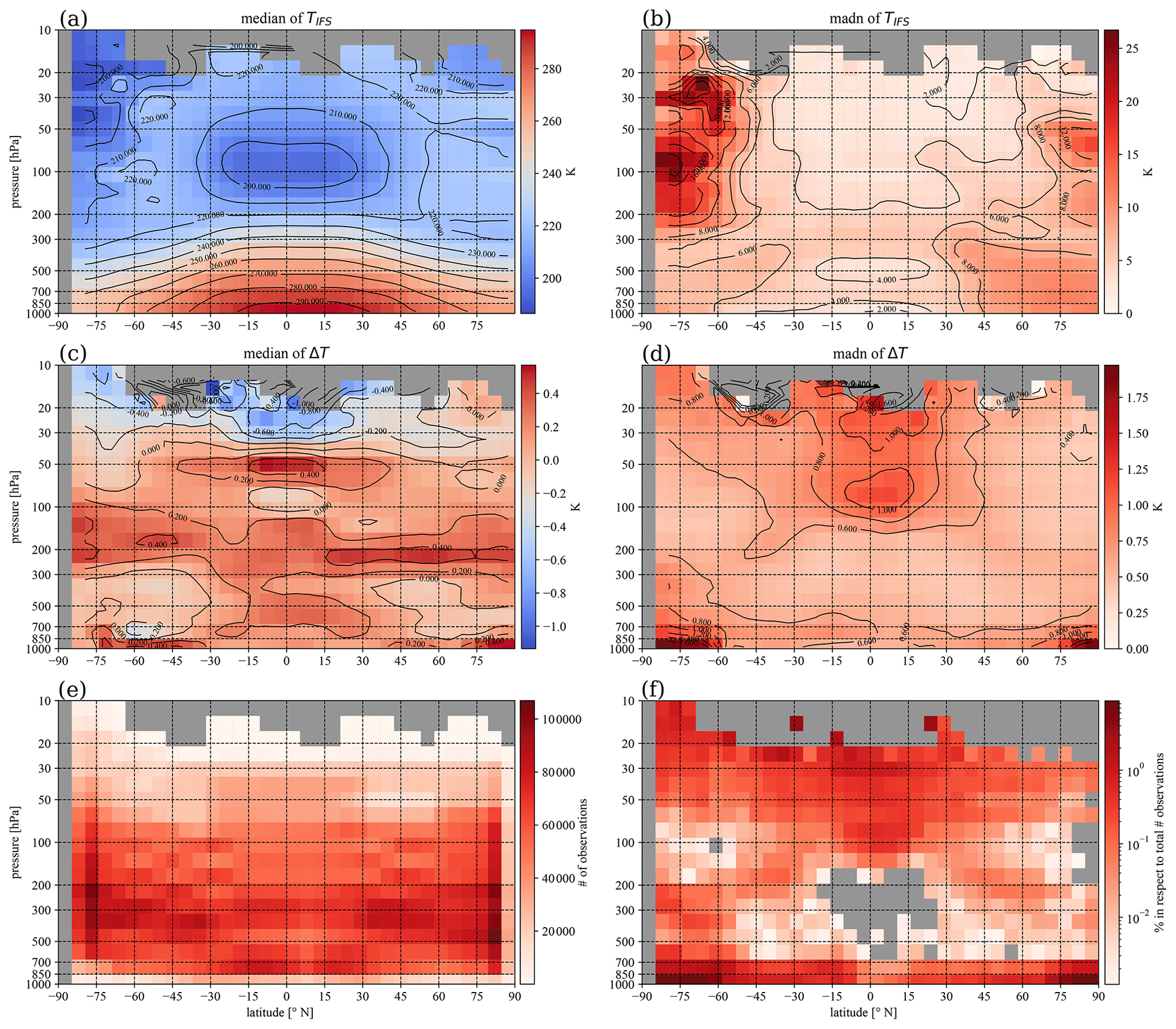
Figure 5The zonal and temporal statistics of the IFS temperature (a, b) and temperature differences between ARPEGE and IFS (c, d) computed for the same period as in Figs. 3–4. (a, c) The median and (b, d) madn=1.48mad are shown. In addition panel (e) shows the associated number of data for the statistics and (f) the number of samples found with a temperature difference ΔT>4 K used in the discussion of the Fig. 8.
A good consistency between model temperature fields is not only observed for the mean distribution. For 50 % of the distribution the differences remain below 1 K and 0.5 hPa almost everywhere below 30 km altitude (Fig. 4). For temperature this uncertainty is rather similar at all altitudes, although it is slightly larger in the stratosphere. A noticeable variability in temperature difference exists in the tropical stratosphere as shown in Fig. 5d. The largest amplitude in temperature difference, although spatially very localized, is observed near the ground over the two poles (Fig. 5d). Given that the chosen dataset describes primarily the Southern Hemisphere winter months, slightly increased variability is also observed to be high in the stratosphere over the South Pole (Fig. 5d). This is consistent with the largest variability in IFS model temperature observed over that area as shown in Fig. 5b. These regions, therefore, represent the most sensitive (in respect of temperature) areas for the HLOS retrieval in the studied period.

Figure 6Vertical cross-section of an Aeolus orbit extending over the area of South Indian Ocean, tropical Indian Ocean and Southeast Asia on 13 September 2019 at about 23:00 UTC. (a) A HLOSecmwf wind amplitude, (b) scattering ratio, (c) ΔT, i.e. a temperature difference between ARPEGE and IFS and the resulting (d) ΔHLOS as specified by Eq. (3). Note: dimensions of coloured boxes are symbolic, hence, not representing the area of representativeness of observations.
A scenario displayed in Fig. 6c presents the difference between two model temperature fields. Here data (each coloured box represents a valid observation) are extracted from a section of the Aeolus orbit crossing the regions of South Indian Ocean, tropical Indian Ocean and Southeast Asia. As shown in Fig. 6b several deep cloud systems exist on the path of Aeolus, increasing the lidar signal attenuation, as denoted by increased scattering ratio. In such situations temperature differences are found fairly consistent with the overall statistics shown in Fig. 5c; there is an overall positive ΔT along with vertical layers where ΔT becomes negative (e.g. especially above the tropical troposphere). Only few events of larger than 1–2 K are observed.
The largest deviations between the two NWP models can be further identified by analysing outliers of the difference probability density function (PDF) better shown in Fig. 4. Tails of the PDF are presented by the percentiles 0.5 and 99.5, which includes 99 % of data. It can be seen that model temperature difference will exceed about 2 K in the mid-troposphere and 3–4 K near the ground and in higher layers of troposphere and stratosphere for only 1 % of the distribution. For pressure this goes to about 1.5 hPa near the ground and decreases with altitude. In less than 1 % of cases, differences are even larger, although the overall summary of the results shown in Fig. 4 is that differences in temperature and pressure between the models are overall small.
The initial hypothesis assuming that statistical properties of the difference between two model forecasts can be used as a proxy of forecast errors is evaluated by a comparison against the ensemble spread of the ECMWF Ensemble of Data Assimilation (EDA) (Isaksen et al., 2010). Even though EDA does not provide information on long forecast range errors, the spatial patterns of the temporally averaged temperature forecast differences (Fig. 5) are relatively similar to those represented by the EDA temperature spread in Fig. 5a of Isaksen et al. (2010), supporting the experimental approach used in this paper. This qualitative comparison also shows that the EDA temperature spread in Fig. 5a of Isaksen et al. (2010) is typically twice as large as the median absolute difference of temperature differences reported in Fig. 5d with peak values around 2 K in the stratosphere. This factor is expected to be even larger since the EDA only describes short-range forecast errors.
Properties of the forecast differences displayed in Figs. 4–5 and sensitivities shown in Fig. 3 can be combined to estimate the largest expected HLOS variations due to the Rayleigh–Brillouin effect. The largest variations in HLOS are expected for temperature particularly in the stratosphere, due to larger HLOS sensitivity, but also near the ground, due to significant temperature differences between the two models. For an HLOS value of about 100 m s−1 the HLOS variations could exceed 0.6 m s−1 in less than 1 % of the situations. On the other hand the maximum expected variation of HLOS due to differences in pressure fields could be about 0.015 m s−1 at HLOS of 100 m s−1 but only near the ground (which is very unlikely) in less than 1 % of the cases. Therefore, the pressure component has no significant impact on the HLOS sensitivity and will not be analysed further.
4.3 Level-2B HLOS derived by using ARPEGE model temperature
By combining the HLOS sensitivity of the Rayleigh interferometer for Aeolus (Sect. 4.1) with temperature differences between ARPEGE and IFS models (Sect. 4.2), the HLOS correction (ΔHLOS as defined in Eq. 3) can be evaluated next.

Figure 7The ΔHLOS statistics related to the dataset presented in Figs. 3–5 and computed by Eq. (3). (a) The spatial and temporal statistics are displayed as a function of pressure showing the median, madn and several percentiles. The number of available data at specific pressure layers (solid green). (b) The 99th percentile of and (c) the median of the from the operational L2B output files.
Similar statistics as for ΔT are computed for ΔHLOS (Fig. 7). The spatial and temporal statistics lead to a symmetric PDF as shown in Fig. 7a, with madn larger than about 0.2 m s−1 above 30 hPa. The curve for the madn almost overlaps with the 75th percentile curve, which along with the 25th percentile presents 50 % of the distribution. Since a sensitivity ∂THLOS strongly depends on HLOS wind amplitude (Fig. 3), statistics for ΔHLOS should display this dependency. This is confirmed by Fig. 8a. Here the median is slightly larger only for HLOS winds larger than about 100 m s−1. On the other hand, several outliers with significantly larger values (up to more than 5 m s−1 – not shown) of ΔHLOS are observed. However, these outliers have no significant effect on the statistical properties of the ΔHLOS; in particular, 99.9 % of the distribution is still confined within the 1 % HLOS slope.

Figure 8(a) Statistics of L2B HLOS differences as a function of HLOSIFS wind. (b) Similar statistics but including only events associated with a temperature difference lower than 4 K in absolute values. Colour shading is associated with the density of events in a particular x–y area, with grey colour showing when data are not available. Several statistics are provided for a range of HLOS winds such as (solid black) median and (dotted black) madn. The two percentiles (dashed black) indicate the range of values included in 99 % (or 99.9 %) of the ΔHLOS distribution for a particular HLOS value, highlighting outliers. Blue denotes the 1 % (and 0.7 %) HLOS slopes used as a reference in the discussion.
The largest difference (i.e. 1 % of the PDF) in Fig. 7a exceeds 0.1 m s−1 below about 30 hPa and increases to about 0.4 m s−1 above. Although temperature differences are 99 % of the time smaller than about 4 K (Fig. 4a), the remaining 1 % of the distribution introduces differences of about several tens of kelvins. To better distinguish such outliers from the remaining distribution, statistics are re-evaluated for events with a temperature difference lower than 4 K (Fig. 8b). This simple filter efficiently removes all situations for which a relative difference %. The comparison between Fig. 8a and b reveals that the largest differences in HLOS are associated with the outliers of the temperature difference ΔT distribution. Figure 8b shows that over the whole range of HLOS values the difference ΔHLOS is well confined below a 1 % slope of HLOS and that in 99 % of situations it is well confined below a 0.7 % slope (i.e. ESA mission requirements).
The remaining question concerns the main characteristics of situations with ΔT>4 K. This can be discussed first by examining where such cases typically take place. Figure 5f displays the percentage of such cases relative to the total number of cases found in each latitude–pressure bin (i.e. Fig. 5e). The percentage shown in Fig. 5f is closely related to the madn of the ΔT shown in Fig. 5d. The largest contribution of the outliers (up to 10 % locally) is thus observed near the ground on both poles. A relatively large contribution is also noticeable in the tropical stratosphere, South Pole stratosphere (above ∼50 hPa) and around 200 hPa at latitudes 30–40∘ N/S. The latter is closely correlated with the position of the subtropical jet stream as can be confirmed by the median of IFS HLOS in Fig. 7c.
The largest values of ΔHLOS are produced by two mechanisms as is revealed by the outliers of the distribution displayed in Fig. 7b. First, the difference in HLOS is larger for in absolute larger HLOS winds, as is a consequence of the linear relation of ∂THLOS presented in Fig. 3a. This effect is confirmed by comparing it with the average HLOS shown in Fig. 7c. Thus, the largest differences in HLOS are expected near the location of subtropical jet streams. Due to the Southern Hemisphere winter months prevailing in the dataset, the stratosphere polar night jet is clearly evident over the South Pole (Fig. 7c). The second effect producing large values comes from the largest temperature differences (i.e. Fig. 5f). This contribution is the strongest near the ground over both poles, but it also contributes to increased HLOS differences in the tropical stratosphere and over the subtropical jet streams. Overall the largest relative differences are expected near the ground over both poles where the HLOS is on average small in absolute values.
The effect of, mainly, the first mechanism is well observed in the scenario displayed in Fig. 6d, taking into account associated temperature differences (Fig. 6c) and HLOS amplitude (Fig. 6a). The largest increments ΔHLOS are observed over the subtropical jet-stream regions (especially in the Southern Hemisphere) as well as in the tropical UTLS. In particular situation the largest differences in HLOS are found near the active deep cloud systems.
4.4 The contribution of the Mie contamination
The advantage of running L2Bp is that it allows the cross-validation of Eq. (3) and thus the estimation of the relative importance of the Mie contamination sensitivity term (i.e. in Eq. 2). To examine this contribution a second dataset is used (the FM-A period) to first produce the AUX_METecmwf and AUX_METmf files, and then L2Bp is run to generate HLOSecmwf and HLOSmf as described in Sect. 3, respectively. In addition, is computed using Eq. (3), with metadata provided from the L2B output of HLOSecmwf and ΔT, Δp from the two AUX_MET files. Taking into account Eqs. (1)–(2) and , the following equation can be derived.
where subscripts mf and ecmwf essentially define conditions of T, p, ρ and RR for which derivatives are computed. So, the difference between the methodology of Eq. (3) and L2Bp allows estimating properties of the contribution of the Mie contamination due to uncertain temperature and pressure information that affects the HLOS scattering ratio sensitivity term.
Since the FM-A dataset used here has not yet been officially reprocessed, it was first necessary to evaluate the sensitivity . Its properties have been found (not shown) very similar and consistent with the one from the FM-B dataset (i.e. Fig. 3a). In particular the slope of ∼0.002 K−1 is evident, although overall the sensitivity in FM-A dataset is for a value of about 0.05 smaller, which has been found small enough to be not significant for the rest of the study.
The Δ value has been found overall small as expected. Its PDF distribution is symmetric with values smaller than 0.05 m s−1 for 99 % of cases in absolute value for the dataset of interest. This suggests that the computation of correction using Eq. (3) compares well with the direct use of L2Bp in the particular case with the two AUX_MET files. This result suggests that in practice it is preferable to compute the HLOS correction using Eq. (3) when small differences in model temperature and pressure are expected, since it is faster and technically less demanding than rerunning the L2Bp using a different AUX_MET file. On the other hand, a portion of the distribution of Δ (i.e. 1 %) has been found having values of 0.4 m s−1 in absolute terms. These differences are a consequence of differences that arise in the HLOS sensitivity to scattering ratio evaluated with different atmospheric situations (i.e. temperature and pressure) as reflected by Eq. (4).
The Δ values are on average smaller than the HLOS differences due to temperature and pressure (i.e. ΔHLOS estimated by Eq. 3) as shown in Fig. 9. On average the HLOS sensitivity to scattering ratio brings an additional 10 %–20 % to HLOS correction when ΔHLOS>0.2 m s−1. The larger the value of ΔHLOS is, the smaller the relative contribution becomes. However, for large values of ΔHLOS, the amount of data used in the statistics becomes small (green line in figure), so the estimation is not significant, but this decreasing trend with increasing ΔHLOS is apparent. When ΔHLOS is small a value of Δ can increase up to about 70 % for the distribution median or even more than 100 % in about 1 % of cases. However, for small ΔHLOS values the overall correction to the HLOS correction is not of significant practical importance. Overall the sensitivity to scattering ratio is of less importance, even for the relatively large scatter ratio threshold of 1.6 used in the L2Bp, compared to the sensitivity to temperature.

Figure 9The relative contribution to the HLOS total correction of the HLOS sensitivity to the scattering ratio (Δ) compared to the contribution of the HLOS sensitivity to temperature and pressure (ΔHLOS). A complete description is given in Sect. 4.4. For each value on the x axis (bin spacing of 0.12 m s−1) statistics (median, 75th and 99th percentile) are presented together with the amount of data available (green solid line).
We conducted the sensitivity study on the Aeolus HLOS wind product to atmospheric temperature and pressure fields using the operational Aeolus data, ARPEGE model temperature and pressure short-term forecasts, and the Level-2B processor (L2Bp). The main goal was to evaluate the impact of the uncertainty in modelled temperature and pressure fields on the Rayleigh–Brillouin correction of the HLOS wind retrieval in L2Bp mainly from a perspective of data assimilation of HLOS winds in NWP. Two methods have been proposed. The first one estimates the possible HLOS correction through metadata provided by the operational L2Bp output files, and the second one consists of running the L2Bp locally at Météo-France.
The main assumption of the study has been that basic overall (e.g. time and zonally averaged) characteristics of NWP model temperature and pressure forecast uncertainties can be estimated by comparing atmospheric fields from two different global models (ARPEGE and IFS). For the L2B retrieval these uncertainties are propagated through the Rayleigh–Brillouin correction algorithm and also affect the Mie-contamination process. They reflect on the HLOS amplitude as an additional source to the random observation error. In comparison to the known Aeolus Rayleigh-clear HLOS observation errors, which is about 4 m s−1 (Martin et al., 2021), the uncertainty due to the Rayleigh–Brillouin correction represents only a small contribution. The main characteristic of this additional HLOS error distribution is that in 99 % of cases the HLOS amplitude differs by only 1 %, leading to a maximal difference of about 1 m s−1 for an HLOS wind value of 100 m s−1. On the other hand, in about 1 % of the cases the HLOS retrieval will differ by up to about 3 % with few cases having differences of several metres per second. These outliers are associated with temperature differences larger than about 4 K. The sensitivity to pressure is at least an order of magnitude less important and was not studied in detail. The overall small absolute differences in HLOS amplitude, which are in 99 % of cases less than 0.15 m s−1 and mostly located below 30 hPa, coming from model temperature and pressure uncertainties are in good agreement with expected values from the study of Dabas et al. (2008).
The largest differences in temperature between the two models over a 6-month period have been noticed over the poles near the surface which is believed to at least partly reflect differences in model orography as the ARPEGE model has a stretched horizontal grid with the highest resolution over Europe. On the other hand, differences in the lower to upper stratosphere and near the subtropical jet more realistically reflect on the forecast temperature errors linked to dynamical and physical processes. They are also expected to arise from differences in the two operational data assimilation systems and also because the two datasets represent different forecast lead times. The temporally and zonally averaged forecast error patterns are found to be fairly realistic, e.g. when compared to the spread of the ECMWF Ensemble of Data Assimilation (EDA) system as presented by Isaksen et al. (2010), comforting our initial assumption. However, their amplitudes are found underestimated for more than 50 % since the comparison of the two NWP datasets is affected by forecast error correlations due to similarities in the design of both NWP systems. This also affects the HLOS sensitivity, which is therefore expected to be overall underestimated. Despite this limitation, results showed how temperature forecast errors can impact the L2Bp HLOS wind retrieval.
By running the L2Bp using different temperature and pressure input information, it has been possible to study the impact of the uncertainty in modelled temperature and pressure on Mie-contamination HLOS correction. This correction is applied after the Rayleigh–Brillouin correction in the L2Bp. In particular the sensitivity of the HLOS to the scattering ratio reveals that the HLOS retrieval algorithm slightly differs for different atmospheric conditions. Results showed that this contribution brings about an additional 10 % error on top of the Rayleigh–Brillouin correction. Since the latter is already a small contribution to the HLOS error, the impact of the Mie-contamination correction sensitivity is not seen as a significant contribution.
The most appropriate option to quantify the sensitivity to temperature and pressure on HLOS retrievals is to use the best collocated information on temperature and pressure. The study mostly confirms the expected values from (Dabas et al., 2008), who showed the relatively small contribution of the temperature forecast errors (around 1–2 K for a 24 h forecast) to the overall HLOS error. However, results have highlighted the necessary quantification of the spatio-temporal variability of these errors that can be locally non-negligible. Since the current HLOS random observation errors from the Aeolus mission are significantly larger than expected due to a number of instrumental drawbacks, there is not much improvement to be expected from a better quantification of temperature forecast errors in L2Bp. Currently, the L2Bp assumes no error in temperature and pressure fields (provided by the IFS model), which, as shown by this study, appears to be a very good approximation for the purpose of NWP data assimilation of HLOS winds. However, it is recognized that uncertainties related to the Rayleigh–Brillouin corrections will become of more significance for the Aeolus follow-on missions where the quality of observations is expected to be improved. At the same time it is also recognized that forecast errors should decrease or be better quantified in the coming years, which again reduces the significance of this particular uncertainty in the HLOS retrieval.
The reprocessed Aeolus dataset of baseline 2B10 is publicly available at the ESA Aeolus dissemination system (https://aeolus-ds.eo.esa.int/oads/access/, ESA, 2020). The Aeolus data have been publicly available since May 2020.
The initial set-up of the experiment, the statistical analysis and the publication were prepared by MŠ. The framework for the production of the auxiliary meteorological files inside the ARPEGE data assimilation system was designed as a collaboration of MŠ, VP and CP. JFM supported the development of the method and analysis of the data and significantly contributed during the writing process of the publication. All co-authors engaged in the discussion leading to improvements in the publication.
The authors declare that they have no conflict of interest.
The results presented in Sect. 4.4 are preliminary since data that have been used are not yet publicly available since they have not yet been properly calibrated and validated.
Publisher's note: Copernicus Publications remains neutral with regard to jurisdictional claims in published maps and institutional affiliations.
This article is part of the special issue “Aeolus data and their application (AMT/ACP/WCD inter-journal SI)”. It is not associated with a conference.
The authors want to thank the ESA and DISC (Data, Innovation and Science Cluster) for the support and the provision of the preliminary datasets. We would especially like to thank Michael Rennie (ECMWF) and Jos De Kloe (KNMI) for their support and feedback during the study.
This research has been supported by the Centre National d'Etudes Spatiales (grant no. 5461-MTO-4500064868).
This paper was edited by Anne Grete Straume-Lindner and reviewed by two anonymous referees.
Courtier, P., Freydier, C., Geleyn, J.-F., Rabier, F., and Rochas, M.: The Arpege Project at Météo-France, in: Proc ECMWF Workshop, Numerical methods in atmospheric modelling, 9–13 September 1991, Shinfield Park, Reading, UK, ECMWF, vol. 2, 193–232, 1991. a
Dabas, A., Denneulin, M. L., Flamant, P., Loth, C., Garnier, A., and Dolfi-Bouteyre, A.: Correcting Winds Measured with a Rayleigh Doppler Lidar from Pressure and Temperature Effects, Tellus A, 60 A, 206–215, https://doi.org/10.1111/j.1600-0870.2007.00284.x, 2008. a, b, c, d, e, f, g
De Kloe, J., Stoffelen, A., Rennie, M., Tand, D., Andersson, E., Dabas, A., Poli, P., and Hubert, D.: ADM-Aeolus Level-2B/2C Processor Input/Output Data Definitions Interface Control Document, Documentation for Level-2B processor version 3.30, available at: https://confluence.ecmwf.int/display/AEOL/L2B+processor+documentation+and+datasets (last access: 17 May 2021), 2020. a
ESA: ADM-Aeolus Mission Requirements Document, Tech. Rep. EOP-SM/2047, ESA, available at: https://esamultimedia.esa.int/docs/EarthObservation/ADM-Aeolus_MRD.pdf (last access: 17 May 2021), 2016. a
ESA: Aeolus Online Dissemination System, available at: https://aeolus-ds.eo.esa.int/oads/access, last access: 27 November 2020. a
Gu, Z. and Ubachs, W.: A Systematic Study of Rayleigh-Brillouin Scattering in Air, N2, and O2 gases, J. Chem. Phys., 141, 1–11, https://doi.org/10.1063/1.4895130, 2014. a
Hersbach, H., Bell, B., Berrisford, P., Hirahara, S., Horányi, A., Muñoz-Sabater, J., Nicolas, J., Peubey, C., Radu, R., Schepers, D., Simmons, A., Soci, C., Abdalla, S., Abellan, X., Balsamo, G., Bechtold, P., Biavati, G., Bidlot, J., Bonavita, M., De Chiara, G., Dahlgren, P., Dee, D., Diamantakis, M., Dragani, R., Flemming, J., Forbes, R., Fuentes, M., Geer, A., Haimberger, L., Healy, S., Hogan, R. J., Hólm, E., Janisková, M., Keeley, S., Laloyaux, P., Lopez, P., Lupu, C., Radnoti, G., de Rosnay, P., Rozum, I., Vamborg, F., Villaume, S., and Thépaut, J.-N.: The ERA5 global reanalysis, Q. J. Roy. Meteor. Soc., 146, 1999–2049, https://doi.org/10.1002/qj.3803, 2020. a
Horanyi, A., Cardinali, C., Rennie, M., and Isaksen, L.: The Assimilation of Horizontal Line-of-Sight Wind Information into the ECMWF Data Assimilation and Forecasting System. Part I: The Assessment of Wind Impact, Q. J. Roy. Meteor. Soc., 141, 1223–1232, https://doi.org/10.1002/qj.2430, 2015. a
Isaksen, L., Bonavita, M., Buizza, R., Fisher, M., Haseler, J., Leutbecher, M., and Raynaud, L.: Ensemble of data assimilations at ECMWF, ECMWF technical memorandum, Number 636, https://doi.org/10.21957/obke4k60, 2010. a, b, c, d
Marseille, G.-J. and Stoffelen, A.: Toward Scatterometer Winds Assimilation in the Mesoscale HARMONIE Model, IEEE J. Sel. Top. Appl., 10, 2383–2393, https://doi.org/10.1109/JSTARS.2016.2640339, 2017. a
Marseille, G.-J., Stoffelen, A., and Barkmeijer, J.: A Cycled Sensitivity Observing System Experiment on Simulated Doppler Wind Lidar Data during the 1999 Christmas Storm “Martin”, Tellus A, 60 A, 249–260, https://doi.org/10.1111/j.1600-0870.2007.00290.x, 2007. a
Marseille, G.-J., Stoffelen, A., and Barkmeijer, J.: Impact Assessment of Prospective Spaceborne Doppler Wind Lidar Observation Scenarios, Tellus A, 60A, 234–248, https://doi.org/10.1111/j.1600-0870.2007.00289.x, 2008. a
Martin, A., Weissmann, M., Reitebuch, O., Rennie, M., Geiß, A., and Cress, A.: Validation of Aeolus winds using radiosonde observations and numerical weather prediction model equivalents, Atmos. Meas. Tech., 14, 2167–2183, https://doi.org/10.5194/amt-14-2167-2021, 2021. a, b, c
Matsushita, Y., Kado, D., Kohma, M., and Sato, K.: Relation between the interannual variability in the stratospheric Rossby wave forcing and zonal mean fields suggesting an interhemispheric link in the stratosphere, Ann. Geophys., 38, 319–329, https://doi.org/10.5194/angeo-38-319-2020, 2020. a
Reitebuch, O.: The Spaceborne Wind Lidar Mission ADM-Aeolus, in: Atmospheric Physics, Research Topics in Aerospace, edited by: Schumann, U., Springer, Berlin, Heidelberg, Germany, https://doi.org/10.1007/978-3-642-30183-4_49, 2012. a
Rennie, M. and Isaksen, L.: The NWP impact of Aeolus Level-2B Winds at ECMWF, ECMWF technical memorandum, Number 864, https://doi.org/10.21957/alift7mhr, 2020. a, b, c
Rennie, M., Tan, D., Andersson, E., Poli, P., Dabas, A., De Kloe, J., Marseille, G.-J., and Stoffelen, A.: Aeolus Level-2B Algorithm theoretical basis document – Mathematical description of the Aeolus Level-2B processor, Documentation for Level-2B processor version 3.30, available at: https://confluence.ecmwf.int/display/AEOL/L2B+processor+documentation+and+datasets (last access: 17 May 2021), 2020. a, b, c, d
Šavli, M., Žagar, N., and Anderson, J.: Assimilation of Horizontal Line-of-Sight Winds with a Mesoscale EnKF Data Assimilation System, Q. J. Roy. Meteor. Soc., 144, 2133–2155, https://doi.org/10.1002/qj.3323, 2018. a
Stoffelen, A., Pailleux, J., Kallen, E., Vaughan, J. M., Isaksen, L., Flamant, P., Wergen, W., Andersson, E., Schyberg, H., Culoma, A., Meynart, R., Endemann, M., and Ingmann, P.: The Atmospheric Dynamics Mission for Global Wind Field Measurement, B. Am. Meteorol. Soc., 86, 73–87, https://doi.org/10.1175/BAMS-86-1-73, 2005. a, b
Stoffelen, A., Marseille, G.-J., Bouttier, F., Vasiljevic, D., de Haan, S., and Cardinali, C.: ADM-Aeolus Doppler Wind Lidar Observing System Simulation Experiment, Q. J. Roy. Meteor. Soc., 132, 1927–1947, https://doi.org/10.1256/qj.05.83, 2006. a
Tan, D. G. H. and Andersson, E.: Simulation of the Yield and Accuracy of Wind Profile Measurements from the Atmospheric Dynamics Mission (ADM-Aeolus), Q. J. Roy. Meteor. Soc., 131, 1737–1757, https://doi.org/10.1256/qj.04.02, 2005. a
Tan, D. G. H., Andersson, E., Fisher, M., and Isaksen, L.: Observing-System Impact Assessment Using a Data Assimilation Ensemble Technique: Application to the ADM–Aeolus Wind Profiling Mission, Q. J. Roy. Meteor. Soc., 133, 381–390, https://doi.org/10.1002/qj.43, 2007. a
Tan, D. G. H., Andersson, E., De Kloe, J., Marseille, G.-J., Stoffelen, A., Poli, P., Denneulin, M. L., Dabas, A., Huber, D., Reitebuch, O., Flamant, P., Le Rille, O., and Nett, H.: The ADM-Aeolus Wind Retrieval Algorithms, Tellus A, 60A, 191–205, https://doi.org/10.1111/j.1600-0870.2007.00285.x, 2008. a
Tenti, G., Boley, C. D., and Desai, R. C.: On the kinetic model description of Rayleigh-Brillouin scattering from molecular gases, Can. J. Phys., 52, 285, https://doi.org/10.1139/p74-041, 1974. a
Weiler, F., Kanitz, T., Wernham, D., Rennie, M., Huber, D., Schillinger, M., Saint-Pe, O., Bell, R., Parrinello, T., and Reitebuch, O.: Characterization of dark current signal measurements of the ACCDs used on-board the Aeolus satellite, Atmos. Meas. Tech. Discuss. [preprint], https://doi.org/10.5194/amt-2020-458, in review, 2020. a, b
Weissmann, M. and Cardinali, C.: The impact of airborne Doppler lidar observations on ECMWF forecasts, ECMWF technical memorandum, Number 505, https://doi.org/10.21957/3zjzqeh1a, 2006. a
Weissmann, M., Langland, R. H., Cardinali, C., Pauley, P. M., and Rahm, S.: Influence of airborne Doppler wind lidar profiles near Typhoon Sinlaku on ECMWF and NOGAPS forecasts, Q. J. Roy. Meteor. Soc., 138, 118–130, https://doi.org/10.1002/qj.896, 2012. a
Wilks, D. S.: Statistical Methods in the Atmospheric Sciences, 3nd edn., Elsevier Academic Press, Cambridge, MA, USA, 2011. a
Witschas, B., Lemmerz, C., Geiß, A., Lux, O., Marksteiner, U., Rahm, S., Reitebuch, O., and Weiler, F.: First validation of Aeolus wind observations by airborne Doppler wind lidar measurements, Atmos. Meas. Tech., 13, 2381–2396, https://doi.org/10.5194/amt-13-2381-2020, 2020. a
Žagar, N.: Assimilation of Equatorial Waves by Line-of-Sight Wind Observations, J. Atmos. Sci., 61, 1877–1893, https://doi.org/10.1175/1520-0469(2004)061<1877:AOEWBL>2.0.CO;2, 2004. a
European Centre for Medium-Range Weather Forecasts (ECMWF) on 9 January 2019, Deutscher Wetterdienst (DWD) on 19 May 2020, Météo-France on 30 June 2020 and Meteorological Office (Met Office) on 8 December 2020