New correction method for the scattering coefficient measurements of a three-wavelength nephelometer

The aerosol scattering coefficient is an essential parameter for estimating aerosol direct radiative forcing and can be measured by nephelometers. Nephelometers are problematic due to small errors of nonideal Lambetian light source and angle truncation. Hence, the observed raw scattering coefficient data need to be corrected. In this study, based on the random forest machine learning model and taking Aurora 3000 as an example, we have proposed a new method to correct the scattering coefficient measurements of a three-wavelength nephelometer under different relative humidity conditions. The result shows that the empirical corrected values match Mie-calculation values very well at all three wavelengths and under all of the measured relative humidity conditions, with more than 85 % of the corrected values having less than 2 % error. The correction method obtains a scattering coefficient with high accuracy and there is no need for additional observation data.

1 Introduction

Atmospheric aerosol particles directly impact the Earth's radiative balance by scattering or absorbing solar radiation. However, the uncertainty of aerosol direct radiative forcing varies greatly, ranging between −0.77 and 0.23 W m⁻² (IPCC, 2013), which poses a great challenge for the accurate quantification of its effects on the Earth's climate system. Aerosol scattering and absorbing coefficients are the two most important parameters for estimating aerosol direct radiative forcing, and part of the estimation uncertainty comes from the inaccuracy in their measurements. Therefore, more precise measurements are needed. In recent years, two commercial integrating nephelometers (Aurora 3000 and TSI 3563) have been developed to measure aerosol scattering coefficients and hemispheric backscattering coefficients at three different wavelengths (450, 525, and 635 nm for the Aurora 3000 and 450, 550, and 700 nm for the TSI 3563). The three-wavelength integrating nephelometer is widely employed in field measurements and laboratory studies due to its high accuracy in measuring aerosol scattering coefficients (Anderson et al., 1996). However, it has two primary drawbacks – namely, the angle truncation and nonideal Lambertian light source – that contribute to a certain systematic error (Bond et al. 2009). The angle truncation indicates the lack of illumination near 0 and 180^∘ and the nonideal Lambertian light source means that the measured scattered signal is non-sinusoidal. The two drawbacks render the nephelometer measurement less precise.

In order to correct the measurement errors of the nephelometer, Anderson and Ogren (1998) used a single parameter as the scattering correction factor (CF) to quantify the nonideal effects. The CF is defined as the ratio of Mie-calculated scattering coefficient to that measured by the nephelometer and is closely related to the aerosol size and chemical composition. Müller et al. (2011) summarized several methods that have been proposed to derive the CF. Initially, researchers simulated the nephelometer measurements based on the Mie model. That is, they replaced the ideal sinusoidal function with the nephelometer's actual scattering angle sensitivity function to derive the scattering coefficient under nephelometer light source conditions. The scattering coefficient under the condition of ideal Lambertian light is also obtained by the Mie model, which allows calculation of the CF. However, this method additionally needs the particle number size distribution (PNSD), particle shape, and refractive index (Quirantes et al., 2008). It is not convenient to obtain simultaneous PNSD data because the measurement instrument is expensive and not easy to maintain.

An alternative popular correction mechanism is to constrain the CF simply by the wavelength dependence of scattering (scattering Ångström exponent, SAE). Considering that the SAE and CF both rely on particle size, Anderson and Ogren (1998) established a linear relationship between them for each TSI nephelometer's wavelength. This ingenious method is convenient because the scattering properties at different wavelengths, or SAEs, can be directly measured by the nephelometer itself. However, Bond et al. (2009) found that the SAE is also affected by the particle refractive index, while the CF is scarcely impacted by it. This difference renders the regression method less accurate. Furthermore, the absorption properties of sampled particles can alter the wavelength dependence of scattering, contributing to errors in this correction method for absorbing aerosols (Bond et al., 2009). Therefore, it is not an accurate correction method to establish a simple linear relationship between a single parameter SAE and CF.

In this study, the measurement limitations of angle truncation and the nonideal Lambertian light source are both considered. In light of the disadvantages of the methods mentioned above, we propose a new correction method for the scattering coefficient measurements of a three-wavelength nephelometer with the use of a machine learning model and taking an Aurora 3000 correction as an example. A description of the data and methodology under dry and other relative humidity conditions is given in Sect. 2. The verifications of the linear regression method and our new method are presented in Sect. 3. Finally, the conclusions are presented in Sect. 4.

2 Data and method

2.1 Site description

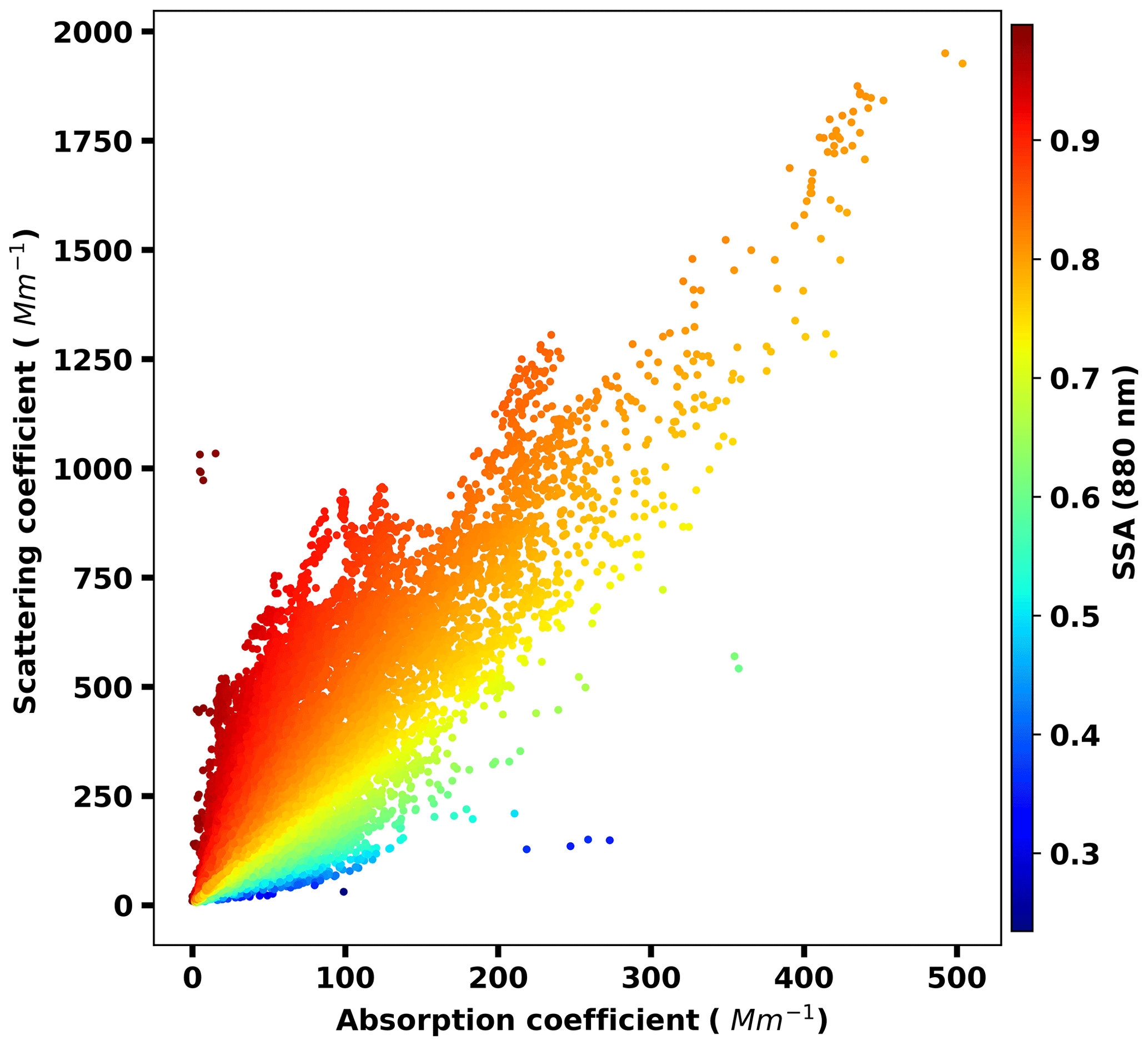
Eight field observations (Table 1) were conducted at different time periods in China, including two observations in Wuqing (39^∘38^′ N, 117^∘04^′ E), two in Xianghe (39^∘76^′ N, 117^∘01^′ E), and one observation in each of Wangdu (38^∘40^′ N, 115^∘08^′ E), Zhangqiu (36^∘71^′ N, 117^∘54^′ E), Beijing (39^∘59^′ N, 116^∘18^′ E), and Gucheng (38^∘9^′ N, 115^∘44^′ E). Five sites (Wuqing, Xianghe, Wangdu, Zhangqiu, and Gucheng) are located in suburban areas, representing the characteristics of regional anthropogenic aerosols in the North China Plain. Measurements in Beijing were conducted at Peking University (downtown Beijing), which is surrounded by two heavy traffic roads and hence it can well represent the typical case of urban pollution. The number size distribution measurements of the eight campaigns are obtained by a scanning mobility particle size (SMPS) or a twin differential mobility particle sizer (TDMPS) in conjunction with an aerodynamic particle sizer (APS), and the results cover a wide range of 10–1000 nm (Fig. 1). A 7-wavelength Aethalometer (Model AE33) and a Multi-Angle Absorption Photometer (MAAP) are utilized to measure black carbon mass concentration to derive the absorption coefficient. The single scattering albedo (SSA) of all field observations varies between 0.235 and 0.997 (Fig. 2).

Table 1 Summary of the eight field observations used in this paper.

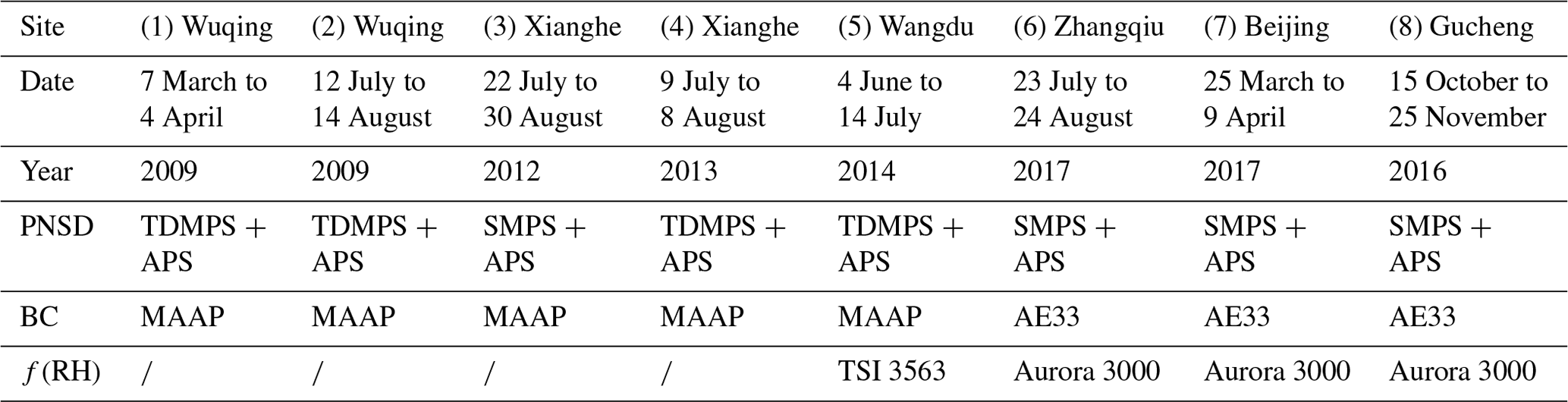
$/$: no f(RH) data obtained from that field observation.

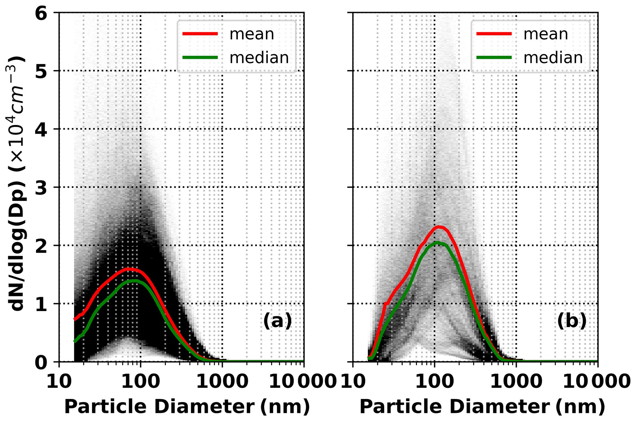
Figure 1 The number size distribution of the measured aerosol in (a) field observations (1)–(7) and (b) field observation (8).

Figure 2 The SSA of field observations (1)–(8).

2.2 Method

This paper proposes a simple and precise method of deriving the CF. Inspired by establishing a linear relationship between the SAE and CF (Anderson and Ogren, 1998; Müller et al., 2011), this paper first elucidates more parameters that exert impacts on the CF and can be directly obtained by nephelometer measurements. Considering the complex relationships among parameters and the requirements of the ordinary regression method (e.g., independent variables), it is not an appropriate means to use regression analysis to derive the relationship between the CF and some variables at each wavelength. Therefore, a random forest (RF) machine learning model from the scikit-learn machine learning library (Pedregosa et al., 2011), an effective method that can be used for classification and nonlinear regression (Breiman, 2001), is adopted. The RF model has several advantages (Zhao et al., 2018). First, it involves fewer assumptions of dependency between observations and results than traditional regression models. Second, there is no need for a strict relationship among variables before implementing the model simulation. Third, this model requires much fewer computing resources than deep learning. Finally, it has a lower over-fitting risk. Based on this machine learning model, our new method splits the above datasets into seven training datasets and one test dataset and then uses the Mie model and the training datasets to calculate the CF. The training dataset CFs, combined with parameters that impact the CF and can be directly obtained from nephelometer, are used to train the machine learning model. The derived RF models are verified by the test dataset. If the verification results are credible, the RF models can be directly used in field measurements to predict the in situ CF and finally obtain the corrected scattering coefficient.

2.2.1 Correction under dry conditions

An important feature of Mie scattering is that the larger the particle, the more forward scattering, meaning that the ratio of the backscattering coefficient to total scattering coefficient, or the hemispheric backscattering fraction (HBF), becomes smaller. Therefore, the HBF can to some extent stand for aerosol size and this paper aims to determine whether the HBF can be used as one parameter to predict the CF or not. Considering that both the SAE and CF relate to particle size, this paper uses the datasets of field observations (1)–(7) to explore the relationship between the CF and the calculated SAE and HBF at different wavelengths (Fig. 3).

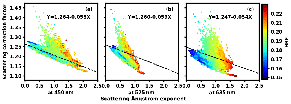
Figure 3 Scattering correction factors versus the scattering Ångström exponent. Panels (a, b, c) represent the results at the wavelengths of 450, 525, and 635 nm, respectively. The black dashed line is a statistical linear relationship and the color of the points represents the hemispheric backscattering fraction (HBF).

Following the method of Anderson and Ogren (1998) and Müller et al. (2011), we established a linear regression equation between the CF and SAE (black dashed lines). It is found that the change in the CF could be constrained by the change of the SAE to a certain extent, but the data points are dispersed from the regression equation. The larger the HBF, the greater the slope of the CF changes with the SAE. Therefore, besides the SAE, the HBF can be utilized to provide extra information on particle size and thus predict the CF.

Before establishing the relationship between the CF and the calculated SAE and HBF, it is necessary to obtain the size range for which particles contribute significantly to the variations of the SAE and HBF. This paper makes the assumption that there are three independent types of particle composition: scattering particles, absorbing particles, and core–shell mixed particles with a core radius of 35 nm. The refractive index is 1.80−0.54i (Ma et al., 2012) for the absorbing materials and $\mathrm{1.53}-{\mathrm{10}}^{-\mathrm{7}}i$ (Wex et al., 2002) for the scattering materials. Based on this assumption and all measured size distributions mentioned above, the variation of the SAE at the three wavelength combinations (450+525, 450+635, and 525+635 nm) and the HBF at the three wavelengths (450, 525, and 635 nm) in the particle size range (100 nm–10 µm) is calculated by the Mie model under the Aurora 3000 light source conditions (the light angle is limited from 10 to 171^∘; for details on the angular sensitivity function, please refer to Müller et al., 2011). Additionally, to distinguish the particle size range where the change of the SAE and HBF can be obviously manifested in the overall optical properties of aerosols, this paper also calculates the ratio of size-resolved scattering and hemispheric backscattering to total scattering for three types of assumed aerosols.

As shown in Fig. 4, for all three types of aerosols, scattering is mainly concentrated in the size range of 100–1000 nm; particles larger than 1000 nm contribute little to the total scattering and hence there is no followup discussion of the SAE change of these large particles. When particles are smaller than 1000 nm, the overall trend is that the SAE decreases with increasing particle size and that the SAE calculated at different wavelengths is obviously different. Especially when the particle is greater than 300 nm, the SAE variation with particle diameter is large, while particles in the size range of 100–300 nm contribute little to SAE variations. Therefore, the SAE variability is mostly sensitive to the concentration of particles in the 300–1000 nm size range.

Figure 4 The SAE change of scattering particles (a), absorbing particles (b), and core–shell mixing particles of core radius 35 nm (c) with the change in particle diameter (solid line). The dashed lines represent the ratio of scattering at a certain diameter relative to the total scattering.

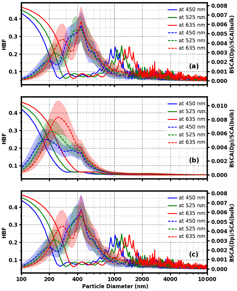
Figure 5 The HBF change of scattering particles (a), absorbing particles (b), and core–shell mixing particles of core radius 35 nm (c) with the change in particle diameter (solid line). The dashed lines represent the ratio of hemispheric backscattering at a certain diameter relative to the total scattering.

From Fig. 5, for environmental aerosol particles the backscattering of particles in the 100–1000 nm range also contributes a lot to the total scattering. The HBF characteristics of particles greater than 1000 nm is not discussed further. For particles with a size less than 300 nm, all three types of aerosol particles show a noticeable HBF variation with the change of particle size. However, particles larger than 300 nm contribute little to HBF variations. In other words, HBF variability is mostly sensitive to the concentration of particles in the 100–300 nm size range.

Based on the above analysis, it is known that the SAE and HBF can represent different size information of aerosol particles (300–1000 nm for the SAE and 100–300 nm for the HBF), and they are used together to derive the particle size information in the range of 100–1000 nm. Therefore, the SAE and HBF are two parameters that can be used for the machine learning process.

In order to calculate accurate SAEs and HBFs, scattering and backscattering information should be accurate. Considering that it is also affected by the mass concentration of BC and aerosol mixing states, not only PNSD but also black carbon (BC) data are needed to run the Mie model. According to Ma et al. (2012), when calculating the amount of externally mixed BC and core–shell mixed BC, R_ext is used to represent the ratio of the mass concentration of the externally mixed BC (M_ext-BC) to that of the total BC (M_BC):

$$\begin{array}{}\text{(1)}& R_{\mathrm{ext}}=M_{\mathrm{ext}\text{-}\mathrm{BC}}/M_{\mathrm{BC}}.\end{array}$$

Ma et al. (2012) pointed out that the HBF is sensitive to R_ext. Therefore, on the basis of the Mie model, we use PNSD, M_BC, and the assumed R_ext value to calculate the HBF. Next, the calculation of the HBF is compared with the observation results of nephelometers. If their difference is minimal, the assumed R_ext value is considered true. Deriving mass concentration of BC and PNSD data, assuming that the true R_ext is consistent at each size and there is no difference in the radius of BC core among core–shell mixed particles of the same size, we can calculate the number size distribution of core–shell mixed BC and externally mixed BC. Furthermore, the refractive index can also be obtained, making it possible to derive more precise information of scattering, backscattering, and then the SAE and HBF. Details about this method of retrieving PNSD and refractive indices can be found in Ma et al. (2012).

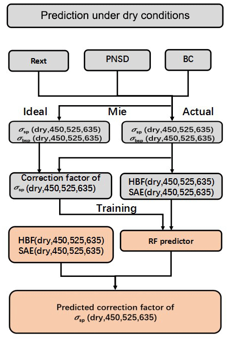
In summary, our nephelometer correction method under dry conditions encompasses the following procedure (Fig. 6):

1. Obtain information on particle number size distribution (PNSD), black carbon (BC), and mixing state (R_ext) of field observations (1)–(7).

2. Calculate the scattering and backscattering using the Mie model under the nephelometer light source conditions at the wavelengths of 450, 525, and 635 nm.

3. Calculate the hemispheric backscattering fractions (HBFs) at the three wavelengths.

4. Calculate the scattering Ångström exponent (SAEs) of the three wavelength combinations (450+525, 450+635, and 525+635 nm).

5. Calculate the scattering and backscattering using the Mie model under the ideal light source conditions at the wavelengths of 450, 525, and 635 nm.

6. Based on the results of the second and fifth steps, calculate the theoretical CF at the three wavelengths.

7. Use six parameters, including three HBFs and three SAEs, and the theoretical CF of each wavelength to train the machine learning model, which derives the RF predictor.

8. Verify the predictive validity of the trained model with the dataset of Gucheng.

Figure 6 Flow chart for estimating the CF under dry conditions by machine learning.

2.2.2 Correction under different RH conditions

Under elevated relative humidity conditions, a correction method taking the hygroscopicity into account is needed because, with the increment of relative humidity, the non-absorbing component in the aerosol particle can take up water due to its hygroscopic growth. Accordingly, the water content and particle size may change, resulting in a certain change in the CF for the same group of aerosol particles. Therefore, besides the SAE and HBF, more parameters related to hygroscopicity should be considered when deriving the CF under elevated relative humidity conditions.

The hygroscopicity or aerosol hygroscopic growth could be indicated by the scattering hygroscopic growth curve f(RH) and the backscattering hygroscopic growth curve f_b(RH). At low relative humidity, the growth due to an aerosol taking up water is weak and thus the change of f(RH) and f_b(RH) is small; as relative humidity goes up, the aerosol hygroscopic growth is obvious. Correspondingly, the change of f(RH) and f_b(RH) is large. Referring to research by Kuang et al. (2017) and Brock et al. (2016), the following formulas are used to describe f(RH) and f_b(RH):

$$\begin{array}{}\text{(2)}& {\displaystyle }f\left(\text{RH}\right)=\mathrm{1}+{\mathit{\kappa }}_{\mathrm{sca}}{\displaystyle \frac{\text{RH}}{\mathrm{100}-\text{RH}}},\text{(3)}& {\displaystyle }{f}_{\mathrm{b}}\left(\text{RH}\right)=\mathrm{1}+{\mathit{\kappa }}_{\mathrm{bsca}}{\displaystyle \frac{\text{RH}}{\mathrm{100}-\text{RH}}},\end{array}$$

where κ_sca and κ_bsca are fitting parameters representing the hygroscopic growth rate in aerosol scattering and backscattering.

When it comes to the aerosol overall hygroscopicity, according to 24 size distributions of κ obtained from Hachi field observations (Liu et al., 2014), this paper takes their average size distribution (the total volume-weighted κ is 0.281) as the basis. Next, in order to obtain a sequence of size distributions of κ, the basis κ is multiplied by values ranging from 0.05 to 2 with a 0.01 interval. According to the PNSD of outfield observations (1)–(7) and these assumed size distributions of κ, the theoretical Mie-calculation values are presented as scatter points in Fig. 7. On the basis of the above formulas, the lines represent fitted curves under nephelometer light source conditions. As can be seen for the three wavelengths, Eqs. (2) and (3) basically describe the trend of f(RH) and f_b(RH) values. In other words, aerosol scattering and hemispheric backscattering hygroscopic growth can be represented by parameters of κ_sca and κ_bsca. As a result, we wonder whether or not the hygroscopic growth of the CF (C(RH)) could be fitted similarly as the above formulas with parameter κ_c. The black scatter points in the figure do not lie close to the black dashed lines and, accordingly, the fit formula cannot accurately describe C(RH).

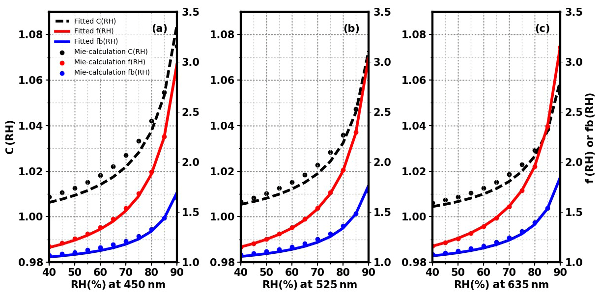
Figure 7 The comparison between κ fitted and theoretical Mie-calculation f(RH), f_b(RH), and C(RH) at the wavelengths of 450 nm (a), 525 nm (b), and 635 nm (c) under nephelometer light source conditions. The scatter points represent each theoretical Mie-calculation value. The red solid line is the f(RH) fitted curve and the blue solid line is the f_b(RH) fitted curve, both corresponding to the right ordinate value. The black dashed line is the C(RH) fitted curve, which corresponds to the left ordinate value.

Therefore, this paper attempts to derive the CF under different RH conditions in a similar machine learning way as described for the dry state. First of all, we need to find parameters impacting the CF under different RH conditions. Aerosol size accounts for the CF, as discussed in Sect. 2.2.1, and thereby the SAE and HBF in the dry state at three wavelengths are needed. In addition, hygroscopicity matters to a large extent. κ-Köhler theory (Petters and Kreidenweis, 2008) is thus applied, which uses hygroscopicity parameter κ to describe the hygroscopic growth of aerosol particles under different relative humidity conditions:

$$\begin{array}{}\text{(4)}& S={\displaystyle \frac{D^{\mathrm{3}}-D_{\mathrm{d}}^{\mathrm{3}}}{D^{\mathrm{3}}-D_{\mathrm{d}}^{\mathrm{3}}(\mathrm{1}-\mathit{\kappa })}}\cdot \exp \left({\displaystyle \frac{\mathrm{4}{\mathit{\sigma }}_{\mathrm{s}/\mathrm{a}}\cdot M_{\mathrm{water}}}{R\cdot T\cdot D\cdot g\cdot {\mathit{\rho }}_{\mathrm{w}}}}\right),\end{array}$$

where S is saturation ratio, D is the diameter of the aerosol particle after hygroscopic growth, D_d is the diameter of the aerosol particle in the dry state, ${\mathit{\sigma }}_{\mathrm{s}/\mathrm{a}}$ is the surface tension at the interface between the solution and air, T represents absolute temperature, M_water is the molar mass of water, R is the universal gas constant, and ρ_w is the density of water.

With the PNSD information, refractive index of the dry aerosol, mixing state, size distribution of κ, and water refractive index of $\mathrm{1.33}-{\mathrm{10}}^{-\mathrm{7}}i$ (Seinfeld and Pandis, 2006), on the basis of κ-Köhler theory (Eq. 4), this paper can calculate the aerosol optical parameters at different RH, which derives f(RH) and f_b(RH). Next, Eqs. (2) and (3) are used to fit the curve of f(RH) and f_b(RH) at each wavelength, thus deriving the fitting parameters κ_sca and κ_bsca, which can imply the size-resolved hygroscopicity. Combined with relative humidity, the estimated change in the CF with the relative humidity involves up to 13 physical quantities.

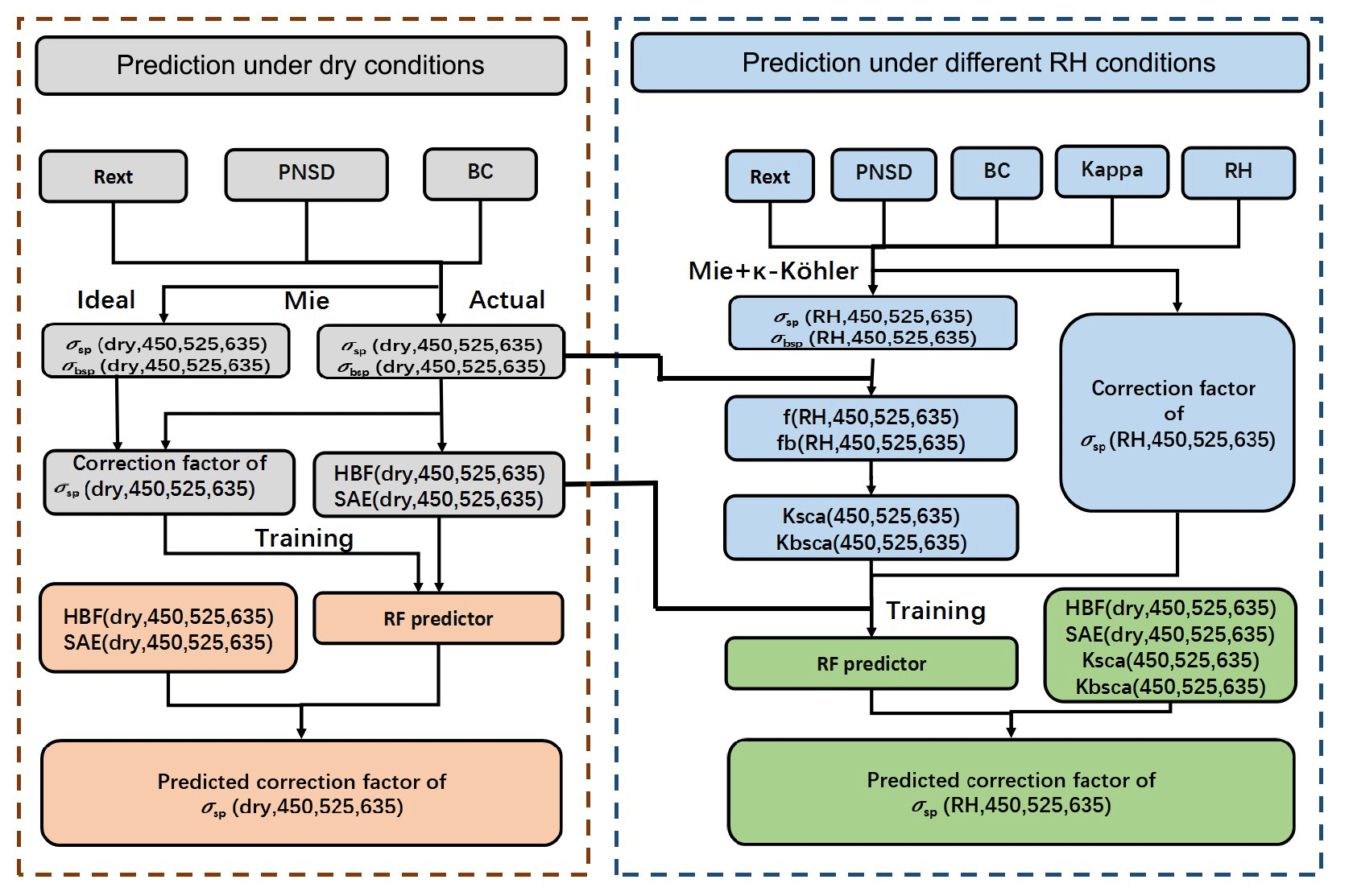
Figure 8 Flow chart for estimating the CF under different relative humidity conditions by machine learning.

To summarize, our nephelometer correction method under different relative humidity conditions encompasses the following procedure (Fig. 8):

1. Obtain information on particle number size distribution (PNSD), black carbon (BC), mixing state (R_ext), aerosol hygroscopicity parameter (κ), and relative humidity RH of field observations (1)–(7).

2. Calculate the scattering and backscattering using the Mie model under nephelometer light source conditions at the wavelengths of 450, 525, and 635 nm in the dry state.

3. Calculate the hemispheric backscattering fractions (HBFs) at the three wavelengths under dry conditions.

4. Calculate the scattering Ångström exponent (SAEs) of the three wavelength combinations (450+525, 450+635, and 525+635 nm) under dry conditions.

5. Under different relative humidity conditions and assumptions of aerosol hygroscopicity, according to the κ-Köhler theory, aerosol scattering and hemispheric backscattering after the hygroscopic growth are calculated on the basis of the nephelometer light source at three wavelengths.

6. Calculate f(RH) and f_b(RH) curves of the three wavelengths based on the scattering and hemispheric backscattering under dry and different relative humidity conditions.

7. Calculate the fitting parameters of κ_sca and κ_bsca from f(RH) and f_b(RH).

8. Calculate the scattering and hemispheric backscattering after the hygroscopic growth under ideal light source conditions at three wavelengths.

9. Based on the results of the fifth and eighth steps, calculate the theoretical CF at the three wavelengths.

10. Use 13 parameters, including three HBFs and three SAEs, relative humidity RH, three κ_sca and three κ_bsca at this RH, and the theoretical CF of each wavelength to train the machine learning model, which derives the RF predictor.

11. Verify the predictive validity of the trained model with the dataset of Gucheng.

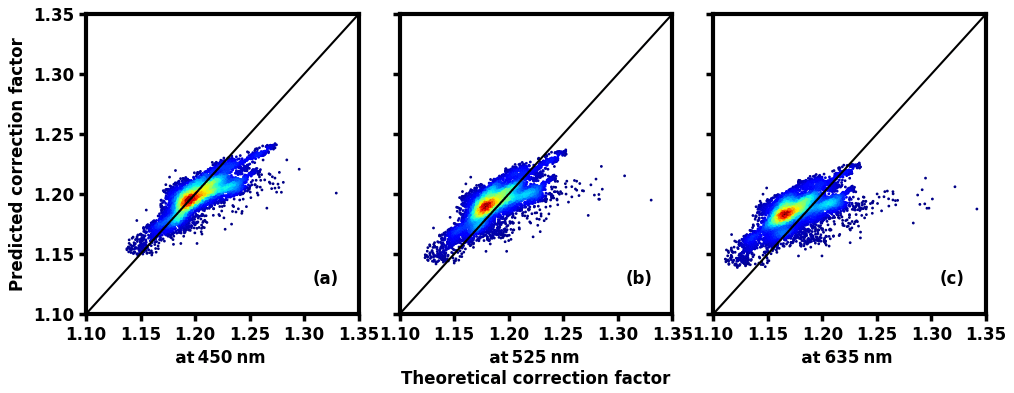
Figure 9 The comparison of theoretical correction factor and predicted correction factor calculated by the Ångström index at different wavelengths; panels (a, b, c) are the comparison results for 450, 525, and 635 nm, respectively. The black solid line represents that the theoretical correction factor equals the predicted one. The color of the data points represents the data density; the warmer the hue, the denser the data points.

3 Results and discussion

In order to verify the methods introduced above on the basis of Gucheng data and the derived RF predictor, we have predicted the CF and compared it with the theoretical Mie-calculated CF. First of all, for comparison, Gucheng data are used to verify the simple linear parameterization shown in Anderson and Ogren (1998) and Müller et al. (2011).

3.1 Verification of linear regression method

The PNSD and BC data of Gucheng are used to establish linear fit relationships between the CF and the corresponding SAE at three different wavelengths (450, 525, and 635 nm), which are, respectively, represented as:

$$\begin{array}{}\text{(5)}& {\displaystyle }\text{CF}=\mathrm{1.264}-\mathrm{0.058}\text{SAE},\text{(6)}& {\displaystyle }\text{CF}=\mathrm{1.260}-\mathrm{0.059}\text{SAE},\text{(7)}& {\displaystyle }\text{CF}=\mathrm{1.247}-\mathrm{0.054}\text{SAE}.\end{array}$$

As shown in Fig. 9, the CF ranges between 1.1 and 1.35. There is a relatively large gap between the predicted results derived from linear relationships and the theoretical simulation result, especially at the wavelengths of 525 and 635 nm.

When aerosols take up water due to hygroscopic growth with Gucheng data, this paper establishes different linear statistical relationships under different relative humidity conditions in order to estimate the CF. The data points gradually become dispersed from the 1:1 line as the relative humidity increases (Fig. 10). The reason is that under the condition of high humidity, the hygroscopic growth and thus particle size can vary greatly due to differences of aerosol hygroscopicity. Moreover, refractive indices also show large differences owing to the change of water content.

Figure 10 The comparison of theoretical correction factor and predicted correction factor calculated by the Ångström index at different wavelengths; panels (a, b, c) are the comparison results for 450, 525, and 635 nm, respectively. The black solid line represents that the theoretical correction factor equals the predicted one. The color of the data points represents different relative humidity conditions.

Therefore, the ordinary linear regression method of establishing a relationship between the CF and a single parameter SAE (Anderson and Ogren, 1998; Müller et al., 2011) cannot be applied to most cases, especially under the condition of high relative humidity.

3.2 Under dry conditions

When it comes to the results of our new method, as shown in Fig. 11 for 450 and 525 nm, the prediction performance is relatively good, and the correlation coefficient between prediction value and the theoretical Mie calculation is 0.88 and 0.84, respectively. More than 90 % of the points fall within the 2 % error range and most of them are basically concentrated near the 1:1 line. For 635 nm, the result is slightly worse, with the correlation coefficient at 0.76 and 85.88 % of the points within the 2 % error range. In general, compared with the traditional correction method, our method does not need to consider whether or not the aerosol has strong or wavelength-dependent absorption, which improves the accuracy of the CF estimation in the dry state; in addition, the input parameters can be obtained by the nephelometer's observation.

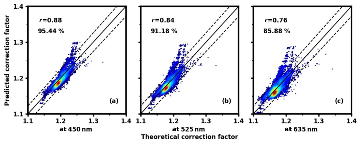
Figure 11 Under dry conditions, the comparison of the correction factors calculated by our method and the theoretical Mie-calculation values at the wavelengths of 450 nm (a), 525 nm (b), and 635 nm (c), respectively, with a black solid 1:1 line and two dashed lines representing a deviation of 2 %. The color of the data points represents data density; the warmer the hue, the denser the data point. r is the correlation coefficient, and the percentage indicates the percentile of points falling within the error range of 2 %.

3.3 Under different RH conditions

This paper uses each PNSD of the field observations (1)–(7) and averages them to plot Fig. 12, which represents the variation characteristics of the CF with the change of relative humidity and aerosol population hygroscopicity at the three wavelengths of 450, 525, and 635 nm, respectively.

Under all of the different relative humidity conditions, the CF at 450 nm is the largest, with that of 525 nm coming second, and that of 635 nm being the smallest (Fig. 12). All CFs at the three wavelengths increase with the increment of relative humidity. Furthermore, if the relative humidity remains constant, the CF also increases as aerosol hygroscopicity increases. This is reasonable since the environment relative humidity and the hygroscopicity of aerosols have positive impacts on particle sizes and thus the CF.

Figure 12 The theoretical calculation of the scattering correction factors (CFs) versus relative humidity (RH) and hygroscopicity κ at the wavelengths of 450 nm (a), 525 nm (b), and 635 nm (c). The dashed line represents a scattering correction factor in the dry state and the color represents the overall hygroscopicity of aerosols (κ). The color bar is derived from multiplying the total volume-weighted κ of 0.281 by values ranging from 0.05 to 2 with a 0.01 interval.

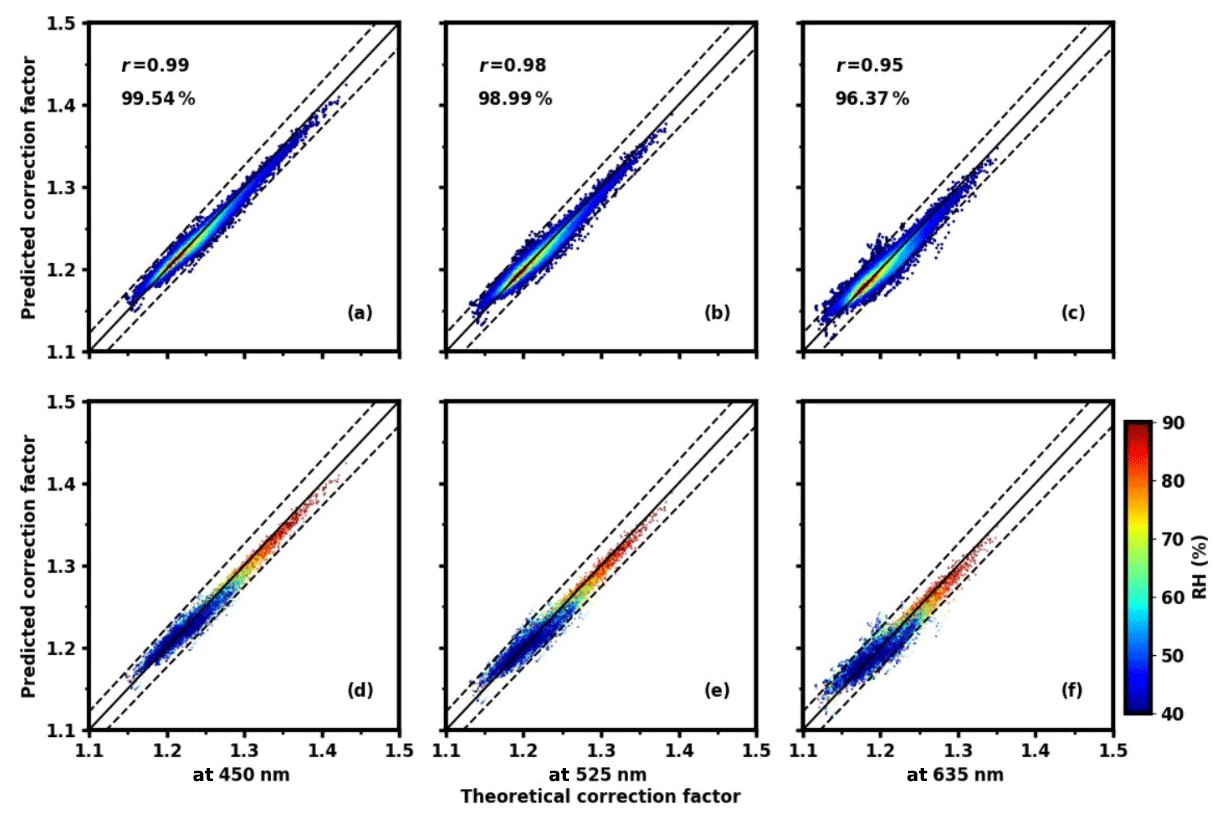
Figure 13 At different relative humidity conditions, the comparison of the correction factors calculated by our method and the theoretical Mie-calculation values at the wavelengths of 450 nm (a), 525 nm (b), and 635 nm (c), respectively, with a black solid 1:1 line and two dashed lines representing a deviation of 2 %. The color of the data points represents data density; the warmer the hue, the denser the data point. r is the correlation coefficient, and the percentage indicates the percentile of points falling within the error range of 2 %. The data in (d, e, f) are the same as those in (a, b, c), but the color here stands for different relative humidity conditions rather than density.

Our correction method under different RH conditions takes the humidity and hygroscopicity into account. As depicted in Fig. 13, the new method predicts the CF very well at all the three wavelengths, and nearly all scatter points at the three wavelengths are centered near the 1:1 line. For the 450 nm wavelength, the correlation coefficient between the prediction value and the theoretical Mie calculation reaches 0.99, with 99.54 % of the points falling within the error range of 2 %. For the 525 nm wavelength, the correlation coefficient is 0.98, with 98.99 % of the points falling within the error range of 2 % and for the 635 nm wavelength, the correlation coefficient is 0.95, with 96.37 % of the points in error by less than 2 %. From Fig. 13d–f, the new method's estimation of the CF is basically consistent in accuracy at each relative humidity. Another advantage of our new method is that all these input parameters can be obtained by the nephelometer's observation, achieving the goal of self-correction.

4 Conclusions

The aerosol scattering coefficient is an essential parameter for estimating aerosol direct radiative forcing, which can be measured by nephelometers. However, nephelometers have the problems of a nonideal Lambertian light source and angle truncation and hence the observed scattering coefficient data need to be corrected. The scattering correction factor (CF) is thus proposed and it depends on the aerosol size and chemical composition. The most direct calibration method is to combine the particle number size distribution, black carbon data, and Mie scattering model to correct the nephelometer. However, this method requires auxiliary measurement data. After proposing this method, the scattering Ångström exponent (SAE) measured by nephelometer itself is utilized to establish a linear relationship with the CF. After verification, it is found that the method lacks precision and accuracy. Therefore, our paper has proposed a new method of nephelometer self-correction.

Under dry conditions and after the analysis, the SAE and HBF can represent different ranges of aerosol particle size information (300–1000 nm for the SAE and 100–300 nm for the HBF). With the use of the existing observation results of PNSD, black carbon, and R_ext to obtain the SAE and HBF, this paper applies the random forest (RF) machine learning model to establish the relationship between the CF and the calculated SAE and HBF, and ultimately derives the trained RF model. With the dataset of Gucheng, the verification results show that this method is relatively accurate. The commonly used integrating nephelometer can derive in situ scattering and backscattering coefficients at three wavelengths to calculate three SAEs and three HBFs. Therefore, with the use of the derived RF model and the nephelometer calculation of the SAE and HBF, the CF could be predicted by the nephelometer itself.

Under other relative humidity conditions, the humidified nephelometer system is utilized. In addition to the dry aerosol particle size information, we should also consider the change in water content and particle size brought by the growth of aerosol taking up water. This paper finds that the CF increases with the increment of relative humidity and aerosol hygroscopicity. Therefore, on the basis of κ-Köhler theory, the existing observation results of PNSD, black carbon, R_ext, aerosol hygroscopicity parameter κ, and relative humidity are used to run the Mie model, obtaining the theoretical CF and 13 quantities relating to the CF change under different RH conditions. Similarly, the machine learning model is trained to obtain the relationship between the CF and the 13 quantities. With the dataset of Gucheng, the verification results show that the accuracy of the CF obtained by this method is very high. The humidified nephelometer system can observe scattering and hemispheric backscattering coefficients at three wavelengths under both dry and elevated RH conditions, obtaining the corresponding f(RH) and f_b(RH) under the nephelometer light source conditions. As a result, all 13 quantities, including six physical quantities of SAEs and HBFs representing dry aerosol size at each wavelength, six fitting parameters κ_sca and κ_bsca representing particle size-resolved hygroscopicity at each wavelength, and the relative humidity, can be directly obtained from nephelometers. Therefore, with the use of the derived RF model and the above 13 quantities, the CF could be predicted in situ by the humidified nephelometer system.

The strengths of our new method are summed up as follows: under either dry or any other relative humidity conditions, the prediction performance of the CF at three wavelengths is excellent. Furthermore, at each relative humidity, the accuracy of the CF estimation is almost the same. All inputs can be obtained through the nephelometer's observations, thus achieving self-correction; that is, on the basis of ensuring the accuracy of correction, there is no need for other aerosol microphysical observations.

Due to the limitations of Mie theory, our method cannot be applied to analyze datasets that include desert and marine aerosols and hence further studies are needed. In this study, the new method is put forward only based on datasets in the North China Plain. There might be errors in applying our RF models to predict the CF all over the world. Therefore, more field observation datasets are needed to verify and perfect this method, hopefully establishing a database of RF models in the future.