the Creative Commons Attribution 4.0 License.
the Creative Commons Attribution 4.0 License.
 | 16 Jul 2021
Estimating the optical extinction of liquid water clouds in the cloud base region
David P. Donovan
Herman W. J. Russchenberg
Accurate lidar-based measurements of cloud optical extinction, even though perhaps limited to the cloud base region, are useful. Arguably, more advanced lidar techniques (e.g. Raman) should be applied for this purpose. However, simpler polarisation and backscatter lidars offer a number of practical advantages (e.g. better resolution and more continuous and numerous time series). In this paper, we present a backscatter lidar signal inversion method for the retrieval of the cloud optical extinction in the cloud base region. Though a numerically stable method for inverting lidar signals using a far-end boundary value solution has been demonstrated earlier and may be considered as being well established (i.e. the Klett inversion), the application to high-extinction clouds remains problematic. This is due to the inhomogeneous nature of real clouds, the finite range resolution of many practical lidar systems, and multiple scattering effects. We use an inversion scheme, where a backscatter lidar signal is inverted based on the estimated value of cloud extinction at the far end of the cloud, and apply a correction for multiple scattering within the cloud and a range resolution correction. By applying our technique to the inversion of synthetic lidar data, we show that, for a retrieval of up to 90 m from the cloud base, it is possible to obtain the cloud optical extinction within the cloud with an error better than 5 %. In relative terms, the accuracy of the method is smaller at the cloud base but improves with the range within the cloud until 45 m and deteriorates slightly until reaching 90 m from the cloud base.
- Article
(2537 KB) - Full-text XML
- BibTeX
- EndNote


Lidar has been used to probe the atmosphere ever since 1960 (e.g. Collis, 1966; Fiocco and Smullin, 1963). Lidar measurements facilitate characterisation of the atmosphere and have many different applications, including determining the properties of aerosols (Müller et al., 1998) and clouds (Turner, 2005).
Lidars possess a unique ability to observe the optical properties of clouds, such as the cloud extinction coefficient (α). Through an inversion of the backscattered power received by a lidar system, an estimate of the cloud extinction coefficient can be retrieved (Klett, 1981). This optical property of the cloud can be linked to the cloud's microphysical properties (Kokhanovsky, 2004). Although lidar can only penetrate a small part of a cloud, typically 100 to 300 m from the cloud base, the cloud base region is of strong interest for studies concerned with cloud formation and aerosol–cloud interactions (McComiskey and Feingold, 2012).
Despite the long history of lidar measurements and the vast amount of data available, very few quantitative evaluations of the cloud optical extinction retrieval accuracy under realistic conditions exist (e.g. Carnuth and Reiter, 1986; Rocadenbosch et al., 1998). Lidar signal inversion in realistic conditions is more difficult due to the effects of finite lidar range resolution and multiple scattering occurring within the cloud.
In this paper, we present a procedure to retrieve the cloud optical extinction coefficient, using a single field of view (FOV) depolarisation lidar. We use the Klett solution (Klett, 1981) with the inclusion of a multiple scattering correction (Hu et al., 2006; Roy and Cao, 2010) and an explicit treatment of the molecular and cloud contributions to the returned signal (Fernald, 1984). We demonstrate, using synthetic lidar signals generated using a Monte Carlo RT model fed with large eddy simulation (LES) fields, that useful extinction profiles can be retrieved using simple elastic polarisation lidars.
The outline of the paper is as follows. In Sect. 2 we present background material. In Sect. 3 we give a brief description of the EarthCARE Simulator (ECSIM) and the scenes created for this investigation. Section 4 presents the results of the inversion, discusses the issues related to conducting accurate inversions, and presents our methodology to address them. We conclude the paper with a summary of the findings and an outlook of possible applications.
The single-scattering lidar equation for a two-component atmosphere (cloud and molecular) can be defined as follows:
where z is the altitude, P(z) is the received power as a function of altitude, Clid is the lidar calibration constant, βπ is the atmospheric backscatter coefficient, α is the atmospheric extinction coefficient, and the “c” and “m” subscripts distinguish between cloud and molecular backscatter and extinction (Fernald, 1984). As the Klett solution applies strictly to a one-component atmosphere, we introduce α′ and P′ in order to account for the mixed contributions from cloud and/or aerosol and molecular scattering (Fernald, 1984).
If we define the following:
where S is the cloud extinction-to-backscatter ratio (), then, in the following:
Thus, Eq. (1) can be recast as follows:
which has the general form of the single-component lidar equation and has a well-know solution form (Klett, 1981).
In order to calculate the two-component transformed optical cloud extinction coefficient, α′, we invert Eq. (1) following the analytical solution to the single-scattering lidar equation proposed by Klett (1981).
where, in the following:
α0 is the extinction coefficient at a reference height z0, and S is assumed to be range-independent within the cloud, and for water clouds and wavelengths in the range from 200 to 1064 nm, it is around 16 sr (Yorks et al., 2011). Following the method established by Klett (1981) and later Fernald (1984), we estimate the value of the extinction coefficient at the far end of the range interval to retrieve the full profile of the extinction coefficient. This method was tested for cloudy and foggy conditions and proved appropriate for retrieving the extinction values. It shows a small dependence on the estimated extinction boundary value () when the optical thickness of the range interval is increasing (Klett, 1985; Carnuth and Reiter, 1986).
Although the principle of this method of lidar signal inversion is straightforward, there are a number of issues that must be addressed to ensure accurate results. Section 4.1 outlines these difficulties and presents possible ways of overcoming them. In this work, we make use of simulated lidar signals for which the true extinction profiles are know. The simulations include the effects of realistic cloud structure and the effects of finite lidar range resolution and lidar multiple scattering. Each of these factors must be accounted for before accurate results can be produced by applying Eq. (5). Each of these issues is addressed in turn. In Sect. 4.1.3, we discuss the effects of finite range resolution, and in Sect. 4.1.2, the approach to accounting for multiple scatterings is discussed.
To evaluate the retrieval of the cloud extinction, we use synthetic signals produced using the EarthCARE simulator (ECSIM). ECSIM is a tool to simulate the measurements of four instruments, namely the 94 GHz cloud profiling radar, the high spectral resolution lidar at 353 nm, the multi-spectral imager, and the broadband radiometer (Donovan et al., 2015). The lidar model takes into account polarisation, multiple scattering, and the effects of finite lidar range resolution. For the simulations carried out in this work, the lidar wavelength was 355 nm, the field of view was 2 mrad, the laser divergence 0.1 mrad, and the range resolution was 15 m. The ECSIM radar model was also used in this paper in an ancillary role. To retrieve information about the cloud extinction, we only need information from lidar. However, information from radar can be used for a further analysis of the scene. Radar can add the ability to identify regions of drizzle. It can also penetrate through a liquid water cloud and, hence, is useful for establishing the height of the cloud top.
To create the scene used in this work, a liquid water content (LWC) field was generated by a LES and introduced to ECSIM. The LES case used corresponded to one from the FIRE campaign (Albrecht et al., 1988). The ECSIM simulation specifically used an output from the Dutch Atmospheric LES model (DALES; Heus et al., 2010). DALES utilises a two-moment bulk scheme to model precipitation (Khairoutdinov and Kogan, 2000), where condensed water is qualified as either cloud water or precipitation, and the number density of cloud droplets is prescribed. The ECSIM scene is created based on a snapshot of parameters extracted from DALES. Those parameters include temperature, pressure, non-precipitable cloud water, precipitation water content, and precipitation droplet number density. Furthermore, an explicit droplet size distribution (DSD) is needed to create an ECSIM scene. As DALES does not provide DSDs, imposed DSDs were used based on the DALES output. The precipitation mode DSD was based on the one from Khairoutdinov and Kogan (2000). The cloud mode DSDs were found by assuming modified gamma type distribution with a width parameter of 5 and assuming a constant cloud number density; the effective radius of the distributions was then calculated using the model LWC fields.
Figure 1 presents the cross section of the radar reflectivity factor and the attenuated backscatter coefficient of the used cloud scene. This cloud scene consists of 450 profiles of attenuated backscatter coefficient; all of those profiles were used in the analysis hereafter. We performed two simulations based on the same DALES output. One of the cloud scenes was made to simulate attenuated backscatter coefficient with the inclusion of single and multiple scattering effects (referred to as BMS later in the text), and the second simulation was made for only the single scattering attenuated backscatter coefficient (referred to as BSS later in the text). This allowed us to directly compare the impact of the multiple scattering on the retrieved values of the extinction coefficient and evaluate the correction for the multiple scattering presented in Sect. 4.1.2.
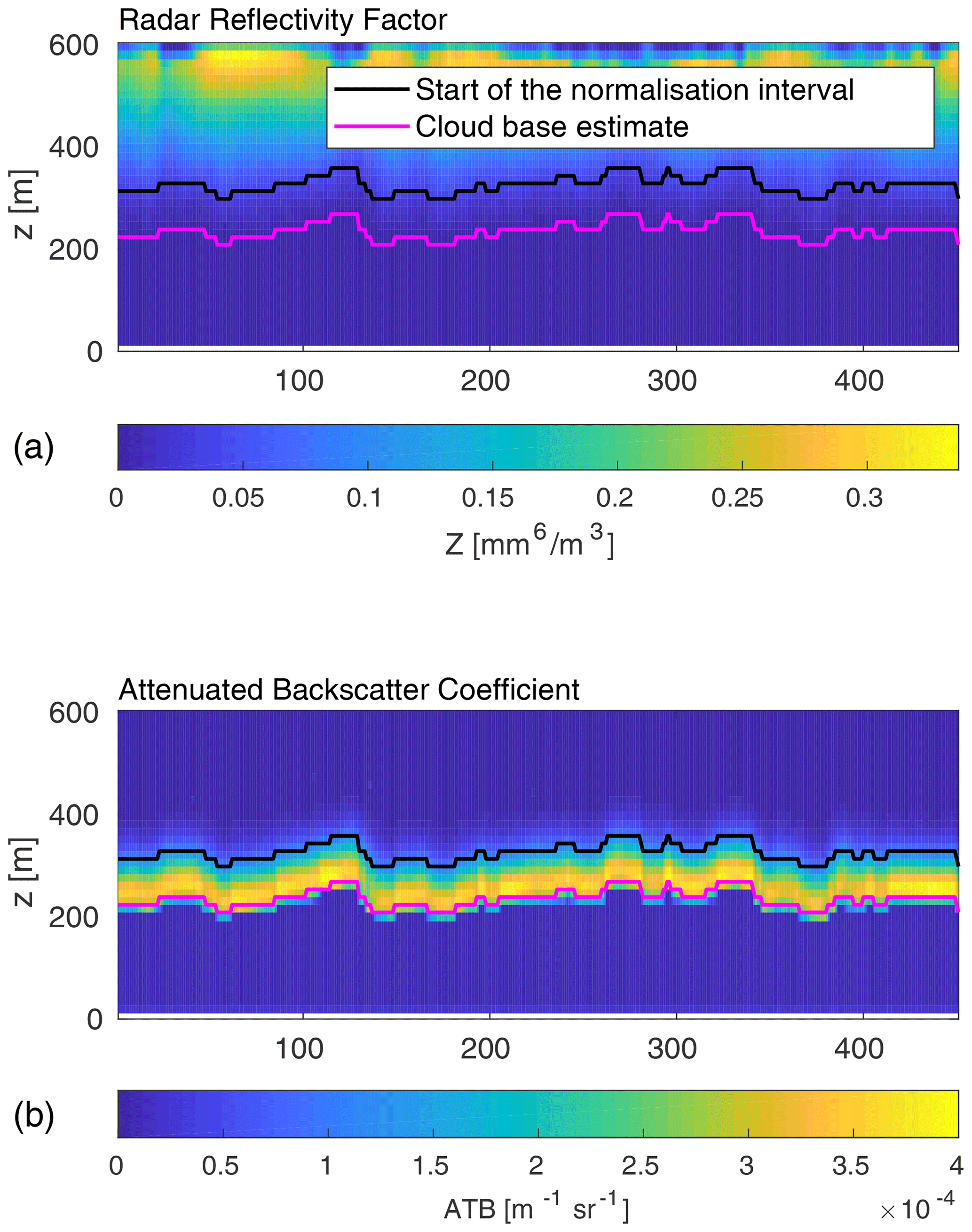
Figure 1Cross section of the radar reflectivity factor (a) and attenuated backscatter coefficient (b) of the cloud scene produced with the ECSIM simulator. The magenta line indicates the estimate of the cloud base height, and the black line indicates the beginning of the normalisation interval.
4.1 Difficulties in inversion steps
4.1.1 Defining the normalisation interval
In order to obtain a profile of the optical cloud extinction from lidar returns, we need to invert the received power (Eq. 1) into a cloud optical extinction coefficient, as explained in Sect. 2. Following the solution proposed by Klett (1985), it is necessary to define the range interval where the signal can be normalised. The value of extinction, , is estimated at a certain height, z0, based on the slope of the least square straight line fitted to the curve ATB = ATB(z). The value of is calculated as follows:
where ATB is the attenuated backscatter coefficient (ATB(z)=P(z)z2), and dz is the range resolution. Figure 2 presents the profile of the cloud optical extinction retrieved based on the slope method. It shows clearly that the slope method is not accurate at the cloud base, and the retrieved values come closer to the true extinction only at a certain height within the cloud. This is in accordance with a proposition by Klett (1981), who postulated that the normalisation height z0 where the value of is estimated should be located at the far end of the cloud. It should be noted that, in the approach presented in this paper, the cloud optical extinction obtained through the slope method is used only to retrieve the value of and initiate the inversion.
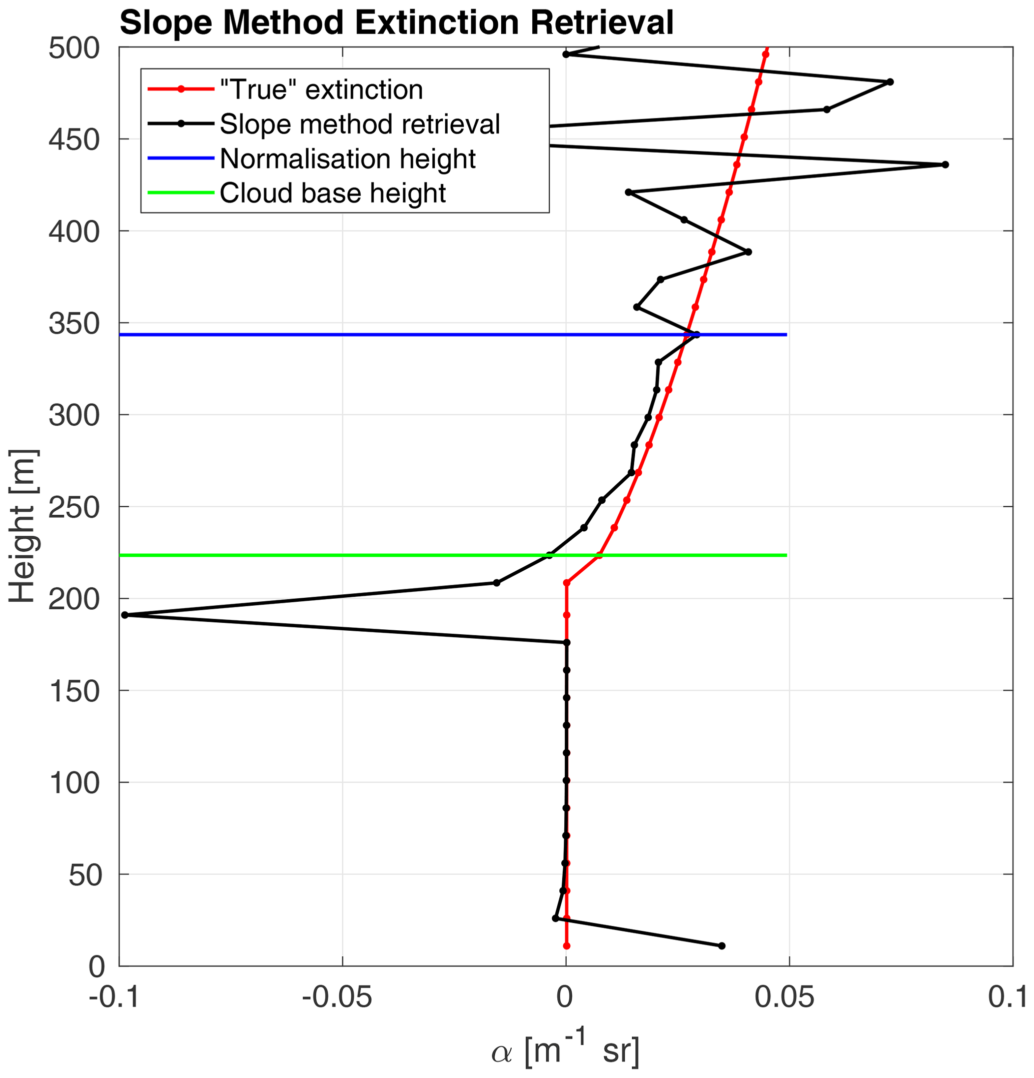
Figure 2Profile of the extinction coefficient retrieved based on the slope method (Eq. 7) and the true extinction profile calculated from ECSIM.
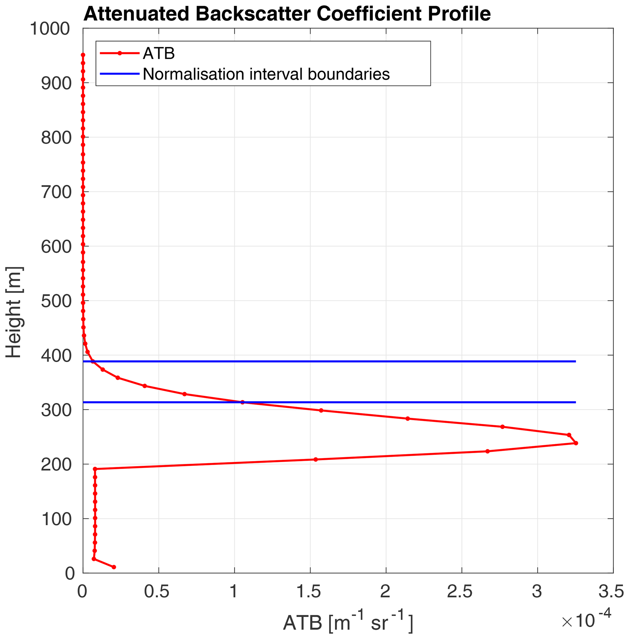
Another important aspect in deciding on the height of the normalisation interval is the profile of the attenuated backscatter coefficient (ATB). In order to calculate , ATB at the chosen height has to be still usable, meaning that the noise level cannot be too high. Figure 3 presents the signal profile with a marked normalisation interval. Note that the interval is above the peak of the signal and just before signal starts to be noisy or lost. In this study, we chose a threshold for the ATB usability in the normalisation interval at a signal-to-noise ratio (SNR) of 20. We tested the sensitivity of the inversion method to different values of SNR and found that values below 20 tend to influence the retrieval in the higher parts of the cloud. The first four bins within the cloud (up to 60 m within the cloud) are only affected by a mean error increase of 3 %. If the SNR is below 20, then the normalisation interval has to be set at a lower height.
4.1.2 Correcting the multiple scattering
Measurements of water clouds by lidar backscatter always involve some contribution from multiple scattering. In this study, we use the multiple scattering correction based on the accumulated depolarisation ratio (δacc) introduced by Hu et al. (2006) and further demonstrated by Cao et al. (2009). Lidar multiple scattering occurring in water clouds can be linked to the depolarisation ratio. At 180∘ backscatter direction, the single scattering of spherical droplets retains the polarisation of the incident light. However, scattering at different scattering angles changes the polarisation state. For the liquid water clouds, the depolarisation of the signal can be attributed to the multiple scattering (Sassen and Petrilla, 1986).
Based on the above-described characteristics of water clouds and lidar backscatter, Hu et al. (2006) described a relation between the linear depolarisation of the backscatter signal and the fraction of multiple scattering present in that signal. Based on the Monte Carlo simulations of the multiple scattering signals for numerous scenarios and different fields of view, they derived the following relation:
where IS(z) is the integrated, range-corrected single scattering signal, and IT(z) is the integrated, range-corrected total scattering signal (single and multiple scattering). Both signals are integrated between the cloud boundaries, where the cloud base height is established based on the lidar measurements. We use the top of the normalisation interval instead of the cloud top, as measurements above that height are no longer relevant. δacc(z) is the accumulated depolarisation ratio. It can be calculated from the parallel and perpendicular components of the total backscattering signal as follows:
where is the total integrated perpendicular backscattered signal, and is the total integrated parallel backscattered signal.
In order to calculate the signal corrected for the multiple signal, in other words, the signal contributing only to the single scattering ATBSS, we use the following formula:
where AS is the correction factor calculated from Eq. (8), ATBMS is the total range corrected signal, the IT(z) is the integrated, range-corrected total scattering signal, and is the derivative of the correction factor from Eq. (8). The last term of Eq. (10) can be used to evaluate the depolarisation both in simulated and real conditions. The value of should always be negative within the cloud because more multiple scattering occurs higher within the cloud, and a smaller part of the signal can be associated only with the single scattering.
Figure 4 presents samples of retrieved profiles with the correction for the multiple scattering (noted as MS correction) plotted against the cloud optical thickness (τ). It presents also the simulated data with the single scattering only (noted as SS) for comparison. It is expected that, by applying the multiple scattering correction, we can achieve results similar to the single scattering simulations. Applying the MS correction improves the accuracy greatly and minimises the error of the retrieved profiles (for more detailed information, see Table 2). Based on the data analysis performed for this paper, we can conclude that multiple scattering correction has a big impact on the accuracy of the retrieved cloud optical extinction.
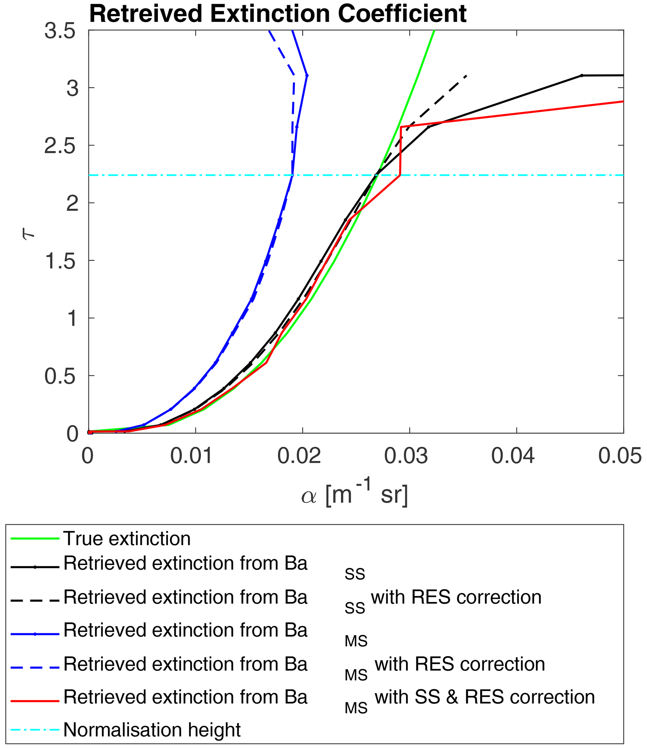
Figure 4Profiles of the retrieved cloud optical extinction retrieved through an inversion of the signal with different corrections. The green line represents the true extinction calculated with the ECSIM. The black solid line represents the extinction profile retrieved without any corrections from the modelled single scattering attenuated backscatter. The dashed black line represents the extinction profile retrieved from the modelled single scattering attenuated backscatter with the resolution correction. The blue solid line represents the extinction profile retrieved without any corrections from the modelled multiple scattering attenuated backscatter. The dashed blue line represents the extinction profile retrieved from the modelled multiple scattering attenuated backscatter with the resolution correction. The red line represents the extinction profile retrieved from the modelled multiple scattering attenuated backscatter with the resolution and multiple scattering correction. The dashed cyan line indicates the beginning of the normalisation interval.
4.1.3 Effects of the range resolution
The finite range resolution of the lidar signal is another factor that influences the final results of the inversion. The range resolution of lidar varies, depending on the system, and the larger it is, the higher its impact might be on the final inversion results. Problems with the resolution of lidar were mentioned before (Evans, 1984) but were never really studied, and no solution to the problem has been proposed so far.
The difficulty associated with the range resolution occurs since practical lidar data are always acquired at a finite resolution and, thus, must be interpreted using a discrete form of solution to the lidar equation. The continuous form of the Eq. (5) is often naively transformed into a discrete form, where the integration is transformed into a summation using, for example, the trapezoid rule, yielding the following:
The above equation is valid for the case where zi<z0; if , then the “+” in the denominator is replaced by a “−”, and the limits of the summation are swapped. Although this is a common practice when transforming continuous equation to discrete form in algorithms, it may not be sufficiently accurate. If the value of α′Δz is small enough, then the approximation by the use of the trapezoid rule is accurate, and the resulting value of α′ corresponds to the bin midpoint. However, if that value is large, the applied approximation is not correct anymore. The detailed explanation of the calculations is presented in Appendix A.
Based on the calculations and using the midpoint of the bins, we define the resolution correction factors (IRES1, IRES2) and RES2 as follows:
and as follows:
where α′(z) is the retrieved cloud optical extinction, and Δz is the height resolution.
IRES2(zi) is applied as a multiplicative correction to the first term within the square bracket within Eq. (11). IRES2(zi) is applied to the last term, while IRES2(zi) is applied as a factor to the numerator and the first term in the denominator.
As the corrections are functions of the extinction itself, in order to apply this correction factor, we need to perform the inversion in two steps. First, we invert the lidar signal and apply the multiple scattering correction. The resulting optical cloud extinction (α) from the first inversion is used in the range resolution correction terms (Eqs. 12–14), and then the corrected signal is inverted again.
Figure 4 presents the retrieved profiles of α with the multiple scattering correction (denoted as MS) and with the multiple scattering correction, together with the range resolution correction (denoted as MS and RES). We observe that, while the MS correction on its own improves the retrieval greatly, after application of the RES correction, values of α are closer to the true value of the extinction coefficient. The importance of the resolution correction can be easily presented when we inverted the simulated single scattering signal (BSS; as mentioned in Sect. 3). Table 2 presents the error and accuracy of the inversion results (as described in Sect. 4.3).
4.2 Estimating cloud base height
Although it is not directly connected to the inversion procedure, an accurate estimation of the cloud base height is also a challenging problem in cloud observation. In this study, we use the peak of the lidar perpendicular signal to evaluate the cloud base height. Lidar power (P(z); Eq. 1) from a depolarisation lidar can be divided into the parallel (P(z)∥) and perpendicular power (P(z)⟂). In every profile we find the peak of the perpendicular power () and estimate the cloud base to be at the height where P(z) is equal to or greater than divided by 10. We found that this estimate predicts the height of cloud base with a good accuracy for the liquid water clouds. Figure 1 presents the radar reflectivity factor and the attenuated backscatter coefficient for the scene used in this study. Both panels present the estimate of the cloud base height marked with a magenta line. Examining the panel with the ATB, we see that our estimate is a good approximation.
4.3 Signal inversion error and accuracy
In this study, we use the ECSIM cloud scene to test the accuracy and estimate the error of the lidar signal inversion. The data set from ECSIM gives us information about the true value of optical extinction coefficient within the cloud. Thanks to that, we can calculate the percent error and the accuracy of the inversion method by comparing the retrieved value to the true (simulated) value of the optical extinction coefficient. For those calculations, we use the following formulas to estimate the percent error:
and the following formulas to estimate the accuracy:
where the subscript BSS is used when we are inverting the signal from the single scattering simulation, and the subscript BMS is used for the simulations from the multiple scattering simulations. For the whole data set, the mean values for each height above the cloud base are presented in Tables 1 and 2 for BSS and BMS, respectively.
Table 1Mean error and accuracy of the cloud optical thickness extinction retrieval for different heights above the cloud base. Data are retrieved by inverting the simulated single scattering signal (BSS) with the estimate calculated from Eq. (7). Results from two inversions are presented, i.e. one without any correction and one with the application of the resolution correction calculated from Eqs. (12)–(14) (noted with the subscript RES).
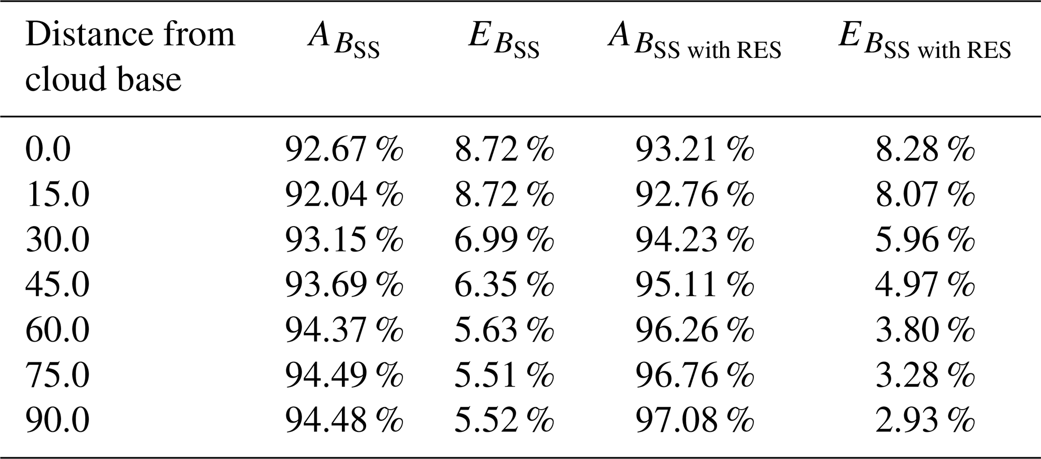
Table 2Mean error and accuracy of the cloud optical thickness extinction retrieval for different heights above the cloud base. Data are retrieved by inverting the simulated multiple scattering signal (BMS) with the α0 estimate calculated from Eq. (7). Results from four inversions are presented, i.e. one without any correction, one with the application of the resolution correction calculated from Eqs. (12) and 14 (denoted with the subscript RES), one with the multiple scattering correction calculated from Eq. (8) (denoted with the subscript MS), and the last one with both the resolution and the multiple scattering correction (denoted with the subscript RES&MS).
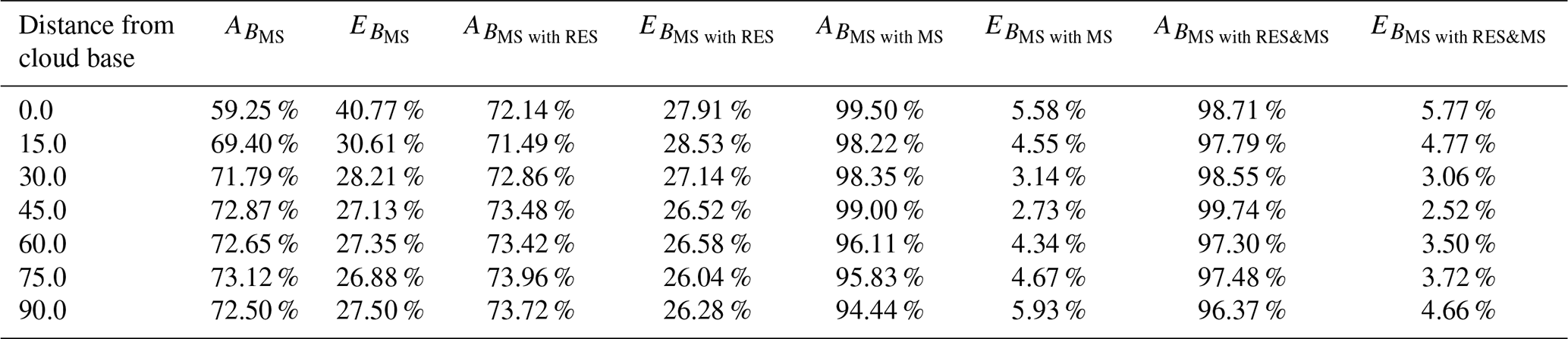
As we indicated before, values retrieved at the cloud base (defined as being 0 m from the cloud base in Tables 1 and 2) are the ones with the biggest percent error. This stems from the difficulty in the signal inversion at very small values of cloud optical extinction. We observe a great improvement in the accuracy of the inversion further within the cloud. We present values of the inversion error and accuracy for the retrieval without any correction and for the retrieval only with the resolution correction ( and ), with the multiple scattering correction ( and ) or with both the multiple scattering and the resolution correction ( and ).
For the results of the inversion of the BSS signal, we tested how the resolution correction can improve the results of the retrieval. Table 1 presents the mean error and accuracy calculated at different levels within the cloud. We observed an increased impact of the resolution correction deeper within the cloud. At a distance of 45 to 90 m from the cloud base, the resolution correction almost doubles the accuracy. This is mostly due to an increase in the value of cloud optical extinction (α). As we explain in the Appendix A, the resolution correction is less relevant for small values of α. Inversion of the signal with the simulated multiple scattering (BMS), and, thus, resembling actual measurements far more, is understandably less accurate. Table 1 presents the mean error and accuracy of the retrieved cloud optical extinction for different heights above the cloud base. Inversion without any correction had a mean error ranging from 40 % at cloud base to 26 % in the cloud. We observed that, with the resolution correction only, the error can be improved by up to 3 %. The correction for the multiple scattering has a much bigger impact; it improves the inversion error by around 35 % at the cloud base and by 20 % higher within the cloud. By combining the resolution and multiple scattering correction, the error of the inversion can be improved to between 6 % at the cloud base and 3 %–4 % within the cloud. We observed that the inversion is most accurate between 30 and 60 m within the cloud. Figure 5 presents the cross section of the retrieval percent error of the cloud optical extinction for the inversion of simulated multiple scattering signal with the inclusion of the resolution and multiple scattering correction. The increase in the error above 60 m from the cloud base is mainly due to an underestimation of the value of the cloud optical extinction at the normalisation height (α0).

Figure 5Cross section of the cloud optical thickness (a) and retrieval percent error of the cloud optical extinction retrieved with the multiple scattering and range resolution correction (b). The magenta line in both panels represents the estimated height of the cloud base, and the black line is the beginning of the normalisation interval.
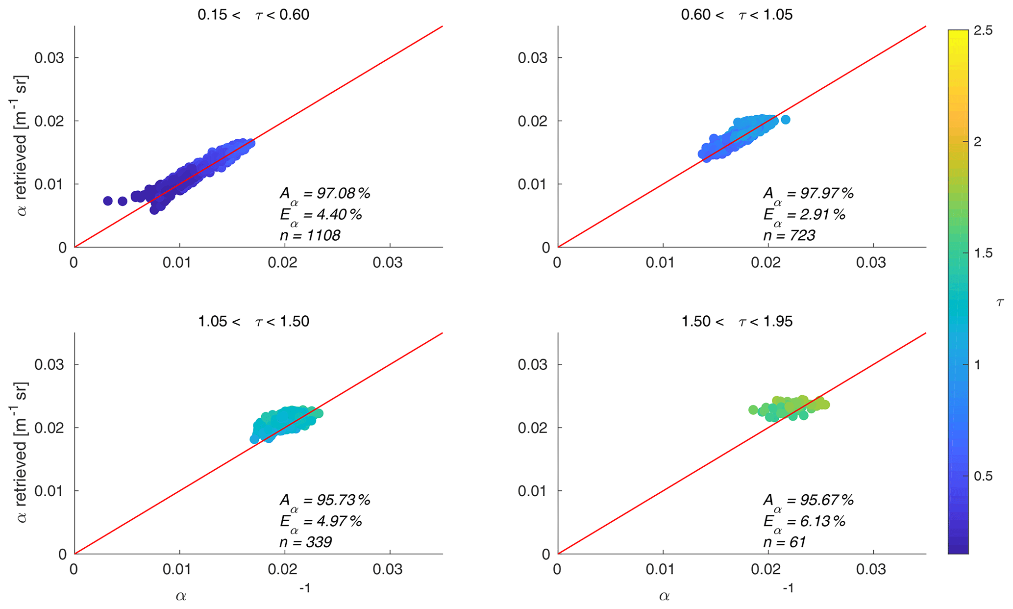
Figure 6Scatterplots of the retrieved cloud optical extinction (with the multiple scattering and range resolution correction) versus the modelled cloud optical extinction from the ECSIM divided into panels depending on the value of the optical thickness. The red line is imposed and represents the equality between the modelled and retrieved values. The colour bar represents the value of the cloud optical thickness at each point. The error Eα (Eq. 15) and accuracy Aα (Eq. 16) for each bin of the optical thickness are also presented.
The accuracy of the retrieval is connected to the cloud optical thickness. Figure 6 presents scatterplots of the retrieved values of α, with the multiple scattering and range resolution correction plotted against the modelled ones. The data are divided by the value of the optical thickness, τ, where, in the following:
α is the cloud optical thickness, and h is cloud depth. Every panel includes an imposed red line which represents an equality between the modelled and retrieved values. We also used a colour scale, where the colour bar represents the value of cloud optical extinction at every point. The error (Eq. 15) and accuracy (Eq. 16) for each bin on the optical thickness are also presented. We observed that the inversion method works best for the values of τ between 0.6 and 1.05. The error for values of τ above 1.5 is higher, and the retrieved cloud optical extinction is underestimated. The probable cause of this behaviour of the retrieval is the loss of a signal with the increase in the cloud optical thickness. For the optical thickness below 0.6 and further below 0.15, the important factor influencing the accuracy of the retrieval is the estimation of the cloud base region.
Figure 5 presents the cross section of the cloud optical thickness and the retrieval percent error. Here, again, we can clearly see that the percent error is highest close to the cloud base, ranging between 8 % and 15 %, and deeper within the cloud it rarely exceeds 7 %. This means that, when inverting the lidar signal, it is important to carefully examine the first range above the cloud base.
4.4 Impact of estimation
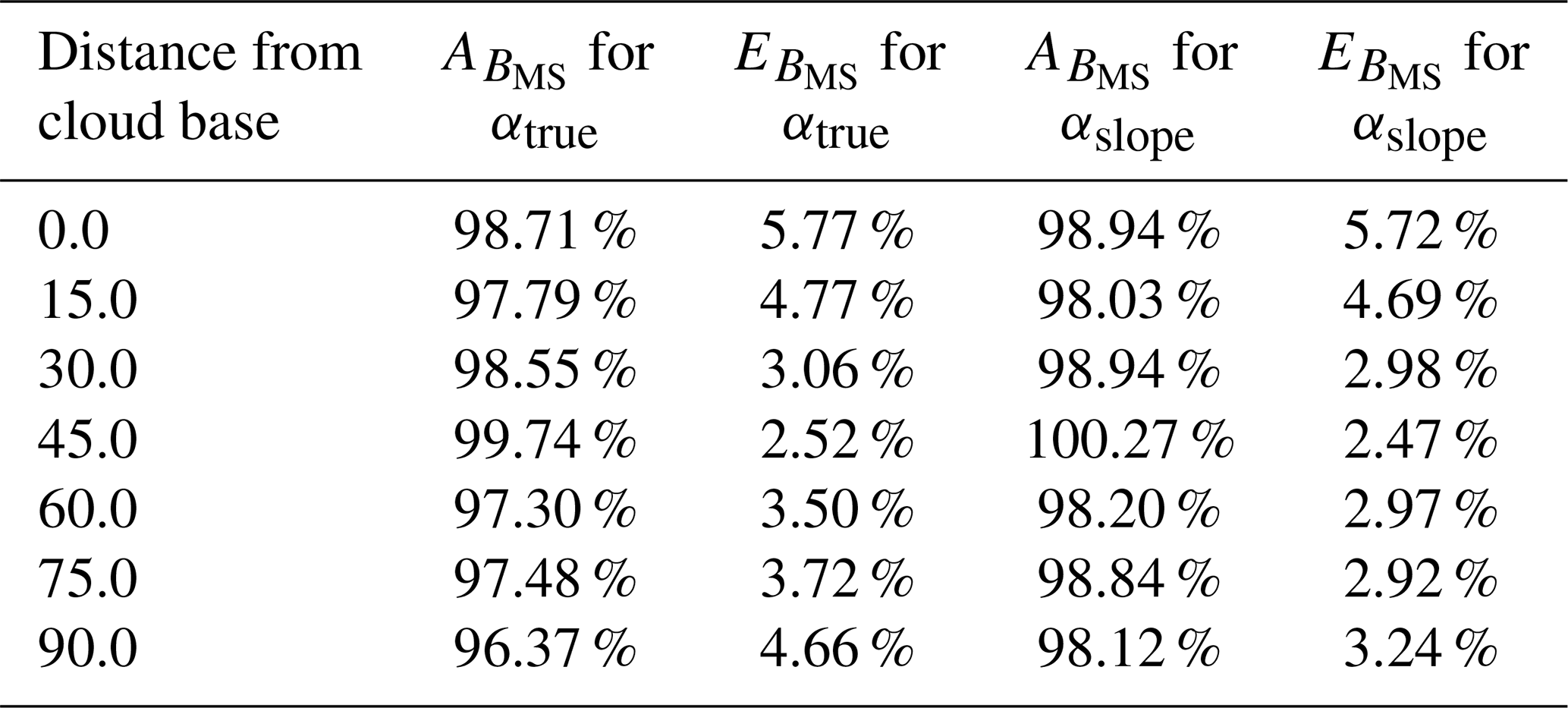
Klett (1981) stated that the value of does not influence the final results of the inversion much. In our study, we tested this statement by performing an inversion with the actual value of extinction at the normalisation height z0 instead of the value calculated from the slope method (Eq. 7). The results of this inversion are presented in Table 3. The error for the inversion with the multiple scattering and resolution correction is improved by around 0.5 %. The error improvement is more significant for the values retrieved above 60 m from the cloud base. This is due to the underestimation of the value of with the slope method (Fig. 2). We also tested the accuracy of the calculated by comparing it to the actual value of α at the normalisation height z0. The mean accuracy of for the whole data set was 95 %, with the minimum accuracy of 89 % and the maximum one of 112 %.
Table 3Mean error and accuracy of the cloud optical thickness extinction retrieval for different heights above the cloud base. Data are retrieved by inverting simulated multiple scattering signal (BMS) with both the resolution and the multiple scattering correction, with α0 equal to the true extinction at the normalisation height z0 (denoted as αtrue) and, in the second case, with the α0 estimate calculated from Eq. (7) (denoted as αslope).
In this paper, we presented a method of lidar signal inversion for the retrieval of the cloud optical extinction in the cloud base region. This method was first presented by Klett (1981). We showed that, with the correction for the multiple scattering within the cloud and the resolution correction, this method can be successfully used for the retrieval of the cloud optical extinction. Both those corrections are essential to improve the accuracy of the retrieved extinction profile and minimise the error. We presented the performance of the retrieval based on the synthetically created cloud scene, where responses of the lidar to specific cloud conditions were simulated. Even though in some cases the cloud base was not varying much in height, the analysed data indicated that the signal inversion close to the cloud base (specifically at the range of the detected cloud base) is prone to error. The retrieval of the cloud optical extinction works better at higher values of the optical thickness. It is, therefore, our recommendation to use only data points located at least one gate range above the detected cloud base height. We also showed that the approximation of calculated with the slope method can be used as an estimation of actual cloud optical extinction at the normalisation height. More importantly, improving the value of by using the actual extinction at the normalisation height does not improve the retrieved values significantly if the correction for the multiple scattering and range resolution is implemented.
We showed that the inversion of the lidar signal with the proposed corrections yields a good estimate of the cloud extinction. Not only is this method fast but can also, because of the use of a standard backscatter depolarisation lidar, be applied to multiple systems and used operationally. Through a link between cloud microphysical properties and the optical extinction, this can provide a valuable data set to be used in the studies of cloud microphysics and impacts of clouds on the climate.
The difficulty associated with the range resolution occurs since practical lidar data are always acquired at a finite resolution and, thus, must be interpreted using a discrete form of the lidar equation. In high-extinction environments, the differences between, for example, the bin mean value and the bin mid values of the range-corrected signal (P(z)z2) can become important and impact the accuracy of applying, for example, Eq. (5) (the specific case relevant to this work). If high accuracy is sought, then the effects of the finite lidar resolution must be accounted for in both the numerator and the second term of the of denominator of Eq. (5).
As a preliminary step, we start by defining the scaled attenuated backscatter as follows:
where Clid is the lidar constant, z is the range from the lidar, P is the measured power, and S is the extinction-to-backscatter ratio. For convenience in this Appendix, we consider the case of a one-component atmosphere. The extension to the two-component case follows trivially by replacing P by P′ and α by α′.
A1 Resolution correction for the integral term
In terms of B(z), an expression analogous to the integral in the denominator of Eq. (5) is as follows:
In discrete form, this becomes the following:
where the zi refers to the bin mid position of the ith range bin, and Δz is the (constant) range bin width. Here, the form is valid for . For the case of , the upper and lower limits of the summation are swapped, and the sign of the whole expression is switched.
With reference to Fig. A1, we can rewrite these expressions in terms of the discrete form of the scaled attenuated backscatter signal for one range gate Bi and the associated half-bin values Bi,1 and Bi,2.
The definitions of the terms in Eq. (A4) can be readily discerned by comparison with Eq. (A3). Equation (A3) indicates that the accurate evaluation of Eq. (A2) involves the summation of the Bi terms and the leading and tailing half-bin terms (the Bi,1 and Bi,2 terms). The Bi terms pose no difficulty as they are directly related to the lidar measurement process in a natural manner (i.e. the lidar (ideally) operates by physically accumulating (in other words, integrating) the return signal between two discrete times corresponding to the range gate boundaries). However, evaluating the edge terms requires more development.
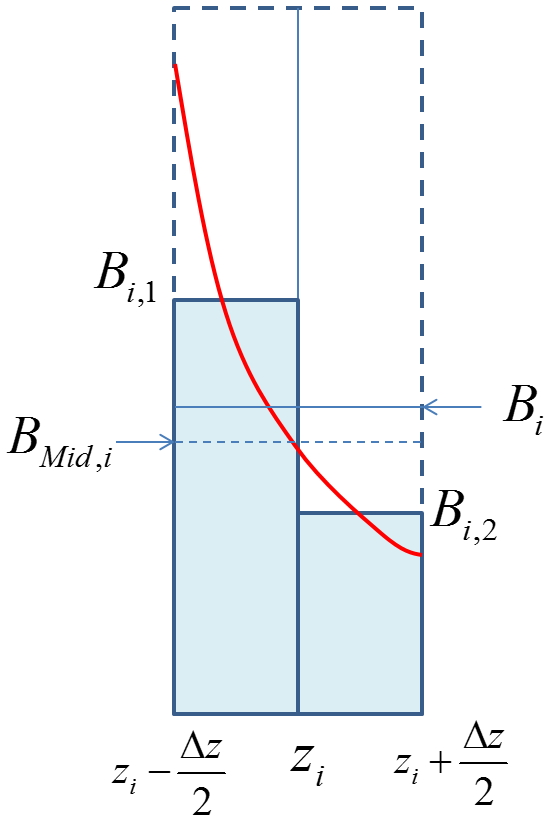
Figure A1Illustration of the relationship between the continuous lidar scaled attenuated backscatter (red line), the bin-integrated average Bi and the half-bin integrated average values (Bi,1, together with Bi,2) and the mid bin value BMid,i.
In order to evaluate the Bi,1 and Bi,2 terms and their relationship with Bi, we start with the single scattering lidar equation in continuous form, which, in terms of B(z), can be written as follows:
where α is the optical extinction. In terms of the optical thickness (τ), Eq. (A5) can be written as follows:
If we assume that α and S are constant within one range gate (this assumption is physically reasonable for fine range resolutions and is also compatible with the lidar model used to generate the simulations used in this work), then using Eq. (A6) Bi can be calculated as follows:
In a similar fashion, B1,i and B2,i are as follows:
and as follows:
If we note that and , then Eqs. (A7)–(A9) lead to the following:
and the following:
Using Eqs. (A10) and (A11), we can now determine the correction terms IRES1 and IRES2 that are applied as multiplicative corrections to the leading and tailing terms, respectively, in the summation representing the integration term in Eq. (11) as follows:
and as follows:
Note that in the optically thin limit, where αΔz tends to zero, IRES1 and IRES2 both tend, as expected, to 1. When αΔz is very large, however, then IRES1 tends towards a limit of 2, and IRES1 tends to 0.
A2 Resolution correction for remaining terms
We now turn our attention to the impact of finite range resolution on the terms not associated with the integral term in Eq. (11). The boundary value of the extinction (e.g. α0) is obviously not impacted; however, the other terms will be affected. In particular, since we are seeking the retrieved extinction values valid at the mid bin point, we must establish the relationship between the bin accumulated signal and the associated mid bin values.
We start by noting that, in terms of B(z) and τ, the single scattering lidar equation (see Eq. A6) can be rewritten as follows:
and the bin mid value (Bm,i) of the ith bin is then just the following:
Equations (A7) and (A15) can then be combined to show that, in the following:
Thus, the desired general form of the correction term (RES2) to be applied to the P′ terms in the numerator of Eq. (11) and the first term of the denominator (but not to the terms under the integral) is as follows:
We note that the term, as expected, tends to 1 for small values of αiΔz.
The algorithm and data used in this publication were published through Zenodo and are available at https://doi.org/10.5281/zenodo.5090535 (Sarna, 2021).
KS developed the software code described in this paper and wrote the paper. DPD contributed to the mathematical derivation of the problem and contributed significantly to the original draft, did the proofreading, and provided guidance throughout the development process. HWJR evaluated and proofread the paper and provided guidance as the supervisor of KS.
The authors declare that they have no conflict of interest.
Publisher’s note: Copernicus Publications remains neutral with regard to jurisdictional claims in published maps and institutional affiliations.
This paper was edited by Edward Nowottnick and reviewed by two anonymous referees.
Albrecht, B. A., Randall, D. A., and Nicholls, S.: Observations of marine stratocumulus clouds during FIRE, B. Am. Meteorol. Soc., 69, 618–626, https://doi.org/10.1175/1520-0477(1988)069<0618:OOMSCD>2.0.CO;2, 1988. a
Cao, X., Roy, G., Roy, N., and Bernier, R.: Comparison of the relationships between lidar integrated backscattered light and accumulated depolarization ratios for linear and circular polarization for water droplets, fog oil, and dust, Appl. Opt., 48, 4130–4141, 2009. a
Carnuth, W. and Reiter, R.: Cloud extinction profile measurements by lidar using Klett’s inversion method, Appl. Opt., 25, 2899, https://doi.org/10.1364/AO.25.002899, 1986. a, b
Collis, R. T. H.: Lidar: A new atmospheric probe, Q. J. Roy. Meteorol. Soc., 92, 220–230, https://doi.org/10.1002/qj.49709239205, 1966. a
Donovan, D. P., Klein Baltink, H., Henzing, J. S., de Roode, S. R., and Siebesma, A. P.: A depolarisation lidar-based method for the determination of liquid-cloud microphysical properties, Atmos. Meas. Tech., 8, 237–266, https://doi.org/10.5194/amt-8-237-2015, 2015. a
Evans, B.: On the Inversion of the Lidar Equation, Tech. rep., Research and Development Branch Department of the National Defence Canada, available at: http://www.dtic.mil/cgi-bin/GetTRDoc?Location=U2&doc=GetTRDoc.pdf&AD=ADA149653 (last access: 7 January 2020), 1984. a
Fernald, F. G.: Analysis of atmospheric lidar observations: some comments, Appl. Opt., 23, 652–653, 1984. a, b, c, d
Fiocco, G. and Smullin, L. D.: Detection of Scattering Layers in the Upper Atmosphere (60–140 km) by Optical Radar, Nature, 199, 1275–1276, https://doi.org/10.1038/1991275a0, 1963. a
Heus, T., van Heerwaarden, C. C., Jonker, H. J. J., Pier Siebesma, A., Axelsen, S., van den Dries, K., Geoffroy, O., Moene, A. F., Pino, D., de Roode, S. R., and Vilà-Guerau de Arellano, J.: Formulation of the Dutch Atmospheric Large-Eddy Simulation (DALES) and overview of its applications, Geosci. Model Dev., 3, 415–444, https://doi.org/10.5194/gmd-3-415-2010, 2010. a
Hu, Y., Liu, Z., Winker, D., Vaughan, M., Noel, V., Bissonnette, L., Roy, G., and McGill, M.: Simple relation between lidar multiple scattering and depolarization for water clouds, Opt. Lett., 31, 1809–1811, https://doi.org/10.1364/OL.31.001809, 2006. a, b, c
Khairoutdinov, M. and Kogan, Y.: A New Cloud Physics Parameterization in a Large-Eddy Simulation Model of Marine Stratocumulus, Mon. Weather Rev., 128, 229–243, https://doi.org/10.1175/1520-0493(2000)128<0229:ANCPPI>2.0.CO;2, 2000. a, b
Klett, J. D.: Stable analytical inversion solution for processing lidar returns., Appl. Opt., 20, 211–220, https://doi.org/10.1364/AO.20.000211, 1981. a, b, c, d, e, f, g, h
Klett, J. D.: Lidar inversion with variable backscatter/extinction ratios, Appl. Opt., 24, 1638, https://doi.org/10.1364/AO.24.001638, 1985. a, b
Kokhanovsky, A.: Optical properties of terrestrial clouds, Earth-Sci. Rev., 64, 189–241, https://doi.org/10.1016/S0012-8252(03)00042-4, 2004. a
McComiskey, A. and Feingold, G.: The scale problem in quantifying aerosol indirect effects, Atmos. Chem. Phys., 12, 1031–1049, https://doi.org/10.5194/acp-12-1031-2012, 2012. a
Müller, D., Wandinger, U., Althausen, D., Mattis, I., and Ansmann, A.: Retrieval of Physical Particle Properties from Lidar Observations of Extinction and Backscatter at Multiple Wavelengths, Appl. Opt., 37, 2260, https://doi.org/10.1364/AO.37.002260, 1998. a
Rocadenbosch, F., Comerón, A., and Pineda, D.: Assessment of Lidar Inversion Errors for Homogeneous Atmospheres, Appl. Opt., 37, 2199, https://doi.org/10.1364/AO.37.002199, 1998. a
Roy, G. and Cao, X.: Inversion of water cloud lidar signals based on accumulated depolarization ratio., Applied optics, 49, 1630–1635, https://doi.org/10.1364/AO.49.001630, 2010. a
Sarna, K.: karrolcia/Klett_lidar_inversion: Klett Lidar Inverison (Version 1), Zenodo [code], https://doi.org/10.5281/zenodo.5090535, 2021. a
Sassen, K. and Petrilla, R. L.: Lidar depolarization from multiple scattering in marine stratus clouds, Appl. Opt., 25, 1450, https://doi.org/10.1364/AO.25.001450, 1986. a
Turner, D. D.: Arctic Mixed-Phase Cloud Properties from AERI Lidar Observations: Algorithm and Results from SHEBA, J. Appl. Meteorol., 44, 427–444, https://doi.org/10.1175/JAM2208.1, 2005. a
Yorks, J. E., Hlavka, D. L., Hart, W. D., and McGill, M. J.: Statistics of Cloud Optical Properties from Airborne Lidar Measurements, J. Atmos. Ocean. Technol., 28, 869–883, https://doi.org/10.1175/2011JTECHA1507.1, 2011. a