Application of cloud particle sensor sondes for estimating the number concentration of cloud water droplets and liquid water content: case studies in the Arctic region

A cloud particle sensor (CPS) sonde is an observing system attached with a radiosonde sensor to observe the vertical structure of cloud properties. The signals obtained from CPS sondes are related to the phase, size, and number of cloud particles. The system offers economic advantages including human resource and simple operation costs compared with aircraft measurements and land-/satellite-based remote sensing. However, the observed information should be appropriately corrected because of several uncertainties. Here we made field experiments in the Arctic region by launching approximately 40 CPS sondes between 2018 and 2020. Using these data sets, a better practical correction method was proposed to exclude unreliable data, estimate the effective cloud water droplet radius, and determine a correction factor for the total cloud particle count. We apply this method to data obtained in October 2019 over the Arctic Ocean and March 2020 at Ny-Ålesund, Svalbard, Norway, to compare with a particle counter aboard a tethered balloon and liquid water content retrieved by a microwave radiometer. The estimated total particle count and liquid water content from the CPS sondes generally agree with those data. Although further development and validation of CPS sondes based on dedicated laboratory experiments would be required, the practical correction approach proposed here would offer better advantages in retrieving quantitative information on the vertical distribution of cloud microphysics under the condition of a lower number concentration.

1 Introduction

Clouds regulate weather and climate systems by radiation, precipitation, and the transfer of heat and moisture (Boucher et al., 2013). They cover a large part of the earth and range in scale from tens to thousands of kilometers (e.g., cyclones or frontal systems). However, the formation process of cloud droplets occurs on the micro-scale through complicated cloud microphysical processes. The simulation of clouds in general circulation models (GCMs) therefore depends on numerous parameterizations.

The composition of clouds involves a liquid phase (including supercooled), a solid phase, or a mixed phase. There are numerous microphysical processes related to the formation of cloud water/ice and falling hydrometeors. In the temperature range between 0 ^∘C and approximately −40 ^∘C, cloud particles may exist both as liquid and ice (Korolev et al., 2017). Although cloud phases and their vertical and horizontal distribution are critical to calculating downward shortwave and longwave radiation, the representation of clouds in climate models, including the partitioning of liquid and ice in clouds, remains a challenging issue because of the poor understanding of cloud microphysical processes.

The partitioning of ice and liquid in mixed-phase clouds controls the radiation budget at the Earth's surface, with particular implications to the vulnerable ice–ocean system of the high latitudes, where the radiative interactions between the microphysical and macrophysical properties of clouds and the surface modify the warming or cooling effect of clouds (Stapf et al., 2020). An overestimation of cloud ice, which has less shortwave radiation reflection, tends to generate a positive sea-surface temperature (SST) bias in the Southern Ocean (Flato et al., 2013). The representation of long-lasting clouds (i.e., cloud water) instead of cloud ice is critical to reducing such SST bias in the Southern Ocean (Varma et al., 2020). Moreover, cloud ice/water fractions in the models represent the air–sea coupled system, which includes ocean circulation and changing winds induced by corrected temperature gradients (Kay et al., 2016).

In the Arctic region, the surface energy budget, particularly over sea ice, is constrained by shortwave radiation during summer and longwave radiation during winter (Intrieri et al., 2002; Persson et al., 2002). The representation of clouds and their impact on radiation fields are therefore vital to simulate future Arctic climate systems. A comparison of regional climate models shows that cloud water is poorly represented in these models (Sedlar et al., 2020). Based on ice-free Arctic Ocean results, Inoue et al. (2021) found that the double-moment cloud microphysics scheme, which solves the mixing ratio and number concentration for each hydrometeor, is superior to the single-moment cloud microphysics scheme. One of the remaining issues is that ice-nucleating particles should be carefully tuned for target seasons/locations when the double-moment cloud physics scheme is applied (Inoue et al., 2021).

Satellites have provided a global perspective of clouds and radiation (Stubenrauch et al., 2013), and satellite data have been intensively used for atmospheric reanalysis (Hersbach et al., 2020). With the advancement of satellite data in recent years as well as computational resources, the presence of global cloud-resolving models (GCRMs), which resolve both large-scale dynamics and small-scale convection, has increased in global weather and climate simulations (Satoh et al., 2019) and global precipitation forecasting with the aid of data assimilation (Kotsuki et al., 2019). Although a general agreement of modeled clouds using satellites in some deep cloud development processes has been reported, GCRMs still depend on cloud microphysical parameterizations, such as high thin cirrus parameters (Kodama et al., 2012).

Despite these advances, the size distribution of cloud particles and vertical distribution of cloud mixing ratios remain poorly validated using observations for boundary layer clouds. Cloud phases can be confirmed by land-/ship-based remote sensing such as long-term monitoring using cloud radars and microwave radiometers (Illingworth et al., 2007; Nomokonova et al., 2019), by a cloud particle imager aboard a tethered balloon system (Lawson et al., 2011), and by a fog monitor at the top of mountain (Koike et al., 2019). For aircraft, great efforts for developing cloud droplet probes have also been made. A bias in the droplet size and/or droplet concentration measured by the cloud droplet probe in flight compared with an independent instrument is attributed to coincidence errors reduced by the improved instrument's optics (Lance et al., 2010). Beswick et al. (2014) succeeded in applying the backscatter cloud probe, which delivers quantitative particle data products including cloud properties, to commercial passenger aircraft as part of the European Union In-Service Aircraft for a Global Observing System program. However, Baumgardner et al. (2017) stated that there remain many outstanding challenges for in situ measurement systems. Unknown particle collection efficiency is a problem for quantitative understanding. The number concentration of clouds is also difficult owing to observation logistics. For example, aircraft observations are costly, which limits the number of feasible flights, and tethered balloons are weather-dependent (i.e., wind speed) and thus limited to a top height of approximately 1000 m. The cost and mobility of observation data are important aspects that should complement existing observation systems, including satellites.

Table 1 Case number of the CPS launch, launch date, ascending speed, horizontal wind speed, air temperature, air pressure, height of cloud layer, air density, cutoff PSW, and effective radius.

^∗ A CPS sonde by the tethered balloon.

A cloud particle sensor sonde (Meisei Electric Co., Ltd.; hereafter, CPS sonde) is an observation system used to obtain the vertical profile of cloud information (e.g., total particle count, particle phases, and particle size) (Figs. 1 and 2). A CPS connected to a normal radiosonde can obtain cloud parameters and basic meteorological profiles. The observation cost consists of the regular launch of a radiosonde and an additional USD 1200 for the CPS. Although theoretical configurations and laboratory experiments have been intensively reported (Fujiwara et al., 2016), the data would require adequate corrections adapted to the individual flight dynamics. The remaining issues are (1) the relationship between flow speed in the CPS inlet and CPS signal; (2) a theoretical understanding of the time interval of each particle signal; (3) characteristics of the aerodynamic flow pattern around the CPS housing, which determines the sampling volume; and (4) validation of the CPS sonde with other observation systems. However, most of these issues are hardly solved by end users who are not always familiar with the detail of the instrument and how to calibrate it by state-of-art techniques. As an alternative way, in this study, we propose a CPS data correction method using the observation data obtained during three Arctic field campaigns (Fig. 1, Table 1) and idealized simulations. The corrected cloud parameters are validated by other observation data sets.

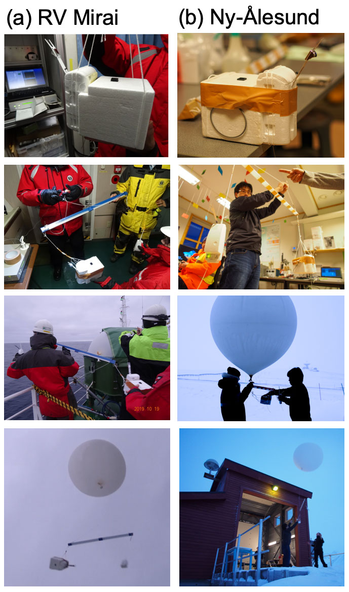
Figure 1 Photographs of the CPS sonde operation at the (a) RV Mirai in October 2019 and (b) Ny-Ålesund in March 2020. The CPS housing within a black inlet duct on top is connected to the Meisei RS-11G radiosonde. During the 2019 and 2020 campaigns, the Vaisala RS41-SGP was attached to the opposite side of the rod.​​​​​​​

Figure 2 Schematic diagram of the CPS (from Fujiwara et al., 2016).

2 Experimental designs

2.1 Field experiments in the Arctic regions

The Arctic research cruise was undertaken by the Japanese ice-strengthened research vessel (RV) Mirai in the Chukchi Sea in November 2018 (Inoue, 2018) (Fig. 3a). This polar night cruise provided favorable conditions for CPS sondes because strong sunlight affects the measurements of scattered light (Fujiwara et al., 2016). The observed area is the marginal ice zone. The total number of observations was 12, of which 6 are used in this study (liquid cloud case). A similar cruise was made in October 2019 (Sato, 2019) (Fig. 3b) in which the observations were made mainly at night. The total number of observations was 12, of which 11 flights are used in this study (Fig. 1a). In addition to the normal CPS sonde observations, the CPS sonde was also applied to onboard tethered balloon observations using an airship-shaped balloon (15 m³, The Weather Balloon Mfg. Co., Ltd.). An instrument bag and a CPS sonde were respectively connected 5 and 10 m below the balloon (Fig. 4). One of the instruments in the bag used in this study was an optical particle counter (OPC; HHPC 6+, Beckman Coulter), which has six channels for particle size ranges of 0.3–0.5, 0.5–1, 1–2, 2–5, 5–10, and > 10 µm with a 10 % coincidence loss. Three channels for sizes > 2 µm were used to validate the total particle counts by the CPS sondes. The ascending speed was typically 0.5–1 m s⁻¹, which strongly differs from the normal CPS sonde observations; however, the impact of ascending speed on particle counting is confirmed by numerical simulation, as discussed later. The maximum height of each flight was lower than 1000 m. Three cloudy cases are investigated in this study.

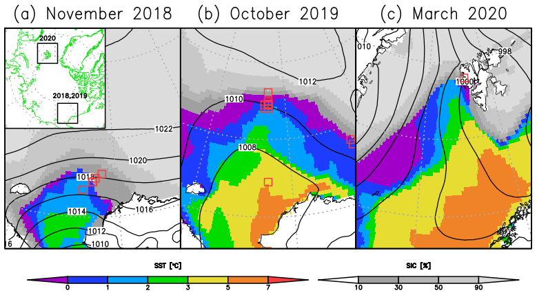
Figure 3 Location of the CPS sondes (red squares) during research cruises in (a) November 2018 and (b) October 2019, as well as (c) a field campaign in March 2020. Monthly mean sea-ice concentration (gray shading), sea-surface temperature (color shading), and sea-level pressure (contours) are based on ERA5 reanalysis.

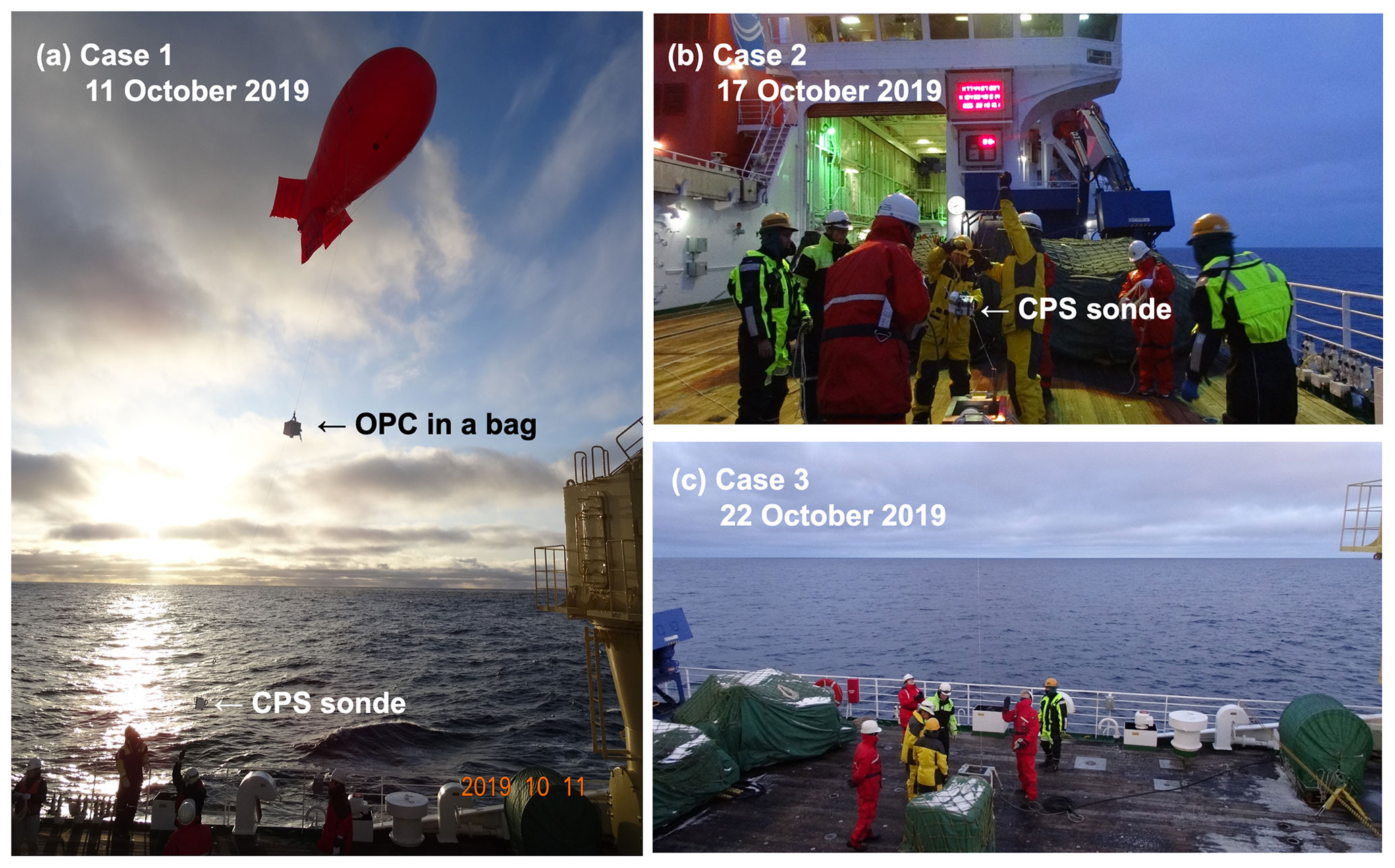
Figure 4 Photographs of tethered balloon measurements for the cases of (a) 11 October 2019 (MR19-CPST1), (b) 17 October 2019 (MR19-CPST2), and (c) 22 October 2019 (MR19-CPST3) on RV Mirai in the Arctic Ocean.

The field campaign based in Ny-Ålesund, Svalbard, Norway, was made in March 2020 (Figs. 1b and 3c). The surface air temperature was approximately −20 ^∘C, which is ∼ 10 ^∘C lower than the previous two cruises. We selected 5 cases out of a total of 14 flights. The liquid water path (LWP) was monitored at the French–German Arctic research base AWIPEV at Ny-Ålesund, Svalbard, which includes the Alfred Wegener Institute (AWI) at the Helmholtz Centre for Polar and Marine Research and the French Polar Institute Paul Emile Victor (IPEV). At the AWIPEV base, a humidity and temperature profiler (HATPRO), a passive microwave radiometer, has been in operation since 2011 (Rose et al., 2005). Nomokonova et al. (2019) reported that more than 90 % of single-layer liquid clouds have LWP values lower than 100 g m⁻². The Cloudnet product (archived at https://cloudnet.fmi.fi/, last access: 13 July 2021) contains an adiabatic retrieval of liquid water content (LWC) when both the cloud radar and lidar detect a liquid layer and microwave radiometer data are present (most reliable classification). In this study, the LWP data and LWC retrieved by the Cloudnet product are used for comparison with the CPS sonde results.

All soundings consisted of a CPS with Meisei radiosondes (RS-11G). The Vaisala radiosonde (RS41-SGP) was also simultaneously launched by hanging from the opposite side of a 1 m long rod in the 2019 and 2020 campaigns (the other side was used for the CPS sonde) (Fig. 1). The balloon type was a 350 g balloon (TOTEX TA350) in the 2018 and 2019 campaigns and a 600 g balloon (TOTEX TA600) in the 2020 campaign. The detailed data list is shown in Table 1.

2.2 Numerical experiments

The simplified three-dimensional computational fluid dynamics (CFD) was simulated using Flowsquare⁺ software (Nora Scientific, https://fsp.norasci.com/en/, last access: 13 July 2021) to better understand the flow pattern around the CPS housing. Flowsquare⁺ solves for density, velocity, temperature, mass fraction of a substance in the fluid, and pressure. The model domain was set to $\mathrm{201}\left(x\right)\times \mathrm{201}\left(y\right)\times \mathrm{601}\left(z\right)$ grids with 1.5 mm in horizontal resolution (Δx=Δy) and 1.0 mm in vertical resolution (Δz). An inflow boundary was specified at the upstream side of the z direction. The remaining boundaries were treated as outflow boundaries under open boundary conditions. The simple 3D object assuming the CPS housing (100 mm × 100 mm × 120 mm) with the Meisei RS-11G radiosonde was used for the inner model boundary condition. The CPS inlet was set to the CPS housing center with 10 mm × 10 mm. Flowsquare⁺ monitors the maximum Courant–Friedrichs–Lewy number and dynamically adjusts the time step size. The air temperature and pressure were set to −20.0 ^∘C and 850 hPa, respectively, assuming the field campaign in March 2020 at Ny-Ålesund. The dynamic viscosity (µ) was fixed at 1.6 × 10⁻⁵ kg m⁻¹ s⁻¹. The ascending speed was set to 5 m s⁻¹ assuming an ascending speed (exp-5m), whereas the horizontal wind speed was fixed to 0 m s⁻¹.

Two types of sensitivity experiments were made: (1) ascending speeds of 4 and 6 m s⁻¹ for typical soundings (exp-4m/6m) and 1 m s⁻¹ for the tethered balloon measurements (exp-1m) and (2) horizontal wind speeds with 2.5 and 5 m s⁻¹ (exp-h2.5m/h5m). In each experiment, a time integration with 4000 steps was made, corresponding to the typical physical timescale of approximately 0.1 s, which is sufficient when the air mass at the initial state passes across the model domain (i.e., quasi-steady state). The list of experiments is shown in Table 2.

Table 2 Experimental CFD setup.

3 Data processing

3.1 Overview of a CPS sonde system and its remaining issues

The technical details of a CPS are described in Fujiwara et al. (2016), from which the essential features are introduced here. A CPS uses a near-infrared laser with a typical 790 nm wavelength as a linearly polarized light source. Two silicon photodiodes are placed at angles of 55^∘ (detector no. 1) and 125^∘ (detector no. 2) to the source light direction (Fig. 2). A polarization plate is placed in front of detector no. 2 so that it only receives light polarized perpendicular to the light source. The two detectors receive scattered light through the slits (0.50 cm × 1.0 cm) in front of them. Fujiwara et al. (2016) determined that the volume of the detection area is estimated as ∼ 1 cm × 1 cm × 0.5 cm, because the two detectors collect light scattered at 55^∘ ± 10^∘ and 125^∘ ± 10^∘. The particle signal voltage from the two detectors (I₅₅ and I_125p) ranges from 0 to 7.5 V with a resolution of 0.03 V. Fujiwara et al. (2016) also defined the particle signal width (hereafter, PSW) which is the particle transit time when I₅₅ first exceeds 0.3 V and the time when I₅₅ falls below 0.3 V.

As described in Fujiwara et al. (2016), owing to the downlink capability of the Meisei radiosondes, only 25 byte s⁻¹ can be transferred to the ground-based receiver. The current CPS provides the following information each second: (i) number of particles (particles s⁻¹), (ii) CPS signal voltage for I₅₅ and I_125p (V) and PSW (ms) for the first six particles entering the instrument each second, and (iii) DC component for the detector no. 1 output. It should therefore be noted that it is impossible to obtain the particle size distribution every second. A statistical and practical approach is necessary to estimate the LWC and LWP.

To distinguish between cloud ice and cloud water, the degree of polarization (DOP) is defined by Fujiwara et al. (2016) as follows.

$$\begin{array}{}\text{(1)}& \mathrm{DOP}={\displaystyle \frac{I_{\mathrm{55}}-I_{\mathrm{125}\mathrm{p}}}{I_{\mathrm{55}}+I_{\mathrm{125}\mathrm{p}}}}\end{array}$$

When the DOP value is negative, the particle is ice (i.e., a non-spherical particle). When the DOP value is positive but less than ∼ 0.3, the particle is most likely ice. When the DOP value is more than ∼ 0.3, the particle is water in many cases (i.e., a spherical particle), but there is a chance that it may be ice because the DOP can take values between −1 and +1 for ice particles. The DOP threshold of 0.3 was originally proposed by Fujiwara et al. (2016) based on laboratory experiments using standard particles; however, they also showed that the DOPs for liquid clouds were usually higher than 0.5 in actual observations (Figs. 4a, 7a, and 10a in Fujiwara et al., 2016). Because the mixed-phase clouds are typical form in the Arctic, the value of 0.5 would be more suitable than 0.3 to reduce the chance of counting ice particles as liquid particles.

3.2 Cutoff PSW to reduce the unrealistic data

According to Fujiwara et al. (2016), a 5 m s⁻¹ flow speed corresponds to a PSW of ∼ 1 ms for a single particle. They also reported that PSW data can be used to monitor potential particle overlap in dense cloud layers. An excessively long signal width may indicate the overlapping of too many particles in the detection area and thus a substantial loss of particle counts. In such cases, multiple light scattering can also occur and complicate the particle measurements.

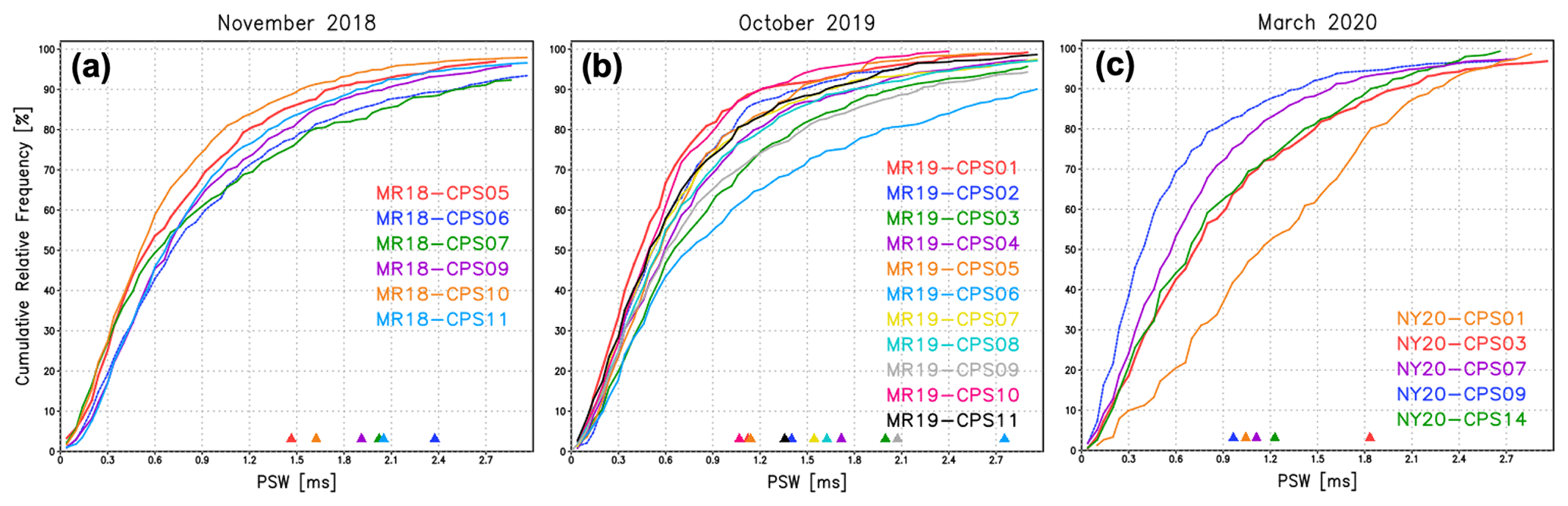
Figure 5 Accumulated relative frequency of PSW for (a) November 2018, (b) October 2019, and (c) March 2020. Each triangle indicates the cutoff PSW (PSW_c).

To confirm the PSW variability, the accumulated relative PSW frequency is plotted for each field campaign in Fig. 5 when cloud water was detected based on a DOP threshold of 0.5. The approximate thickness of the cloud layer for each case is listed in Table 1. Somehow, all the CPS profiles contain PSWs smaller than 1.0 ms with 60 %–80 % relative frequency. We consider the possibility of variable flow speeds in the CPS inlet. Here, we focus on two cases: one with a standard slope curve (NY20-CPS03) and another with a steep slope curve in the smaller PSW range (NY20-CPS09). The mean ascending speeds where liquid clouds were detected was 5.0 and 6.1 m s⁻¹, respectively (Table 1). Faster vertical speed might contribute to the steep slope of the PSW frequency (i.e., smaller PSWs dominate). The difference in the ascending speed therefore has a partial impact on the PSW variability. Furthermore, if the flow speed slows near the inlet wall owing to frictional forces, the PSW might become large because of the time required to pass the detection area (i.e., slower flow speeds require longer times). Considering that more than 50 % of PSW is still smaller than 0.5 ms (i.e., the time to travel the detection zone is short), the detection area might be thinner than 0.5 cm, although the CPS sonde end user hardly verifies the detail (the effect of pulse shapes is discussed in Sect. 5.4.).

The fact that a higher voltage of I₅₅ (i.e., a signal for a larger particle) is observed with the higher PSW (Fig. 6a) suggests that the threshold PSW value can be useful to reduce unrealistic particle size data. This procedure is thus critical to estimate the effective cloud particle radius. Here, the PSW cutoff value (hereafter, PSW_c) is proposed as follows.

$$\begin{array}{}\text{(2)}& \stackrel{\mathrm{‾}}{{\mathrm{PSW}}_{\mathrm{c}}}=\stackrel{\mathrm{‾}}{{\mathrm{PSW}}_{max}-{\mathrm{PSW}}_{min}},\end{array}$$

where PSW_c is the difference between the maximum and minimum PSWs (PSW_max and PSW_min) counted per unit time (=1 s). Note that the number of data is six at most second readings. This procedure thus excludes at least one datum among the six recorded values per second. The overbar indicates the time average where a liquid cloud is observed (typically 50–100 s depending on the cloud-layer thickness). If the PSW is recorded randomly in a detection domain, the ratio of rejected data would be approximately 17 % and the effective data ratio would be approximately 83 %. Using the real cases, $\stackrel{\mathrm{‾}}{{\mathrm{PSW}}_{\mathrm{c}}}$ ranges from 80 % to 90 % (triangles in Fig. 5a–c: except for NY20-CPS01 owing to the thinner sampling depth of 100 m), which supports the randomness of particle counts in the CPS inlet.

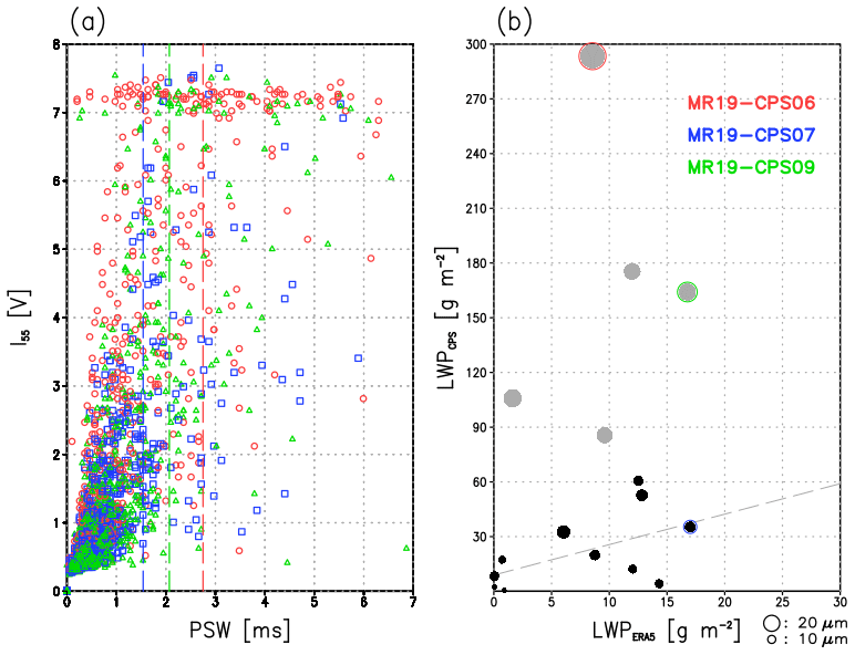
Figure 6 (a) Relationships between PSW (ms) and I₅₅ (V) for MR19-CPS06 (red), MR19-CPS07 (blue), and MR19-CPS09 (green), and (b) scatter plot of LWP (g m⁻²) from ERA5 and CPS sonde for the cruises in 2018 and 2019. Colored dashed lines in panel (a) show the cutoff PSW (PSW_c). Dots in panel (b) indicate the relative size of the mean effective radius (r_e). Gray dots show the cases with r_e larger than 20 µm. A gray dashed line indicates a linear regression line by excluding the cases with r_e larger than 20 µm.

3.3 Estimation of effective particle size

Based on laboratory experiments performed to determine the lower particle size detection limit and relationship between I₅₅ and water droplets, the CPS cannot detect 1 µm diameter polystyrene particles but can detect 2 µm diameter borosilicate glass particles (Table 3) (Fujiwara et al., 2016). The CPS often gives saturated outputs (∼ 7.5 V) for 60 and 100 µm diameter soda-lime glass particles.

Table 3 Laboratory experiments to measure the CPS voltage for various standard particle sizes by Fujiwara et al. (2016).

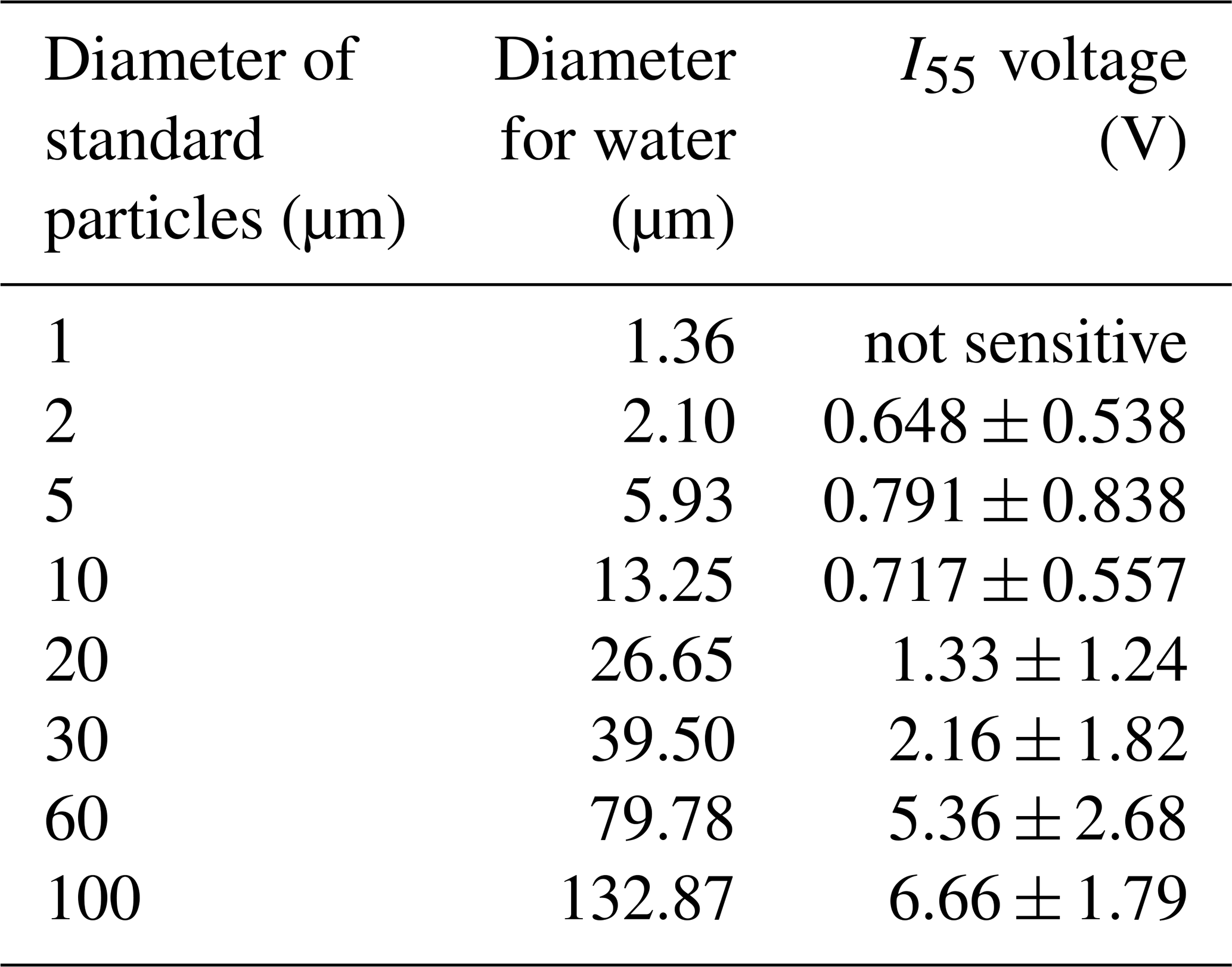
However, they did not provide an empirical equation for estimating particle size, and some approximations are required to estimate LWC and LWP. Although the additional size calibration using optical cloud particle spectrometers might be desired as reported by Lance et al. (2010) and Beswick et al. (2014), it is beyond the scope of this study. In this study, we construct an experimental equation to estimate the liquid cloud effective radius from the measured voltages using the data in Fujiwara et al. (2016). Based on the quadratic regression between log ₁₀(d) and log ₁₀(I₅₅) (correlation coefficient = 0.983, p value: 7.28 × 10⁻⁵), the following empirical equation is proposed:

$$\begin{array}{}\text{(3)}& {\log }_{\mathrm{10}}\left(d\right)=\sqrt{{\displaystyle \frac{{\log }_{\mathrm{10}}\left(I_{\mathrm{55}}\right)+\mathrm{0.13303}}{\mathrm{0.4257}}}}+\mathrm{0.09831},\end{array}$$

where d is the diameter that corresponds to the observed voltage (I₅₅) of a particle. Considering that the number of I₅₅ data is 6 s⁻¹ at most and one of which will be excluded where PSW_max is larger than PSW_c, only five data sets are available to estimate the particles sizes. Although random sampling is assumed, as discussed in Sect. 3.2, time averaging in a certain thickness would better represent the section of cloud layers. Here, the averaging time is set to ±2 s, corresponding to a 25 m thick cloud layer. The effective radius (r_e: µm) of the cloud droplets is estimated by considering volume averaging as follows:

$$\begin{array}{}\text{(4)}& r_{\mathrm{e}}={\displaystyle \frac{{\left({\sum }_{k=\mathrm{1}}^n{d}_n^{\mathrm{3}}\right)}^{\mathrm{1}/\mathrm{3}}}{\mathrm{2}n}},\end{array}$$

where n is the number of observations in the target cloud layer (typically 5 particles s⁻¹ × 5 s = 25 particles) and d_n is the nth particle diameter estimated by Eq. (3).

3.4 Correction factor of total particle count

Once the r_e is determined at each level, the LWC and LWP can be estimated if the total particle count is correct. Fujiwara et al. (2016) roughly estimated that the CPS can correctly measure number concentrations up to ∼ 1000 particles s⁻¹ under a flow speed (v) of 5 m s⁻¹. In the case of dense clouds, the PSW might be larger than 1 ms owing to signal overlap and thus lose particle counts. Fujiwara et al. (2016) therefore proposed a correction factor (f) for the total count of particles per second as $f=\mathrm{4}\times (\mathrm{PSW}/(\mathrm{5}/v){)}^{\mathrm{3}}$ if the PSW, which is the maximum among up to six values per second, is greater than $\mathrm{5}/v$; if the PSW is smaller than $\mathrm{5}/v$, f=1. The corrected count N_cor (s⁻¹) can thus be estimated using f and the original count N_org (s⁻¹) as follows.

$$\begin{array}{}\text{(5)}& N_{\mathrm{cor}}=f\times N_{\mathrm{org}}\end{array}$$

However, this assumption is only be applicable if a 5 m s⁻¹ flow speed corresponds to a PSW of ∼ 1 ms for a single particle. Considering that the PSW varies widely (Fig. 6a) and most PSWs are smaller than 1.0 ms with 70 % of the accumulative relative frequency (Fig. 5), the sampling overlap (PSW > 1.0 ms) might be a minor factor.

Here we consider the shape of the CPS housing with a radiosonde. The flow at the top of the housing during ascent (assuming 5 m s⁻¹) would be modified and aerodynamically slowed (< 5 m s⁻¹). This reduced inflow into the CPS inlet leads to a loss of cloud particle counts. Fujiwara et al. (2016) measured the flow speed at the bottom of the inlet (i.e., the bottom side of the CPS housing) by using hot-wire anemometers. The flow speed at the bottom side was around 4.7 m s⁻¹ below 5 km height, which was about 15 % smaller than the balloon ascending rate (around 5.5 m s⁻¹) (Fig. B1 in Fujiwara et al., 2016). This means that the downstream flow is heavily modified by the CPS cube-shaped housing, thus causing a large pressure drag with turbulent wakes near the CPS housing's bottom side. The CPS housing's background flow should therefore be carefully considered to correct the cloud particle count.

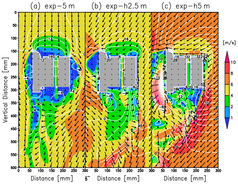
We calculated the flow pattern around the CPS housing using Flowsquare⁺. Figure 7 shows the flow pattern assuming an ascending speed of 4, 5, and 6 m s⁻¹. The flow speed in the CPS inlet increases with increasing ascending speed. Compared with the three cases, the pressure gradient between the top and bottom sides (i.e., pressure drag) regulates the flow speed in the CPS inlet (white contours in Fig. 7). The flow speed at the bottom side for each case (3.4 m s⁻¹ in exp-4m; 4.3 m s⁻¹ in exp-5m; 5.2 m s⁻¹ in exp-6m) is about 15 % smaller than the ascending speed, which is the similar result to Fujiwara et al. (2016). This supports that our simulation is valid for further investigation of flow characteristics around the CPS housing.

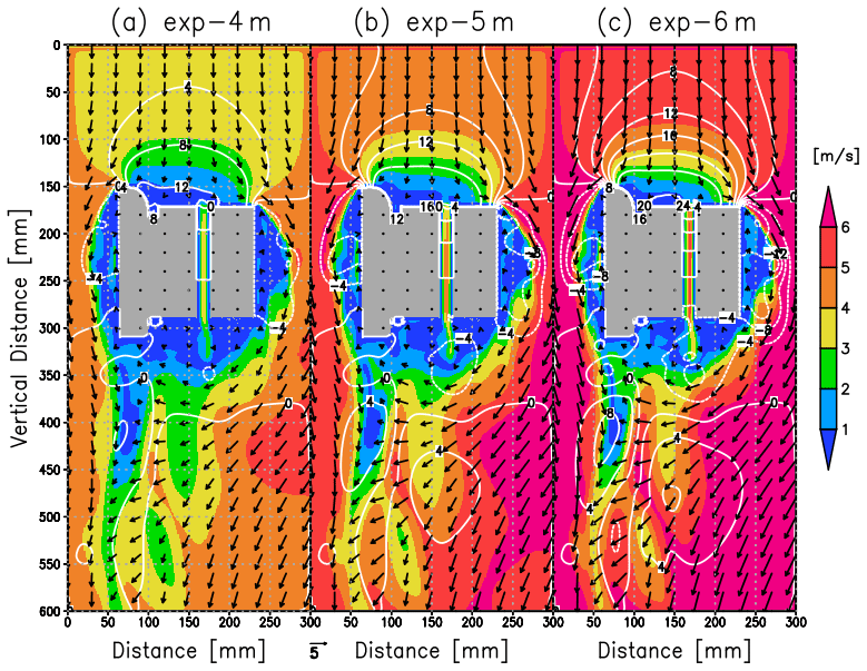
Figure 7 Cross section of the simulated flow speed around the CPS housing (absolute speed: m s⁻¹) assuming an ascending speed of (a) 4 m s⁻¹, (b) 5 m s⁻¹, and (c) 6 m s⁻¹. Contours and gray shades indicate the pressure difference from the initial state (Pa) and CPS housing.

Noll and Pilat (1970) introduced the total collection efficiency (E) and local collection efficiency (B) on a rectangle body as expressed by $E=\mathrm{2}{y}_{\mathrm{0}}^{\ast }/L$ and $B=\mathrm{\Delta }{y}_{\mathrm{0}}/\mathrm{\Delta }{y}_{\mathrm{s}}$, where $y_{\mathrm{0}}^{\ast }$ is one of trajectories of y₀ originated from ambient upstream point and tangent to the body, y_s is the ordinate at the body surface for a certain y₀, and L is the width of the body. Under a hyperbolic flow regime, B becomes uniform across the body surface (Noll and Pilat, 1970), suggesting B=E. In our case, once E is obtained, B over the CPS inlet can be indirectly obtained. Here, we estimate E by calculating the trajectories of $y_{\mathrm{0}}^{\ast }$ using the result of exp-5m (Fig. 8). In the x direction, the innermost trajectories are not symmetric because of the shape of an attached radiosonde (Fig. 8a), while in the y direction, the two trajectories are symmetric (Fig. 8b). Considering that most of these trajectories are on the hyperbolic airstream (black contours in Fig. 8), the number concentration of particles would be reduced near the top of the CPS housing, in particular for smaller size particles. Using the initial distance between two trajectories in each direction as $\mathrm{2}{y}_{\mathrm{0}}^{\ast }$ and the width of the CPS housing as L, each component of E is obtained as E_X=0.284 and E_Y=0.079, and then $E=\sqrt{E_X\times E_Y}=\mathrm{0.148}$. This value might vary with particle size and ascending speed; however, the averaged state is assumed in this study (the need for laboratory experiments will be discussed later). By averaging the results by different ascending speeds (1, 4, 5, and 6 m⁻¹), the mean B is estimated as 13.3 ± 1.8 %. The correction factor for total particle counts (f) is therefore proposed as 7.5 ($=\mathrm{1}/\mathrm{0.133}$).

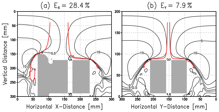
Figure 8 Innermost trajectories against the CPS housing (indicated by red lines) for the (a) horizontal x direction (u component) and (b) horizontal y direction (v component). E_X and E_Y indicate the estimated collection efficiency (%) for each component. Black lines are absolute constants of hyperbolic flow.

4 Comparison with other data sources

4.1 Total particle count by a tethered balloon in the Arctic Ocean

The OPC’s vertical profiles on the tethered balloon are used to evaluate the corrected total particle count by the CPS sonde. The OPC’s count is based on a 5 s suction (L⁻¹), whereas the CPS’s count is based on a 1 s interval. Thus, the CPS count is averaged by 5 s. The data in which the DOP values are larger than 0.5 are used for comparison, focusing on the liquid cloud. The CPS count unit (s⁻¹) is standardized to that of the OPC (L⁻¹) by the ascending speed at each level (typically ∼ 1 m s⁻¹) and the cross section of the detection area of the CPS inlet (1 cm²).

Figure 9 shows the vertical distribution of the number concentration of particles larger than 2 µm obtained by the OPC and CPS sonde. A 50 m thick cloud layer characterizes case 1 at 400 m height where the OPC detected a peak value of around 10 000 L⁻¹, whereas the CPS significantly underestimates this value. This discrepancy arises from the low cloud cover of the thin stratus clouds (Fig. 4a), introducing horizontal and vertical heterogeneity in the measurements because of the vertical distance between both systems of 5 m with a slight tilting. Sunlight (Fig. 4a) might affect the count of the signal (the DOP values lower than 0.5 under high air temperature do not indicate ice cloud particles' existence). Nevertheless, the top and bottom of the cloud are consistent with values of approximately 2000–3000 L⁻¹. The second case is the thickest cloud case among the three (Fig. 4b). The observation terminates at 750 m height, but the moist layer (relative humidity > 95 %) continues until approximately 1200 m, as confirmed by a regular-time Vaisala RS-41 radiosonde observation (not shown). A cloud bottom height of 600 m with 97 % relative humidity matches well where the number concentration starts to increase. The rapid increase in concentration where the relative humidity is 100 % is also very similar. Although both sensors detect a lower number concentration up to 700 m height, the remarkable difference between the two occurs at heights between 700 and 750 m. The OPC value continuously decreases, whereas the CPS value rapidly increases. This discrepancy arises from the detectable range of the sensors because the CPS has a wider particle size range, which suggests that larger cloud particles dominate at this level. The averaged I₅₅ voltage at 600–650 and 700–750 m corrected by $\stackrel{\mathrm{‾}}{{\mathrm{PSW}}_{\mathrm{c}}}$ is 0.61 and 1.27 V, respectively, which corresponds to ∼ 2 and ∼ 25 µm in diameter (Table 3). The former particles are detected by the OPC, whereas the latter are likely out of range. The third case is the intermediate case in terms of the cloud layer (120 m thick) (Fig. 4c). The two concentration peaks at heights of 690 and 730 m are well matched. The third peak in the CPS sonde at 760 m height is characterized by the larger particles out of the OPC range.

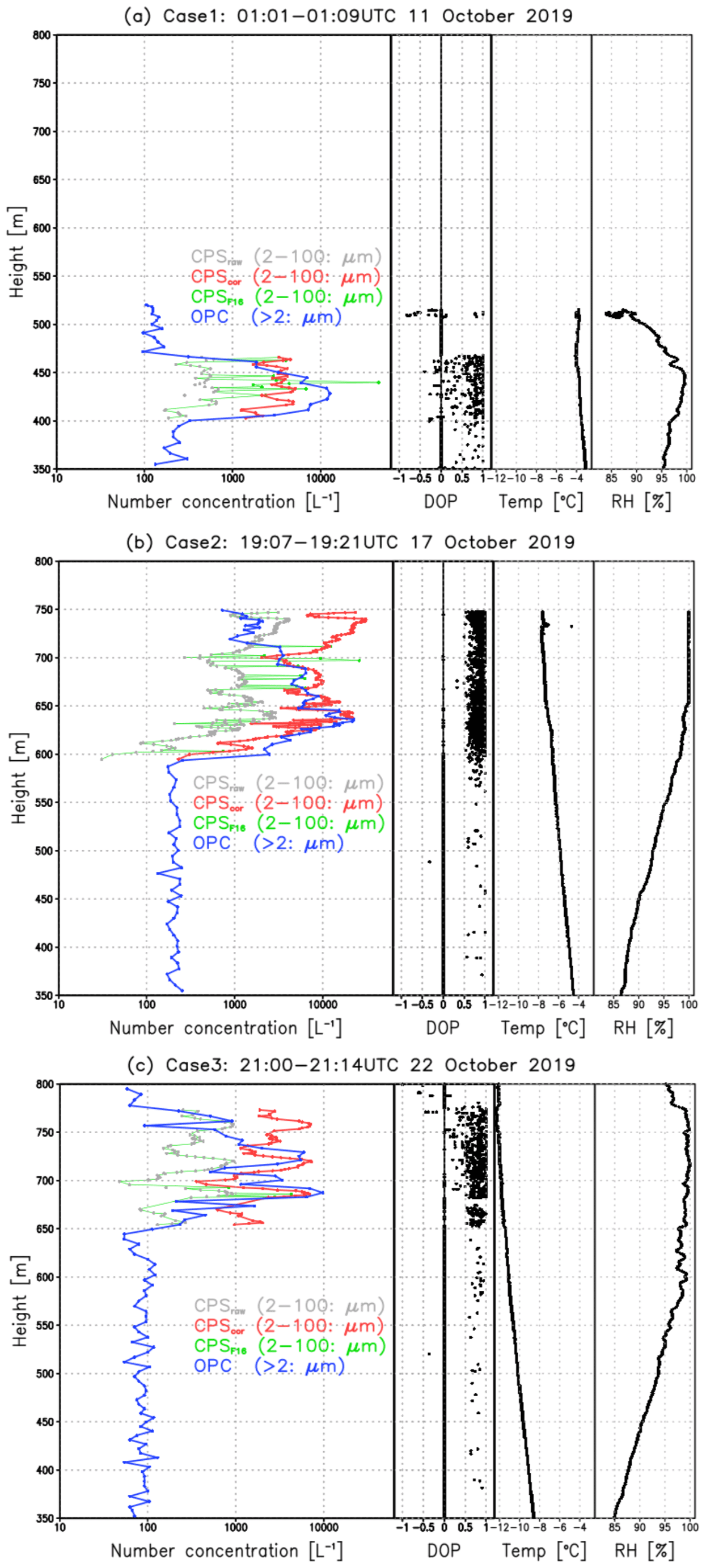
Figure 9 Vertical distribution of the number concentration of particles larger than 2 µm by the OPC (blue) and CPS sonde (corrected in this study in red; corrected by Fujiwara et al., 2016, in green) during the tethered balloon measurements on RV Mirai. Gray dots indicate the original CPS total counts. The values of DOP, air temperature, and relative humidity are indicated by black dots and black lines for each case.

The total particle count corrected by the factor proposed by Fujiwara et al. (2016) is nearly the same as the raw particle count, leading to a significant underestimation (green line in Fig. 9). Because the slow ascending speed promotes $\mathrm{5}/v$ larger than the PSW, the factor is frequently unity (i.e., 1.0) by the definition of Fujiwara’s factor. Despite the difference in the detectable particle size range and sampling method (suction vs. natural ventilation by the ascending motion) between the OPC and CPS sonde, the correction factor for the CPS’s total particle count proposed in this study offers a promising advantage to provide meaningful physical information for the quantitative analysis of cloud microphysics processes.

4.2 LWC and LWP by microwave radiometry at Ny-Ålesund, Svalbard

Using the land-based remote sensing product at Ny-Ålesund, r_e and PSW_c are applied to estimate and validate LWC and LWP. The Cloudnet product is only available for a portion of the March 2020 data set to retrieve the LWC. Only the NY20-CPS03 case is available for comparison. Because this case is the single-layer cloud case (400 m water cloud depth) and the LWP from the Cloudnet product is 30.4 g kg⁻¹ at 17:10 UTC on the measurement day, which is larger than the typical uncertainty of the HATPRO (20–25 g m⁻²), comparison with the CPS sonde is feasible.

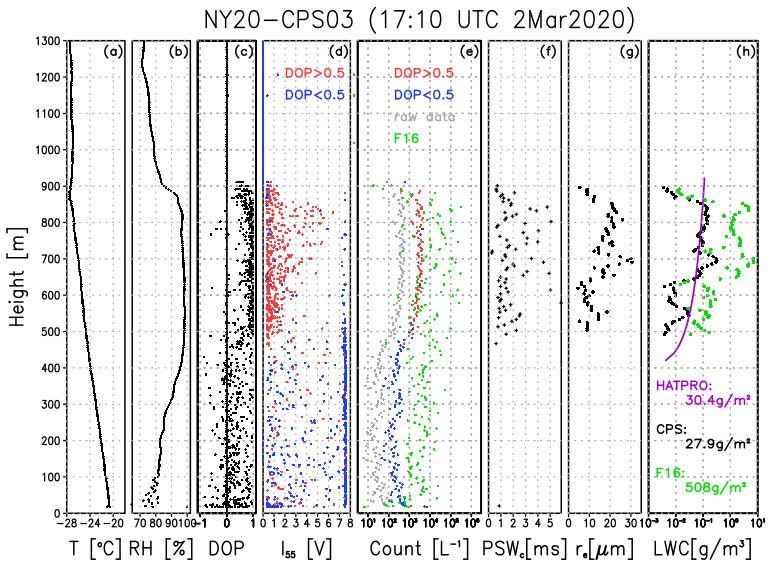
Figure 10 Vertical distributions of (a) air temperature (^∘C), (b) relative humidity (%), (c) DOP, (d) I₅₅ (V), (e) total particle count (L⁻¹), (f) PSW_c (s⁻¹), (g) effective liquid particle radius, and (h) liquid water content (g m⁻³). The numbers in panel (h) indicate the amount of the liquid water path (g m⁻²) calculated by each method.

To estimate LWC, r_e is calculated at each level by satisfying the PSW_c threshold value to Eqs. (3) and (4). The LWC can be estimated assuming the cloud droplet shape is a sphere and water density is 1000 kg m⁻³. Figure 10 shows the vertical profiles of air temperature, relative humidity, I₅₅ voltage, DOP value, total particle count, PSW_c, r_e, and LWC. This case is characterized by mixed-phase clouds where the lower layer up to 500 m is filled by cloud ice or snow (i.e., the DOP value is small; blue dots in Fig. 10), whereas the upper layer from 500 to 900 m is dominated by cloud water (e.g., the DOP is larger than 0.5; red dots in Fig. 10).

Based on the vertical distribution of the I₅₅ voltage, r_e increases from ∼ 10 to 25 µm with two peaks at 700 and 830 m. PSW_c ranges between 1 and 5. The I₅₅ voltage sometimes exceeds 7 V, which suggests that PSW_c appropriately reduces the samples larger than the CPS detection limit or solid cloud phase. The LWC increases up to 850 m with a maximum of 0.25 g m⁻³. This peak value does not depend on the total particle count but rather the size of r_e. These characteristics generally agree with the adiabatically retrieved LWC by the Cloudnet product, which linearly increased up to the cloud top. The vertical integration of LWC, namely LWP, shows that the CPS sondes (27.9 g m⁻²) tend to underestimate the LWP by the Cloudnet (30.4 g m⁻²). A possible reason might be cloud ice contamination. The DOP threshold between cloud ice and cloud water is set to 0.5 in this study. If a more strict DOP threshold is applied, the LWP increases (e.g., to 36.1 g m⁻² for a DOP threshold of 0.7); however, the number of samples for the r_e calculation decreases with considerably higher uncertainty of the LWC calculation. It should also be noted that the LWP data from the Cloudnet product also have a given uncertainty, as previously mentioned before. In other words, the LWP value by the CPS sonde falls within the range of the Cloudnet product uncertainty.

If the correction factor by Fujiwara et al. (2016) is applied to this case, the total particle count (∼ 10⁴ L⁻¹: green dots in Fig. 10) is 1 order larger than our corrected value (∼ 10³ L⁻¹) and thus overestimates LWP (506 g m⁻²). Although the true r_e is unknown, a combination of corrected total particle count and r_e using PSW_c can provide new insight into understanding the vertical structure of liquid phase clouds.

5 Discussion

5.1 Limitation for estimating LWP by CPS sondes

Because ERA5 (Hersbach et al., 2020) can qualitatively simulate liquid-phase clouds in the lower troposphere over the ice-free ocean (Inoue et al., 2021), a comparison of CPS-derived LWP (LWP_CPS) with ERA5 (LWP_ERA5) can provide additional insight on the estimation of LWP_CPS, in particular how unrealistic an obtained value may be. A comparison with the hourly ERA5 outputs at the closest grid point of the ship is made in the case of the Arctic cruises from 2018 and 2019 to avoid topographic effects at Ny-Ålesund in ERA5. Figure 6b shows a scatter plot between LWP_ERA5 and LWP_CPS. Several outliers show a common feature: a mean r_e larger than 20 µm (gray dots). By excluding these five cases, the correlation coefficient between LPW_ERA5 and LWP_CPS is 0.55, with a p value of 0.082. LWP_CPS is almost twice as much as LWP_ERA5 because ERA5 uses a coarser vertical resolution (seven layers below 850 hPa). The cloud microphysics without solving each hydrometeor number concentration would be the other factor. Of course, several error sources can arise from the corrected CPS sonde data. In any case, abnormal LWP_CPS values would occur in the case of relatively large particle sizes, which are larger in I₅₅.

The MR19-CPS06 case (largest r_e case: 31 µm) reveals that the voltage in I₅₅ frequently reaches the maximum regardless of the degree of PSW (red circles in Fig. 6a), whereas the MR19-CPS07 case (normal r_e case: 14 µm) does not exhibit such a condition (blue squares in Fig. 6a). The former case has a larger PSW_c of 2.75 ms (red dashed line Fig. 6a), which cannot correctly exclude the saturated voltage data and thus causes unrealistic r_e and LWP_CPS. The latter case successfully leaves the data via PSW_c (blue dashed line in Fig. 6a). In the intermediate PSW_c case with 2.07 ms, the number of saturated I₅₅ voltage is reduced (MR19-CPS09: green dashed line in Fig. 6a); however, the LWP_CPS is still 10 times larger than LWP_ERA5 with r_e=22 µm. Extra caution is therefore needed for high PSW_c (e.g., > 2.0 ms).

5.2 Other sources to modify the collection efficiency

The simulations show that the flow speed in the CPS inlet becomes fast with increasing ascending speed (v) (Fig. 7), leading to a decrease in $\stackrel{\mathrm{‾}}{{\mathrm{PSW}}_{\mathrm{c}}}$. The correlation coefficient between v and $\stackrel{\mathrm{‾}}{{\mathrm{PSW}}_{\mathrm{c}}}$ is −0.58 (p value: 0.0023) if the tethered balloon cases are included. The pressure height (p) is another factor to modify $\stackrel{\mathrm{‾}}{{\mathrm{PSW}}_{\mathrm{c}}}$ (correlation coefficient = 0.57, p value: 0.0027). The multiple linear regression correlation coefficient to predict $\stackrel{\mathrm{‾}}{{\mathrm{PSW}}_{\mathrm{c}}}$ with v and p is 0.71 with an F value of 0.0003. Therefore, both v and p are important environmental parameters for determining $\stackrel{\mathrm{‾}}{{\mathrm{PSW}}_{\mathrm{c}}}$. Fujiwara et al. (2016) monitored the CPS inlet flow speed by attaching a duct with anemometers at the bottom of the CPS inlet (Fig. B1 in Fujiwara et al., 2016) and showed that the difference between them increases with increasing height, particularly in the stratosphere.

Although half of the variability of $\stackrel{\mathrm{‾}}{{\mathrm{PSW}}_{\mathrm{c}}}$ can be explained by v and p, the remainder may be related to other potential factors, including (1) tilting of the CPS housing induced by horizontal winds, (2) rotation of the CPS housing, and (3) swing between the CPS sonde and balloon (20 m distance). These effects might change the local collection efficiency B and the flow speed in the inlet. Because the pressure gradient between the top and bottom sides of the CPS housing controls the CPS inlet flow speed (Fig. 7), the impact of horizontal wind speed on the pressure fields should be verified. Additional simulations were thus performed assuming horizontal winds (v_h) of 2.5 and 5 m s⁻¹ (Table 2) under the v of 5 m s⁻¹ to understand how the wind angle against the CPS housing modifies the pressure field. As expected, the pressure and flow patterns differ substantially from the experiments without horizontal wind (Fig. 11). In exp-h5m, the flow speed in the CPS inlet decreases compared with exp-5m even if the ascending speed is the same because the large pressure gradient is present at both lateral sides of the CPS housing rather than the top–bottom sides. This decreased flow speed in the inlet would cause a larger PSW. Under actual conditions, the CPS housing would be tilted by horizontal winds with rotation and swing, which complicates the relationships between horizontal wind speed and CPS inlet flow speed. B would be also changed due to the distortion of the asymmetric distribution of hyperbolic flow.

Figure 11 Same as Fig. 7 but for different horizontal wind speeds: (a) 0 m s⁻¹, (b) 2.5 m s⁻¹, and (c) 5 m s⁻¹.

5.3 Necessity of additional laboratory experiments

So far, the cloud microphysics probes for a research aircraft have been developed eagerly by focusing on many aspects (e.g., theoretical optical configurations, specialized simulations, dedicated calibrations using known size particles). Lance et al. (2010) found that calibrations by water droplets of known size were not consistent with theoretical instrument response with a 2 µm shift in the manufacturer's calibration compared with calibrations with polystyrene latex and glass beads. They argued that a misalignment of the optics relative to the laser beam axis caused this discrepancy. In our study, the size calibration relies on the data from Fujiwara et al. (2016) by using standard particles. In addition to this, the shape of the CPS laser beam is not uniform although it is adjusted to be relatively uniform with a biconvex lens (Takuji Sugitachi​​​​​​​, Meisei Electric Co., Ltd., personal communication, 2021​​​​​​​). The detecting domain's heterogeneity could be measured by the calibration system with water droplets of known size by a piezoelectric droplet generator device as Lance et al. (2010) and Beswick et al. (2014) did, contributing to the accurate estimation of finer size distribution by the CPS sonde. Although the CPS calibration is out of the scope of CPS sonde users' skills, continuous developments and collaborations have to be necessary between the manufacturer and users.

Ideally, the concentrations of particles entering the inlet are the same as that in the free stream (i.e., isokinetic sampling); however, the sample velocity is often much smaller than the ambient velocity as shown by Fujiwara et al. (2016) and our simulations (i.e., sampling is sub-isokinetic). The reduction of sample velocity is the issue of aspiration efficiency defined as the ratio of particle concentrations at the inlet entrance to that in the free stream (Craig et al., 2013). The local collection efficiency (B) estimated in this study might be related to particles' concentrations at the inlet entrance and depends on the particle size (i.e., B increases as particles size increases) because I₅₅ is sometimes saturated even under the lower PSW (< 1 ms) situation (e.g., red marks in Fig. 6a). Regarding the impact of the particle size on the collection efficiency, Murakami and Matsuo (1990) evaluated it by using a hydrometeor videosonde system (HYVIS: Meisei Electric Co., Ltd.) which has two small TV cameras to take pictures of hydrometeors from 7 µm to 2 cm from the 25 mm × 50 mm inlet. They found that the collection efficiency increases from 10 % to 50 % as the particle diameter increases without airspeed dependency partly because a larger particle has a higher inertial force in the penetrating air. Although this is the HYVIS case, the development of a housing with a streamlined shape to reduce significant air resistance at the top of the CPS sonde and the estimation of B by laboratory experiments would be desired.

5.4 Limitation of CPS sondes

Regarding the large variations in PSW, we assumed that the differences between the observed PSW (PSW_o) and the expected one (PSW_e) are mainly caused by variations in the CPS housing flow dynamics. Here, we discuss the possibility of non-uniform beam intensity and non-uniform beam effect on modifying the pulse shape and resultant PSW_o. Although the shape of the CPS laser beam is adjusted to be relatively uniform with a biconvex lens, the PSW_o is potentially decreased from PSW_e if the pulse shape is not rectangular but another shape caused by the heterogeneity of the laser beam. Here, we assess the relationship between I₅₅ and PSW_o, assuming that the pulse shape is a sine curve. By definition, PSW_o is recorded in the case of I₅₅ > 0.3 V. Therefore, the PSW_o holds the following relationship as a function of I₅₅; $I_{\mathrm{55}}/\mathrm{2}\times \sin \left(\mathrm{2}\mathit{\pi }\right({\mathrm{PSW}}_{\mathrm{o}}/{\mathrm{PSW}}_{\mathrm{e}}+\mathrm{0.25})+\mathrm{1})=\mathrm{0.3}$. An ideal case (PSW_e = 1.0) is considered here. The relationship between I₅₅ and PSW_o derived using this equation is shown in Fig. 12a (a black line). In the case of lower I₅₅, the smaller PSW_o is expected because of the smoothed shape of the pulse. This situation is significant when I₅₅ is smaller than 1.0 V. The data observed in the Arctic regions are mostly on the black line, suggesting that the CPS counted the particles as a single particle in the case of the smaller pulse intensity (I₅₅ < 3 V). This assessment is also consistent with the cumulative relative frequency of PSW shown in Fig. 5. For the larger pulse intensity (I₅₅ > 3 V), the overlapping would occur but was not significant for our data (Arctic regions).

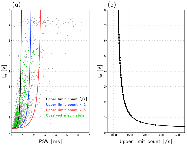
Figure 12 (a) Estimated relationship between PSW and I₅₅ based on the upper limit of countable particle number (a black line) in the case of PSW_e = 1.0. Blue and red lines indicate the doubled and tripled situations from the normal upper limit count. Gray dots are the same plot in Fig. 6a. Green dots indicate the mean state for each second after applying the cutoff value of PSW (PSW_c). (b) Upper limit of countable particle number as a function of I₅₅ in case of PSW_e = 1.0.

Figure 13 Flow chart for calculating LWP from the raw CPS data.

The shorter PSW_o for smaller particles allows us to count the more particles in a unit time (e.g., 1 ms). For example, a particle with I₅₅ = 0.5 V takes 0.33 ms; thus, three particles can be counted in 1.0 ms. In contrast, a larger particle with 5.0 V takes 0.84 ms. Therefore, the relationship (a black line in 12a) can be converted to the upper limit for the countable particle number in a unit time (per second) as shown in Fig. 12b. If the background number concentration is very low (e.g., 1000 particles s⁻¹), then every size can be detected as a single particle. In case that the concentration is relatively high (e.g., > 2000 s⁻¹), however, particle overlap is potentially expected for the larger particles. In such a situation, the value of PSW_o (blue and red lines in Fig. 12a) can be considered an overlap factor for particle overlap. Because this factor would depend on the background number concentration, the users should determine the value by checking the PSW-I₅₅ relationship. In our case, the background number concentration is low (typically < 1500 particles⁻¹), and the majority of the observed particles have relatively small sizes; thus, the effect of the overlap factor (around 1.5 or less) on estimating the total count is relatively small compared with the effect of collection factor (= 7.5). However, the estimated r_e and LWC might be underestimated because the count for larger particles might be underestimated (PSW > 2 ms). In fact, the amount of LWC in Fig. 10h from the CPS sonde was lower than that from HATPRO. In any case, this discussion is based on the assumption that the pulse shape is a sine curve; therefore, we do not conclude the exact value of the overlap factor; nevertheless, the observed relationship between I₅₅ and PSW would be a valuable indicator to confirm the size range in which the CPS sonde measures the clouds correctly for each launch.

In our observations, the typically observed counts were around 2000 L⁻¹, which corresponds to 1000 particles s⁻¹. Because the phase detection depends on the first six particles per second (i.e., 0.6 % of 1000 particles), the representation of size distribution in every second might be insufficient. However, the fact that the corrected number concentration matched with the OPC measurements reveals that the correction method in this study would be applicable for the clouds under relatively low number concentration without particle overlapping. The reason would be related to the collection efficiency of the CPS housing. Considering the collection efficiency of 13.3 % derived from Sect. 3.4, the number of expected particles that pass across the CPS inlet would be 133 particles s⁻¹. Considering that it usually takes tens of seconds to observe a few hundred-meter-thick clouds, it should be noted that each of the first six particles during the assent are not selectively counted. Assuming the mean state of the clouds in five seconds (i.e., a 25 m thick cloud layer), 30 particles are available for estimating the size and phase of particles (more than 20 % of expected particles). This condition represents the total size distribution under a 90 % significant level with 10 % permissible error. Of course, one should pay attention to the clouds when high number concentrations and larger particles are expected. In mixed-phase clouds, the liquid phase droplets might predominate due to smaller particles, introducing the biased DOP value toward the droplets rather than ice. Choice of the DOP threshold between ice and liquid is also challenging (in this study, 0.5 was proposed as the DOP threshold). Overall, the instantaneous value obtained by the CPS sonde does not represent the cloud characteristics at the level sufficiently, in particular under relatively higher number concentration with larger droplets; however, the situation under relatively lower number concentration with smaller droplets allows the CPS sondes to measure the mean state of the clouds.

6 Conclusions

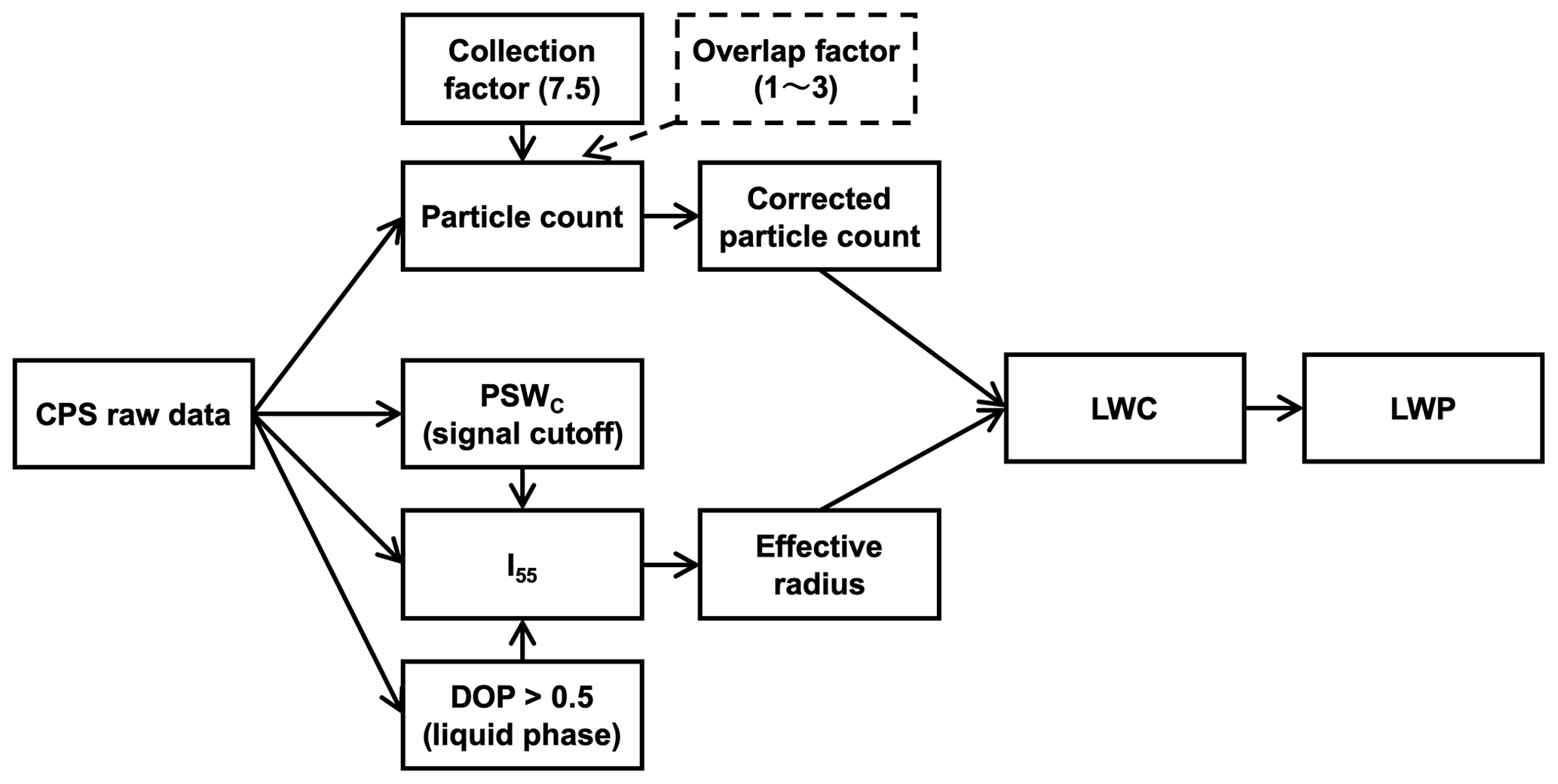
The CPS sonde is a unique observation system to measure cloud phases and total particle counts and sizes; however, this system requires appropriate flight-adapted corrections to obtain quantitative and meaningful results. Figure 13 summarizes the procedure to calculate LWP using the raw CPS data. In this study, a collection factor of 7.5 for total particle count correction is proposed that considers the particle collection efficiency at the top of CPS housing. Although the overlap correction factor, which has initially proposed by Fujiwara et al. (2016) under typical ascending speeds (5 m s⁻¹), was also discussed and might range between 1 and 3, the factor was not incorporated in this study partly because of the smaller background number concentration in the polar regions. A direct comparison with the OPC on tethered balloon measurements shows that this proposed correction factor can estimate the total particle count. The discrepancy between CPS sonde and OPC data occurs at the level where larger particles dominate (e.g., > 10 µm), which is out of the OPC range.

In this study, we focus on a liquid-phase cloud in the first trial. To estimate LWC and LWP, an empirical formula to calculate the effective radius r_e from the I₅₅ voltage is proposed based on laboratory experiments by Fujiwara et al. (2016). However, the I₅₅ voltage sometimes contains outliers close to the maximum CPS voltage limit. In such cases, the PSW value, which is the time interval of each particle signal, also increases (Fig. 6a). The PSW has previously been considered as a constant (1.0) if the flow speed is 5 m s⁻¹; however, nearly 70 % of PSWs are usually smaller than 1.0 ms, as shown in Fig. 5. Although there are only six samples of PSW per second, we propose a cutoff value of PSW (PSW_c), defined as the difference between the maximum and minimum PSW. The PSW_c is not a constant but varies in each launch and second because PSW depends on the flow speed (ascending speed and possibly horizontal wind speed) and ambient air pressure. Although the validation is only in one case, the LWC and LWP estimated by the CPS sonde broadly capture the characteristics obtained by land-based remote sensing.

This study focused on the Arctic region from fall to spring, which favorably reduced the effects of sunlight for the CPS sonde observations. However, additional nighttime field experiments at lower latitudes, at which the amount of moisture and clouds are larger than in the polar region, would advance data evaluation from CPS sondes. From the CPS users' side, the continuous development of the CPS sonde system by the manufacturer (e.g., optical setting, the shape of housing) through additional laboratory experiments and theoretical interpretation is strongly desired.