Cloud height measurement by a network of all-sky imagers

Cloud base height (CBH) is an important parameter for many applications such as aviation, climatology or solar irradiance nowcasting (forecasting for the next seconds to hours ahead). The latter application is of increasing importance for the operation of distribution grids and photovoltaic power plants, energy storage systems and flexible consumers.

To nowcast solar irradiance, systems based on all-sky imagers (ASIs), cameras monitoring the entire sky dome above their point of installation, have been demonstrated. Accurate knowledge of the CBH is required to nowcast the spatial distribution of solar irradiance around the ASI's location at a resolution down to 5 m. To measure the CBH, two ASIs located at a distance of usually less than 6 km can be combined into an ASI pair. However, the accuracy of such systems is limited. We present and validate a method to measure the CBH using a network of ASIs to enhance accuracy. To the best of our knowledge, this is the first method to measure the CBH with a network of ASIs which is demonstrated experimentally.

In this study, the deviations of 42 ASI pairs are studied in comparison to a ceilometer and are characterized by camera distance. The ASI pairs are formed from seven ASIs and feature camera distances of 0.8…5.7 km. Each of the 21 tuples of two ASIs formed from seven ASIs yields two independent ASI pairs as the ASI used as the main and auxiliary camera, respectively, is swapped. Deviations found are compiled into conditional probabilities that tell how probable it is to receive a certain reading of the CBH from an ASI pair given that the true CBH takes on some specific value. Based on such statistical knowledge, in the inference, the likeliest actual CBH is estimated from the readings of all 42 ASI pairs.

Based on the validation results, ASI pairs with a small camera distance (especially if <1.2 km) are accurate for low clouds (CBH<4 km). In contrast, ASI pairs with a camera distance of more than 3 km provide smaller deviations for greater CBH. No ASI pair provides the most accurate measurements under all conditions. The presented network of ASIs at different distances proves that, under all cloud conditions, the measurements of the CBH are more accurate than using a single ASI pair.

1 Introduction

Cloud base height (CBH) has become an important parameter in meteorology that is required, either directly or indirectly, in many applications. The CBH is used to validate and improve climate models (Costa-Surós et al., 2013) and numeric weather prediction models (Hogan et al., 2009). In aviation, CBH is important to air traffic controllers (Khlopenkov et al., 2019; Reynolds et al., 2012; Isaac et al., 2014). As clouds are the major cause of the variability in the solar resource, they are of special interest for solar power applications. Here, the CBH is of interest to forecast the solar resource for the next seconds to hours ahead (nowcasting). All-sky imager (ASI)-based nowcast methods require cloud top height (CTH) and CBH to calculate the position and extent of cloud shadows on the ground (Nguyen and Kleissl, 2014). In a similar way, satellite-based nowcast methods can profit from accurate knowledge of the CBH and CTH (Bieliński, 2020). The statistical relationship between the CBH and a cloud's further properties, like optical thickness, can be exploited to support the generation of such nowcasts (Nouri et al., 2019c). Also, cloud tracking schemes, used in ASI-based nowcasting, require knowledge of the CBH to estimate the absolute displacement of clouds over time.

The method for measuring the CBH, presented in this study, is used as part of an ASI-based nowcasting system of the solar resource. ASI-based nowcasting is typically applied if variations in irradiance have to be predicted for lead times immediately ahead (0…20 min) and at the highest temporal and spatial resolution (e.g., 30 s and 5 m, respectively, as used by Nouri et al., 2020b). Such nowcasts can reduce the uncertainty of supply from solar power plants and can support the efficient balancing of energy supply and demand (Law et al., 2014; Kaur et al., 2016). Furthermore, they can be applied to control concentrating solar power plants (Nouri et al., 2020a) more efficiently. The coordination of renewable production and energy consumption at a local scale is a way to minimize the requirements from grid infrastructure while keeping the curtailment of feed-ins from renewable sources at a low level. Ghosh et al. (2016) use nowcasts (15 s ahead) to control photovoltaic (PV) feed-in and provide reactive power. In this context, spatially and temporally highly resolved nowcasts enable distribution grid operators, microgrid controllers and energy management administrators to control backup power, energy storage and flexible consumers. Cirés et al. (2019) pointed out the potential of nowcasts to reduce the battery storage capacities required by PV plants under ramp rate restrictions. As implied above, high quality and real-time information of the local CBH is required at all sites for which accurate nowcasts should be provided.

CBH, required in ASI-based nowcasting, can be estimated in multiple ways. Most commonly, CBH is measured by ceilometers or other lidars. In Germany, the meteorological service Deutscher Wetterdienst (DWD) operates a network of ceilometers that has a distance between stations of approximately 60 km in the region of the measurement site at Oldenburg (Chan et al., 2018). Ceilometers are specialized instruments that come at a high price and provide the CBH zenith-wise for the location of their installation. Therefore, we do not consider ceilometers as an option to provide the CBH in real time for most solar power plants or cities with many rooftop installations. Further common approaches to measuring the CBH, which could be applied for operational use in nowcasting, include weather balloons and the estimation of the CBH based on a recognized cloud genus (World Meteorological Organization, 2018). Satellites can measure the CTH of the highest cloud layer (Hamann et al., 2014) but require estimations of cloud vertical extent (see, e.g., Noh et al., 2017) to provide the CBH. ASIs can directly measure the CBH but require estimations of the cloud vertical extent if CTH is of interest. In ASI-based nowcasting, the double use of ASIs for the estimation of the CBH besides cloud recognition is considered advantageous in a trade-off between system costs and accuracy.

The ASI-based estimation of the CBH may follow different principles. Some approaches first measure the angular velocity of clouds in the sky image of a single ASI and estimate the CBH with an external source of cloud velocity. Wang et al. (2016) derives cloud velocity by three photocells placed at known distances from each other. Kuhn et al. (2018b) measures cloud velocity by a cloud speed sensor based on nine photocells and by a shadow camera system and compares the accuracy of the received CBH. Tomographic reconstruction approaches (Mejia et al., 2018) or, similarly, voxel carving approaches (Nouri et al., 2018) first model 3-D representations of clouds from which their base height can be retrieved.

Stereoscopic approaches match features found in the images of two ASIs. Used ASIs are located in proximity to each other and, in this way, form an ASI pair. From the position of matched features in both images, the CBH is triangulated. The literature describes various image features which can be utilized for this task. Blanc et al. (2017) exploits gradients of intensity. Allmen and Kegelmeyer Jr. (1996) used local velocity in an image point derived by optical flow. Similarly, Savoy et al. (2016) utilized a 3-D scene flow by making use of the slow evolution of cloud structures. Kuhn et al. (2018b) subtract red channel images taken with a temporal offset of 30 s and match the image areas with the most significant changes. Features from the images of both cameras are typically matched by a block-wise cross-correlation, while the used block size may vary between the approaches. Beekmans et al. (2016) generated dense 3-D representations of cumulus clouds using semi-global block-matching with a very fine block size of 11×11 pixels. Image areas, for which features are retrieved, are often restricted to areas that are segmented as clouds in a prior step (e.g., Blanc et al., 2017; Peng et al., 2015). The stereoscopic approach utilized here (Nouri et al., 2019a) enhances the approach by Kuhn et al. (2018b) and works completely independently from cloud recognition which is considered to bring a greater robustness. While stereoscopic and voxel carving or tomographic approaches are, in principle, competing techniques, Nouri et al. (2019a) demonstrated that voxel-carving-based cloud modeling can be enhanced by incorporating the CBH from a stereoscopic procedure.

Most ASI-based nowcasting systems described in the literature feature one (Schmidt et al., 2016), two (Allmen and Kegelmeyer Jr., 1996; Beekmans et al., 2016; Blanc et al., 2017; Savoy et al., 2016) or three (Peng et al., 2015) ASIs. In total, four ASIs have been used by (Kuhn et al., 2018a; Nouri et al., 2019a), and such systems are available at four different sites (Nouri et al., 2020b). A network of six ASIs accompanied the HD(CP)² Observational Prototype Experiment (HOPE) measurement campaign in 2013 around Jülich, Germany (Macke et al., 2017). In the city state of Singapore, a larger number of 16 ASIs, interacting in a network to monitor the sky and clouds (in the following referred to as ASI network), has been set up (Sky cameras, 2020). A method for monitoring clouds with an ASI network using tomographic reconstruction has been described conceptually and has been based on synthetic data by Mejia et al. (2018). Aides et al. (2020) studied a similar approach experimentally using an actual ASI network of up to 14 cameras located in an area of 12 km × 12 km around Haifa, Israel. ASI networks have additionally been reported as having been used in astronomy to track meteorites during nighttime (Howie et al., 2017).

In this study, seven of the ASIs included in the Eye2Sky ASI network (Schmidt et al., 2019; Blum et al., 2019a, b) are used. The selected ASIs are located in the city of Oldenburg. At the time of writing, Eye2Sky contains 24 ASIs in Oldenburg and in a region of about 110 km × 100 km to the west of Oldenburg. Eye2Sky is mainly dedicated to nowcasting of solar irradiance at a high spatial and temporal resolution. The forecasting procedure, which will be described in more detail in a future publication, first recognizes clouds from the images of the ASIs. Cloud observations are then projected into a horizontal plane at the current CBH. These georeferenced cloud observations of multiple ASIs are merged and cloud properties are estimated. The angular velocities of clouds, as recognized by the individual ASIs, are transformed into absolute velocities over ground relying on an accurate estimation of the CBH. Clouds are tracked along received cloud motion vectors to predict the clouds' future positions. Prior works studying ASI-based forecasting systems with up to four cameras (e.g., Nouri et al., 2019b) suggested that the CBH is an essential component when predicting maps of solar irradiance based on cloud observations from ASIs, as the current and future positions of cloud shadows on the ground can only be predicted accurately if the clouds' height and velocity are determined accurately. Thus, in this publication, an important component of this nowcasting system, namely the estimation of the CBH, is presented. Our approach allows one to use multiple ASI pairs organized as an ASI network, and located in proximity to each other, to estimate the CBH. A total of 42 ASI pairs are formed from the seven ASIs, and the CBH is estimated by each ASI pair based on the method presented by Nouri et al. (2019a). In a period of 3 months, the accuracy of the included ASI pairs is evaluated for distinct conditions. Gained knowledge about the deviations of each ASI pair is applied to merge the measurements of the CBH from all 42 ASI pairs into a more reliable measurement.

This publication is structured as follows. First, Eye2Sky, the ASI network used in the experiments, is introduced (Sect. 2). Then, the measurement procedure of the CBH using the ASI network is presented (Sect. 3). Here, the properties of the CBH measured by reference ceilometer and by 42 ASI pairs are discussed (Sect. 3.1). The meteorological conditions at the site are studied next (Sect. 3.2). In Sect. 3.4 and 3.3, a novel procedure to combine the CBH measurements from multiple ASI pairs of the ASI network is presented. Section 4 analyzes the CBH measurement by the ASI network in comparison to the individual ASI pairs for all relevant conditions. A summary of the presented findings closes the study in Sect. 5.

2 Eye2Sky network and experimental setup

The so-called Eye2Sky ASI network is being set up in the region of Oldenburg (Fig. 1; left). At its full extent, Eye2Sky will include 38 stations distributed over an area of roughly 110 km× 100 km, each of which will be equipped with an ASI. In total, 13 of these stations will be supported by additional meteorological measurements to provide beam, diffuse and global irradiance via rotating shadowband irradiometers, as well as ambient temperature and relative humidity. A total of eight ceilometers will be included in the network. Of these, six are operated by the meteorological service Deutscher Wetterdienst (DWD), and five of these ceilometers are in the region shown in Fig. 1. Several PV plants and numerous smaller distributed PV installations are also present in the study area. With its regional coverage, Eye2Sky aims to achieve nowcasts for individual PV installations from some minutes to multiple hours ahead. In the urban area of Oldenburg, the network will feature a high density of 14 ASIs in an area of 13 km × 12 km. This dense setup aims to provide ASI-based nowcasts of high accuracy across the urban area, and a reliable estimation of the CBH under all conditions is an important contribution to achieve this scope.

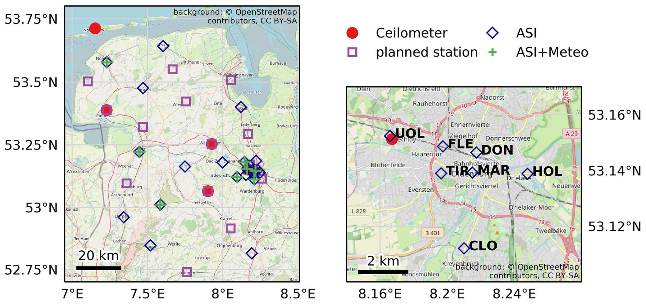
Figure 1 Overview of the Eye2Sky ASI network including operational ASIs (ASI), radiometric measurements (Meteo) and planned stations (left) and ASIs in the city of Oldenburg that have been included in this study (right). The ceilometer used as a reference (marked by a red circle in the right figure) is located near the northwestern-most ASI UOL. Background source: © OpenStreetMap contributors, 2021. Distributed under the Open Data Commons Open Database License (ODbL) v1.0.

This work utilizes seven ASIs (labeled UOL, FLE, DON, TIR, MAR, HOL, and CLO) and one ceilometer located in the city of Oldenburg (Fig. 1; right). The ceilometer is located 133 m southeast of to the northwestern-most ASI UOL (University of Oldenburg; see Fig. 1 on the right) . All included ASIs, except for UOL, are located east and south of the ceilometer. ASIs are placed, at most, 5.7 km from this ceilometer.

For this study, these ASIs are arranged into several ASI pairs as defined by iteratively selecting a tuple of two ASIs out of the 21 tuples available and forming two independent ASI pairs from each tuple by swapping its main camera. The main camera of an ASI pair is central to the measurement of the CBH through an ASI pair, described in more detail in Sect. 3.1, and defines the center of the area for which the CBH is estimated. From 21 tuples of 2 ASIs, 42 ASI pairs are received. All 42 ASI pairs are included in the estimation procedure. The distance of the paired cameras and the orientation of the axis of the ASI pair characterize the ASI pairs. The orientation of an ASI pair's axis is defined as seen from the main ASI and is given in degrees north. Figure 2 shows the distribution of orientations of ASI pairs' axes (left) and camera distances (right) in the set of available ASI pairs. This set covers almost all possible orientations of ASI pairs' axes. Available camera distances 0.8…5.7 km cover most of the range 0.02…5.5 km that is used in the literature (Kuhn et al., 2019). Only towards small camera distances below 0.8 km does the present set lack further ASI pairs.

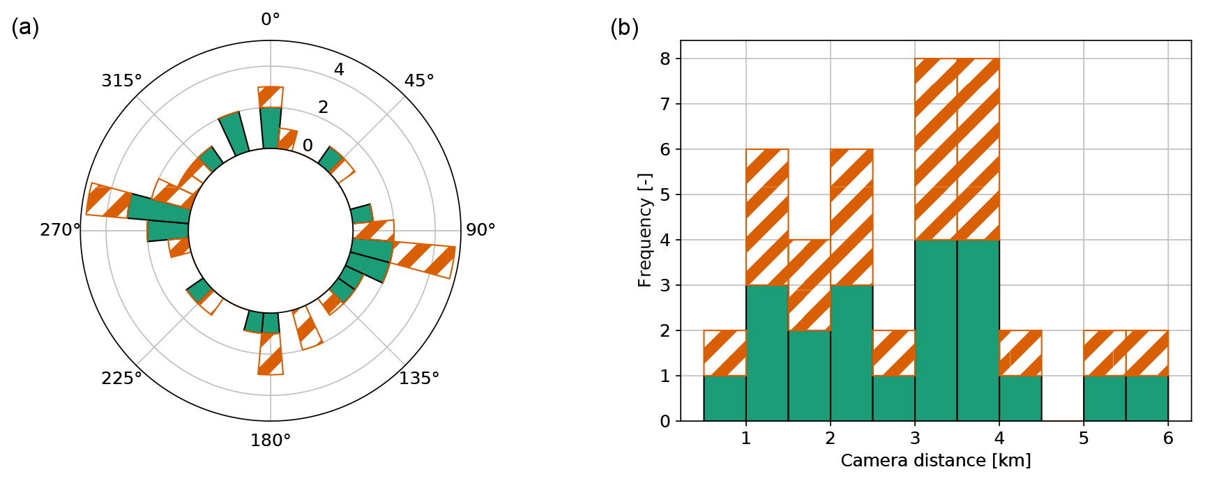
Figure 2 Frequency distribution of the bearing angles of the axes of the ASI pairs in the set of available ASI pairs (over north; a) and frequency distribution of available camera distances (b) resulting when arranging the seven ASIs in the urban area into 42 ASI pairs (from each two-ASI tuple, two different ASI pairs result by switching the main camera). The counts of ASI pairs with the switched main camera are marked with candy-striped orange.

The used Lufft CHM 15 k NIMBUS (firmware v0.747) ceilometer has been operated by the Deutsches Zentrum für Luft- und Raumfahrt (DLR) since 2018. The CBH is measured by the manufacturer's sky condition algorithm (Lufft, 2018) in the default configuration. Heese et al. (2010) specifies that, for a ceilometer of the same type, a full overlap of the laser's and the receiver's field of view is reached at a height of 1500 m. However, relying on an overlap correction, the manufacturer specifies a minimum CBH of down to 0 m. In this study, the manufacturer's default minimum CBH of 45 m is used.

The used ASIs are MOBOTIX Q25 6 MP color version surveillance cameras (Mobotix, 2017) with a fisheye lens providing a 180^∘ field of view. The ASIs are configured to use a constant exposure time of 149 µs and a constant color temperature of 5500 K. The effective image resolution is 2048 pixel × 2112 pixel. An exemplary sky image from ASI UOL is shown in Fig. 3 (left). The intrinsic calibration of the ASIs was determined according to Scaramuzza et al. (2006). The locations of the ASIs, defined by latitude, longitude and altitude, were identified in geolocated satellite images. Altitude was estimated based on the local altitude of the ground and the stations' height above the ground. The exact orientation of the ASIs' field of view was computed from the trajectory of the full Moon registered in nighttime images, as described by Nouri et al. (2019a).

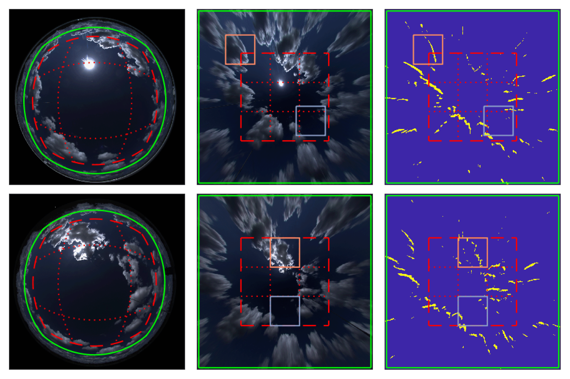
Figure 3 Sky areas evaluated in the measurement of the CBH exemplary for the ASI pair FLE-UOL, with ASI UOL in the top row and FLE in the bottom row. Shown are the maximum extent (solid green shape) and area used by the main camera in the default case (red shape, dashed line) in the distorted ASI image (left), in the undistorted orthoimage (center) and in the binary red channel difference image of two consecutive exposures (right). The binary red channel difference image (right) indicates the areas considered as being features in the cross-correlation for the comparison to the second camera with yellow shapes. A rejected match between the ASI images is marked in orange, and a valid match is marked in grayish blue.

The ASIs provide sky images at every half and full minute. The ceilometer provides readings at 0, 15, 30 and 45 s after each full minute. The clock of each measurement instrument is, at any time, synchronized via the NTP (network time protocol). Sky images, measurements of the CBH and meteorological parameters are uploaded over the cellular network to a central server, typically within 2.5 s and, in most cases, within 5 s after acquisition. A high-performance computer (HPC) is used to compute the CBH from sky images. Image processing takes up the major share of the computation time required by the presented method. These tasks are performed in parallel for each of the seven ASIs (typically allocating 4 CPUs of 3.4 GHz and 1 GB memory to each ASI), thus avoiding redundant calculations. In this way, computational cost increases mostly linearly, with the number of ASIs used instead of with the number of ASI combinations, so that execution in real time is possible. In total, including computation time, the estimation of the CBH by the ASI network can be retrieved within 10 s after image acquisition. The CBH is computed by the ASI pairs and by the ASI network during the daytime, i.e., if the Sun elevation at the time of image acquisition is greater than 0^∘.

The data set used in this study covers the period from 1 April 2019 through 27 September 2019. It is split into a period used for deriving the method (until 29 June 2019) and a period used for validations (starting from 30 June 2019). Time stamps from the validation period of 30 June 2019 to 27 September 2019 are excluded from the model development and also from the estimation of conditional probabilities.

3 Development of a CBH estimation using the ASI network

In this section, we present a procedure to estimate the CBH by an ASI network. The procedure aims to be more accurate compared to an estimation of the CBH by independent ASI pairs. First, properties of the reference CBH received from a ceilometer and properties of the CBH received from ASI pairs are discussed. Next, meteorological conditions at the site which are relevant to the performance of a CBH measurement are discussed. Based on this, we develop the estimation which borrows principles from the maximum likelihood estimation (MLE).

3.1 Properties of CBH measurements from ceilometers and from ASI pairs

As introduced in Sect. 2, a Lufft CHM 15 k NIMBUS ceilometer is used as a reference in the development and validation presented in this study. When low and optically thick clouds are present, only the lowest cloud layer is expected to be recognized reliably by the ceilometer. Therefore, in the case of overlaid cloud layers, we only evaluate readings provided for the lowest layer. This approach applies to all evaluations presented in this publication.

Regarding the accuracy of ceilometers in general, de Haij et al. (2016) and Görsdorf et al. (2016) noted that there is no generally accepted, quantifiable definition of the CBH yet. Furthermore, due to a lack of reference measurements, benchmarks may typically focus on the consistency of CBH measurements by different types of ceilometers. In a benchmark study performed by Martucci et al. (2010), the measurement of a Vaisala CL31 ceilometer CBH_CL showed a significant deviation from the reading CBH_CHM of the instrument used here. This trend was given by CBH_CL=160.315 m + 0.925×CBH_CHM. However, the measurement procedure of the instrument used here was modified by firmware updates in the meantime. Görsdorf et al. (2016) presented results from a more recent measurement campaign, CeiLinEx2015, which took place in 2015. In this experiment, the measurements of six types of ceilometers were compared. For stratus and stratocumulus clouds, as well as for fog, deviations of up to 70 m between the instruments were observed. For each of these conditions, the CHM 15 k, used here, provided the smallest measurements of the CBH in terms of mean deviation from the median of all tested instruments. More severe deviations of several kilometers between the instrument types were observed during conditions with heavy rain.

In an acceptance test, de Haij et al. (2016) measured the CBH with two CHM 15 k, a Vaisala LD40 ceilometer, a UV lidar (Leosphere ALS450) and visibility sensors mounted at various altitudes on a tower of 213 m in height. For a CBH of up to 200 m, the CHM 15 k typically measured a CBH which was 30…50 m less than the one measured by the LD40. However, the CHM 15 k was in better agreement with the estimate based on visibility sensors. Görsdorf et al. (2016) and de Haij et al. (2016) suggest that the negative mean deviation of the CHM 15 k attested to by all these studies for clouds in the range CBH<3 km is mostly caused by the manufacturers' algorithms for detecting the CBH from backscatter profiles. Where the CHM 15 k detects the rising edge of a backscatter peak that exceeds a threshold, according to the manufacturer (Lufft, 2018), other manufacturers' devices may instead recognize the peak's maximum.

For the range of the CBH in 3…12 km, an inspection of the time series depicted by de Haij et al. (2016) indicates a very good agreement of the measurements from CHM 15 k and the UV lidar used there. de Haij et al. (2016) performed a further test at a resolution of 60 s, and high clouds, detected by the UV lidar in a range of 6…7.5 km, were detected by the CHM 15 k within a tolerance of ±3 classes in the hh code (as defined by the WMO in Table 1677; World Meteorological Organization, 2019). This tolerance corresponds to a CBH range of ±1050 m centered around the discretized reference CBH. CHM 15 k attested to a probability of detection of >98 % and a false alarm rate of 0 %. Based on these studies, the accuracy of the reference instrument is expected to be adequate for the range of CBH<3 km. Also, for the range of CBH≥3 km, a rather good performance of the instrument is indicated. The experimental results of this study will, in particular, be compared to prior studies which used a ceilometer of the same type. This is expected to avoid possible inconsistencies related to the used reference.

From all ASIs available in the urban area, we form independent ASI pairs that measure the CBH by a stereoscopic triangulation, which was introduced by Kuhn et al. (2018b) and further refined by Nouri et al. (2019a). The algorithm used here to estimate the CBH by the individual ASI pairs has been described and validated in the latter publication. Nouri et al. (2019a) evaluated an ASI pair with a camera distance of 495 m. For four ranges of the reference CBH, defined by the bin edges $\mathrm{0},\mathrm{3},\mathrm{6},\mathrm{9},$ and 12 km, root mean squared deviations (RMSDs) of $\mathrm{0.6},\mathrm{1.4},\mathrm{3.2},$ and 3.1 km were found for 10 min averaged CBH. The study did not provide information on bias. Furthermore, in that validation, higher clouds were more frequent, and no observations at a reference CBH of less than 1 km occurred. The studies of Kuhn et al. (2018b) and Nouri et al. (2019a) were performed in Almería, Spain. Both studies validated the ASI-based measurement of the CBH using a Lufft CHM 15 k ceilometer as a reference. At this point, we recapitulate aspects of the procedure which are important for the remaining publication. For a more detailed description, we refer to Nouri et al. (2019a).

Images from both ASIs (e.g., UOL and FLE; see the left-hand side of Fig. 3) are first projected into horizontal planes yielding orthogonal images (Fig. 3; center) by a well-established method described, e.g., by Luhmann (2000). Then, the difference in the red channel, compared to the image recorded 30 s before, is calculated for the image of each ASI. Areas in the difference images of the two cameras, where the red channel changes most significantly (98 percentile) within the 30 s between consecutive images, are used as features (illustrated in Fig. 3; right) to be matched by block-wise correlation. With the known camera distance, a shift received in the cross-correlation is translated into a height of the feature above the ground.

In practice, the triangulation relies on cloud edges which are visible from both perspectives and provide sufficient contrast. Therefore, the method responds stronger to optically dense clouds, especially in the proximity of the Sun, as found by Kuhn et al. (2018b). Moreover, we do not measure the CBH exactly but rather the height of these distinct cloud edges. We expect to introduce a small bias when using this cloud height as the CBH. Nouri et al. (2019a) analyzed sources of deviations when estimating the CBH by an ASI pair. In accordance with that study, we expect this bias to be acceptable when compared to other uncertainties and to be of the order of 100 m.

In accordance with the system used by Nouri et al. (2019a), we use a cascading procedure to estimate the CBH robustly and also in conditions with low sky coverage. First, the main ASI's orthogonal image is restricted to a square-shaped area (Fig. 3; red shape, dashed line) defined by a maximum zenith angle of 67^∘, measured in the center of each side of the square. In a cross-correlation, each of the nine squares confined by dotted or dashed lines (also known as windows; Fig. 3; bottom right) from the orthoimage of the main ASI is matched with an area with an identical shape from the orthoimage of the second ASI (Fig. 3; top right). With the known camera distance, the shift is converted into a measurement of the CBH.

If the estimation of the CBH failed for one of the windows, valid readings from neighboring ones are averaged, ignoring any window for which the estimation failed. In cases with no valid measurement in any of the windows, the orthogonal images of both ASIs are evaluated up to a maximum zenith angle of 77.8^∘ (measured at the center of each image side; green shapes in Fig. 3). These orthoimages from both cameras are matched in the cross-correlation, and the ASI pair returns a uniform CBH. This second step can yield a valid measurement of the CBH in cases when only few clouds are present to be matched. This step mainly intends to increase the robustness of the CBH measurement. This step is not expected to increase the ability of an ASI pair to detect very low clouds in relation to the camera distance, as the window size used in this step is very large.

As a modification of the method by Nouri et al. (2019a), we only use the CBH provided for the central point of the orthoimage of the main ASI corresponding to a zenith angle of 0^∘. This procedure is followed for both the ASI pairs and for the ASI network using these ASI pairs. We expect that an ASI-based measurement of the CBH is most accurate for this central point. This point receives the CBH primarily from matches involving the central window of the main ASI's orthoimage, which is less affected by image distortion. The central window of the main ASI's orthoimage covers zenith angles up to 38.1^∘, which are measured at the center of each window side. Thus, a CBH measurement for a square-shaped area around the main ASI's location is yielded. For example, the area's side lengths measure 1.6, 4.7, 7.8 and 15.7 km for a respective CBH of 1, 3, 5 and 10 km. When only based on geometry and the evaluated image areas, this central window could provide readings down to a minimum CBH of 0.25×d, where d is the camera distance. However, under such extreme conditions, the matching procedure may fail very frequently. The central peripheral windows, shown in Fig. 3, approximately cover the zenith angles 38.1…67^∘. The matched area from the auxiliary ASI's orthogonal image has an identical shape and can cover a zenith angle up to 77.8^∘. Based on this, we estimate the minimum CBH, which an ASI pair can measure, to be 0.18×d. However, in our experience, a large fraction of clouds observed at zenith angles larger than 67^∘ are not matched successfully between the ASIs and are typically rejected. In the case that the matching procedure could only be successful if the second ASI's window also included zenith angles not larger than 67^∘, then the CBH could be measured down to 0.32×d, using the peripheral windows, and 0.64×d, using the central window.

This central point of the orthoimage, used here, was also the focus of the validation presented by Nouri et al. (2019a), as the ceilometer was placed at one ASI's location, and the observed CBH values were not smaller than 1 km. Overall, we expect that, by applying cross-correlation to binary difference images, our measurement approximates the median CBH of the cloud layer that is locally most dominant in features driven by area and optical thickness.

A previous study by Kuhn et al. (2019) showed that the camera distance and the CBH itself significantly influence the accuracy received in the measurement of the CBH by an ASI pair with the present approach. Based on this, we use camera distance and the CBH to characterize ASI pairs.

3.2 Meteorological conditions at the site

To understand the performance of the CBH measurement based on ASI pairs, we briefly analyze the on-site meteorological conditions based on ceilometer and ASI data. Using ASI UOL, we study the dominant directions of cloud motion at the site. Nouri et al. (2019a) found a RMSD of 17^∘ for the estimation of the direction of cloud motion based on an ASI pair. Based on this, we consider the estimation of cloud motion directions from ASI UOL as being sufficiently accurate for this statistical evaluation. Figure 4 (left) shows the distribution of cloud motion directions estimated with the ASI in the sense of a wind rose representing the directions from which clouds approach the urban area. Seen are two main lobes at azimuthal angles of 240^∘ N (west to southwest) and 290^∘ N (west to northwest), while other directions of cloud motion are observed rather seldom.

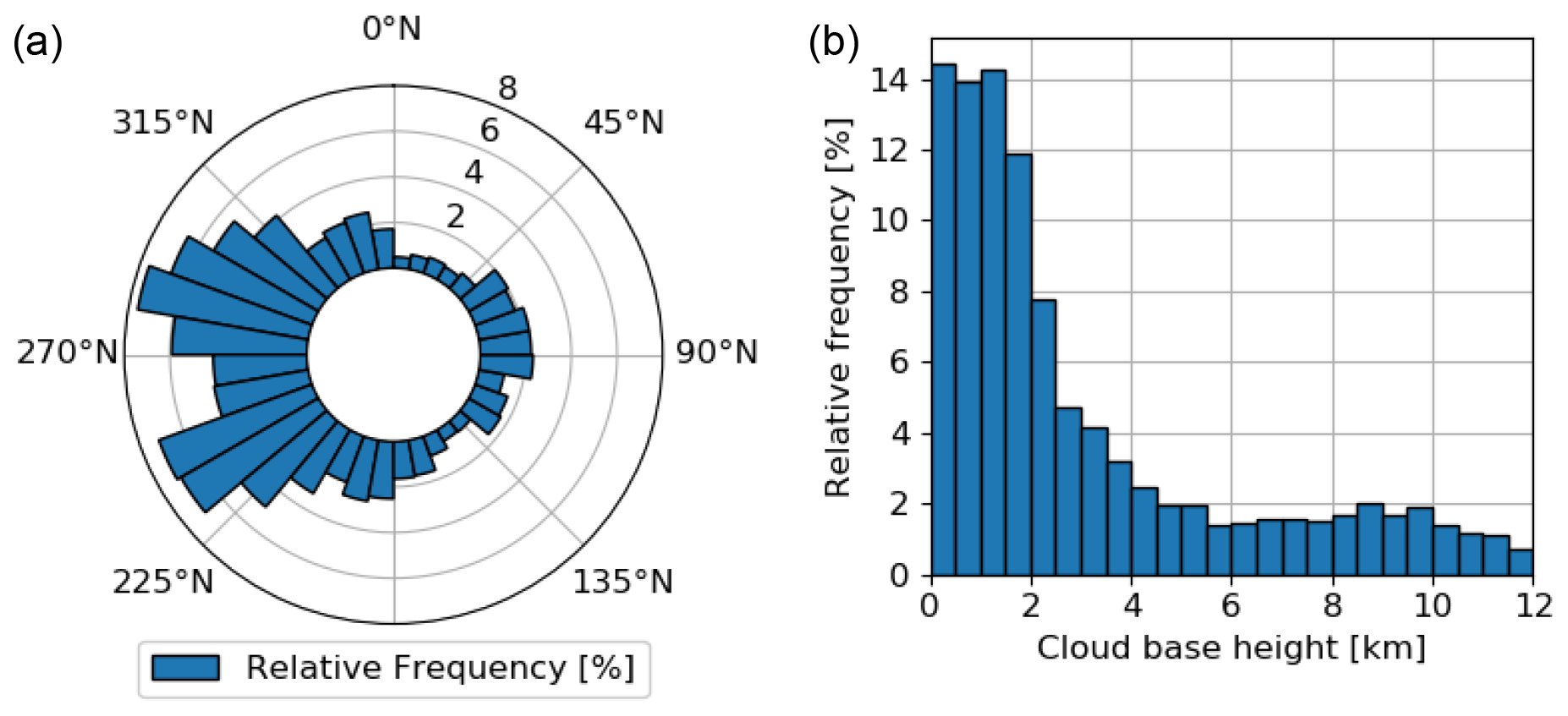
Figure 4 Wind rose of cloud motion directions derived from ASI UOL, indicating a dominance of clouds coming from western directions (a), and the distribution of the cloud base height (CBH) in the analyzed period (b).

The distribution of the CBH at the site of Oldenburg for the full measuring period is given in Fig. 4 (right). As in general in this study, the analysis is based only on the lowest cloud layer detected by the ceilometer. The majority of all ceilometer readings (54 %) indicates a CBH smaller than 2 km. Similarly, within the interval $\mathrm{CBH}\in ]\mathrm{0},\mathrm{2}[$ km, all values are observed with a similar frequency. This includes the lowest bin of $\mathrm{CBH}\in ]\mathrm{0},\mathrm{0.5}[$ km, which indicates conditions with fog or low stratus clouds. For the majority of situations, it is of special interest to receive accurate measurements in the low range of the CBH. Moreover, 28 % and 18 % of readings are found, respectively, in the intermediate range of $\mathrm{CBH}\in [\mathrm{2},\mathrm{6}[$ km and in the range of large $\mathrm{CBH}\in [\mathrm{6},\mathrm{12}[$ km. Within the range of high clouds, a roll-off of the frequency is seen for CBH>10 km. A reliable estimation of the CBH should, therefore, provide accurate readings for the range of $\mathrm{CBH}\in ]\mathrm{0},\mathrm{12}[$ km.

A visual analysis and a k-means classification for the site of Oldenburg (not shown) suggested that local conditions predominantly feature distinct cloud layers with temporally low vertical variability. The major cause of the variable CBH is found in the transitions between cloud layers. It is concluded that, for sites with similar meteorological conditions, it is most important to measure the CBH of the cloud layer which is the most dominant at the evaluated time as accurately as possible. Kottek et al. (2006) characterize the climate in Oldenburg as warm temperate, fully humid with warm summers (Cfb). In this publication, a summer half-year period (April–September) is studied. The climate is strongly influenced by the North Sea which is located at a distance of roughly 70 km. Eye2Sky, and especially Oldenburg, are situated in a plane with a maximum elevation above sea level of less than 160 m, including vegetation and human infrastructure, which we calculated from the TanDEM-X elevation model (Wessel et al., 2018). The flat topography is expected to support a temporally and spatially low variability in the CBH within cloud layers. For other sites, a focus on measuring the CBH for every cloud object is of higher priority. For example, Tabernas, Spain, the site studied by Nouri et al. (2019a), features a cold arid (steppe) climate (BSk according to Kottek et al., 2006) and is surrounded by mountains with elevations up to 2168 m above sea level within a radius of 25 km. As shown by (Nouri et al., 2019c), the CBH at the site is distributed almost uniformly in the range 0…11 km. These characteristics are expected to cause greater temporal and spatial variability in the CBH. To conclude, a procedure, which estimates the CBH of the cloud layer most dominant in the urban area of Oldenburg accurately, is considered beneficial for assessing and modeling clouds in the same area (depicted in Fig. 1; right). Still, if clouds over the whole region covered by Eye2Sky (depicted in Fig. 1; left) are assessed, this method alone may not be sufficient. In the future, local cloud conditions may be classified by image processing techniques (e.g., Fabel et al., 2021), and the CBH may be assigned to local clouds from clouds of the same type, which were recently observed in the urban area.

3.3 Estimating the CBH in the ASI network

In this section, we present our method for combining the measurements of the CBH from a large number of ASI pairs organized as a network. Prior works estimated the CBH from a small number of two or, in some cases, four ASIs (Nouri et al., 2019a). However, with a large number of ASI pairs, we consider a statistical method promising, as it analyzes the CBH samples received and, based on the known characteristics of each ASI pair, determines the CBH which is most likely to be present. The characteristics of each ASI pair are, in the following, described by conditional probability distributions, which will be discussed in Sect. 3.4. These distributions provide the probability of receiving a certain CBH reading from an ASI pair, given that actually a specific reference CBH is present. Our estimation procedure then uses principles from a maximum likelihood estimation (MLE) and modifies them for the specific case. To the best of our knowledge, the usage of a statistical method and, in particular, one relying on conditional probability distributions is novel to the task of estimating the CBH from the observations of a multitude of ASIs.

To give an overview, Fig. 5 shows the inference process used to estimate the CBH by the network based on the 42 CBH readings provided by the individual ASI pairs. For each range i of camera distance, in Sect. 3.4, conditional probability distributions will be estimated. These conditional probabilities are translated into the likelihood that, actually, certain values of the (reference) CBH are present (step 1) based on the readings of the CBH received from ASI pairs in this range i of camera distance. After calculating the cumulative likelihood for each range of camera distance (step 2), these are combined, yielding the overall cumulative and complementary cumulative likelihood from all ASI pairs (step 3). Finally, the value of the CBH which is most likely to be present at the site and at the evaluated time, given the readings from all involved ASI pairs, is estimated (step 4). These steps are presented in more detail in the following.

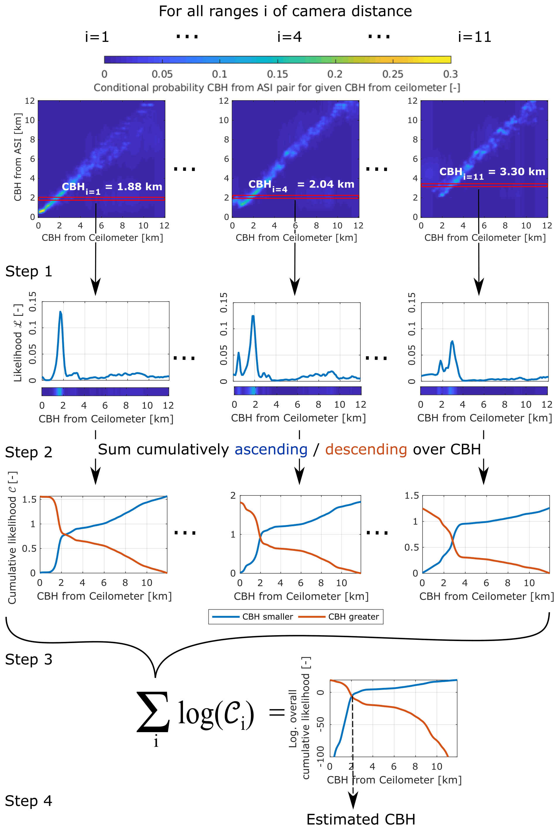
Figure 5 A flow diagram of the inference procedure. In step 1, for each range i of camera distance, CBH_i is computed as the mean CBH from the respective ASI pairs. True CBH (at the ceilometer; unknown in the inference) is set to a value in {0… 0.1,0.1… 0.2,… ,11.9… 12} km (red boxes), one by one. Given the respective true CBH, the conditional probability of receiving CBH_i is computed. Step 1 yields a likelihood function for each range of camera distance. In step 2, the cumulative and complementary cumulative likelihood are calculated for each range of camera distance. In step 3, these functions are turned into a logarithm and then summed over all ranges i of camera distance, yielding the overall cumulative and complementary cumulative likelihood. In step 4, the intersection of both functions gives the estimation of the likeliest CBH.

In step 1, for each ASI pair, the median value of all valid CBH readings of the previous 10 min is calculated. If an ASI pair does not provide any valid CBH within this period, it is excluded from the prediction for the instance in time evaluated. The ranges of camera distance, 1…2.5 and 3…4 km, are represented by a larger number of ASI pairs than the remaining distances. Thus, the readings of the ASI pairs in these ranges of camera distance may prevail in the estimation of the CBH. As the variety of camera distances is considered to benefit the procedure, we intend to represent all camera distances as uniformly as possible. Thus, we define ranges of camera distance using the range limits of $\mathit{\{}\mathrm{0.5},\mathrm{1},\mathrm{1.5},\mathrm{\dots },\mathrm{6}\mathit{\}}$ km. The CBH readings of all ASI pairs with camera distance in range i are averaged to yield CBH_i. Consecutively, the conditional probability P(CBH_i | h_true) is evaluated so that the found CBH_i would be received for a given true CBH h_true (box marked red prior to step 1 in Fig. 5). Note that P(CBH_i | h_true) will be modeled in Sect. 3.4 using h_Ref measured by a ceilometer which provides h_Ref≈h_true. Thus, the likelihood ℒ_i(h_true) is obtained as follows (Fig. 5; output of step 1):

$$\begin{array}{}\text{(1)}& {\mathcal{L}}_i\left(h_{\mathrm{true}}\right)=P\left({\mathrm{CBH}}_i\right|h_{\mathrm{true}}).\end{array}$$

In step 2, we define the cumulative likelihood ${\mathcal{C}}_i\left({\widehat{h}}_{\mathrm{true}}\right)$ as the likelihood of receiving the present reading CBH_i given that h_true is smaller than or equal to an estimation of the true CBH ${\widehat{h}}_{\mathrm{true}}$. Accordingly, in the implementation, the likelihood is summed cumulatively over all bins of the reference CBH h_true as follows (Fig. 5; step 2):

$$\begin{array}{}\text{(2)}& {\mathcal{C}}_i\left({\widehat{h}}_{\mathrm{true}}\right)=\sum _{h_{\mathrm{true}}\le {\widehat{h}}_{\mathrm{true}}}{\mathcal{L}}_i\left(h_{\mathrm{true}}\right).\end{array}$$

Likewise, a complementary cumulative likelihood is defined as the likelihood of receiving the present reading CBH_i, given that h_true is greater than an estimation of the true CBH ${\widehat{h}}_{\mathrm{true}}$, as follows:

$$\begin{array}{}\text{(3)}& {\stackrel{\mathrm{‾}}{\mathcal{C}}}_i\left({\widehat{h}}_{\mathrm{true}}\right)=\sum _{h_{\mathrm{true}}>{\widehat{h}}_{\mathrm{true}}}{\mathcal{L}}_i\left(h_{\mathrm{true}}\right).\end{array}$$

In particular, the use of these cumulative functions and the estimation of likelihood functions from measurement data distinguish the present approach from a regular MLE. This modification is used as, in MLE, typically smooth analytical functions are assumed as likelihood function. In contrast, likelihood functions here will be estimated based on empirical conditional probabilities. These approximated likelihood functions, derived from a data set of finite size, may therefore be less smooth and may not be completely representative. When using cumulative distributions, it is expected that the method still works robustly if the conditional probabilities are not estimated accurately for each grid cell of the discrete distribution if at least the cumulative value over a range of CBHs is appropriate. In spite of the modification, the presented approach may adopt beneficial properties of MLE. The use of appropriate conditional probabilities (determined in Sect. 3.4) reduces the systematic deviations of the estimated CBH compared to the measurement of a single ASI pair. Moreover, applied conditional probabilities are, in general, not specific to the studied site and its meteorological conditions, which allows us to apply the method at other sites. Both functions ${\mathcal{C}}_i\left({\widehat{h}}_{\mathrm{true}}\right)$ and ${\stackrel{\mathrm{‾}}{\mathcal{C}}}_i\left({\widehat{h}}_{\mathrm{true}}\right)$ are shown for three exemplary intervals of camera distance in Fig. 5 as an output of step 2.

In step 3, we aim to determine the likelihood of receiving the combination of readings CBH_i from all the intervals i of camera distance, given that $h_{\mathrm{true}}\le {\widehat{h}}_{\mathrm{true}}$. This can be expressed as a product of ${\mathcal{C}}_i\left({\widehat{h}}_{\mathrm{true}}\right)$ from all intervals i. As this product would often become zero in our numerical treatment, we instead calculate its natural logarithm, which we refer to as overall logarithmic cumulative likelihood of $\log {\mathcal{C}}_n\left({\widehat{h}}_{\mathrm{true}}\right)$. This operation also allows us to replace the product by a sum, as follows (Fig. 5; step 3):

$$\begin{array}{}\text{(4)}& \log {\mathcal{C}}_n\left({\widehat{h}}_{\mathrm{true}}\right)=\sum _i\log {\mathcal{C}}_i\left({\widehat{h}}_{\mathrm{true}}\right).\end{array}$$

Analogously, an overall complementary logarithmic cumulative likelihood is computed, given all the readings CBH_i per interval i of camera distance, as follows:

$$\begin{array}{}\text{(5)}& \log {\stackrel{\mathrm{‾}}{\mathcal{C}}}_n\left({\widehat{h}}_{\mathrm{true}}\right)=\sum _i\log {\stackrel{\mathrm{‾}}{\mathcal{C}}}_i\left({\widehat{h}}_{\mathrm{true}}\right).\end{array}$$

Both functions are visualized exemplarily as outputs of step 3 in Fig. 5.

In step 4, $\log {\mathcal{C}}_n\left({\widehat{h}}_{\mathrm{true}}\right)$ and $\log {\stackrel{\mathrm{‾}}{\mathcal{C}}}_n\left({\widehat{h}}_{\mathrm{true}}\right)$ are only known at discrete points, and a linear interpolation yields continuous representations of these functions. Then, finally, we aim to select the true CBH h_likeliest, which makes it the likeliest to receive the given combination of CBH_i. In our formulation of the problem, this means that we intend to find a ${\widehat{h}}_{\mathrm{likeliest}}$ which simultaneously maximizes $\log {\mathcal{C}}_n\left({\widehat{h}}_{\mathrm{true}}\right)$ and $\log {\stackrel{\mathrm{‾}}{\mathcal{C}}}_n\left({\widehat{h}}_{\mathrm{true}}\right)$. Consequently, we accept h_likeliest, for which $\log {\mathcal{C}}_n\left({\widehat{h}}_{\mathrm{true}}\right)$ and $\log {\stackrel{\mathrm{‾}}{\mathcal{C}}}_n\left({\widehat{h}}_{\mathrm{true}}\right)$ are equal, as follows (Fig. 5; step 4):

$$\begin{array}{}\text{(6)}& h_{\mathrm{likeliest}}=\underset{{\widehat{h}}_{\mathrm{true}}}{\text{argmin}}\left|\log {\stackrel{\mathrm{‾}}{\mathcal{C}}}_n\left({\widehat{h}}_{\mathrm{true}}\right)-\log {\mathcal{C}}_n\left({\widehat{h}}_{\mathrm{true}}\right)\right|.\end{array}$$

Besides this estimation of the CBH, a version of this procedure will be discussed that includes further refinements (referred to in the following as the refined estimation). As a first observation from the generation of conditional probabilities, ASI pairs with a camera distance greater than 4.5 km cause large deviations for CBH<4 km and exhibit only a moderate advantage at a greater CBH. These ASI pairs are excluded from the refined estimation of h_likeliest. On the other hand, ASI pairs with a small camera distance are already accurate if only small CBHs occur, as we will discuss in Sect. 4. We inspected the conditional probabilities of the ASI pairs (exemplarily viewed as input to step 1 in Fig. 5) and identified the ASI pairs which are most appropriate for an interval of the CBH. Based on this, the refined estimation is received from the arithmetic average of the CBH measured by ASI pairs with corresponding small camera distance, if the first iteration of h_likeliest yielded a sufficiently small CBH. In summary, the refinement procedure for receiving the final estimation of the CBH h_refined reads as follows:

$$\begin{array}{}\text{(7)}& {\displaystyle }{h}_{\mathrm{refined}}\left\{\begin{array}{ll}{h}_{\mathrm{likeliest}},& h_{\mathrm{likeliest}}\in ]\mathrm{3},\mathrm{12}]\mathrm{km}\\ min(\mathrm{3}\mathrm{km},\text{mean}(h_{i\in \mathit{\left\{}i\right|d_i<\mathrm{1.6}\mathrm{km}\mathit{\}}}\left)\right),& h_{\mathrm{likeliest}}\le \mathrm{3}\mathrm{km}\wedge \text{mean}\left(h_{i\in \mathit{\left\{}i\right|d_i<\mathrm{1.6}\mathrm{km}\mathit{\}}}\right)>\mathrm{1.5}\mathrm{km}\\ min(\mathrm{1.5}\mathrm{km},\text{mean}(h_{i\in \mathit{\left\{}i\right|d_i<\mathrm{1.2}\mathrm{km}\mathit{\}}}\left)\right),& h_{\mathrm{likeliest}}\le \mathrm{3}\mathrm{km}\wedge \text{mean}\left(h_{i\in \mathit{\left\{}i\right|d_i<\mathrm{1.6}\mathrm{km}\mathit{\}}}\right)\le \mathrm{1.5}\mathrm{km}.\end{array}\right.\end{array}$$

3.4 Estimation of conditional probabilities of the CBH

The procedure to combine the CBH measurements from independent ASI pairs, which are organized as a network, requires knowledge of the (conditional) probability of receiving a certain reading of the CBH from an ASI pair given that the true CBH takes on some specific value. The required distribution aims to answer the following question: if the true CBH ranges between 1.8…1.9 km, how large will the probability be that an ASI pair with camera distance 2.2 km delivers a certain CBH, e.g., within 0…0.1 km, 1.8…1.9 km or 11.9…12 km? In the following, these conditional probabilities are estimated not only for the range of the true CBH between 1.8 and 1.9 km but for each range, i.e., $\mathit{\{}\mathrm{0}\mathrm{\dots }\mathrm{0.1},\mathrm{0.1}\mathrm{\dots }\mathrm{0.2},\mathrm{0.2}\mathrm{\dots }\mathrm{0.3},\mathrm{\dots },\mathrm{11.9}\mathrm{\dots }\mathrm{12}\mathit{\}}$ km, of the true CBH. Conditional probability distributions of this kind are not available so far for ASI pairs. Therefore, we aim to approximate them from the measurement data of a modeling period. Estimations of the CBH from the available ASI pairs and measurements from the ceilometer during the period 1 April 2019 to 29 June 2019 are used. The CBH measured by the ceilometer serves as the reference CBH. It is not considered to be essential that the training period is representative of the period to which the method is applied. However, we expect that the method works best if the included ASI pairs exhibit a similar distribution of measurement deviations given the same reference CBH in both periods. For solar applications and the latitude of this study, we consider the used data set and its split reasonable. The summer and shoulder months provide the main share of the annual solar yield at the site and are therefore the focus of the nowcasting system under development. In that sense, the training data set is considered to be, for the most part, representative of conditions relevant to solar applications at similar latitudes.

The seven ASIs available in the urban area are arranged into 42 ASI pairs. Each tuple of two ASIs that is selected from the set of seven ASIs yields two independent ASI pairs by swapping the ASI used as a main camera (see Sect. 3.1).

The procedure is developed based on periods in which valid measurements from ceilometer and the respective ASI pair are available and in which the variability in the CBH is moderate. For each time stamp, a window of 30 min centered at this time stamp is defined. A time stamp is only included if the standard deviation of the reference CBH within the window is less than 30 % of the mean value of the reference CBH within the same window. As discussed before, the ASI pairs and ceilometer measure the CBH as a spatial median and point-wise, respectively. Therefore, this filter intends to assure that the ceilometer and ASI pair measure the CBH of the same layer. The CBH from the respective ASI pair and from the ceilometer are processed by a moving median filter with a window of 10 min. The joint frequency distribution of the CBH measured by ceilometer h_Ref and the respective ASI pair h_ASI is computed from these simultaneously acquired time series. In other words, the domain of reasonable values, $[\mathrm{0},\mathrm{12}\mathrm{km}[\times [\mathrm{0},\mathrm{12}\mathrm{km}[$, which the pair (h_Ref,h_ASI) can take on, is discretized into a mesh of square grid cells with side lengths Δh. Then the frequency is calculated with which (h_Ref,h_ASI) is observed in each of the discrete grid cells. A bin size Δh=100 m is chosen in a trade-off between sources of error. Finer bins will allow one to represent the distributions at higher resolution and will, thus, allow for higher resolved measurements of the CBH in the network. However, the size of the used data set is limited, which makes it difficult to model these distributions at the highest resolution. The bin size chosen here is expected to limit the achievable uncertainty of the measurement to a minimum level of 100 m.

Joint frequency distributions were inspected and found to be well reproduced among the studied independent ASI pairs as long as the corresponding camera distances are similar. This meets the expectation from the literature discussed in Sect. 3.1. Moreover, we conclude that the distributions modeled here will be transferable to other setups that use camera distances in the studied range. Local climate is expected to influence the transferability to a minor extent.

The limited size and representativeness of the data set used in the model development are expected to cause random features in the joint frequency distributions which are not useful for the estimation procedure when it is applied to other setups, sites and times (such as those represented by the validation data set). To suppress such random features of received joint frequency distributions, we introduce a filtering procedure with two consecutive steps described here and in more detail in Appendix A. The parameter values set in the filtering procedure are approximate to this point and are based on a visual comparison of unfiltered and filtered distributions. The comparison evaluated the degree to which noise, but also reasonable features, was suppressed. The parameters values may be optimized in a future study.

First, a weighted mean filter is applied between the original joint frequency distributions received for ASI pairs with similar camera distance. As discussed above, ASI pairs with a similar camera distance are expected to perform similarly in the measurement of the CBH and should, consequently, also exhibit similar joint frequency distributions in the CBH. Thus, the filter aims to suppress differences between the joint frequency distributions of ASI pairs which may result from disturbances in the estimation rather than from a difference in the systems' characteristics.

To each filtered distribution resulting from the prior step, a composite of three Gaussian filters is applied. We first decompose each distribution by conditional filters into three separate modes which correspond to parts of the joint frequency distributions that are estimated with descending precision. Thereafter, we apply a Gaussian filter to each mode. The standard deviation of the Gaussian filter applied to each mode corresponds qualitatively to the uncertainty with which the prior joint frequency distribution is estimated within grid cells of that mode. Consecutively, the three filtered modes are summed to receive the smoothed joint frequency distribution.

The first mode is constituted by grid cells for which the ASI-pair-based measurement of the CBH deviates by more than 1.5 km from the ceilometer reading. The large deviations represented by this mode occur less frequently, which is why the joint frequency distribution will be estimated less precisely for the respective grid cells. On the other hand, apart from such scattering effects, the joint frequency distributions are found to be comparably smooth in the grid cells of this mode. A Gaussian filter with a large standard deviation of 1 km is applied to this mode, which is considered to be apt for preserving the expected distribution while suppressing random features.

The second mode is constituted by grid cells for which the ASI-pair-based measurement of the CBH deviates by less than 1.5 km from the ceilometer reading and which feature a joint frequency below the average of all grid cells. These grid cells typically exhibit a larger joint frequency, i.e., more observations, than grid cells in the first mode. Still the comparably small number of observations in these grid cells is expected to cause an increased uncertainty in the estimated joint frequencies. Consequently, in a trade-off between suppressing random scattering and preserving meaningful variations, a Gaussian filter with a standard deviation of 0.5 km is applied.

The third mode makes up the complement of the first and second mode. It contains grid cells that are observed with an, at least, average joint frequency and which are not classified as outliers. Joint frequencies in these grid cells are considered to be estimated with a comparably high accuracy. To avoid a loss of precision and, ultimately, a loss of accuracy in the estimation of the CBH, a Gaussian filter with a standard deviation of 0.1 km is used. Hence, only neighboring grid cells have a significant influence on this filter.

In many joint frequency distributions, there are grid cells with a joint frequency close to zero. Especially for these grid cells, a greater data set would be required to receive more representative values. For all grid cells, joint frequency is increased to a minimum value of 0.5 to avoid underestimations of joint frequency. This value corresponds to half of the joint frequency associated with a single actual observation in a grid cell. For the estimation procedure of the CBH, such a minimum value leads to slightly reduced precision for most readings but increased robustness in the case that these grid cells (h_Ref,h_ASI) are indeed observed in the measurement. Finally, from each joint frequency distribution, the conditional probability P(h_ASI | h_Ref) of receiving a certain CBH reading from an ASI pair, given that the ceilometer measures some certain CBH, is derived (see Appendix A for a more detailed description).

The inference procedure, which was introduced in Sect. 3.3, represents each range i of camera distance bounded by the limits of $\mathit{\{}\mathrm{0.5},\mathrm{1},\mathrm{1.5},\mathrm{\dots },\mathrm{6}\mathit{\}}$ km by a single distribution of conditional probability. For each range of camera distance, the distribution of conditional probability, which corresponds to the camera distance closest to the center of this range, is selected (example provided in Appendix A). Figure 5 (above step 1) shows the exemplary conditional probabilities for three ASI pairs with camera distances of 0.8, 2.2 and 5.7 km representing the ranges of camera distance i=1, 4 and 11, respectively. Bias and precision, with which the ASI pairs of distinct camera distances measure the CBH, given a certain reference CBH, are visible in these conditional probabilities. Such characteristics will be evaluated in more detail in the following, based on a separate validation data set.

4 Validation of the CBH measurement by the ASI network and comparison to the CBH measurements by the ASI pairs

In this section, the accuracy of the CBH measurement by the ASI network and by 42 independent ASI pairs set up with a wide variety of camera distances and alignments is compared. This section is based on a validation data set including the days from 30 June 2019 to 27 September 2019. This data set was excluded from the model development described in Sect. 3. The analyzed quantity is the 10 min median CBH.

First, characteristics of the CBH measurements from the ASI network and from individual ASI pairs are compared to the CBH measurement of the reference ceilometer based on insightful days. Then, the measurements of the CBH by the ASI network and ASI pairs are compared to the one of the ceilometer by means of scatter density plots. Subsequently, the accuracy of an ASI pair and of the ASI network is analyzed for the application of the nowcasting of solar irradiance. Finally, deviation metrics of the CBH received from the network and from all individual ASI pairs per interval of the CBH are discussed.

4.1 Comparison of the CBH measurements for an exemplary day

We first analyze the properties of the different procedures to measure the CBH based on exemplary situations. Figure 6 visualizes time series of the CBH for a variable day (2 September 2019) measured by ceilometer, by all available ASI pairs and by the ASI network. The time series of two exemplary ASI pairs DON-MAR and CLO-FLE, with respective camera distances 0.8 and 4.2 km, are plotted. The range of the CBH readings covered by all available ASI pairs is shaded in gray in the figure.

Figure 6 Time series of cloud base height for an exemplary day (2 September 2019) measured by 42 ASI pairs (gray filled), by two exemplary ASI pairs, DON-MAR and CLO-FLE, with respective camera distances 0.8 and 4.2 km, by the ASI network with refinements and by a ceilometer in the urban area of Oldenburg.

In the morning (06:00 UTC; hereafter, all times are given in universal coordinated time), both ceilometer and the ASI network recognize adequately a high cloud layer. The ASI pairs with valid measurements deliver similar estimations of the CBH. Around 07:00, the ceilometer still recognizes the high layer, whereas many ASI pairs and the ASI network recognize the approaching cumulus clouds. These already cover a significant fraction of the sky in the urban area (compare Fig. 7; left). The CBH estimation approach tends to react stronger to clouds in this area of the sky in which contrasts are typically pronounced. Around 10:20, a multilayer situation is present. In all parts of the sky dome, cumulus clouds are visible but a large fraction of the cloud cover is made up by the cirrus layer. Around this time, the measurements of the ceilometer and ASI network coincide well. All ASI pairs recognize a rather low cloud layer, while there are periods in which the ceilometer recognizes the cirrus layer. All of the ASI-based CBH estimations react stronger to the low layer and miss the high layer clouds. These two situations express well why the ASI-based estimations of the CBH are less accurate for higher clouds and tend to be negatively biased. On the other hand, for low clouds, a high accuracy of the combined CBH estimation is demonstrated. Meanwhile, it is visible that, for low clouds, many ASI pairs, such as the ASI pair CLO-FLE, tend to overestimate the CBH. In these conditions, the ASI network manages to follow appropriate estimations well.

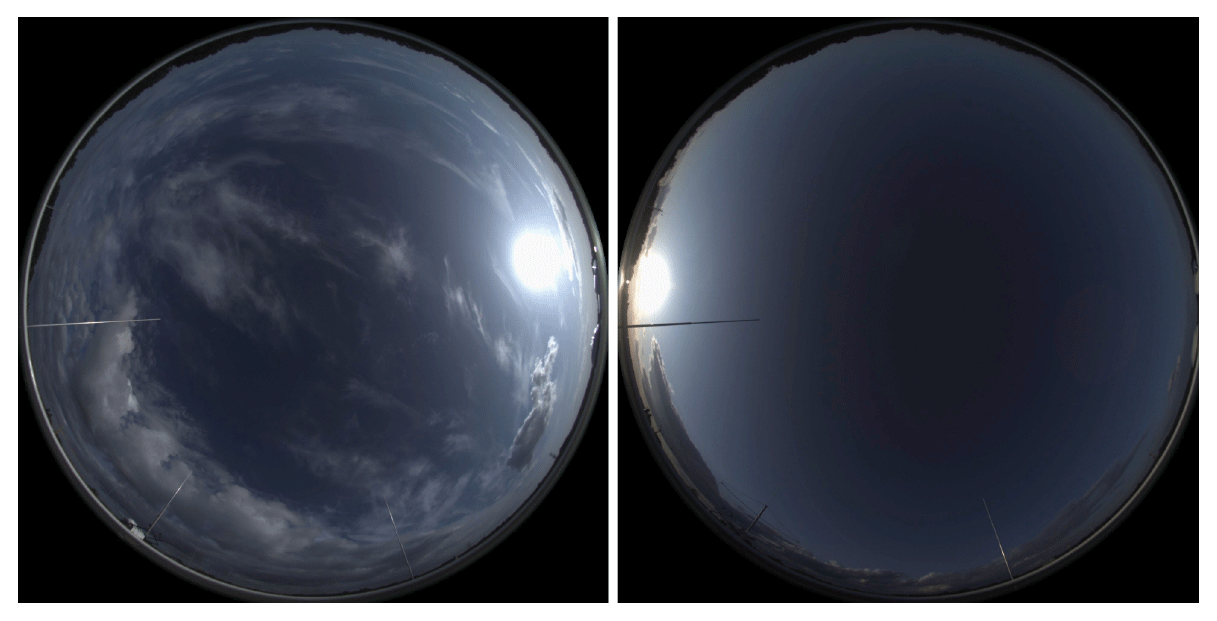
Figure 7 Sky images taken by ASI UOL, representing a multi-cloud-layer situation on 2 September 2019 07:20 (left) and an almost-clear-sky situation on 2 September 2019 17:00 (right), respectively.

Around 17:00, a nearly clear sky is visible (compare Fig. 7; right). Consequently, the ceilometer does not provide any valid CBH. The ASI pairs provide a CBH that scatters over a wide range, while the ASI network provides an intermediate CBH. A similar reading of the CBH is also recognized by a fraction of the ASI pairs. From around 17:05, the ASI network detects a CBH of 3 km. With 3.1 km, the following CBH measurements of the ceilometer at around 17:25 confirm the suggested CBH of the approaching cloud layer (see Fig. B1 for a detailed view of the CBH measurements during this almost clear sky period). This situation reflects the expected behavior of the ASI network under mostly clear conditions. However, for a completely clear sky, the ASI network partly produces invalid readings (NaN), and it partly detects a large CBH of around 10 km. In this case, a consecutive image processing step detects the absence of clouds. This step is not part of the present study.

The time series of the CBH from DON-MAR and CLO-FLE demonstrate the properties of ASI pairs with, respectively, small and large camera distances. DON-MAR is typically close to the reference CBH if it actually takes on a value below 4 km (e.g., 2 September 2019; 09:00–13:00), while this ASI pair tends to take on large deviations and a negative bias for the larger CBH (e.g., 2 September 2019; 06:00–09:00). The ASI pair of CLO-FLE typically misses the CBH of low clouds and provides a significantly overestimated CBH (e.g., 2 September 2019; 09:00–13:00). For high clouds, however, the CBH measured by CLO-FLE often coincides well with the reference. To give further insight, in Appendix B2, time series of the CBH from the different sources are compared for another exemplary day.

4.2 Comparison of the CBH measurements by relative frequencies

Deviations found for the exemplary ASI pairs DON-MAR and UOL-HOL with camera distances of 0.8 and 5.7 km, as well as for the ASI network, both without and with the refinements described in Sect. 3.3, are now analyzed with the help of the scatter density plots provided in Fig. 8. The plots visualize the relative frequency of the CBH measured by the respective ASI-based systems given a CBH measured by ceilometer. Thus, relative frequencies in each of the columns add to one. The plots also include the median (red dotted), limits to the interquartile range (IQR; red dashed line) and 5th and 95th percentiles (red solid line) based on floating 1000 m bins of the CBH from the ceilometer. Each of the subplots further indicates performance metrics of the individual systems, i.e., RMSD, bias and coefficient of correlation (ρ).

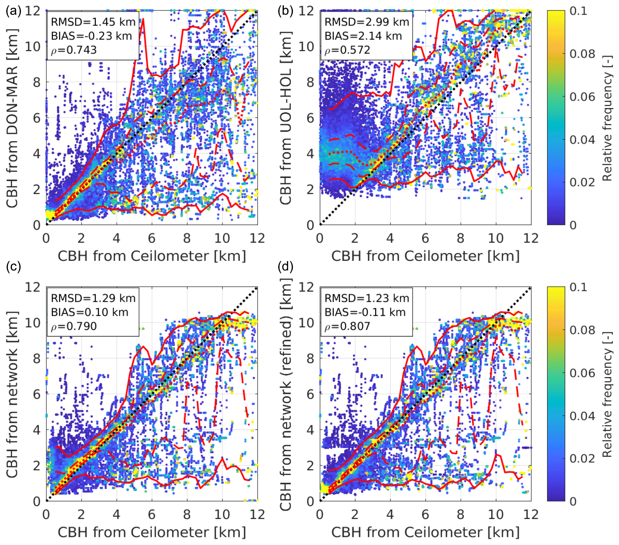
Figure 8 Relative frequency of ASI-based CBH estimation for a given CBH from the ceilometer. An evaluation of two of the ASI pairs, DON-MAR (a) and UOL-HOL (b), with respective camera distances of 0.8 and 5.7 km, and from the ASI network, without (c) and with refinements (d), is shown. The relative frequency in each column adds up to one. Additionally, the median (50 % quantile; red dotted), limits to the interquartile range (IQR; red dashed line) and 5th and 95th percentiles (red solid line), based on floating 1000 m bins of the CBH from ceilometer, are plotted.

4.2.1 ASI pairs

The readings of ASI pair, DON-MAR (Fig. 8; upper row, left), are well aligned with the main diagonal up to a reference CBH of around 4 km. As the reference CBH increases further, the ASI pair increasingly underestimates the CBH, indicated, e.g., by the median. On the contrary, ASI pair, UOL-HOL (Fig. 8; upper row, right), overestimates the CBH massively if the reference CBH decreases below 3 km, whereas, based on the median value, its readings are well aligned with the reference at a larger CBH.

Both ASI pairs exhibit a strong scattering of the measurements, clearly visible from the wide spread of the quartiles, and of the 5th and 95th percentiles. In agreement with the prior finding, DON-MAR is rather precise at a low CBH (≤3 km), whereas UOL-HOL is notably more precise at a greater CBH. The CBH from the ASI pairs often deviates towards a low CBH when the ceilometer measures the CBH in the range 3…12 km. In this range, the 5th percentile of the ASI-based CBH increases only slightly with the reference CBH, and comparably large relative frequencies are found close to the 5th percentile. As discussed in Sect. 4.1, this can result from low cloud layers which are actually present in the ASI pairs' field of view but not at the ceilometer's location.

Qualitatively, the effects seen meet the expectation from the literature (Nouri et al., 2019a; Kuhn et al., 2019; Nguyen and Kleissl, 2014). ASI pairs with a large camera distance are expected to be more accurate when measuring the CBH of high clouds. On the other hand, ASI pairs with large camera distance are expected to be less accurate for the small CBH values and are expected to exhibit a larger minimum CBH below which no physically meaningful readings are received. From the geometric considerations in Sect. 3.1, a minimum CBH of about 0.18×d was expected, where d is the camera distance. For UOL-HOL, a significantly larger minimum CBH of about 2 km is evident. If the reference CBH is smaller than 2 km, the ASI pair yields measurements of the CBH which scatter randomly around a median value of 4 km. This behavior can be explained as the matching procedure failing if patterns are matched which are located at a larger zenith angle than a maximum value. Consequently, random features observed under a zenith angle smaller than the maximum value are often matched erroneously, which yields too large an estimation of the CBH. Similarly, for DON-MAR, a minimum CBH of around 0.3 km is suggested.

Overall, the ASI pairs are characterized by a minimum CBH in the range of 0.32×d. As described above, this suggests that the matching procedure of the ASI pairs almost always fails if the matched windows cover zenith angles larger than 67^∘. Also, for the reference CBH close to this minimum CBH, the ASI pairs yield increased deviations, e.g., below 0.5 and 3 km for DON-MAR and UOL-HOL, respectively.

4.2.2 ASI network

Based on Fig. 8 (bottom row, left), the ASI network without refinements succeeds in combining the preferred properties of ASI pairs with distinct camera distances. The median values of the ASI network are well aligned with the main diagonal for a reference CBH in the range 0.5…10 km. As indicated by the quartiles, the ASI network's precision is similar to that of an ASI pair with a small camera distance, such as DON-MAR, for the reference CBH ≤4 km. For a larger CBH, the network's precision is closer to that of an ASI pair with a large camera distance (such as UOL-HOL).

In the range of reference CBH>10 km, the ASI network constantly returns a CBH of around 10 km. In the studied climate, the reference CBH in this range is comparably rare (see Fig. 4). Therefore, corresponding grid cells of the conditional probability distributions, used by the estimation procedure, were approximated coarsely based on a small number of observations. The ASI network's combination method, using cumulative likelihood, is intended to avoid deviations resulting from these inaccuracies and, thus, to yield a more conservative estimation. However, this approach also suppresses the estimation of the extreme CBH readings, which causes a bias under these conditions. For the analyzed site, deviations found in this range of the CBH are of minor importance.

For very low values of the reference CBH (especially CBH<0.3 km), the ASI network without refinements overestimates the CBH drastically. None of the ASI pairs used has a sufficiently small minimum CBH for this range. We expect that the ASI network's accuracy would be enhanced significantly, especially in this range, if ASI pairs with a camera distance smaller than 0.8 km were added.

To improve the shortcomings connected to conditions with very low clouds (CBH<1 km), the refinements introduced in Sect. 3.3 are applied. As indicated by Fig. 8 (bottom row, right), these refinements significantly improve the ASI network's performance for reference CBH<2 km. In this range, the ASI network behaves, for the most part, like the ASI pairs DON-MAR and MAR-DON. The refinements do not notably affect the statistics for reference CBH≥2 km. Overall, this evaluation indicates that the ASI network performs significantly better than an individual ASI pair, especially if the whole range of the studied reference CBH 0…12 km should be covered. This is also indicated by the performance metrics shown in Fig. 8.

4.3 CBH accuracy under nowcasting conditions

The procedure to estimate the CBH, developed here, will be used as part of a nowcasting system. In this application, it is of special interest to be aware, at any time, of which accuracy can be expected from a specific reading provided by the ASI network. For this purpose, Fig. 9 shows the relative frequency of the CBH measured by the ceilometer given a specific ASI-based estimation of the CBH. In each row, the frequencies add up to one. It should be noted that the performance indicated by this evaluation is more dependent on the local cloud conditions than the one in Sect. 4.2. We analyze the systems which are the best in class, i.e., ASI pair DON-MAR (Fig. 9; left) and the ASI network with refinements (Fig. 9; right). As in the previous section, the plots also include the median (red dotted), limits to the interquartile range (IQR; red dashed line) and the 5th and 95th percentiles (red solid line) based on floating 1000 m bins of the ASI-based CBH.

Figure 9 Relative frequency of the CBH from ceilometer for a given ASI-based CBH estimation. Evaluation of the ASI pair, DON-MAR (a), and of the ASI network with refinements (b). Subplots (a; b) are created analogously to Fig. 8 (a; d). However, relative frequencies add up to one in each row (not column).

Under most conditions included in Fig. 9, the median and interquartile range indicate a good alignment of the CBH estimation from the ASI network and of the CBH from the ceilometer. For the ASI pair DON-MAR, a notable negative bias is indicated if the ASI pair returns a CBH of 9 km or more. Also, if a CBH of more than 4 km is detected, the interquartile range indicates a notably increased precision of the ASI network. The range between the 5th and 95th percentiles is wide for both systems. For a wide range of CBH readings, 5 % of the estimations of the CBH may deviate by more than 4 and 3 km from the ceilometer measurement in the case of the ASI pair and the ASI network, respectively. Still, this range is notably narrower for the ASI network.

Based on Fig. 9, both systems are considered suited for an application in nowcasting at the studied site, while a considerable uncertainty is present. The ASI network provides a notably improved accuracy, particularly in cases when clouds at a CBH>4 km are detected.

4.4 Comparison of the CBH accuracy for a 3-month data set

The statistical evaluations are now restricted to times in which the variability in the CBH is small. More precisely, the standard deviation of the CBH within a window 15 min before and after the analyzed time is required to be less than 30 % of the mean CBH within the same window. As discussed above, the ASI pairs and the ASI network are expected to measure a spatial median CBH, whereas the ceilometer measures the CBH at the point of its installation. This restriction aims to assure a good comparability of both measurements. Furthermore, in this way our results are more comparable to a prior study by Kuhn et al. (2019).

Accuracies of the CBH measurement by ASI pairs and ASI network are analyzed separately for five ranges of the reference CBH defined by the bounds {0, 1, 2, 4, 8 and 12} km. The number of CBH measurements included in this evaluation is given in Table 1 for each of these ranges. The interval bounds are spaced irregularly to correspond better to the distribution of the CBH at the site (see also Fig. 4). Table 1 also shows the number of observations excluded from the validation, as a significant temporal variability in the CBH was detected for these observations. While a significant fraction of the readings is sorted out, the representation of the CBH ranges remains widely comparable to the original data set (see Fig. 2; left). Only the range of the lowest CBH<1000 m is represented by a notably smaller share of the validation data set.

Table 1 Frequency of measurements from the validation data set (30 June to 27 September 2019) per range of cloud base height (CBH) used in the evaluations described in Sect. 4.4 (retained) and frequency of those filtered from the evaluation due to increased variability in the CBH (rejected).

4.4.1 Accuracy of the ASI network and ASI pairs

Figure 10 compares RMSD (left) and bias (right) for the CBH estimated by the ASI network, both with (diamonds) and without the refinements (circles) described in Sect. 3.3, to the one estimated by all ASI pairs (dots). The ASI network with refinements provides the measurements of the CBH that are the most accurate or at least among the most accurate ones for all conditions. In terms of the RMSD, the estimation from the ASI network is the most accurate for the range of $\mathrm{CBH}\in [\mathrm{1},\mathrm{8}[$ km (see Fig. 10; left). For CBH<1 km, it is slightly outperformed by two ASI pairs (DON-MAR and MAR-DON) and for CBH>8 km by two other ASI pairs (UOL-CLO and CLO-UOL). An ASI-network-based measurement of the CBH provides among the smallest bias levels for CBH<8 km (see Fig. 10; right). The magnitude of bias ranges constantly below 100 m. Only for CBH>8 km does the ASI network independent from the applied corrections yield a bias of roughly −1050 m that corresponds to the average bias of all the used ASI pairs for these conditions. This deviation is probably related to situations in which the ASI-based estimation of the CBH recognizes a low cloud layer, whereas the ceilometer also recognizes a high layer when gaps in the low layer appear. Therefore, this deviation is rather related to the different nature of the measurements (spatial median compared to point-wise).

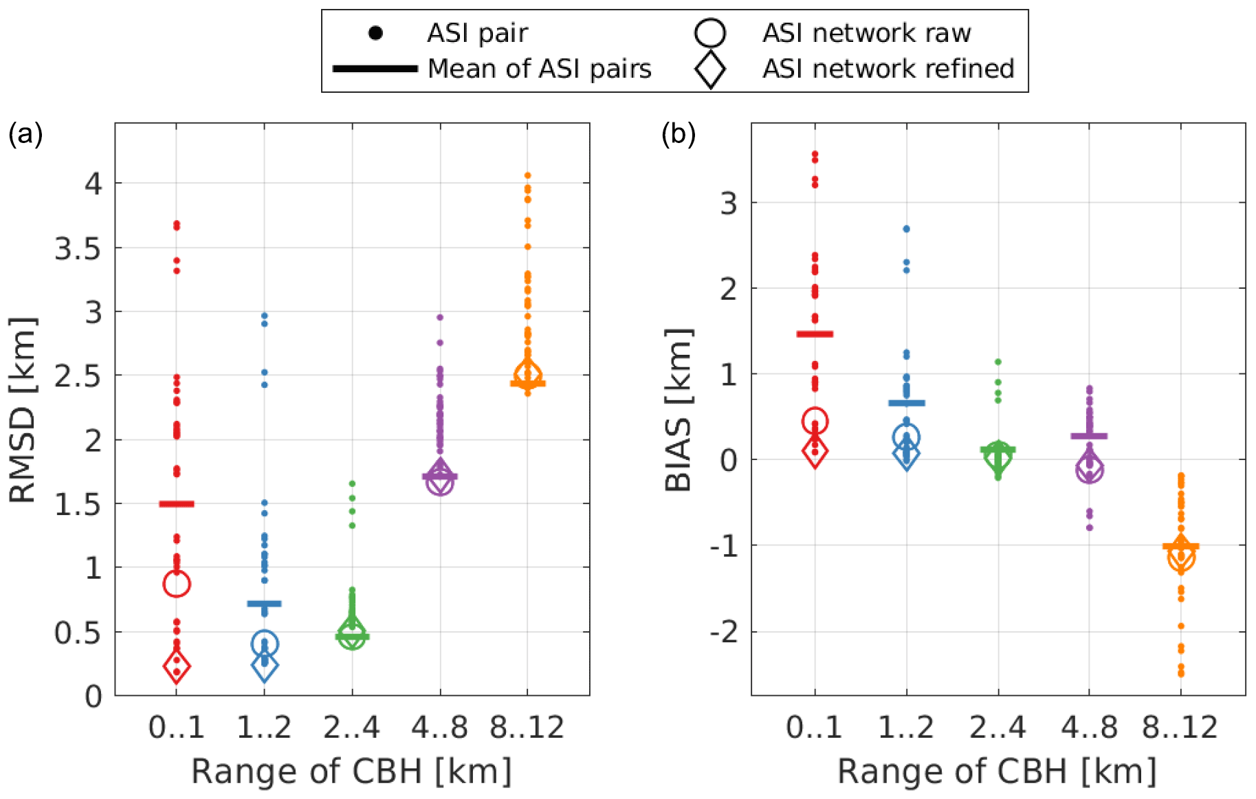
Figure 10 RMSD (a) and bias (b) for five ranges of the CBH received for all individual ASI pairs (dots), for the ASI network without (circles) and with refinements (diamonds) and for a basic average of the CBH measured by all ASI pairs (horizontal line).

The distance between the cameras used by an ASI pair and the reference ceilometer was considered as influencing the accuracy of an ASI pair. However, for the ASI pairs studied, this distance to the validation site is not confirmed as being a significant influence on the received accuracy. This was expected, in part, from the assumption that the ASI pairs measure the median CBH of the most dominant cloud layer in terms of features driven by area and optical thickness.

As shown in Fig. 10 (without the refinements), in the range of CBH<1 km, 12 ASI pairs with a camera distance up to 1.6 km perform better than the ASI network in terms of RMSD and bias. As discussed in Sect. 4.2, in this range of the reference CBH, the ASI network could be improved by ASI pairs with even smaller camera distance. The applied refinements improve the accuracy notably. Figure 10 includes the error metrics received when simply averaging the CBH measurements of all ASI pairs. The ASI network in both variants, i.e., with and without refinements, provides a significantly more accurate estimation of the CBH in terms of RMSD and bias in most ranges of the CBH compared to the simple approach.

The individual ASI pairs and also the ASI network exhibit an RMSD of more than 180 m for all ranges of the CBH. Based on this, we do not expect that the bin size of 100 m chosen for the distributions of conditional probability in Sect. 3.4 is a limiting factor with regard to the accuracy of the ASI-based estimation of the CBH in this study. Meanwhile, the underlying ASI pairs can nowcast 30 s averages of solar irradiance at a spatial resolution of 5 m × 5 m. According to the considerations of Nouri et al. (2019b) and with the Sun elevations occurring at the site, deviations in the CBH may cause deviations in the positions of cloud shadow edges of at least 100 m under favorable conditions for the ASI pairs and also for the ASI network. This deviation is much larger than the spatial resolution of these maps of solar irradiance. For certain applications, e.g., to control solar power plants (Nouri et al., 2020a), it may still be advantageous to provide maps of solar irradiance at a resolution finer than the uncertainty of cloud shadow edge positions, as the statistical properties of spatial variability may still be captured in these maps.

4.4.2 Influence of the camera distance on performance metrics

Lastly, we discuss how camera distance influences the performance metrics of the ASI pairs in different ranges of the CBH and compare these results those of Kuhn et al. (2019), who studied the accuracy of ASI pairs with camera distances in the range of 0.5…2.56 km. Figure 11 provides the RMSD and bias received from the ASI network and ASI pairs and distinguishes the latter by camera distance. Metrics of the ASI network, with refinements, are given by horizontal lines. Kuhn et al. (2019) analyzed the accuracy of the CBH measurement for three ranges of the CBH defined by the limits {0, 3, 8 and 12} km. Overall, in the present study, the magnitudes of RMSD and bias range well below the values found by Kuhn et al. (2019).

Figure 11 RMSD (a) and bias (b) received by 42 ASI pairs utilizing camera distances in the range of 0.8…5.7 km and by the ASI network with refinements (no camera distance applicable) for the period 30 June to 27 September 2019.

For the CBH ranges 0…1 km and 1…2 km, Fig. 11 shows that the bias is very small for ASI pairs with small camera distance. However, beginning at a camera distance of around 1.1 and 2.5 km, respectively, the bias increases linearly with camera distance. Consequently, the same trend is visible for RMSD in these ranges of the CBH. From the analysis in Sect. 4.2, this effect is clearly connected to the minimum CBH specific to an ASI pair's camera distance. While in the study of Kuhn et al. (2019) the lowest CBH range covered 0…3 km, which reduces the influence of the minimum CBH, a qualitatively similar relationship of camera distance and accuracy was found.

For intermediate and large CBHs (4…12 km), the correlation of camera distance and accuracy is less clear; a slight trend seen in RMSD and bias is overlaid by strong scattering. The variation in error metrics found between these systems may indicate further influences of the setup on accuracy – apart from camera distance. On the other hand, the limited set of observations of high clouds may not be sufficiently representative to identify the influence of the camera distance in the presence of other disturbances present in this benchmark, such as low clouds which may be present in spite of the applied filter.

Overall, in the range of the CBH >4 km, increased camera distance slightly improves the accuracy of the CBH estimation. On average, a reduction in RMSD of 500 m is suggested over the interval of studied camera distances. No significant influence is noticed for bias. From Kuhn et al. (2019), the influence of the camera distance on the accuracy was expected to be more significant in this range of the CBH.

Furthermore, the orientation of the ASI pair's axis to the present direction of cloud movement was considered as an influence on accuracy in Kuhn et al. (2019). ASI pairs may measure the CBH more accurately if the ASI pair's axis is aligned with the direction of cloud motion. The direction of the cloud motion was retrieved from ASI UOL, as described in Sect. 3.2, and the data set was filtered to time stamps showing the cloud motion from west to east. Accuracies of ASI pairs with a similar camera distance but a different orientation of the ASI pair's axis were compared. In this comparison, there was no correlation of accuracy, and the alignment of the ASI pair's axis over the direction of cloud motion was recognized.

Based on these findings, we recommend choosing a camera distance of a single ASI pair, which is not part of an ASI network, based on the smallest CBH (CBH_min) that is of interest at a site. This consideration differs from previous studies by Nguyen and Kleissl (2014) and Kuhn et al. (2019) which suggest, based on theoretical and experimental findings respectively, optimizing camera distance for the most frequent or the most relevant CBH. Our experimental results suggest that camera distance of a single ASI pair should, if possible, not be chosen to be larger than 1.4 × CBH_min and in no case should the distance be larger than 3 × CBH_min. For the meteorological conditions studied here, ASI pairs with even smaller camera distances than 0.8 km would be beneficial to cover the range CBH<0.5 km.

5 Conclusions

In this study, a method was presented and benchmarked to estimate the cloud base height (CBH) by a network of all-sky imagers (ASIs). The ASI network-based estimation of the CBH aims to combine the measurements of the CBH from ASI pairs arranged in proximity and organized in a network. Conditional probabilities are modeled from historic CBH measurements received from ASI pairs and a reference ceilometer. These indicate the probability that an ASI pair with specific camera distance would deliver a specific CBH reading if the true CBH actually was in a specific range. In the inference, the ASI network uses this knowledge to calculate the likeliest CBH, given the readings of the CBH from individual ASI pairs. Additionally, accuracy of the CBH measured by 42 independent ASI pairs over a period of 90 d was analyzed. This validation extended prior studies of the analyzed system to the conditions of a Central European climate (Cfb) and to an unprecedented variety of camera alignments and camera distances (0.8…5.7 km).

The influence of camera distance on the accuracy of ASI-based estimation of the CBH was less pronounced than suggested by prior studies. For low clouds (CBH<4 km), small camera distances were found to lead to most accurate measurements. Under these conditions, deviations were found to increase steadily with camera distance as described in the literature. For higher clouds (especially for CBH>8 km) larger camera distances were found to affect received accuracy positively. However, this effect was small compared to the expectation. As a main cause of deviations, a minimum CBH was identified which is specific to each ASI pair. A minimum CBH was found to increase steadily with camera distance of an ASI pair. Below this minimum CBH, ASI pairs were found to return nonphysical and positively biased readings.

When selecting a camera distance for an ASI pair with a stereoscopic estimation of the CBH based on cross-correlation, this study suggests considering the following, depending on the meteorological conditions on-site: ASI pairs with a camera distance of <2 km are accurate only for the CBH up to 4 km. ASI pairs with a camera distance of >3 km are slightly more accurate than ASI pairs with a smaller camera distance for CBH≥4 km but much less accurate for CBH<4 km than ASI pairs with a smaller camera distance. For ASI pairs which are set up at sites with a similar distribution of the CBH as in our study, we recommend including camera distances smaller than 1.8 km. If mostly medium height or high clouds are expected, a greater camera distance is preferable. If possible, multiple setups, also including ASI pairs with small (<0.8 km) and larger camera distances (>1.8 km), are recommended to increase the accuracy for all CBH ranges. However, larger camera distances can help to increase the spatial coverage of an ASI network with a given number of cameras, which is also advantageous. A trade-off between the CBH accuracy and coverage or costs must, hence, be found for ASI networks.

The presented approach for merging the measurements of ASI pairs in an ASI network combined the favored properties of the individual ASI pairs. For all five ranges that were defined for the reference CBH readings by the bin edges $\mathrm{0},\mathrm{1},\mathrm{2},\mathrm{4},\mathrm{8}$ and 12 km, the ASI network provides a measurement that is among the most accurate ones compared to individual ASI pairs in terms of RMSD. Individual ASI pairs slightly outperformed the network but only for single intervals of the CBH. In terms of bias, the same finding was received, except for the range of $\mathrm{CBH}\in [\mathrm{8},\mathrm{12}]$ km. In this CBH range, the ASI network yields an average bias, when compared to the ASI pairs, as all of the ASI pairs are biased for these conditions.

The presented ASI-network-based approach to CBH measurement can be transferred to other sites using the conditional probabilities of the CBH found at the Oldenburg site. Found distributions may then be extended to include more frequent observations of high clouds. Especially regarding its geometric dimensions and spatial coverage, the used setup is suited to airports and large or networked solar power systems.

Based on the present study, the proposed approach to measure the CBH in an ASI network will, in the future, be enhanced by first extending the utilized statistics of the measured CBH with data from other sites at which a combination of ASI pair and ceilometer is available. Such an extended data set will additionally allow us to use more elaborate statistical methods, including neural networks. A procedure for the generation of irradiance nowcasts based on the whole ASI network, utilizing the method to estimate the CBH described here, is under development.

Appendix A: Details on the retrieval of conditional probabilities

A1 Retrieval of raw joint frequency distributions

The CBH from the respective ASI pair and from the ceilometer are processed by a moving median filter with a window of 10 min. The joint frequency distribution of the CBH measured by ceilometer h_Ref and the respective ASI pair h_ASI is computed from these simultaneously acquired time series. That means that the frequency is calculated, with which the tuple of CHB from the ceilometer and ASI pair (h_Ref,h_ASI) is observed in a discrete grid cell defined by the interval $[j\mathrm{\Delta }h,(j+\mathrm{1}\left)\mathrm{\Delta }h\right[$, for h_Ref, and the interval $[k\mathrm{\Delta }h,(k+\mathrm{1}\left)\mathrm{\Delta }h\right[$, for h_ASI, where $j,k\in \mathit{\{}\mathrm{0},\mathrm{1},\mathrm{2},\mathrm{\dots },N-\mathrm{1}\mathit{\}}$, and N is the number of bins used for the CBH in the analysis. A bin size Δh=100 m is chosen in a trade-off between the sources of error. Finer bins will allow us to represent the distributions at higher resolution and will, thus, allow for higher resolved measurements of the CBH in the network. However, the size of the used data set is limited, which makes it difficult to model these distributions at highest resolution. The bin size chosen here is expected to limit the achievable uncertainty of the measurement to a minimum level of 100 m. The joint frequency distributions modeled here are restricted to a maximum CBH of 12 km. This yields N=120.

A2 Filtering operations applied

First, a weighted mean filter is applied between original joint frequency distributions F_l received from all ASI pairs with the camera distance d; this yields F_l,filter 1 the following:

$$\begin{array}{}\text{(A1)}& F_{l,\text{filter 1}}={\displaystyle \frac{{\sum }_m{w}_{l,m}{F}_m}{{\sum }_m{w}_{l,m}}}.\end{array}$$

For the joint frequency distribution F_l of each respective ASI pair l, weights w_l,m are used that include ASI pairs with a similar camera distance. More precisely, a triangular window, based on the difference in the camera distance Δd_l,m of ASI pair m, compared to ASI pair l, is used as defined in the following:

$$\begin{array}{}\text{(A2)}& w_{l,m}=max(\mathrm{0},\mathrm{1}-\mathrm{\Delta }{d}_{l,m}/\mathrm{0.5}\mathrm{km}).\end{array}$$

We decompose each distribution F_l,filter 1 by conditional filters into three separate modes. In the second step, we apply a Gaussian filter g_σ to each mode, with a distinct standard deviation σ_mode of the Gaussian kernel. The subscript, mode, indicates the specific mode for which σ_mode is applied. The first mode is constituted by all outlier observations. Outliers are defined here as grid cells (h_Ref,h_ASI) for which the ASI pair measurement of the CBH h_ASI deviates by more than 1.5 km from the ceilometer reading h_Ref, as follows:

$$\begin{array}{}\text{(A3)}& \begin{array}{rl}& F_{l,\mathrm{outlier}}(h_{\mathrm{Ref}},h_{\mathrm{ASI}})=\\ & \left\{\begin{array}{ll}{F}_{l,\text{filter 1}}(h_{\mathrm{Ref}},h_{\mathrm{ASI}}),& \left|h_{\mathrm{ASI}}-h_{\mathrm{Ref}}\right|>\mathrm{1.5}\mathrm{km}\\ \mathrm{0},& \text{else.}\end{array}\right.\end{array}\end{array}$$

Such outliers will contain a large random component. We expect that, in a reproduction of the experiment, a similar number of outliers will be received, while the joint frequency found for a single grid cell (h_Ref,h_ASI) may vary significantly. Therefore, the strongest filter is applied to this mode using σ_outlier=1 km.

The second mode is constituted by grid cells that are not part of the first mode and feature a joint frequency which is less than the average over all grid cells of the joint frequency distribution, as follows:

$$\begin{array}{}\text{(A4)}& \begin{array}{rl}& F_{l,\mathrm{inconfident}}(h_{\mathrm{Ref}},h_{\mathrm{ASI}})=\\ & \left\{\begin{array}{ll}{F}_{l,\text{filter 1}}(h_{\mathrm{Ref}},h_{\mathrm{ASI}}),& \left|h_{\mathrm{ASI}}-h_{\mathrm{Ref}}\right|\le \mathrm{1.5}\mathrm{km}\\ & \wedge F_{l,\text{filter 1}}(h_{\mathrm{Ref}},h_{\mathrm{ASI}})<\text{mean}\left(F_{l,\text{filter 1}}\right)\\ \mathrm{0},& \text{else.}\end{array}\right.\end{array}\end{array}$$

The comparably small number of observations in these grid cells is expected to cause an increased uncertainty of the estimated joint frequencies. For this mode, σ_inconfident=0.5 km is applied.

The third mode $F_{l,\mathrm{confident}}(h_{\mathrm{Ref}},h_{\mathrm{ASI}})$ makes up the complement of the first and second mode. It contains grid cells that are observed with an, at least, average joint frequency and which are not classified as outliers, as follows:

$$\begin{array}{}\text{(A5)}& \begin{array}{rl}& F_{l,\mathrm{confident}}(h_{\mathrm{Ref}},h_{\mathrm{ASI}})=\\ & \left\{\begin{array}{ll}{F}_{l,\text{filter 1}}(h_{\mathrm{Ref}},h_{\mathrm{ASI}}),& \left|h_{\mathrm{ASI}}-h_{\mathrm{Ref}}\right|\le \mathrm{1.5}\mathrm{km}\\ & \wedge F_{l,\text{filter 1}}(h_{\mathrm{Ref}},h_{\mathrm{ASI}})\ge \text{mean}\left(F_{l,\text{filter 1}}\right)\\ \mathrm{0},& \text{else.}\end{array}\right.\end{array}\end{array}$$

Joint frequencies in these grid cells are considered to have a comparably high accuracy. To avoid a loss of precision and, ultimately, a loss of accuracy in the estimation of the CBH, a small value of σ_confident=0.1 km is used. The three filtered modes g_σ are summed to receive the smoothed joint frequency distribution as follows:

$$\begin{array}{}\text{(A6)}& \begin{array}{rl}{F}_{l,\text{filter 2}}& =g_{{\mathit{\sigma }}_{\mathrm{outlier}}}\left(F_{l,\mathrm{outlier}}\right)\\ & +g_{{\mathit{\sigma }}_{\mathrm{inconfident}}}\left(F_{l,\mathrm{inconfident}}\right)\\ & +g_{{\mathit{\sigma }}_{\mathrm{confident}}}\left(F_{l,\mathrm{confident}}\right).\end{array}\end{array}$$

For all grid cells, the joint frequency is increased to a minimum value of 0.5 to avoid underestimations of the joint frequency. This value is chosen to be half of the joint frequency associated with a single actual observation in a grid cell.

Each joint frequency distribution is normalized with the sum of all joint frequency grid cells. In this way, a probability mass function P(h_Ref,h_ASI) (also known as discrete density function) to measure a certain CBH with the respective ASI pair and to coincidentally measure a certain CBH with the ceilometer is yielded. The conditional probability P(h_ASI | h_Ref) of receiving a certain CBH reading from an ASI pair, given that the ceilometer measures some certain CBH, is calculated by dividing the respective probability mass function by the marginal distribution of the CBH measured by the ceilometer. The latter distribution gives the probability of receiving the CBH from the ceilometer within a certain bin h_Ref, regardless of which CBH reading is simultaneously received from an ASI pair. The distribution can be derived from any of the probability mass functions by summing all the grid cells of the probability mass function which correspond to the respective bin h_Ref of the CBH measured by the ceilometer.

A3 Representation of intervals of camera distance

The inference procedure represents each range i of the camera distance bounded by the limits $\mathit{\{}\mathrm{0.5},\mathrm{1},\mathrm{1.5},\mathrm{\dots },\mathrm{6}\mathit{\}}$ km and by a single distribution of conditional probability. For each range of camera distance, the distribution of conditional probability, which corresponds to the camera distance closest to the center of this range, is selected. For example, for the range i=2 representing camera distances 1…1.5 km, the center of the range would be 1.25 km. For the camera distances 1.081, 1.247 and 1.352 km, conditional probabilities have been modeled. Consequently, for this range of camera distance, the distribution of conditional probability corresponding to the camera distance 1.247 km is used.

Appendix B: Comparison of the CBH time series

B1 Estimation of the CBH during a clear sky period

Figure B1 provides a detailed view of the CBH measured by ASI pairs, by the ASI network and by the ceilometer during a mostly clear period on 2 September 2019. The period is discussed in Sect. 4.1.

B2 Comparison of the CBH measurements for another exemplary day

Figure B2 shows the CBH on 6 August 2019, again measured by the ceilometer, by all available ASI pairs and by the ASI network. This day, similar to 2 September 2019, as discussed previously, includes multilayer conditions, with high layers overlain by low layers, resulting in similar observations. In the morning and evening, high cloud layers are dominant. The CBH of these varies in the range of 7…11 km according to the ceilometer. The range of the CBH from the ASI pairs reflects this spread. Still, it is not obvious which of the ASI-pair-based observations would be the most appropriate. From the ASI network, a rather steady CBH estimation results, which, most of the time, reflects the dominant CBH layer as recognized by the ceilometer. The combined estimation misses physically meaningful variations in the CBH, typically towards higher values recognized by the ceilometer. Also for this day, the time series of the CBH and corresponding ASI images were compared. Again large underestimations of the CBH by the ASI network (at 05:30, 08:15, 10:00, 12:30, and 16:00) were traced back to the ASI-based estimations responding stronger to lower optically denser low cloud layers which pass the vicinity of the urban area (compare Fig. B3).

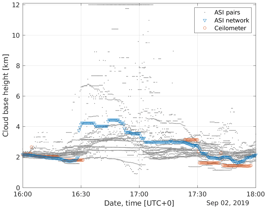
Figure B1 Detailed view of the CBH measured by ASI pairs (gray dots), by the ASI network (blue triangles) and ceilometer (red circles) during a period with low sky coverage. Around 17:00, approaching clouds are viewed close to the horizon by all ASIs.

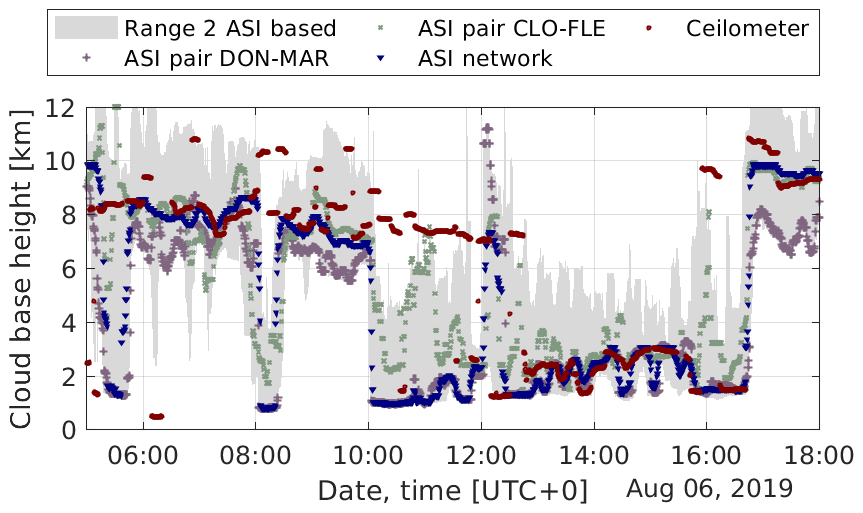
Figure B2 Time series of cloud base height for an exemplary day (6 August 2019) measured by 42 ASI pairs (gray filled), by two exemplary ASI pairs, DON-MAR and CLO-FLE with respective camera distances 0.8 and 4.2 km, by the ASI network with refinements and by a ceilometer in the urban area of Oldenburg.

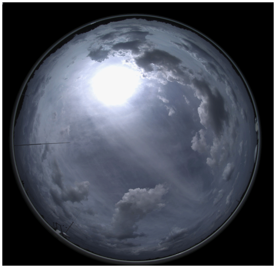
Figure B3 Sky image taken by ASI UOL, representing a multi-cloud-layer situation on 6 August 2019 12:35.