Real-time UV index retrieval in Europe using Earth observation-based techniques: system description and quality assessment

This study introduces an Earth observation (EO)-based system which is capable of operationally estimating and continuously monitoring the ultraviolet index (UVI) in Europe. UVIOS (i.e., UV-Index Operating System) exploits a synergy of radiative transfer models with high-performance computing and EO data from satellites (Meteosat Second Generation and Meteorological Operational Satellite-B) and retrieval processes (Tropospheric Emission Monitoring Internet Service, Copernicus Atmosphere Monitoring Service and the Global Land Service). It provides a near-real-time nowcasting and short-term forecasting service for UV radiation over Europe. The main atmospheric inputs for the UVI simulations include ozone, clouds and aerosols, while the impacts of ground elevation and surface albedo are also taken into account. The UVIOS output is the UVI at high spatial and temporal resolution (5 km and 15 min, respectively) for Europe (i.e., 1.5 million pixels) in real time. The UVI is empirically related to biologically important UV dose rates, and the reliability of this EO-based solution was verified against ground-based measurements from 17 stations across Europe. Stations are equipped with spectral, broadband or multi-filter instruments and cover a range of topographic and atmospheric conditions. A period of over 1 year of forecasted 15 min retrievals under all-sky conditions was compared with the ground-based measurements. UVIOS forecasts were within ±0.5 of the measured UVI for at least 70 % of the data compared at all stations. For clear-sky conditions the agreement was better than 0.5 UVI for 80 % of the data. A sensitivity analysis of EO inputs and UVIOS outputs was performed in order to quantify the level of uncertainty in the derived products and to identify the covariance between the accuracy of the output and the spatial and temporal resolution and the quality of the inputs. Overall, UVIOS slightly overestimated the UVI due to observational uncertainties in inputs of cloud and aerosol. This service will hopefully contribute to EO capabilities and will assist the provision of operational early warning systems that will help raise awareness among European Union citizens of the health implications of high UVI doses.

1 Introduction

Human exposure to ultraviolet (UV) radiation (< 400 nm) has both beneficial and harmful effects (Andrady et al., 2015; Juzeniene et al., 2011; Lucas et al., 2006). Overexposure to UV radiation (UVR) has a number of implications, such as the acute response of erythema, the risk of skin cancer and a number of eye diseases (snow blindness, cataract). Nevertheless, exposure to solar UVB radiation (290–315 nm) is the main mechanism for the synthesis of vitamin D in human skin (Holick, 2002; Webb and Engelsen, 2008; Webb et al., 2011). Low levels of vitamin D are associated with depression of the immune system, and there is evidence that it is linked to a number of medical implications (Lucas et al., 2015).

The UV index was introduced by the WHO/WMO in 1994 (WMO, 1995) as a simple method of informing the general public about the erythema effective (sun-burning) UV. It is a unitless, scaled version of erythemally weighted UV determined by multiplying the erythema weighted irradiance (in W m⁻²) by 40 m² W⁻¹ (Fioletov et al., 2010; Vanicek et al., 2000; WHO, 2002). The response of UV radiation to climatic changes is of great concern (Bais et al., 2019, 2018; McKenzie et al., 2011). According to the latest work of Bais et al. (2019), greater values of UV are expected by the end of the 21st century, relative to the present decade, at low latitudes, while at higher latitudes UV will decrease, but these projections are associated with high uncertainty (up to 30 %).

There are many factors affecting UV irradiance reaching Earth's surface (Kerr and Fioletov, 2008). The dependence of UV irradiance on astronomical and geometrical parameters is generally well understood, and in many cases the changes are periodical (e.g., Blumthaler et al., 1997; Gröbner et al., 2017; Larkin et al., 2000; Seckmeyer et al., 2008). Atmospheric gases play a crucial role in attenuating UV irradiance; specifically, NO₂ is a major absorber in the UV (e.g., Cede et al., 2006), while O₃ is the main absorber at lower (UVB) wavelengths. Other gases that have significant absorption in the UV include SO₂ (Fioletov et al., 1998) and HCHO (Gratien et al., 2007), but their – usually – smaller atmospheric abundances result in minor effects on incoming UV (with major exceptions such as volcanic incidents). Aerosols are another important parameter controlling UV irradiance levels at the surface (e.g., Kazadzis et al., 2009b). Aerosol optical depth (AOD) that quantifies the attenuation of the direct solar beam by aerosols is a parameter varying with wavelength. Single scattering albedo (SSA), which determines the scattering ratio to total extinction, is also a spectrally variant parameter. Several recent studies based on surface UV irradiance measurements or calculations reveal the enhanced absorption by aerosols in the UV relative to the visible spectral range. Finally, a number of studies have highlighted the importance of using representative SSA in the UV spectral region instead of interpolating SSA at visible wavelengths to the UV or directly using SSA at visible wavelengths, options that systematically overestimate UV irradiance (Corr et al., 2009; Fountoulakis et al., 2019; Kazadzis et al., 2016; Mok et al., 2018; Raptis et al., 2018).

All the aforementioned parameters are particularly important under cloud-free conditions. The cloudy sky complicates the propagation of solar radiation, predominantly in the troposphere, through multiple cloud–radiation interactions. Nonetheless, UVR is less affected than the total solar radiation by clouds (e.g., Badosa et al., 2014). Bais et al. (1993) quantified that for the city of Thessaloniki the change from 0 to 8 oktas for cloud coverage corresponds to 80 % reduction in the UVR and pointed out that there is very low wavelength dependence of UVR attenuation by cloud cover. Although the transmittance of clouds does not vary significantly with wavelength, some studies (Mayer et al., 1998; Seckmeyer et al., 1996) have found that the diffuse component of the surface UVR is affected by clouds in a spectrally dependent way due to more efficient scattering and absorption of shorter UV wavelengths in the case of large air masses. In cases of partially cloudy sky but unobscured Sun, UVR tends to be higher than in clear-sky conditions (e.g., Badosa et al., 2014), as is the case for total solar radiation. For short timescale analysis the variability of UVR introduced by clouds should be considered.

Solar UV irradiance at the surface increases with increasing surface albedo. This increment affects the UV radiant exposure, which becomes crucial for outdoor human activities (Schmalwieser and Siani, 2018; Schmalwieser, 2020; Siani et al., 2008). Measurements and computations of effective surface albedo for heterogeneous surfaces reveal its strong spectral dependence, with snow-covered surfaces having significantly higher values of albedo for short wavelengths compared to total solar radiation (Blumthaler and Ambach, 1988; Kreuter et al., 2014). Stronger enhancement of the UV relative to visible radiation over highly reflective surfaces is also due to the more effective multiple scattering of shorter wavelengths in the atmosphere.

Any systematic changes in any of the parameters described in previous paragraphs have the potential to lead to changes for UVR. These changes vary significantly throughout the globe and are attributed to different possible drivers (Bernhard and Stierle, 2020; Fountoulakis et al., 2018; McKenzie et al., 2019). Fountoulakis et al. (2020a) give a review of recent publications concerning UV trends since the 1990s and associated factors, summarizing these as positive trends for southern and central Europe and negative trends at higher latitudes and recognizing the important role of aerosols and cloud coverage for these trends. Chubarova et al. (2020) found a long-term increase of 3 % per decade in UV in northern Eurasia for the 1979–2015 period. For the northern mid-latitudes Zerefos et al. (2012) showed that the long-term (1995–2006) positive trend in total ozone was not enough to compensate for, let alone reverse, the UVB increase attributed to tropospheric aerosol decline (brightening effect). Since 2007, a slowdown or even a possible turning point in the positive UVB trend has been detected, which has been attributed to the continued upward trend in total ozone overwhelming the aerosol effect (Zerefos et al., 2012). By contrast, the long-term variability of UVB irradiance over northern high latitudes was determined by ozone and not by aerosol trends, as shown by Eleftheratos et al. (2015), who found a statistically significant negative trend of −3.9 % per decade for the UVB irradiance during the time period 1999–2011, in agreement with a statistically significant increase in spaceborne-measured total ozone by about 1.5 % per decade (ozone recovery) for the same area.

The continuous monitoring of the UV index is currently performed by about 160 stations from 25 countries around Europe (Schmalwieser et al., 2017), with all monitoring instruments having the potential to provide other effective doses such as the effective dose for the production of vitamin D in human skin (e.g., Fioletov et al., 2009).

There are three types of instruments for UV irradiance measurements: those measuring the integral of UV irradiance (broadband sensors) tailored to a specific response, narrow-band instruments such as filter radiometers with coarse spectral resolution, and instruments performing high-resolution spectral measurements – the most versatile but most challenging and least robust instruments. Concerning the current UV monitoring measurement accuracy, the European reference UV spectroradiometer (QASUME) is a traveling instrument which provides a common standard through inter-comparison on-site (Gröbner et al., 2005; Hülsen et al., 2016). During the period 2000–2005 QASUME visited 27 spectroradiometer sites. Out of the 27 instruments, 13 showed deviations of less than 4 % relative to the QASUME reference spectroradiometer in the UVB (for 15 instruments in the UVA) for solar zenith angles below 75^∘. The expanded relative uncertainty (coverage factor k = 2) of solar UV irradiance measurements by QASUME, for solar zenith angle (SZA) smaller than 75^∘ and wavelengths longer than 310 nm, was 4.6 % in 2002–2014 (Gröbner and Sperfeld, 2005) and has been 2 % since 2014 (Hülsen et al., 2016). For broadband instruments, the current instrument uncertainties are summarized in Hülsen et al. (2020, 2008). In 2017, 75 broadband instruments measuring the UV index and the UVB or/and the UVA irradiance participated in the solar UV broadband radiometer comparison in Davos, Switzerland. Using the instrument/user calibration factors, the differences between the data sets by the broadband instruments and the reference (QASUME) data set were within ±5 % for 32 (43 %) of the instrument data sets, ±10 % for 48 (64 %) and exceeded ±10 % for 27 (35 %).

Although ground-based monitoring of solar UVR is more accurate than satellite retrievals, ground-based stations are sparse, and the only way for continuous monitoring of the UVR on a global scale is through satellites. In recent decades instruments onboard satellites have provided the necessary data for estimates of UV irradiance reaching the Earth's surface on a global scale (Herman, 2010), and hence satellite-derived UVR climatological studies have been conducted (Vitt et al., 2020; Verdebout, 2000). The satellite UV irradiance record started with the Total Ozone Mapping Spectrometer (TOMS) onboard Nimbus-7 in 1978 and continued with the Ozone Monitoring Instrument (OMI) onboard NASA's satellite EOS-Aura. The OMI retrieval algorithm for surface UVR estimates was based on the experience gained from TOMS (Levelt et al., 2018, 2006). The early surface UVR retrieval algorithms from satellite data did not account for the enhanced aerosol absorption in the UV spectral range, resulting in overestimated values (Krotkov et al., 1998). A lot of scientific effort has been put into correcting the products (Arola et al., 2009). The TROPOspheric Monitoring Instrument (TROPOMI) onboard Sentinel-5 Precursor (Lindfors et al., 2018) is the current satellite instrument that provides the surface UVR product on a daily basis with global coverage, including 36 UVR parameters. As the aforementioned instruments were installed onboard polar-orbiting satellites, providing global spatial coverage, the temporal resolution of the data is daily since there are only one or two overpasses per day for every point. Geostationary satellites provide continuous (in time) measurements over wide areas. The geostationary meteorological satellites Meteosat monitor the full Earth disk including Europe, and their frequent data acquisition of rapidly changing parameters, e.g., cloud, is essential for estimating daily UV doses (Verdebout, 2000).

Comparison of OMI surface UV irradiance estimates with ground-based measurements for Thessaloniki, Greece, showed that OMI irradiances overestimate surface observations for UVB wavelengths by between ∼ 1.5 % and 13.5 %, in contrast to underestimated satellite values for UVA wavelengths (Zempila et al., 2016). Results from the validation of the TROPOMI surface UV radiation product showed that most of the satellite data agreed within ±10 % with ground-based measurements for snow-free surfaces (Lakkala et al., 2020). Larger differences between satellite data and ground-based measurements were observed for sites with non-homogeneous topography and non-homogeneous surface albedo conditions. The differences between ground-based and satellite UVR data are mostly due to uncertainties in the input parameters to the satellite algorithm used to retrieve the UV irradiance at the surface. Based on a recent study of Garane et al. (2019), a mean bias of 0 %–1.5 % and a mean standard deviation of 2.5 %–4.5 % were found for the relative difference between the TROPOMI total ozone column (TOC) product and ground-based quality-assured Brewer and Dobson TOC measurements.

In this study we introduce a novel UV-Index Operating System, called UVIOS, which is able to efficiently combine information on geophysical input parameters from different modeled and satellite-based data sources in order to provide for the European region the best possible UV index (UVI) estimates operationally and in real time. The reliability of the UVIOS input and output parameters was tested for the year 2017 against ground-based measurements, and an analytical sensitivity analysis was performed in order to quantify the uncertainties and to provide information about the limitations and about the optimum operating conditions of the proposed system.

In Sect. 2 we describe UVIOS and the input data sources, while Sect. 3 presents the ground-based measurements used as well as the evaluation methodology. Section 4 analyzes the results in terms of model performance and factors that affect the UVIOS retrievals and the overall accuracy. Finally, Sect. 5 summarizes the findings and the main conclusions of this study and provides a brief description of the future plans with this system.

2 UVIOS

2.1 System description

UVIOS is a novel model that uses real-time and forecasted atmospheric inputs based on satellite retrievals and modeling techniques and databases in order to nowcast and forecast the UVI with a spatial resolution of 5 km and a temporal resolution of 15 min. The UVIOS calculation scheme is based on the libRadtran library of radiative transfer models (RTMs) (Mayer and Kylling, 2005) within which all the available inputs (i.e., solar elevation, cloud and aerosol optical properties, ozone) can be integrated in real time into the radiative transfer code and calculate the UVI for each pixel. Afterwards, post-processing correction for the elevation of each location and the surface albedo is also performed. In order to be able to simulate the UVI for 1.5 million pixels in real time, we use pre-determined spectral solar irradiance LUTs based on the Libradtran RTM in combination with high-performance computing (HPC) architectures that speed up the process of choosing and interpolating/extrapolating the right combinations from the LUTs (Kosmopoulos et al., 2018; Taylor et al., 2016). The result is the retrieval of the UVI for 1.5 million pixels covering the European domain in less than 5 min after receiving all necessary input parameters.

Table 1 UVIOS model input parameters.

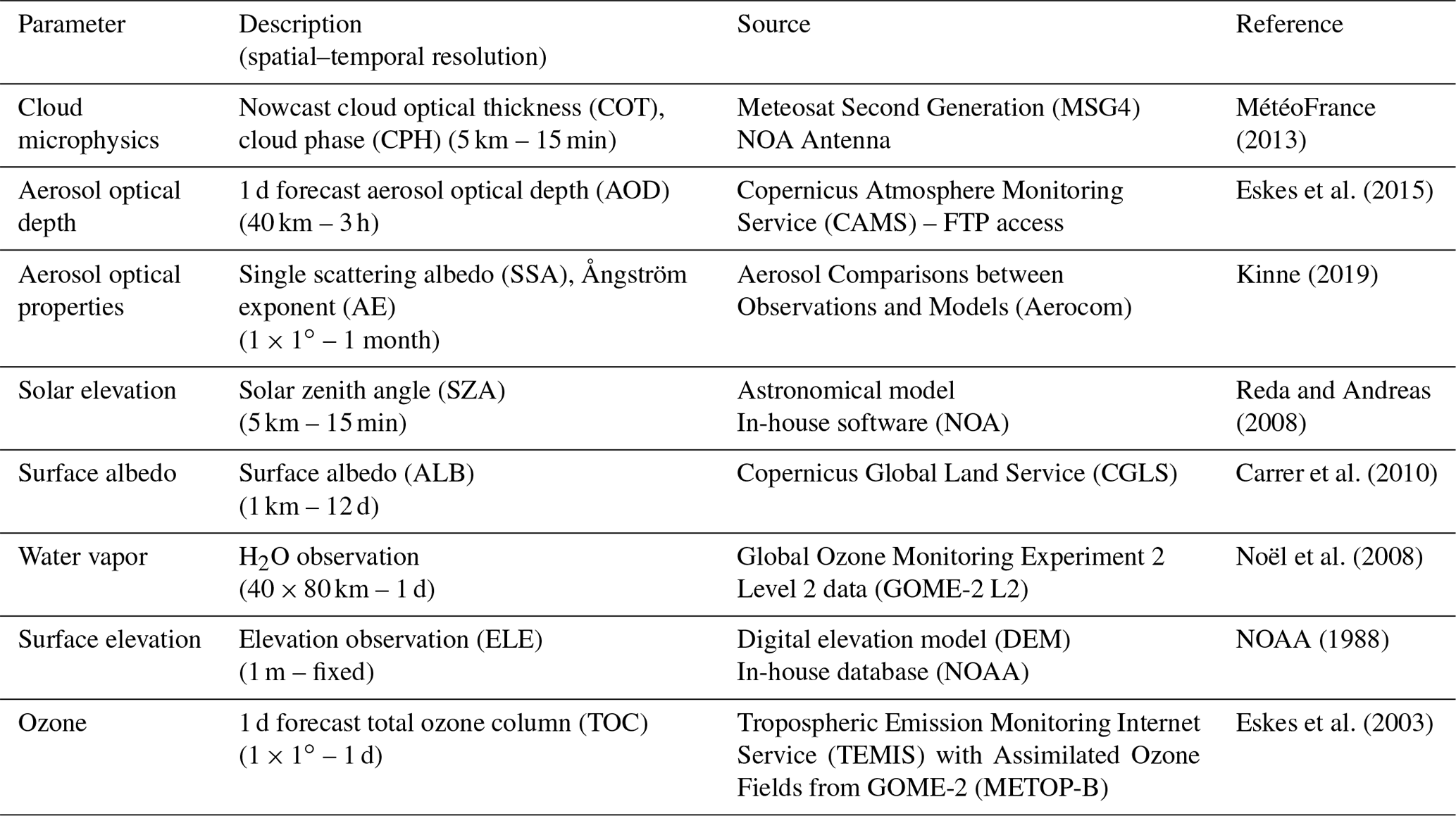
As mentioned, the UVIOS architecture does not include a clear-sky model and the subsequent calculation of individual sources of UV attenuation, but instead it directly uses the following parameters: SZA, AOD and other aerosol optical properties, e.g., SSA, asymmetry parameter, and Ångström exponent (AE), the TOC, the cloud optical thickness (COT), as well as the surface elevation (ELE) and the surface albedo (ALB) as RTM inputs. Table 1 presents the Earth observation (EO) data used as inputs for the UVI real-time simulations and their description and sources. The Meteosat Second Generation (MSG) cloud microphysics includes the nowcasted COT at 550 nm and cloud phase (CPH) obtained at spatial and temporal resolutions of 5 km (average, depending on latitude) and 15 min, respectively. Typical values of other cloud properties (e.g., cloud height, cloud thickness) have been assumed based on the cloud type (information which is also available from MSG) (for more detailed information, see Taylor et al., 2016). The 1 d forecast Copernicus Atmospheric Monitoring Service (CAMS) AOD at 550 nm is obtained at spatial and temporal resolutions of 40 km and 3 h, respectively, and the monthly aerosol optical properties obtained from Aerocom (Kinne, 2019) include asymmetry parameter, SSA and AE at 1^∘ × 1^∘ (latitude × longitude) spatial resolution. Solar elevation is taken from the astronomical model (NREL) (5 km – 15 min) (Reda and Andreas, 2008) and climatological ALB is retrieved from the Copernicus Global Land Service (CGLS) (1 km – 12 d) (Carrer et al., 2010). ELE is obtained from the digital elevation model (DEM) of NOAA (NOAA, 1988). The Tropospheric Emission Monitoring Internet Service (TEMIS) 1 d forecast of total ozone column (TOC) is at a spatial resolution of 1^∘ × 1^∘ – 1 d with assimilated ozone fields from the Global Ozone Monitoring Experiment (GOME-2) (METOP-B) (Eskes et al., 2003). We have to mention also here that the selection of the RTM inputs has been decided based on their real-time availability.

2.2 Real-time processing concept

The LUT approach, despite its large size (almost 2.5 million spectral RTM simulations for clear- and all-sky conditions) (Kosmopoulos et al., 2018), still provides estimates at discrete input parameter values. To overcome this mathematical issue, we performed a multi-parametric interpolation technique to correct the input–output parameter intervals. This solution is computationally more costly than a continuous function-approximation model, i.e., a neural network (NN) model (Kosmopoulos et al., 2018), but the accuracy improvement is significant. Indicatively, using a test set of 1 million RTM simulations for UVI from the developed LUT, we applied the NN developed in Kosmopoulos et al. (2018) and found a mean execution time of around 144 s followed by a mean absolute error (MAE) of 0.0321, while by using the proposed UVIOS multi-parametric interpolation exploiting the HPC and distributed computing benefits, we found for the same test set an execution time of 295 s with a MAE of 0.0001. The inclusion of many parameters (in this study we incorporated eight, i.e., AOD, SZA, TOC, COT, ELE, ALB, AE, and SSA) with small step sizes dramatically increased the LUT size, followed by high computing requirements for the multi-parametric interpolation/extrapolation procedures.

For the UVIOS simulations performed in this study, a 32-core UNIX server was used equipped with 256 GB of RAM and 12 TB of a storage system working in a RAID10 architecture. The combination of the HPC with the analytical LUTs, which were developed by using the libRadtran RTM, allows a high-speed multi-parametric interpolation and polynomial reconstruction (Gal, 1986) to increase accuracy between the LUT records following a mathematical equation relating the UVIOS outputs to the EO inputs.

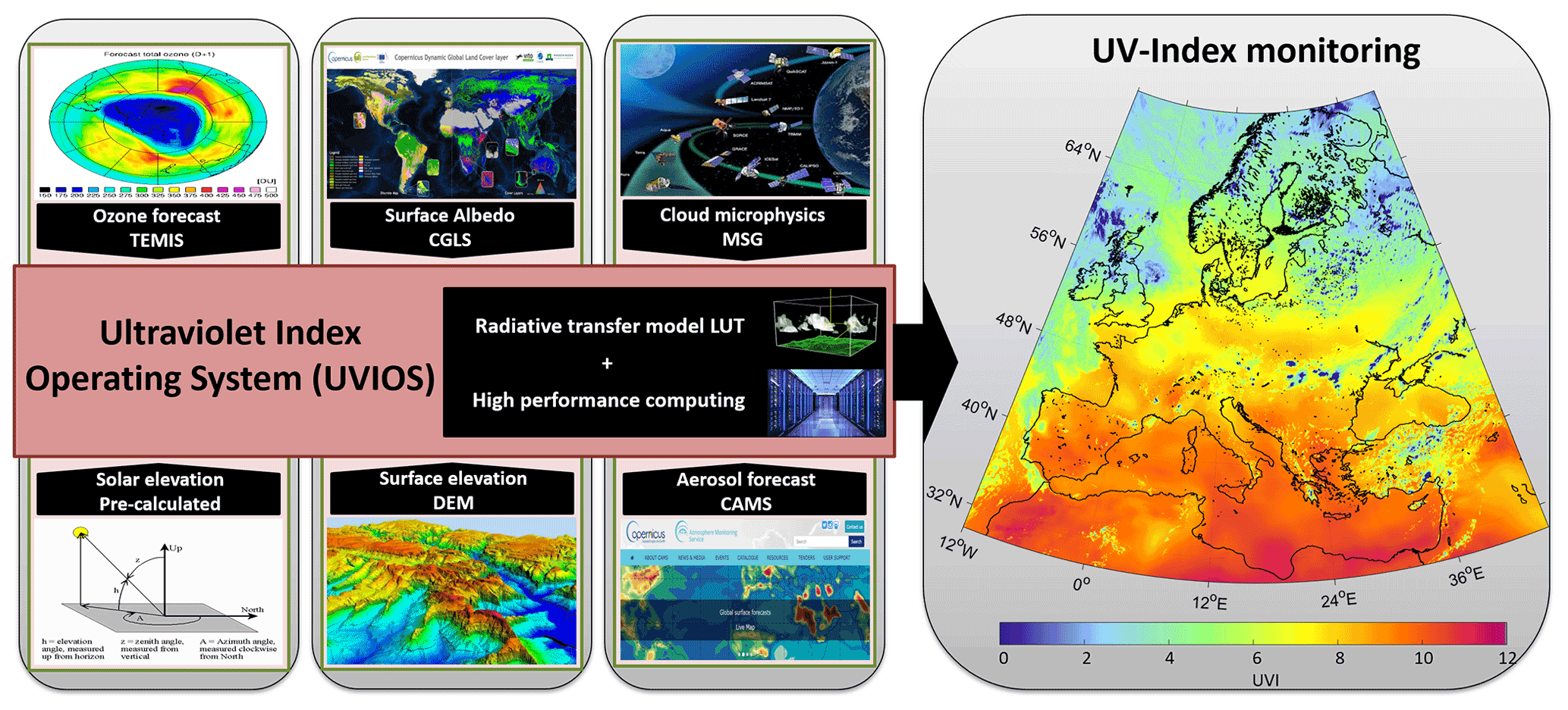
Figure 1 Flowchart illustration of the UVIOS modeling technique scheme. The pre-calculated effects of solar and surface elevation and albedo followed by the aerosol and ozone forecasts and the real-time cloud observations to the UVIOS solver result in the spectrally weighted output of UVI for the European region.

An example of the UVIOS input–output data is presented in Fig. 1 through a flowchart illustration of the modeling technique scheme. The inputs, including the solar and surface elevation, albedo, aerosol, ozone forecasts and cloud observations as described in Table 1 are fed to the real-time solver that results in spectrally weighted output of UVI for the European region. Figure 2 shows the memory usage and error statistics for a range of different LUT sizes. The LUT error decreases as the LUT size increases, regardless of the function being approximated. The LUT sizes in Fig. 2 fit into the cache in our HPC environment; thus, performance in terms of processing speed and overall output accuracy vary only slightly between the table sizes shown. In our case, UVIOS shows that LUT transformation can provide a significant performance increase without incurring an unreasonable amount of error, provided there is sufficient memory available. We note that the cache size is a critical factor for LUT performance, while under a HPC environment practically there is no limit. Such techniques can be implemented in hardware with distributed computing that operates in parallel to provide optimum performance.

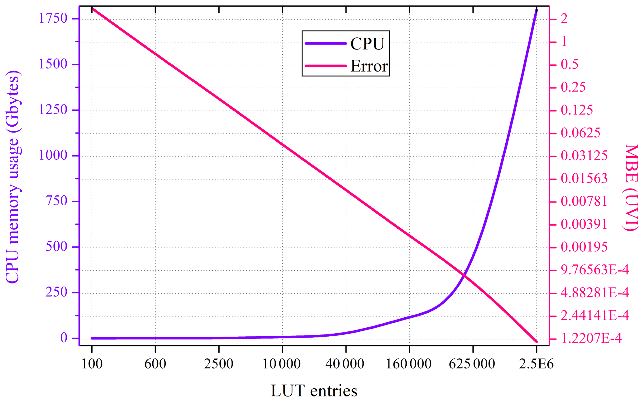
Figure 2 UVIOS memory usage and error statistics in terms of mean bias error (MBE) for a range of different LUT sizes.

Since UVIOS can produce massive UVI outputs of the order of 1.5 million simulations in less than 5 min following the proposed simulation and computing architecture, this means that it can be used for both operational applications and real-time estimations. The exact use of UVIOS depends only on the available input data sources. For this study both nowcasts (clouds) and forecasts (ozone, aerosol) were used as inputs to the system. The nowcasts represent the continuous monitoring dimension (i.e., what is happening now) in terms of cloud microphysics data every 15 min retrieved in real time by the geostationary satellite MSG. The forecasts represent the future estimations (day ahead in our study) of aerosol optical properties and total ozone column based on deterministic approaches (European Centre for Medium-Range Weather Forecasts – ECMWF) and assimilated satellite data for better accuracy. As a result, UVIOS under cloudless conditions operates as a forecast system since it uses forecasted inputs and provides the clear-sky UVI forecasts operationally. By adding the nowcast cloud information as input to UVIOS (i.e., all-sky conditions), the whole procedure will follow the time steps of MSG cloud microphysics data collocated and synchronized with the forecast data. So, following the proposed operation method of this study, UVIOS can be used as a UVI forecast system for cloudless conditions or as a UVI nowcast system for all-sky conditions.

2.3 Input data description

The COT data from Meteosat was used, whose retrieval algorithm is based on 0.6 and 1.6 µm channel radiances of Meteosat's Spinning Enhanced Visible and InfraRed Imager (SEVIRI). MSG products have been described in Derrien and Le Gléau (2005) and the MétéoFrance (2013) technical report. The COT impact uncertainty in UVI deals with the MSG COT reliability and accuracy and hence introduces errors into the UVIOS simulations (Derrien and Le Gléau, 2005; Pfeifroth et al., 2016). In addition, comparison principles of (point) station UVI measurements with a 5 km MSG COT matrix are possibly responsible for at least part of the observed deviations (e.g., Kazadzis et al., 2009a). For instance, when a MSG pixel is partly cloudy, the ground measurements of UVI could fluctuate by more than 100 %, depending on whether the Sun is visible or whether clouds attenuate the direct component of the solar irradiance. The result is that in cases of partly covered MSG pixels and in the absence of clouds between the ground measurement and the Sun, the ground truth UVI would be much higher than the UVIOS one. Of course, the presence of small clouds which have not been identified by MSG and cover (part of) the Sun disk is plausible as well, consequently causing an overestimation of the modeled UVI (Koren et al., 2007). Furthermore, sensors onboard geostationary satellites suffer from the parallax error, which contributes to the spatial errors of the images and the overall uncertainty of the products (Bieliński, 2020; Henken et al., 2011). The error depends on the altitude of the cloud and the viewing angle (parallax errors are more significant for high viewing angles).

UVIOS calculations at high solar zenith angles (> 70^∘) are retrieved assuming cloudless skies since the MSG COT product is not available in these conditions, facing reliability issues (Kato and Marshak, 2009). This has an effect on the quality of the UVIOS overall performance at high solar zenith angles, where there is no cloud information as input to the model in order to quantify the consequent impact on UVI. However, such measurements under high solar zenith angles are accompanied by very low UVI levels (< 1), both in the performed RTM simulations and in the ground-based measurements. This inconsistency, even if does not affect UVIOS UVI results associated with dangerous effects on human health, nevertheless is still affected by the rest of the input parameters (i.e., ozone, aerosol) mitigating the UVIOS uncertainty in the absence of cloud information under such high solar zenith angles. There is more discussion in the next section on how we use these data for the UVIOS validation.

For the total aerosol optical depth, we used 1 d forecast data from CAMS as the basic input parameter. These forecasts are based on the Monitoring Atmospheric Composition and Climate (MACC) analysis and provide accurate data of AOD at 550 nm with a time step of 1 h and a spatial resolution of 0.4^∘. For aerosol single scattering albedo properties climatological values from the MACv2 aerosol climatology (Kinne, 2019) were utilized. Monthly means of single scattering albedo at 310 nm were acquired from global gridded data at a 1^∘ × 1^∘ spatial resolution. Also, in order to derive the Ångström exponent, monthly means of AOD at 340 and 550 nm were used. The calculated Ångström exponent was then applied to the 550 nm AOD (from CAMS) in order to get AOD in the UV.

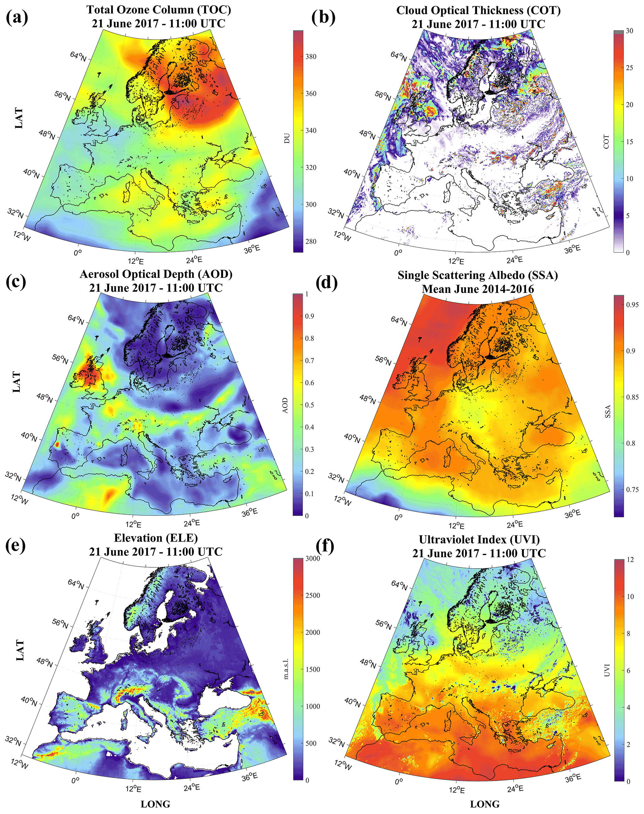
Figure 3 An example of the input TOC (a), COT (b), AOD (c), SSA (d), ELE (e) and output UVI (f) maps based on the UVIOS modeling technique applied for 21 June 2017 at 11:00 UTC.

The surface albedo data were obtained from CGLS (Geiger et al., 2008; Carrer et al., 2010). As a global surface ALB product is not available in the UV region, for this study we have used the climatological product of CGLS (in the visible range) (Lacaze et al., 2013) as follows: based on the findings of Feister and Grewe (1995), we used a UV albedo of 0.05 for non-snow cases and a UV ALB equal to CGLS when CGLS exceeded 0.5 (snow cover). The total ozone column forecasts were obtained from TEMIS, which is a near-real-time service which uses the satellite observations of total ozone column by GOME and SCIAMACHY assimilated in a transport model, driven by the ECMWF forecast meteorological fields (Eskes et al., 2003). The elevation data were obtained from the 5 min Gridded Global Relief Data (ETOPO5) database, which provides land and seafloor elevation information on a 5 min latitude–longitude grid, with a 1 m precision in the region of Europe, and is freely available from NOAA (NOAA, 1988). An analytical description of the above geophysical parameters including their specifications and resolution can be found in Table 1, followed by the corresponding references for more technical details. Figure 3 shows an example of the input–output UVIOS parameters. An extensive validation of the MACC analysis and forecasting system products was performed by Eskes et al. (2015). The aerosol optical properties were validated against 3-year (April 2011–August 2014) near-real-time level-1.5 AERONET measurements, and for AOD at 550 nm an overall overestimation was exhibited. Due to dedicated validation activity of the MACC service, a validation report that covers the time period of this study (Eskes et al., 2018) is also available, presenting an overall positive modified normalized mean bias during 2017, ranging from 0 to 0.4, with the same range of values over the study region (Europe). This overestimation of AOD at 550 nm may explain some of the UVI underestimation under clear-sky conditions (see Sect. 4.2.2).

3 Ground measurements and evaluation methodology

3.1 Ground-based measurements

In order to validate the UVIOS results, 17 ground-based stations were selected, for which measurements of the UVI were available during 2017. The stations are shown in Fig. 4. Comparisons were performed with a 15 min step. The ground-based measurements were obtained from spectrophotometers (Brewer), spectroradiometers (Bentham), filter radiometers (GUV) and broadband instruments (SL501 and YES) as Table 2 shows. Note that UV data in Table 2 have been calibrated, processed and provided directly by the responsible scientists for each station. References wherein more information for the data quality of particular instruments can be found are also provided. Brewer spectrophotometers measure the global spectral UV irradiance with a step of 0.5 nm and a resolution which is approximately 0.5 nm (usually between 0.4 and 0.6 nm). Depending on their type the spectral range is usually 290–325 nm (MKII, MKIV) or 290–363 nm (MKIII​​​​​​​). Since Brewer spectrophotometers measure the spectrum up to a wavelength which is shorter than 400 nm, extension of the spectrum up to 400 nm in order to calculate the UV index is usually achieved using empirical methods (e.g., Fioletov et al., 2003; Slaper et al., 1995). The additional uncertainty in the UVI due to the latter approximation is well below the overall uncertainty in the measurements. Bentham spectroradiometers measure the whole UV spectrum (290–400 nm) with a step and resolution which can be determined by the operator. The spectra from AOS and LIN (measured by Bentham spectroradiometers) used in this study have been recorded with a step of either 0.25 or 0.5 nm and a resolution of ∼ 0.5 nm. The Brewer spectrophotometer measures the total column of ozone using the differential absorption method, i.e., measuring the direct solar irradiance at four wavelengths and then comparing the intensity at wavelengths that are weakly and strongly absorbed by ozone (Kerr et al., 1985). Brewer TOC measurements are used in the present document to validate the TEMIS forecasts. The Ground-based Ultraviolet (GUV) instrument is a multichannel radiometer that measures UV radiation in five spectral bands having central wavelengths as 305, 313, 320, 340 and 380 nm. However, in addition to UV irradiances, other data that can be obtained from GUV instruments are total ozone and the cloud optical depth (Dahlback, 1996; Lakkala et al., 2018). GUV measurements are used for the LAN station of Norway. At stations AKR, INN and VIE, the surface UV was measured using Solar Light (SL) 501 radiometers. It provides direct observation of the UV index with a frequency of 1 min. The Yankee Environmental System (YES) has been used for the VAL station.

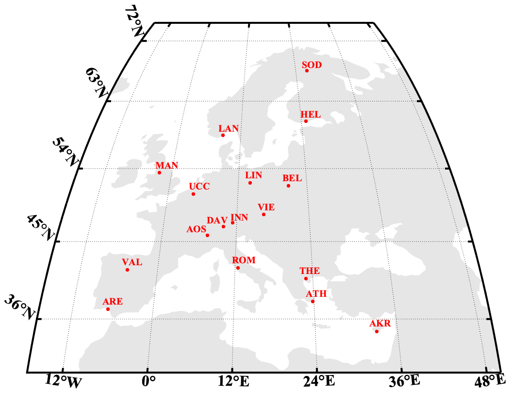
Figure 4 Study region and UVI ground measurement locations.

Table 2 Coordinates (degrees), instrument type, height (meters above sea level) and maximum UVI-measured levels of the European stations used for the comparison.

The low-latitude stations include AKR, ARE, ATH, ROM, THE, and VAL. AKR has a minimum altitude of 23 m and VAL has a maximum altitude of 705 m above sea level. The middle-latitude locations are AOS, DAV, INN, BEL, LIN, MAN, UCC, and VIE, among which the minimum altitude is 10 m in LAN and maximum altitude is in DAV at 1610 m above mean sea level. HEL, LAN, and SOD represent the high-latitude zone, with HEL having an altitude of 48 m and SOD an altitude of 185 m above mean sea level (Table 2). A summary of basic climatic information for the validation locations was obtained from the Köppen climate classification (Chen and Chen, 2013), and it is summarized here. THE, AKR, ARE, ROM, ATH and VAL have a Mediterranean climate comprising mild, wet winters and dry summers. MAN experiences a maritime climate (cool summer and cool, but not very cold, winter). AOS, UCC, LAN, BEL, HEL, LIN and VIE experience a humid continental climate with warm to hot summers, cold winters and precipitation distributed throughout the year. DAV and INN experience boreal climate characterized by long, usually very cold winters and short, cool to mild summers. SOD has a subarctic climate with very cold winters and mild summers.

3.2 Evaluation methodology

The time series period covers the whole year of 2017 at 15 min intervals, following the MSG available time steps. A synchronization between the UVIOS simulations and the ground-based measurements was performed in order to match the 15 min intervals of UVIOS to the measured data. The UVIOS data availability is 93 %, while for the ground stations it reaches almost 79 %, enabling a direct UVI data comparison of 77 % of the 2017 time steps. For the comparison we used the closest instrument measurements to the 15 min intervals with a maximum deviation of 3 min in order to avoid solar elevation and cloud presence mismatches. Additionally, the UVIOS comparisons included measurements up to 70^∘ SZA. The rationale for this cutoff was that UVIOS retrievals at high SZA are retrieved as cloudless as COT is unavailable from MSG. In addition, the comparison is also impacted by limitation of the horizon of ground-based sites (e.g., Davos, Innsbruck, Aosta) where the diffuse component and in some cases the direct component of solar UV irradiance are affected by obstacles (mountains) on the horizon. The contribution of this mainly diffuse irradiance to the total budget is a function of solar elevation and azimuth (day of the year) and also cloudiness. Although UVIOS simulations were corrected for changing UVI with respect to altitude (see Sect. 3.2.3), the correction cannot be perfect for higher-altitude stations. The reason is that it is not possible to take into account all different factors (aerosol load and properties, atmospheric pressure, surface albedo) (e.g., Blumthaler et al., 1997; Chubarova et al., 2016) which affect the change in UVI with altitude. This explains some of the deviations in the results as UVIOS retrieves UVI assuming a flat horizon. Clear-sky conditions were defined as the UVIOS retrieval where MSG COT equals zero. Further discussion on the uncertainties introduced by this choice is mentioned in the cloud effect section.

Most of the comparisons have been performed using the absolute (mean bias or median) UVI differences (model − measurements). In addition, median values of the percentage differences (100 × (model − measurements) $/$ measurements) have been used. UVIOS estimations were also evaluated in terms of mean bias and root mean square error (MBE and RMSE, respectively), defined as follows:

$$\begin{array}{}\text{(1)}& {\displaystyle }\mathrm{MBE}=\stackrel{\mathrm{‾}}{\mathit{\epsilon }}={\displaystyle \frac{\mathrm{1}}{N}}\sum _{i=\mathrm{1}}^N{\mathit{\epsilon }}_i,\text{(2)}& {\displaystyle }\mathrm{RMSE}=\sqrt{{\displaystyle \frac{\mathrm{1}}{N}}{\sum }_{i=\mathrm{1}}^N{\mathit{\epsilon }}_i^{\mathrm{2}}},\end{array}$$

where ${\mathit{\epsilon }}_i=x_{\mathrm{f}}-x_{\mathrm{o}}$ are the residuals (UVIOS errors), calculated as the difference between the simulated values (x_f) and the ground-based values (x_o), and where N is the total number of values. MBE quantifies the overall bias and detects whether UVIOS overestimates (MBE > 0) or underestimates (MBE < 0). RMSE quantifies the spread of the error distribution. Finally, the correlation coefficient (r) as well as the coefficient of determination (R²) were used to represent the proportion of the variability between modeled and measured values.

4 Results

4.1 Overall performance of the UVIOS system

Figure 5 presents a density scatterplot of the UVIOS simulations for all stations as compared to the ground-based measurements, in which a pattern of shaded squares represents the counts of the points falling in each square and which shows a correlation coefficient (r) of 0.94. For a more detailed view of the UVIOS performance, Fig. 6 depicts a Taylor diagram with the overall model accuracy for all ground stations under all-sky and clear-sky conditions as a function of the correlation coefficient, normalized standard deviation and RMSE. For both clear-sky and all-sky conditions, the results are similar. The absolute differences between UVIOS and the measured UVI are within ±0.5, and the correlation coefficients are between 0.85 and 0.99 for all the stations. The RMSE is for most stations less than 0.5. Under all-sky conditions the RMSE is higher relative to the RMSE for clear skies for MAN, DAV and SOD, which is probably due to misclassification of cloudy pixels (see also Appendix A). Relative differences can be misleading as they may correspond to very small absolute differences without physical meaning, especially for low levels of the UVI. Thus, we focused on absolute differences in order to have a more representative assessment of the actual effect (UV index) and its results. The differences were categorized as low (less than 0.5), moderate (0.5–1) and high (more than 1). In Appendix A, relative differences are also discussed.

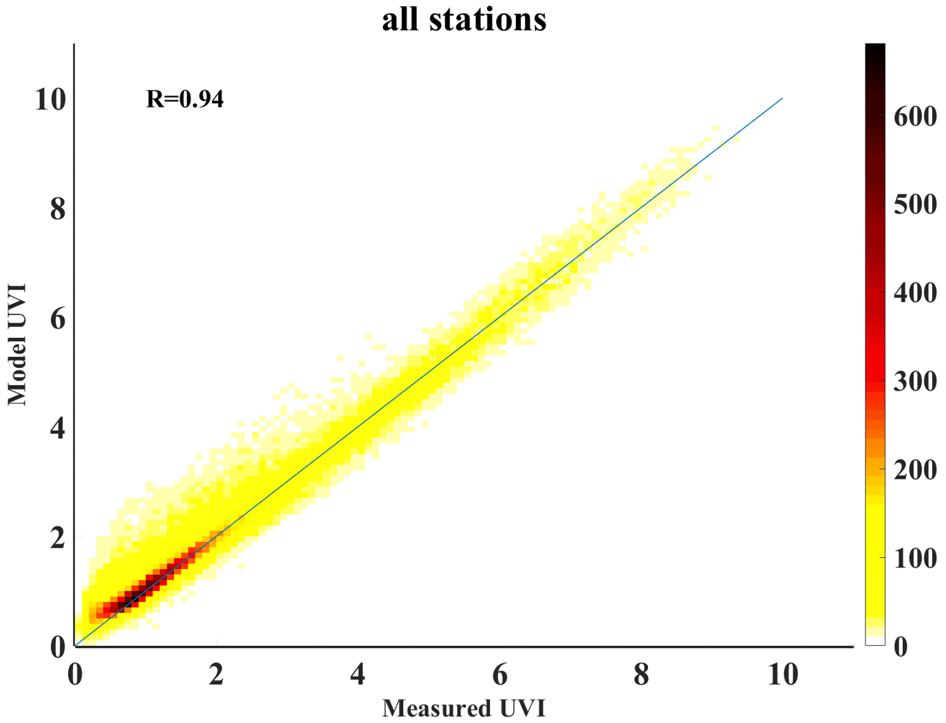
Figure 5 Density scatterplot of the overall UVIOS performance for all stations. The analytical statistics for each station can be found in Appendix A.

Figure 6 Taylor diagram for the overall UVIOS accuracy for all ground stations under all-sky (a) and clear-sky (b) conditions.

In Table 3, U1.0 and U0.5 represent the percentage of cases with absolute differences between modeled and ground-based UVI measurements within 1 and 0.5, respectively, for all comparisons between the 15 min model retrievals and the corresponding ground-based measurements. As shown in Table 3, for all stations and for both clear- and all-sky conditions, differences were within 0.5 UVI for at least 70 % of the cases. Under clear-sky conditions, AOS, BEL, HEL, LAN, LIN, SOD and THE had above 90 % of U0.5 cases, while others had 75 %–90 % of U0.5 cases. All stations but DAV had above 90 % of U1.0 cases for clear skies, while the correlation coefficients for most of the stations were above 0.9 (exceptions are ATH and MAN). For all skies differences were within 1 UVI for 90 % of the cases for all stations, with the correlation coefficients exceeding 0.9 for most of them (exceptions are DAV, MAN and SOD). Median differences for all skies for every station were well within ±0.2 UVI, with the 25th–75th percentiles being within ±0.5 UVI and the 5th–95th percentiles within ±1 UVI. For clear skies the corresponding values are ±0.1, ±0.4 and ±0.8, respectively. In the following sections we try to investigate the factors that contribute to the differences between UVIOS and ground-based measurements.

Table 3 Absolute difference between UVIOS and ground-based UVI measurements in terms of percentages (%) of data that are within 0.5 and 1 UVI of difference (U0.5 and U1.0, respectively) as well as the correlation coefficient (r) for all-sky and clear-sky conditions.

4.2 Factors affecting UVIOS retrievals

4.2.1 Ozone effect

All the available collocated TOC measurements for the stations used in the UVIOS evaluation have been obtained from the WOUDC (https://woudc.org/, last access: 22 October 2020) database. In this database 8 out of 17 UVIOS evaluation stations (AOS, ATH, DAV, MAN, ROM, SOD, THE and UCC) were found, providing TOC ground-based measurements. TOC comparison has been performed by calculating daily means of ground-based measurements and the TOC from TEMIS. In order to quantify the effect of the uncertainty of the forecasted TOC used as input at UVIOS, we have calculated the mean differences of the forecasted and measured TOCs and used a radiative transfer model to investigate their effect on the UVIOS-retrieved UVI. Table 4 shows the mean differences in DU from TEMIS TOC (used as inputs in UVIOS) as compared to the WOUDC ground-based measurements for 1 year of comparison data. It is seen that for the stations AOS, DAV, MAN and UCC the values of the TEMIS observations are higher as compared to the ground-based measurements (by 7.6, 1.9, 5, and 2.9 DU, respectively), while for the other stations TEMIS observations are lower (by 0.9, 5.4, 9.9, and 2.2 DU for ATH, ROM, SOD, and THE, respectively). The negative bias is seen to be highest for the ROM station (−9.9), and the positive bias is highest for the AOS station (7.6). Part of the large differences over the complex terrain sites can be explained by the difference between the actual altitude of the station and the average altitude of the corresponding grid points of TEMIS. For example, for AOS the average altitude of the pixel is 2000 m, while the real altitude of the station is 570 m, resulting in an underestimation of the tropospheric column of ozone by TEMIS. In general, differences can be explained by the combined effects of uncertainties in TOC retrieval from satellite and ground-based platforms (Rimmer et al., 2018; Boynard et al., 2018; Garane et al., 2018). Figure 7 shows the effect of this TOC bias on the calculated UVIOS. As seen in Table 4, there is a mix of small underestimation and overestimation cases in the TOCs used within UVIOS, with average absolute differences of 4–5 DU. The worst TOC UVIOS inputs were found in AOS and ROM (7.6 and −9.9 DU), leading to maximum (at 30^∘ SZA) differences in UVI of −0.22 and 0.3 for AOS and ROM, respectively. In general, in most of the cases UVI mean differences are less than 0.1. It has to be noted that the TOC differences have a larger impact when expressed in percent at higher SZAs, while in Fig. 7 higher absolute differences for low SZAs are associated with higher UVIs at these SZAs. Detailed comparisons for each station are shown in the Appendix A figures.

Table 4 Mean bias error of the TEMIS TOC as compared to the WOUDC ground-based measurements.

Figure 7 Differences of UVI derived by UVIOS using as input the TEMIS and Brewer TOC, respectively, at all stations with available data (lower possible SOD SZA is 44^∘).

4.2.2 Aerosol effect

Aerosol optical depth measurements used for the UVIOS aerosol input evaluation have been collected from the AERONET-NASA web site (Giles et al., 2019) for 12 out of our total of 17 stations (AKR, ARE, ATH, DAV, HEL, LIN, ROM, SOD, THE, UCC, VAL and VIE). AERONET (level 2, version 3) values of AOD at 500 nm were interpolated at 550 nm using the AERONET-derived 440–870 nm Ångström exponent for each individual measurement. In order to compare those measurements with CAMS-forecasted AOD used for UVIOS, their daily means were derived. The comparison of forecasted and measured daily means was based on all available data due to gaps in the AERONET time series. The AOD MBE and RMSE statistical scores are shown in Table 5 in absolute units and correlation coefficient as well. All the stations have a mean positive bias up to 0.071 except UCC, which shows a mean negative bias of 0.007. The comparison of all individual stations with CAMS data used as inputs on UVIOS showed that under all cases CAMS AOD is higher than that from AERONET with a mean difference of 0.07 at 550 nm. The correlation between the modeled and measured values varies from 0.10 for VIE to 0.91 for ARE, with most of the stations showing the correlation coefficient above 0.7. As in the case of the TOC, AOD CAMS data are forecasts from the previous day and real-time WOUDC or AERONET level 2.0 data do not exist. Although real-time TOC (and in due course AOD in the UV) is available from Eubrewnet (López-Solano et al., 2018; Rimmer et al., 2018), it is only for particular locations and not for the whole European domain. Thus, the only choice in providing for a real-time UV index for Europe is using the CAMS (for AOD) and TEMIS (for TOC) data.

Table 5 Comparison results between CAMS-forecasted AOD values used as UVIOS input and AERONET ground-based AOD measurements. The AOD MBE and RMSE statistical scores are shown in absolute units along with the correlation coefficient.

In order to evaluate the effect of AOD on UVI, UVI differences between the UVIOS using both AOD data sets (CAMS and AERONET) as UVIOS inputs were analyzed. Figure 8 shows the mean bias error of the CAMS–AERONET AOD impact on UVI for all stations with available ground-based AOD data as a function of SZA together with the uncertainty range (±1σ). It can be seen that UVIOS with CAMS AOD input underestimates UVI compared to UVIOS with AERONET data, except for the UCC station. This is consistent with CAMS overestimations of AOD compared to the AERONET measurements, except for the UCC station as shown in Table 5. Higher aerosol levels in the atmosphere tend to lower the UVI. The highest difference in UVI is observed for the stations HEL, SOD, and VIE. Since the aerosol level at the stations HEL and SOD is very low, the percent difference between the AOD from CAMS and AERONET is larger for these stations (although the absolute difference is similar) relative to stations with higher AOD, leading to higher differences in the UVI. Aerosol content for VIE is higher than HEL and SOD but still within 0.2, which might be the reason for the higher UVI difference. In terms of SZA, it is observed that the mean bias decreases with an increase in the SZA as the values of UVI also decrease with SZA, and the most deviation is for station VIE, which is consistent with the poor correlation between the CAMS-forecasted input and the measurements for this station as seen from Table 5.

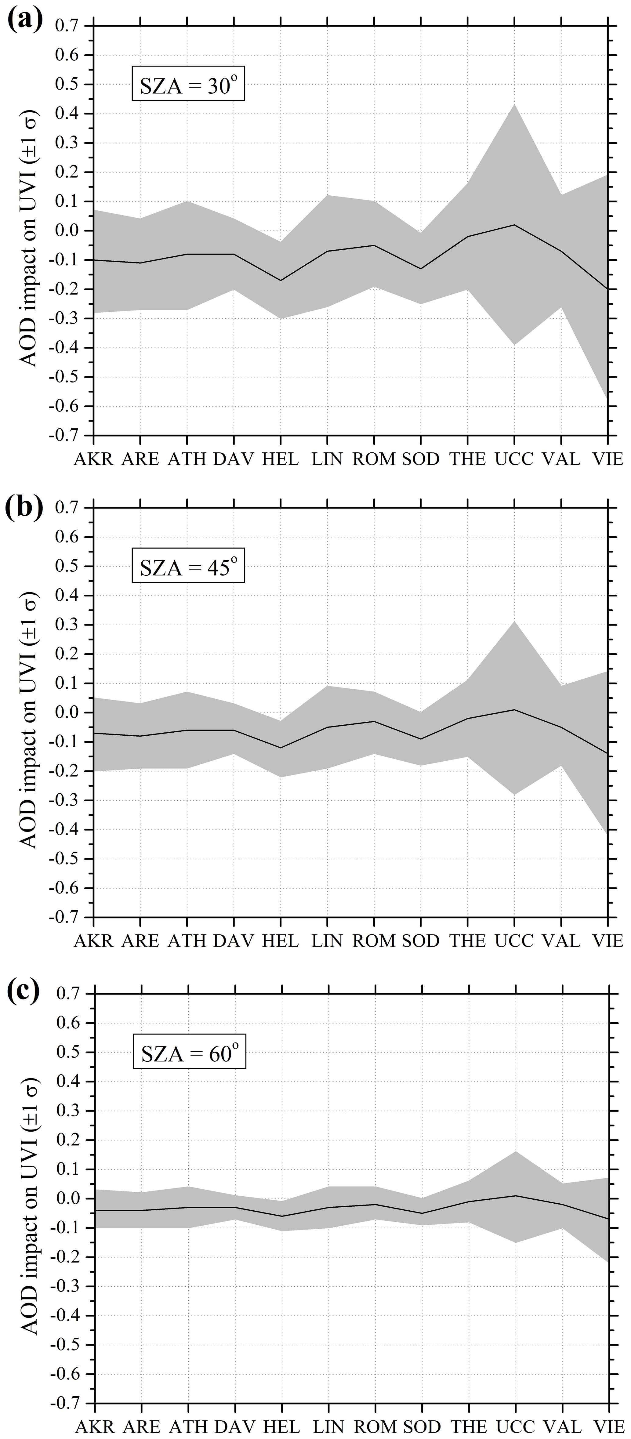
Figure 8 The mean bias error of the CAMS–AERONET AOD impact on UVI for all stations with available data as a function of SZA at 30^∘ (a), 45^∘ (b) and 60^∘ (c) together with the uncertainty range (±1σ).

The use of single scattering albedo in the UV region is a difficult task, and many studies have shown that such measurements need extra effort, and it is not possible to perform them worldwide (Arola et al., 2009; Kazadzis et al., 2016; Raptis et al., 2018). The monthly values of the single scattering albedo used in UVIOS for the UV region were derived from the MACv2 database at the 310 nm wavelength (Kinne, 2019). Figure 9 shows the intra-annual variability of SSA for the 17 stations. For all stations, SSA values range from 0.76 to 0.93, with most of them having SSA values between 0.83 and 0.93 and relatively small variability. In contrast, there are stations like ARE, BEL, INN, LIN, VIE and THE which have relatively smaller SSA values (0.76–0.9) and greater variability than the other stations.

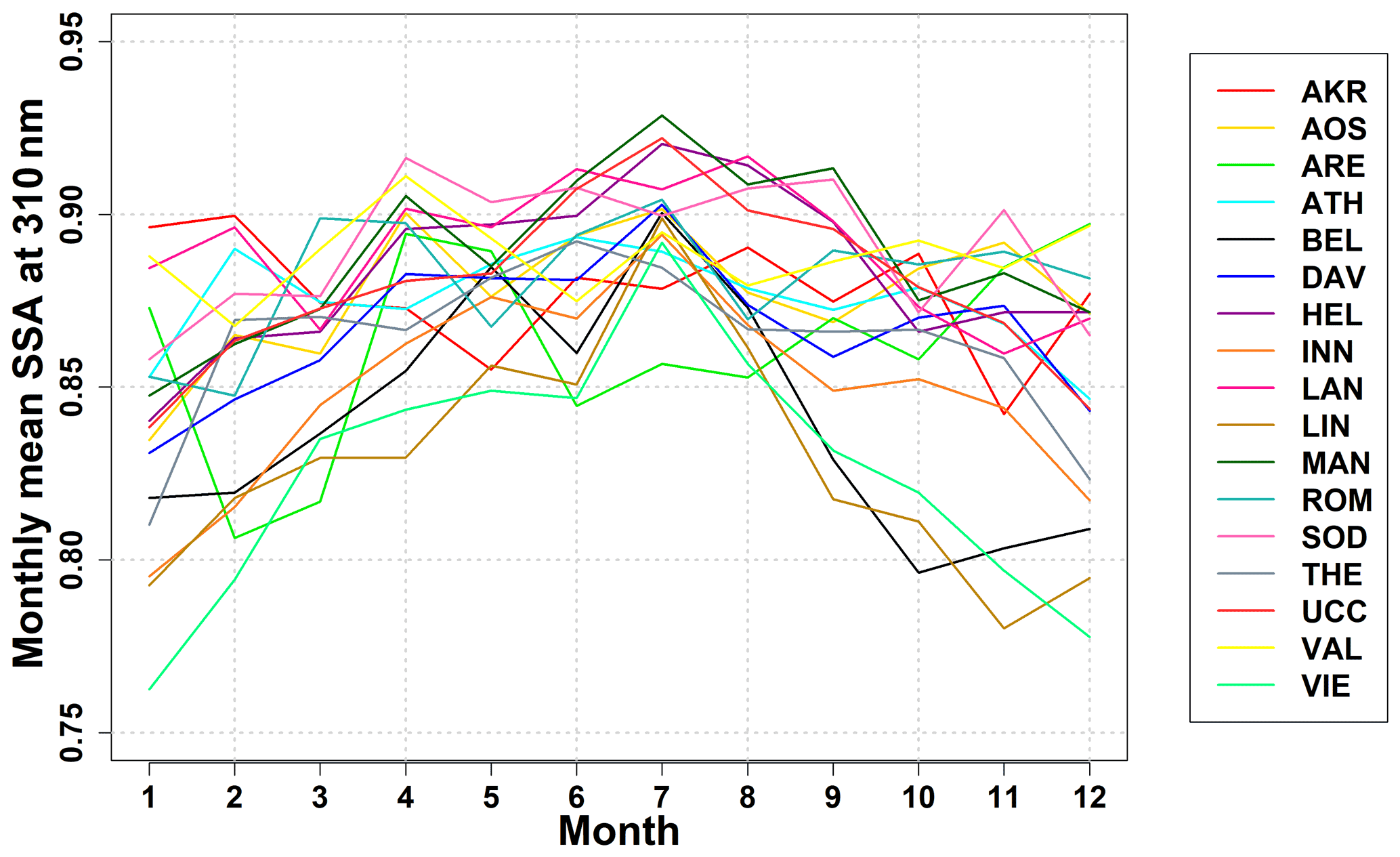
Figure 9 The monthly mean (i.e., 1–12 = January–December) SSA levels for all ground stations as derived by the MACv2 database.

4.2.3 Albedo effect and surface elevation correction

Surface albedo at UV wavelengths is small (2 %–5 %) for most types of surfaces (Feister and Grewe, 1995; Madronich, 1993) except for features like sand (with a typical albedo of ∼ 0.3) and snow (up to 1 for fresh snow) (Meinander et al., 2013; Myhre and Myhre, 2003; Vanicek et al., 2000; Henderson-Sellers and Wilson, 1983). Renaud et al. (2000) found an enhancement of about 15 % to 25 % in UVI for clear skies and snow conditions due to the multiple ground–atmosphere reflections, and this relative increment was about 80 % larger for overcast conditions. The combined effect of aerosols and snow led to an enhancement of about 50 % in UVI in cloud-free conditions for moderately polluted atmospheres (Badosa and Van Weele, 2002). Figure 10a presents the effect of surface albedo on the UVI percentage difference (i.e., for various albedo values under clear-sky conditions) as a function of SZA, while Fig. 10b shows the effect of surface elevation on UVI as a function of the percentage difference for various total ozone columns. It is observed that the UVI percentage difference increases almost linearly with albedo for a particular SZA, and the variation is found to be almost identical for all SZAs. This indicates that the UVI percentage difference is independent of the SZA and increases with surface albedo. The UVI percentage difference is found also to increase almost linearly with the increase in elevation for a particular total ozone column. The percentage difference is similar for all ozone columns up to 1 km, after which the differences with ozone column become more apparent. That is, at a particular elevation, the percentage difference is higher for less total ozone column. A 1 % fluctuation (decline or increase) in column ozone can lead to about a 1.2 % fluctuation (increase or decline) in the UV index (Fioletov et al., 2003; Probst et al., 2012). Indicatively, the average maximum surface elevation correction in terms of UVI for the DAV station (due to UVIOS input deviation from the actual elevation) was on the order of 1.6 (15 %), while for INN and AOS it was 0.5 and 0.6, respectively (6 %), and for the VAL station close to 0.8 (8 %).

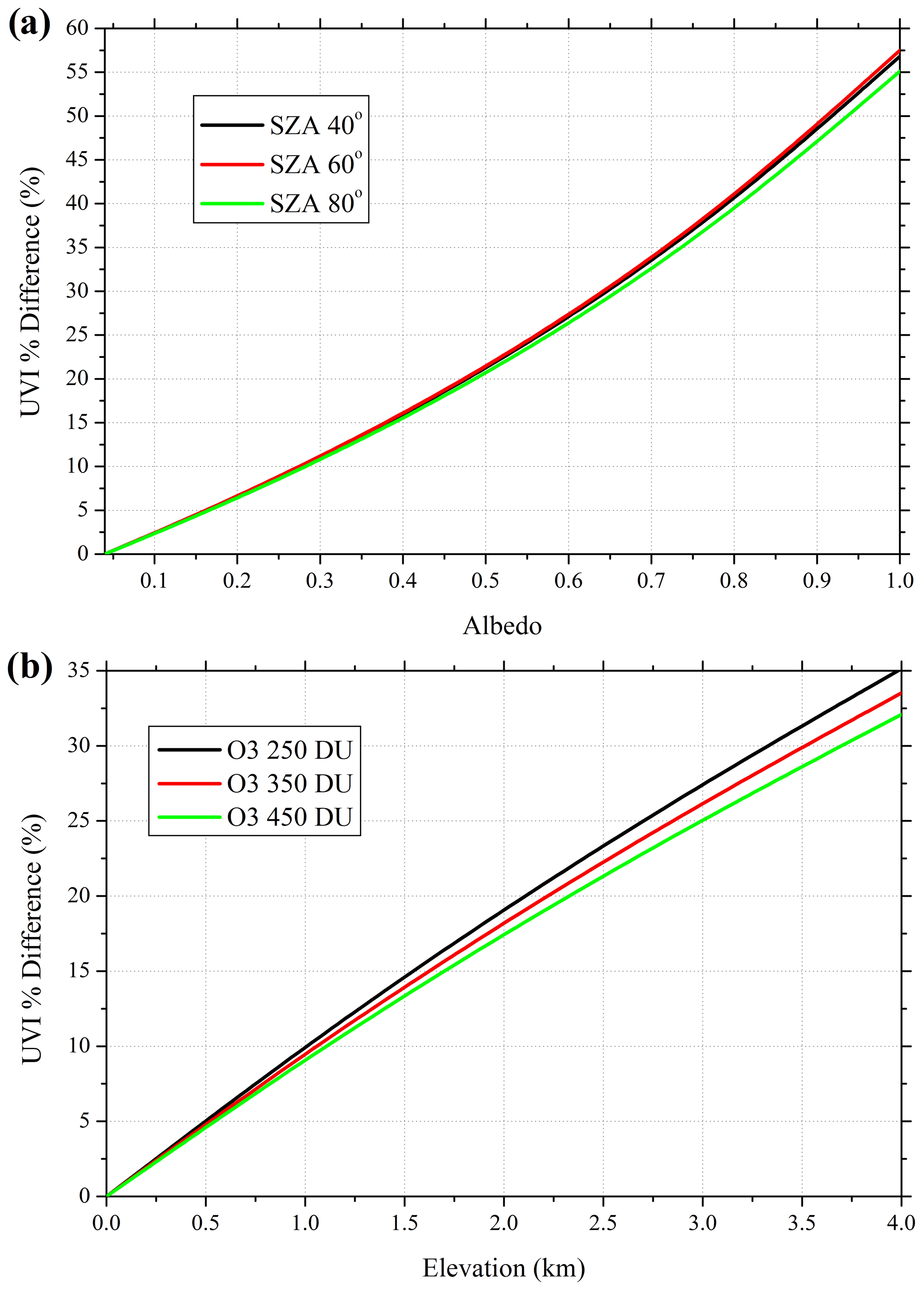
Figure 10 The surface albedo effect on UVI as a function of percentage difference for various SZAs (a). The surface elevation effect on UVI as a function of percentage difference for various total ozone columns (b).

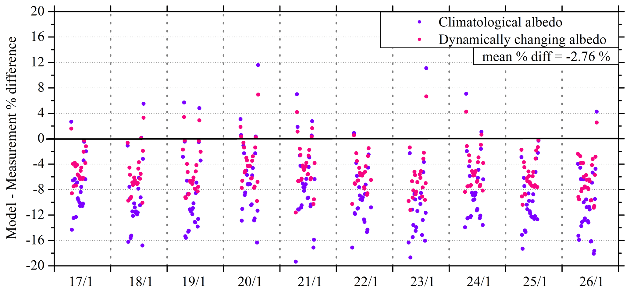
Figure 11 The effect of surface albedo correction on UVI for the Davos station. The climatological and dynamically changing albedo in terms of percentage differences of modeled and ground measurements during a snow-covered period (17–26 January) under clear-sky conditions.

Uncertainties introduced in UVIOS from the use of a constant surface albedo value of 0.05 for non-snow conditions are quite low. For the case of albedo values used for snow conditions based on the CGLS monthly mean product, uncertainties can be related to the small difference of UV and visible albedo values; the fact that the CGLS provides an albedo of a certain area around the station that does not necessarily coincide with the “effective” albedo area affecting UV measurements; and finally that the monthly albedo product represents a monthly average, while a real-time CGLS product represents the last 12 d (dynamically changing albedo). In order to investigate this last point, we have compared the UV effects from the use of the two albedo data sets for the DAV station, where the average difference between an example ground-based data set and UVIOS was found to be 0.14 UVI (Gröbner, 2021). In Fig. 11, the effect of surface albedo correction is shown for the Davos station for a period with snow cover and low-percentage cloudiness. The climatological and dynamically changing albedos are presented in terms of percentage differences between modeled and ground measurements as a function of SZA. In the case of climatological albedo, most of the percentage difference between the forecasted and measured UVI values is found to vary from −30 % to 10 % for SZA between 20 and 70^∘, showing more underestimation than overestimation from the UVIOS simulations. Similarly, in the case of dynamically changing albedo, most of the percentage difference between the forecasted and measured UVI values is found to vary from −20 % to 10 % for SZA between 20 and 70^∘. The mean percentage difference between the results using the two different albedo inputs is −2.76 % in terms of accuracy improvement. However, beyond 70^∘ SZA, there is a huge variation in the percentage difference, with mostly underestimations from the UVIOS simulations (not shown in Fig. 11).

4.2.4 Cloud effect

For the evaluation we used measurements at SZA lower than 70^∘, based on the lack of cloud input from MSG for higher SZAs. The lack of MSG data results in an overestimation of UVIOS in high SZAs, and the UVI is systematically overestimated for long periods during winter in high-latitude regions when SZA does not get below 70^∘ during the day. However, based on the simulations performed by UVIOS, this overestimation is low in terms of absolute UVI and does not usually exceed 0.2 UVI because maximum UVIs at such SZAs rarely exceed UVI = 1.

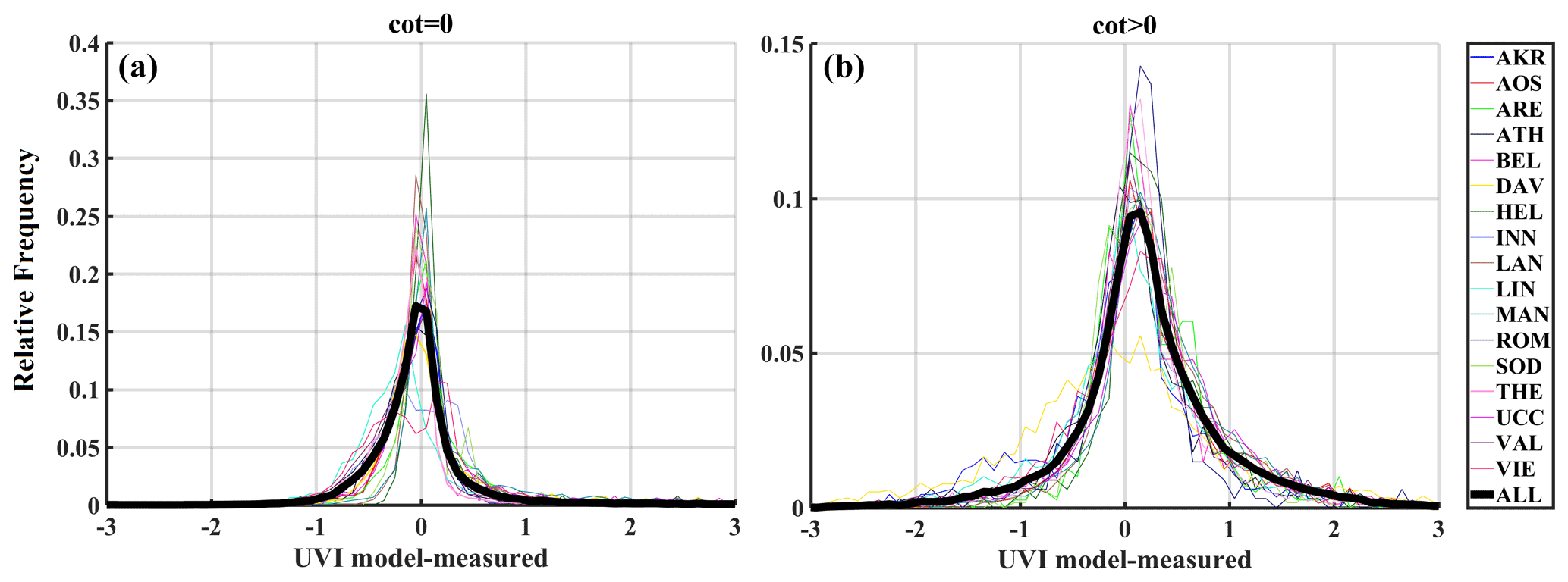
Figure 12 Relative frequency distribution of UVI residuals for all stations (colored lines) and the mean (bold black line) for cloudless (a) and cloudy (b) conditions.

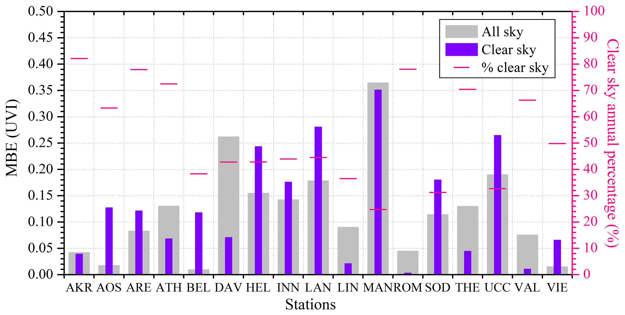
Figure 13 Mean bias error of the modeled UVI as compared to the ground-based measurements for all-sky and clear-sky conditions. The percentage of clear-sky data time steps was also plotted with red lines.

COT retrieved from the MSG satellite has been used as input for UVIOS together with typical optical properties of the clouds as discussed in Sect. 2.1. The evaluation of all stations for cloudless and cloudy conditions can be seen in Fig. 12, which shows the relative frequency distribution of all stations (colors) and the mean (black line) for cloudless (upper plot) and cloudy conditions (lower plot). Mean bias error of that modeled by UVIOS and measured UVI for all-sky and clear-sky conditions and the percentage of clear-sky time-step data is presented in Fig. 13. The mean bias for clear-sky conditions is found to be less than that for the all-sky conditions for the stations AKR, ATH and THE (having most days of the year being cloudless as the clear-sky percentage is above 70 %). The MBE for DAV, LIN and MAN is less for clear sky relative to all-sky conditions even though most days of the year are cloudy (clear-sky annual percentage less than 45 %) at the particular stations, while stations BEL, HEL, INN, LAN, SOD, UCC and VIE, which have mostly cloudy skies throughout the year (clear-sky annual percentage less than 50 %), have more MBE for clear-sky conditions than the all-sky condition. This can be due to the erroneous classification of a cloudy sky as clear sky, which is also discussed in the following section. MBE is also larger for AOS and ARE, which have mostly clear skies throughout the year. Stations ROM and VAL have comparatively much smaller MBE for clear-sky conditions.

Table 6 Percentage of data for UVIOS underestimation (A1–A3) and overestimation (B1–B3) under clear- and cloudy-sky conditions for various UVI difference (modeled-ground) classes.

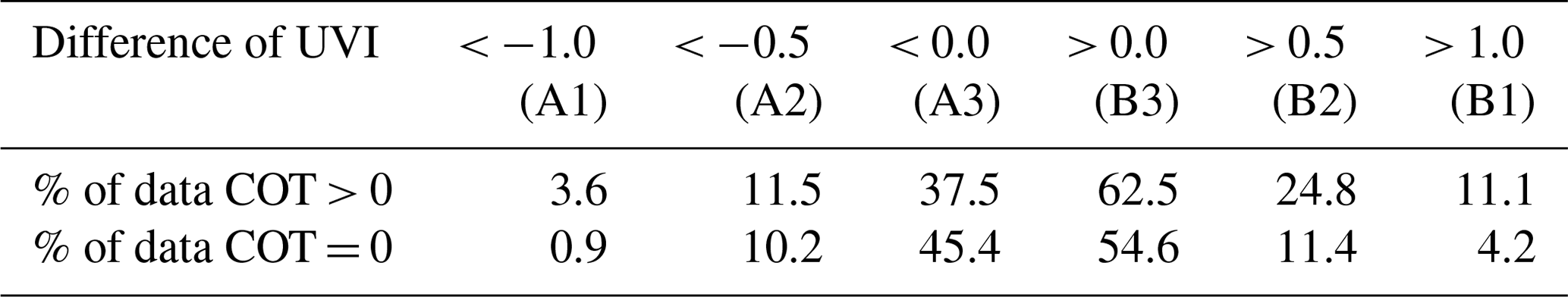
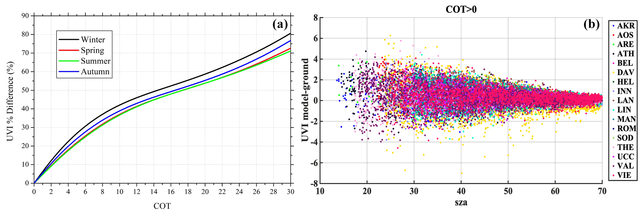
Figure 14 The average COT effect on UVI as a function of percentage difference for all seasons (a) and scatterplot of the UVI difference under cloudy-sky conditions for all stations (b).

As shown in Table 6, there are 45.4 % of cases with underestimations and 54.6 % of cases with overestimations for cloudless conditions (COT = 0). For all the other cases, overestimations (62.5 %) are more predominant than underestimations (37.5 %). The difference in the modeled and measured values goes beyond ±1 UVI for only 5.1 % of cases for cloudless conditions and 14.7 % for all the other cases. In general, under cloudy conditions, UVIOS shows an overestimation for UVI, in contrast to the ground measurements. One explanation for these estimates' inaccuracy could be the erroneous determination of COT from MSG above the ground-based stations, giving cloud input to UVIOS that can be overestimated or underestimated. The results show that there is a general tendency for a small underestimation of MSG COT that leads to a systematic but small UVIOS UVI overestimation under cloudy conditions. Another possible explanation is the spatial representativeness of MSG COT. The MSG COT determination is available at 5 by 5 km pixels that may differ from the actual situation of the cloud prevailing above the station, especially in broken cloud conditions and in cases when it blocks the direct radiation from the Sun. Moreover, for lower solar elevations, the direct Sun irradiance can be blocked by cloud in neighboring pixels. The first effect has been explored in the relative frequency distribution of Fig. 12 that shows a higher number (∼ 63 %) of data on the right of the zero UVI difference vertical line for cloudy skies. When comparing data outside the 0.5 and 1 difference limits, we also see that 1–4 times more data show a UVIOS overestimation as compared to the clear-sky case. This shows that in general there is a small (in UVI terms) but significant UVIOS overestimation for non-zero COT conditions. Moreover, for clear skies, as determined from the MSG, we observe a less pronounced UVIOS overestimation that corresponds to the fact that even if MSG defines the situation as completely cloudless, in reality there may be some cases where clouds near the ground-based station affect the measured UVI. This effect is easier to understand when showing these differences as a function of solar zenith angle which is explored through Fig. 14. It is observed that the absolute difference between the modeled and measured values decreases with increasing solar zenith angle, and most of the difference lies within ±4 UVI. The seasonal variation of the percentage UVI difference as a function of SZA shows that while absolute UVI is small in winter, the percentage difference is higher compared to other seasons.

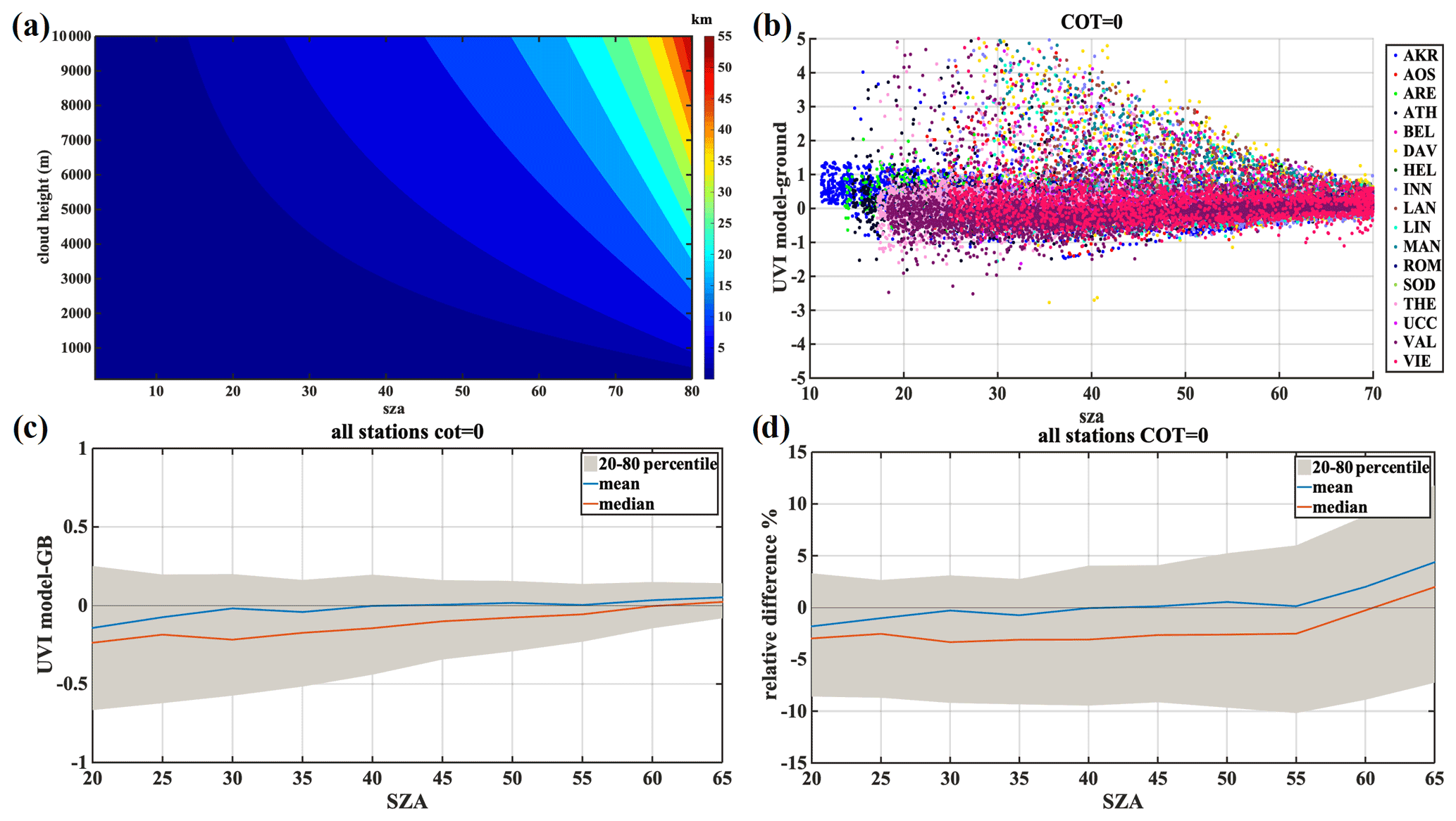
Figure 15 The shadow volume at the surface level of a cloud relative to the SEVIRI angle view as a function of cloud height and SZA (a). Scatterplot of the UVI difference under clear-sky conditions for all stations (b). UVI mean, median and 20th–80th percentile differences (c) and percentage differences (d) derived by UVIOS as compared to the ground-based measurements for clear-sky conditions as a function of SZA.

Figure 15a shows the shadow volume at the surface level of a cloud, relative to the SEVIRI angle view, as a function of cloud height and SZA, highlighting the ray tracing in the presence of clouds and the accompanying angular dependence due to the 3D geometry. Figure 15b shows the scatter of the UVI difference under clear-sky conditions for all stations as a function of SZA. It is observed that there is an obvious pattern of scattered data for UVI differences higher than 1.5 compared with the ones for differences less than −1.5. These data represent UVIOS overestimation for UVI retrievals due to the underestimation of the cloudiness just above the stations. These data illustrate the well-known spatial representativeness issues whereby a COT value for a satellite grid is not fully representative of a point measurement station. In addition, absolute and percentage relative differences are shown in Fig. 15c and d, respectively, for SZA up to 65^∘. The differences between UVIOS and the ground-based UVI decrease in absolute level but increase in percent, with an increase in SZA. This is due to the decrease in UVI with increasing SZA. Modeled and measured UVI difference is close to zero for both mean and median values. For SZA below 30^∘, differences are 0 to −0.2, while the 20th to 80th percentiles range from −0.6 to −0.2. Percentage difference increases with SZA as absolute UVI decreases, with the 20th to 80th percentiles showing differences between −10 % and 10 %.

5 Conclusions and future plans

In this study, a fast RTM model of UVI, the so-called UVIOS, using inputs of the SZA, aerosol optical depth, total ozone column, cloud optical depth, elevation and surface albedo that implicitly includes temporal effects and the effect of cloud and aerosol physics allows for the generation of high-resolution maps of UVI. Ground-based measurements of UV are the most accurate way to determine this important health-related parameter. However, such stations are sparse, and hence satellite observations can be used in order to have a nowcasted UV service. To date, polar-orbiting satellites like TOMS, OMI and recently TROPOMI have provided a global UV data set, with a major disadvantage being the temporal resolution (one measurement per day). This combined with the large temporal variability of clouds can lead to huge deviations from reality when a single daily measurement is included. Geostationary satellites, MSG, have been used in order to try to improve on such limitations using cloud information every 15 min.

Comparison of the forecasted and ground-based measurements indicated that at least 70 % and 80 % of comparisons were within 0.5 UVI difference for all-sky and clear-sky conditions, respectively. The mean differences between TEMIS TOC and the ground-measured TOC from the WOUDC for 1 year of comparison data showed that TEMIS tends to slightly overestimate the TOC for some stations along with underestimating it for other stations. While, in general, in most of the cases UVI mean differences are less than 0.1, the TOC differences have a larger impact in percent UVI differences at higher SZAs. Such small differences can also be the result of daily TOC variation not captured in TEMIS.

CAMS AOD seems to be slightly overestimated as compared with AERONET data, which leads to a UVIOS underestimation. CAMS data are found to overestimate the AOD from AERONET measurements, with a mean difference of 0.07 at 500 nm. All the stations have a mean positive bias up to 0.071 except one station, which had a mean negative bias of 0.007. The analysis of the impact of the mean bias error of the CAMS–AERONET AOD impact on UVI for all stations showed that the mean bias decreases with an increase in the SZA as the values of UVI also decrease with SZA. The greatest deviation is for station VIE, which is consistent with the poor correlation between the CAMS-forecasted input and the measurements for this station. The real-time data provision approach of UVIOS requires using a maximum of 1 d ozone and aerosol forecast using the TEMIS and CAMS service, respectively. Uncertainties in the used SSA increase the overall uncertainty of the simulated UVI, especially for high levels of atmospheric aerosols. However, as systematic SSA measurements in the UV region are not available, quantification of these uncertainties was not possible.

Cloudy conditions show high percentage differences but low UVI differences and have a general tendency to lead to a UVIOS overestimation. It was found that 45.4 % of cases have underestimations, while 54.6 % of cases have overestimations for the cloudless conditions, and overestimations (62.5 %) were more predominant than underestimations (37.5 %) for all the other cases. In general, UVIOS showed an overestimation for UVI, in contrast to the ground measurements under cloudy conditions, with the difference in the modeled and measured values going beyond ±1 for 5.1 % of cases for cloudless conditions and 14.7 % for all the other cases. At individual stations, the results for cloudless sky conditions, which are the most important for health-related issues, showed good agreement. In general, ∼ 85 % of all cases and 95 % of cloudless cases are within 1 UVI difference. The relative percentage biases can be large for low UVI cases due to clouds or at high SZAs, above 75^∘, due to the absence of accurate information for clouds. The results show that there is a general tendency of small underestimation of MSG COT that leads to a systematic but small UVIOS overestimation under cloudy conditions. Another possible explanation is the spatial representativeness issues between a satellite and a single point on the ground.

Using climatological surface albedo has little impact at low-albedo sites but mainly leads to underestimations in UVIOS simulations for high-albedo situations (snow cover). Most of the percentage difference between forecasted and measured UVI values varied from −30 % to 10 % for SZA between 20 and 70^∘ (climate albedo), while it was found to vary from −20 % to 10 % for dynamically changing albedo. Since high surface albedo conditions correspond to winter months (i.e., high SZAs and relatively low UVI) for the stations used in the study, the corresponding absolute differences in the UVI are generally smaller than 2 UVI. However, there was a huge variation in the percentage difference beyond 70^∘ SZA, with mostly underestimations from the UVIOS simulations. Finally, for uncertainties in elevation inputs, the UVI percentage difference is found to increase almost linearly with the increase in elevation for a particular total ozone column, and beyond that, it is seen that the rate of increase in the percentage difference decreases with increase in the total ozone column.

The UVIOS system forms a novel tool for widespread estimations of UVI using real-time and forecasted EO inputs. UVIOS utilizes the MSG domain with high spatiotemporal resolution, producing outputs within acceptable limits of accuracy for UV health-related applications. It captures basic cloud features and all major atmospheric and geospatial parameters that affect UVI. Under cloudless conditions it performs to within the uncertainty of the ground-based measurements to which it has been compared. Further development and improvement of the model can be achieved in the future. Meteosat Third Generation (MTG) satellites are expected to be launched in the following years and give aerosol and cloud products which would improve the performance of nowcast and forecast UV models when used as inputs. A future goal is to compare the UVIOS accuracy under cloudy conditions by using (i) the current MSG cloud information (5 km, 15 min), (ii) the ECMWF forecast cloud information (4 km, 1 h) and (iii) the forthcoming MTG cloud information (500 m, 5 min) in order to quantify the uncertainties of the forecasted cloud data as compared to the satellite observations as well as the overall improvement of the MTG data compared to the MSG due to the MTG's higher resolution.

The future plans with the UVIOS system include open access to the operational UVI product through European online map-based user interfaces, data hubs and cloud platforms for Earth observation data (e.g., GEOSS Portal and NextGEOSS). A real-time correction and quality assurance of the outputs are also scheduled by assimilating ground measurements in collaboration with the stations used in this study. In addition, the short-term and long-term forecasting horizons will be exploited for further added value as an early warning system that raises awareness among citizens of the health implications of high UVI doses. In this direction, numerical weather prediction models and computer vision techniques (Kosmopoulos et al., 2020) will be utilized as complements to the UVIOS system in order to capture the cloud movement forecast and effect on the UVI levels. Finally, a historical database of UVI will be developed by using climatological input data sources for past years aiming to study climatic trends and to make the system a holistic platform for scientific and social value deployment.

Appendix A

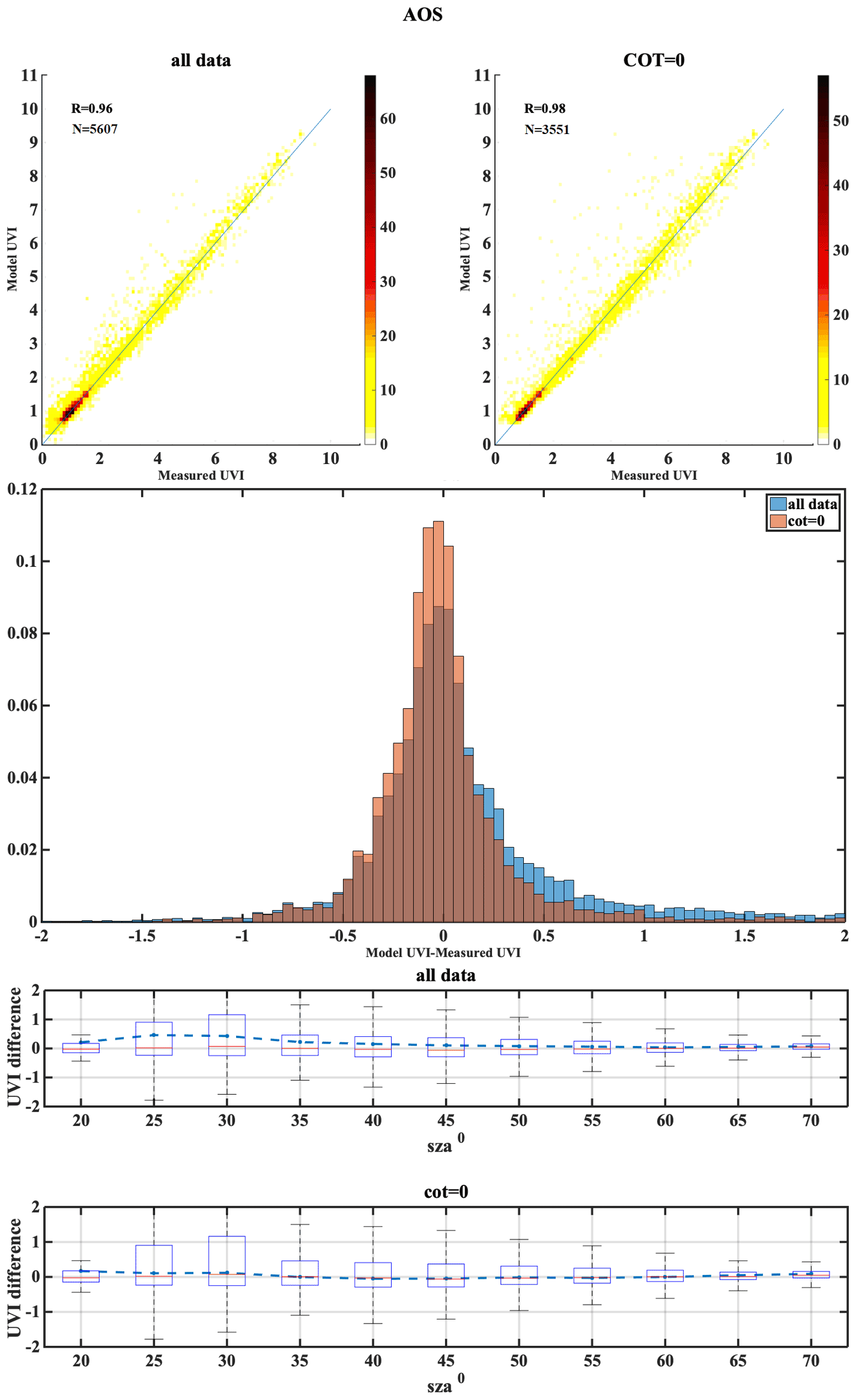
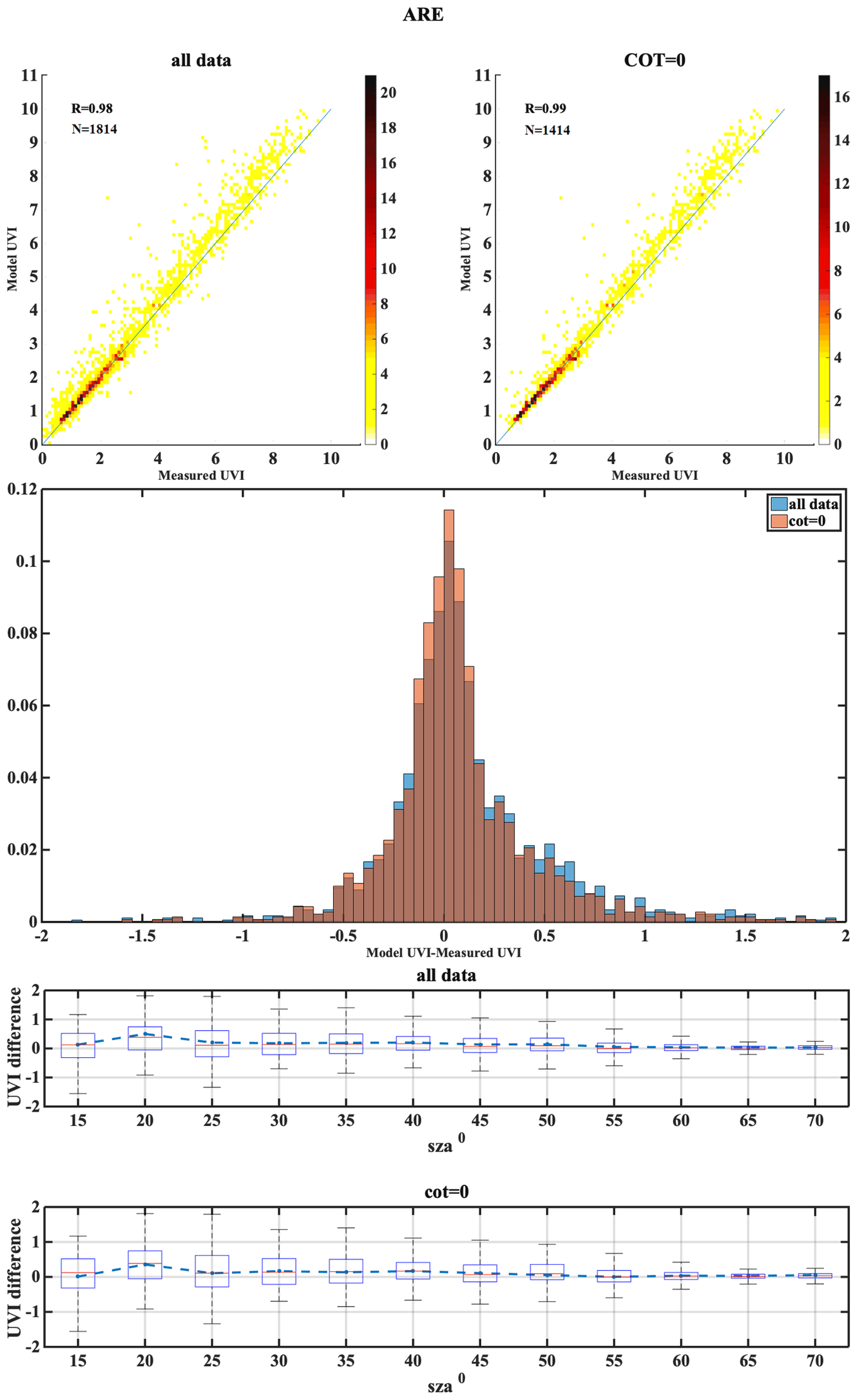
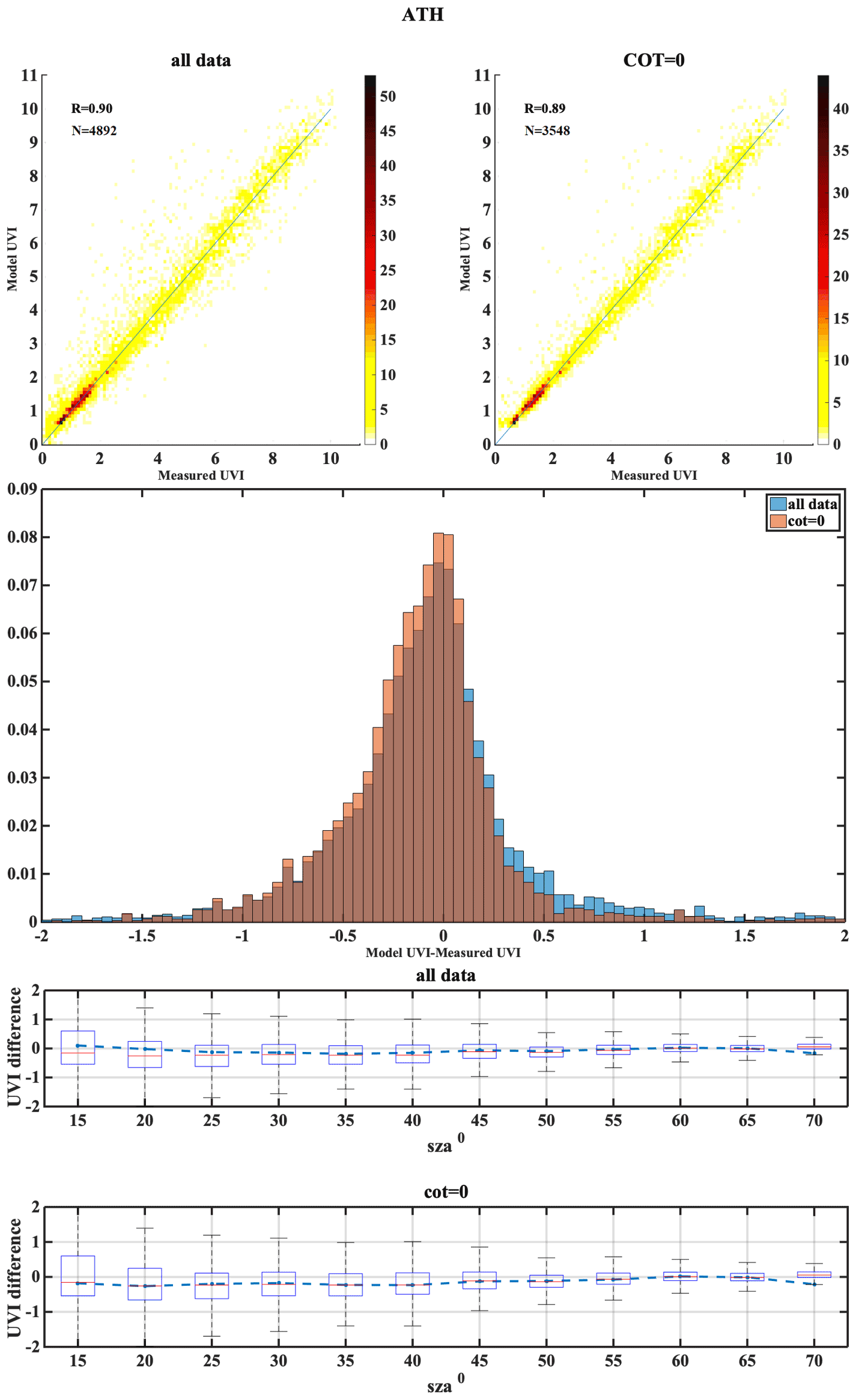
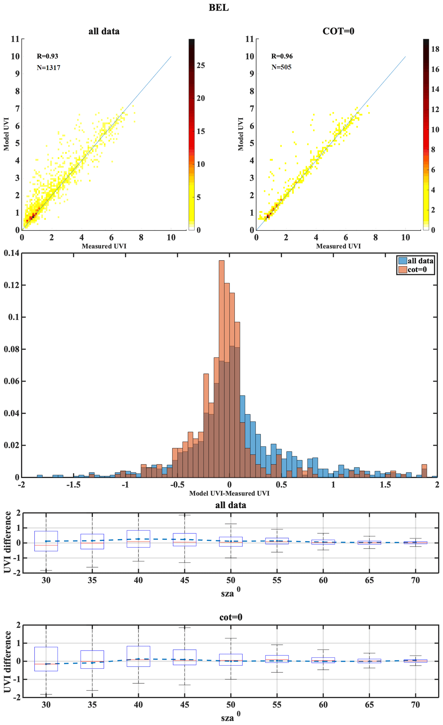
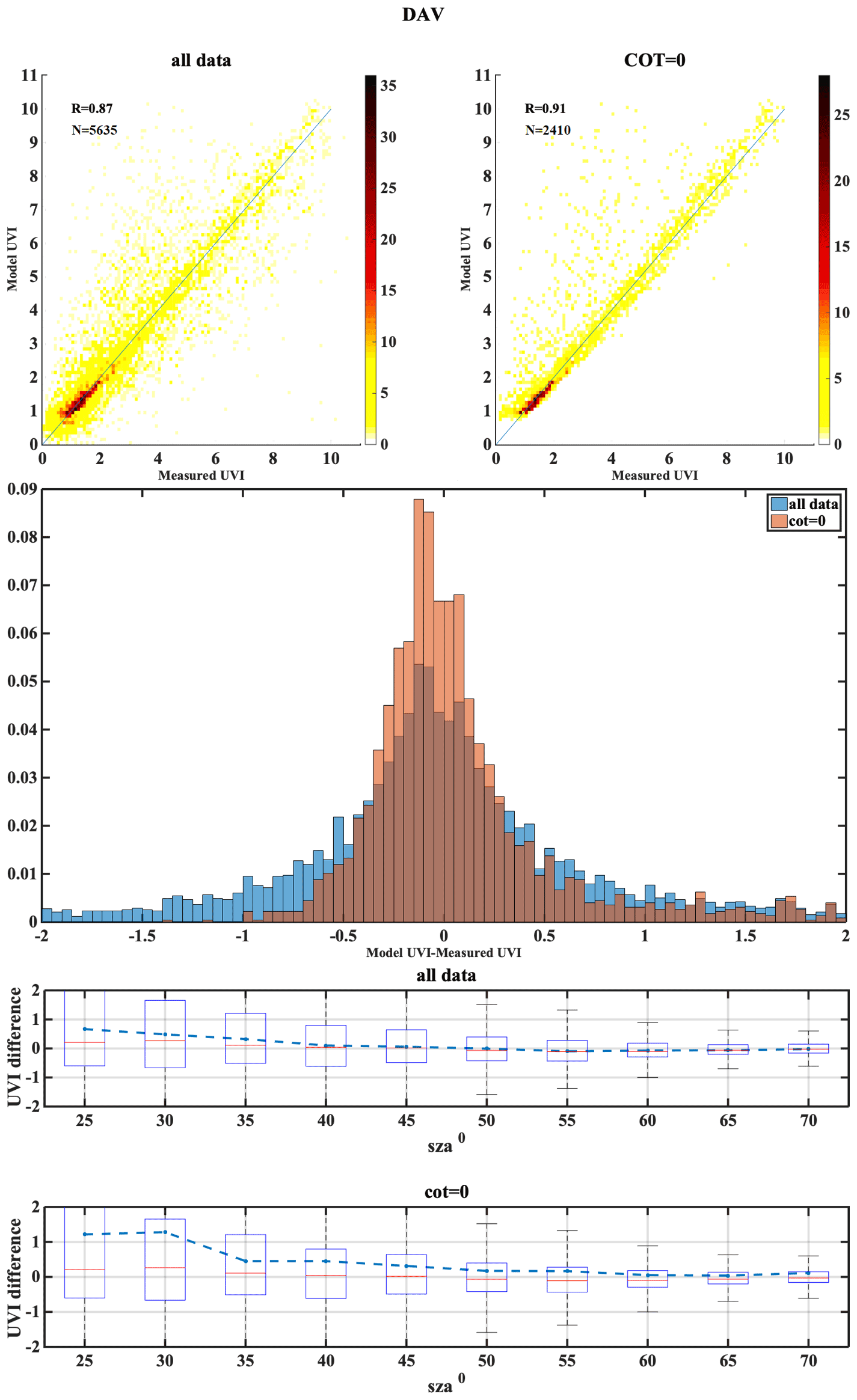
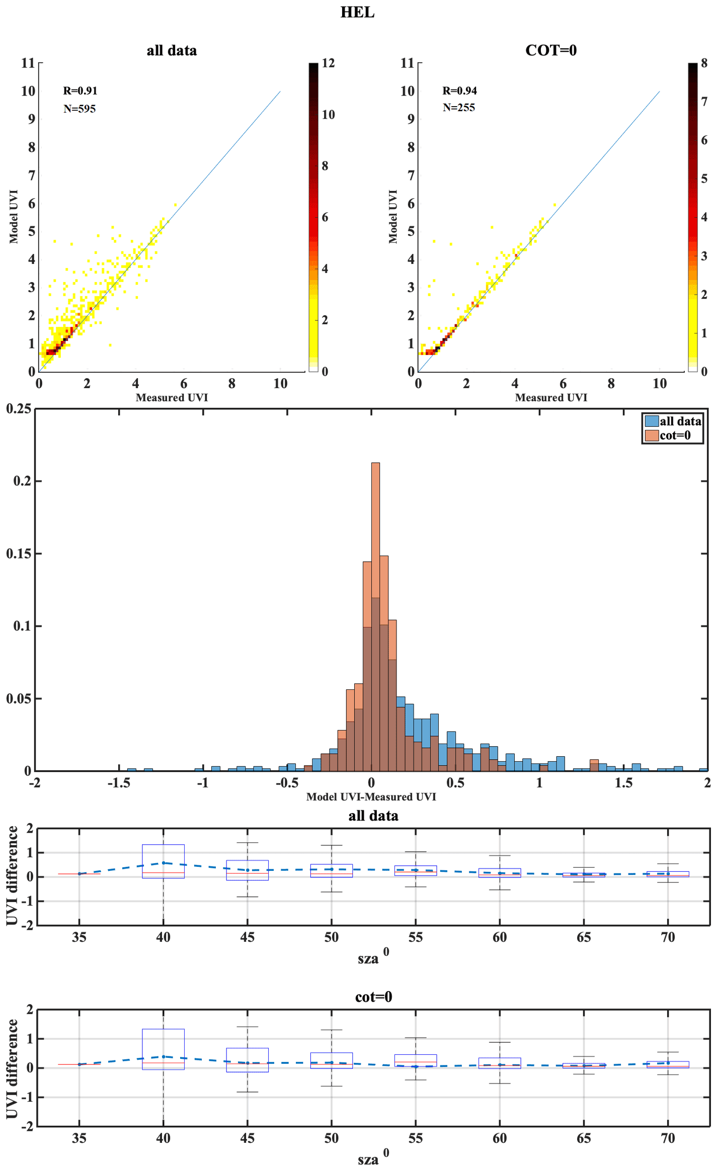
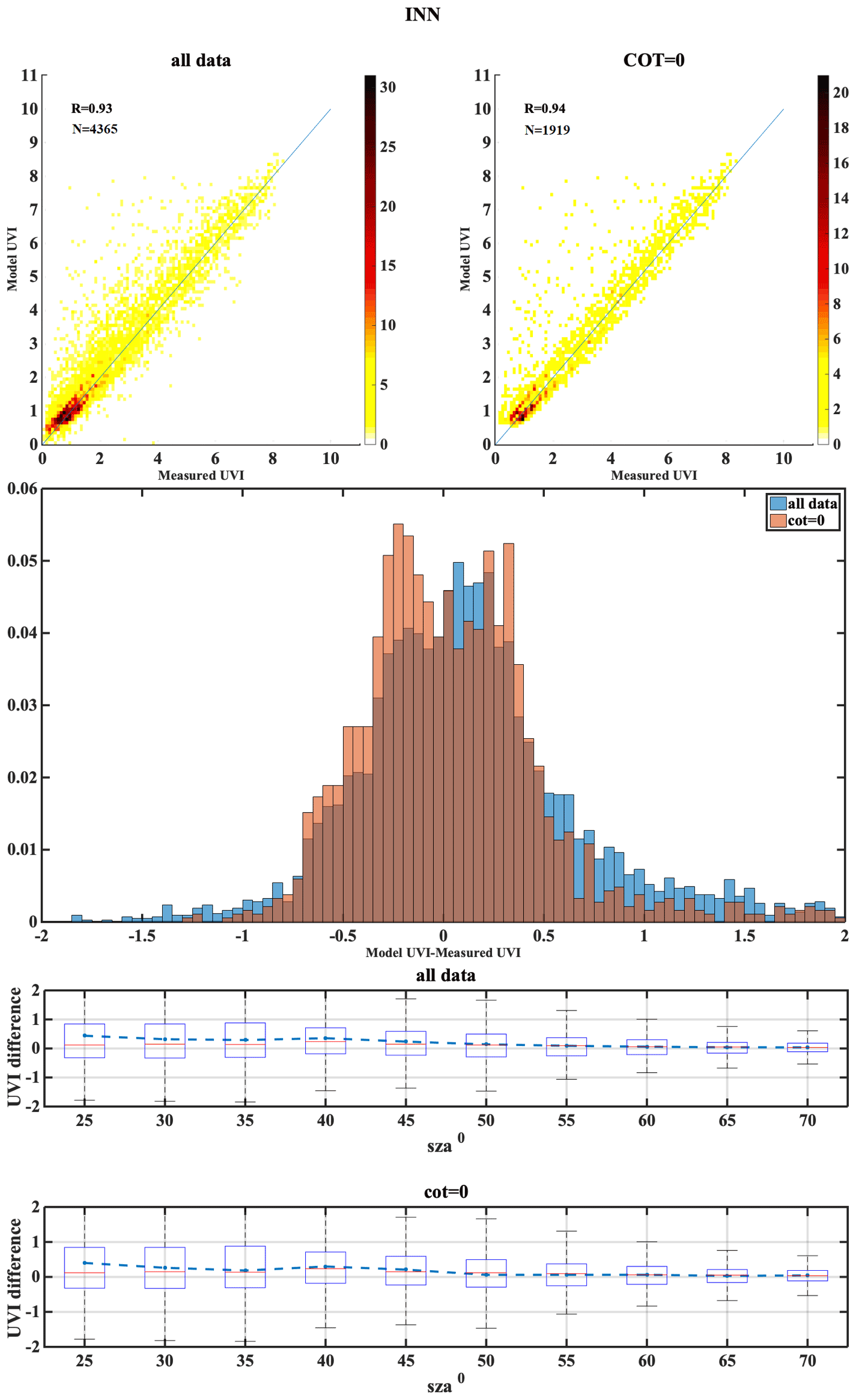
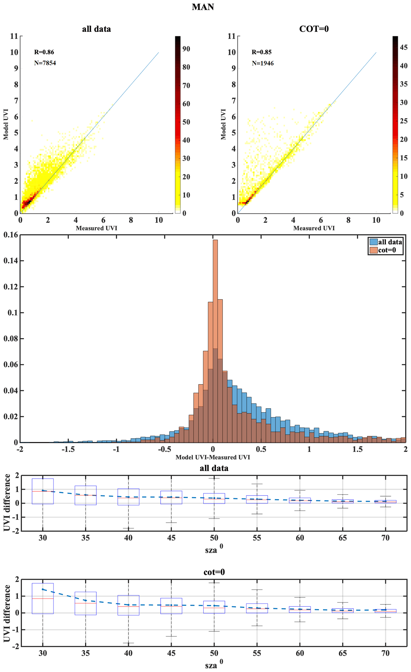
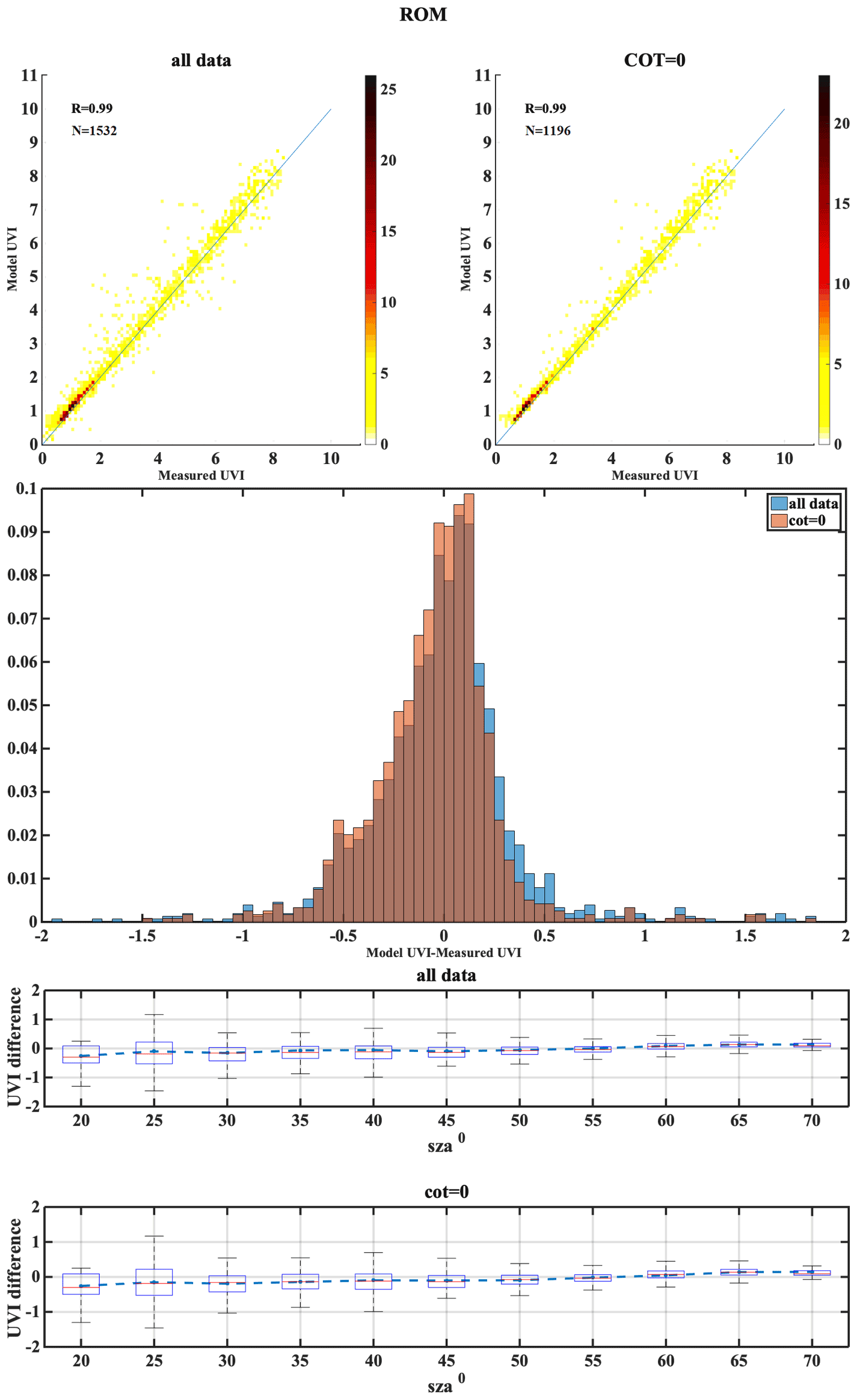
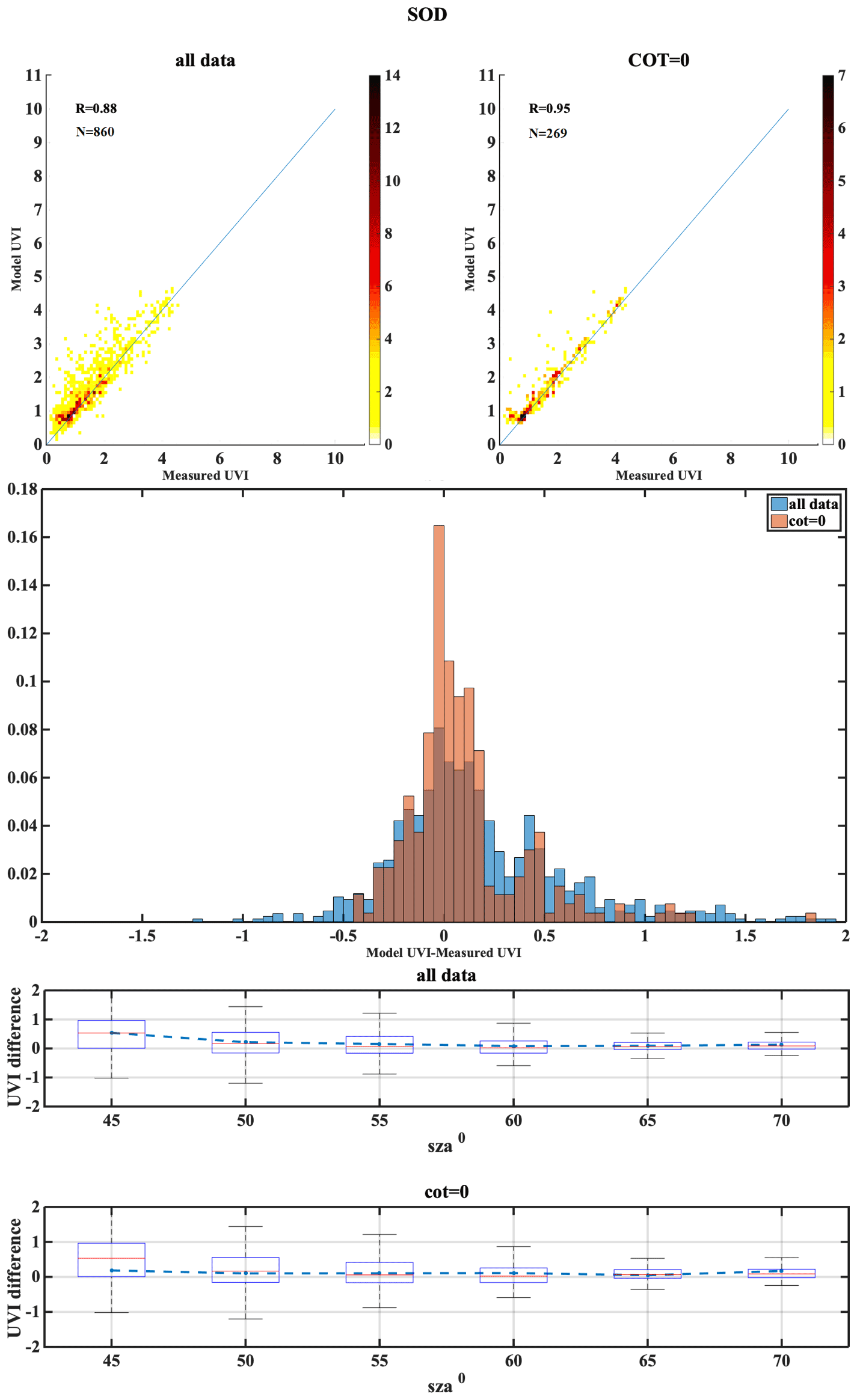
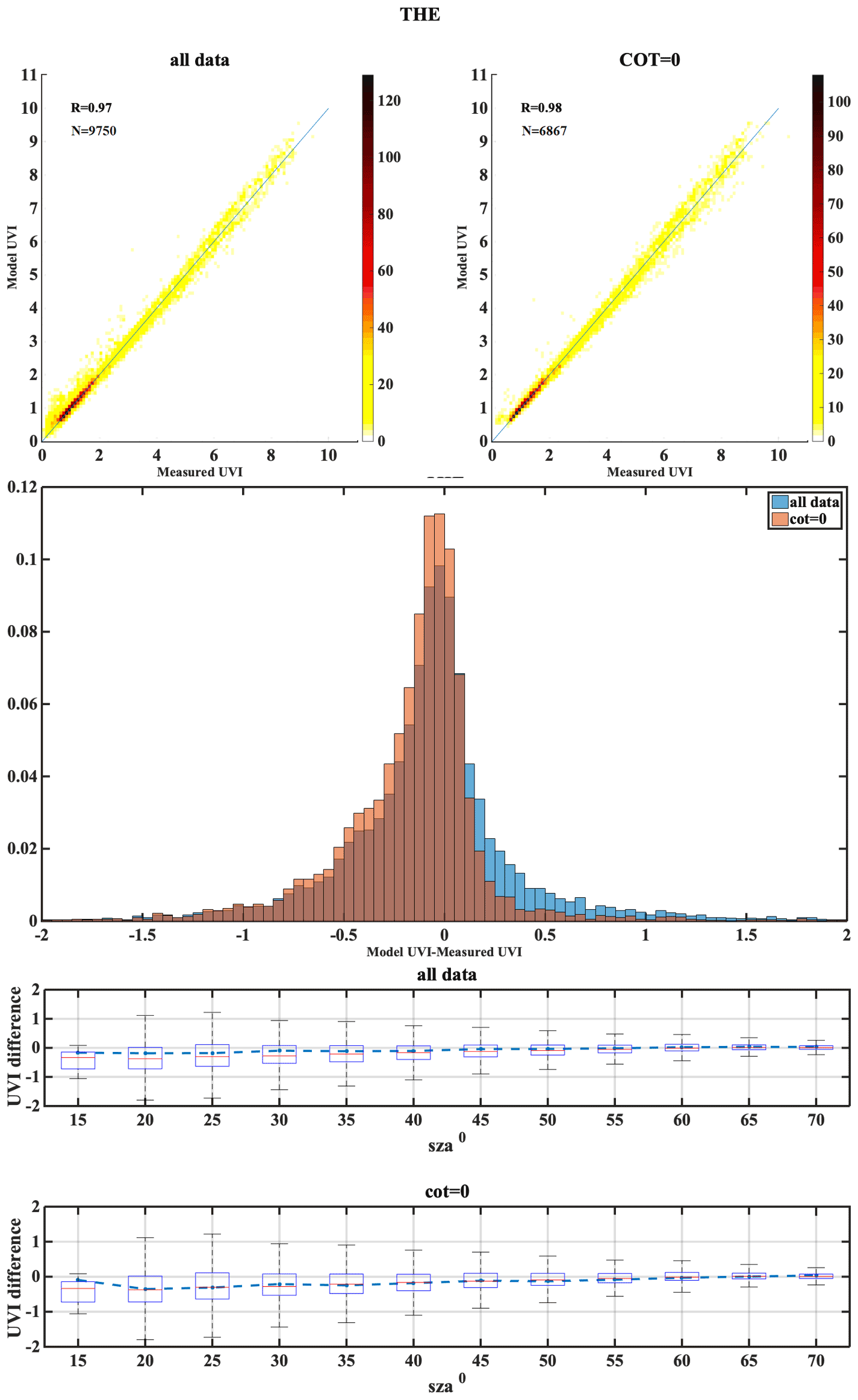
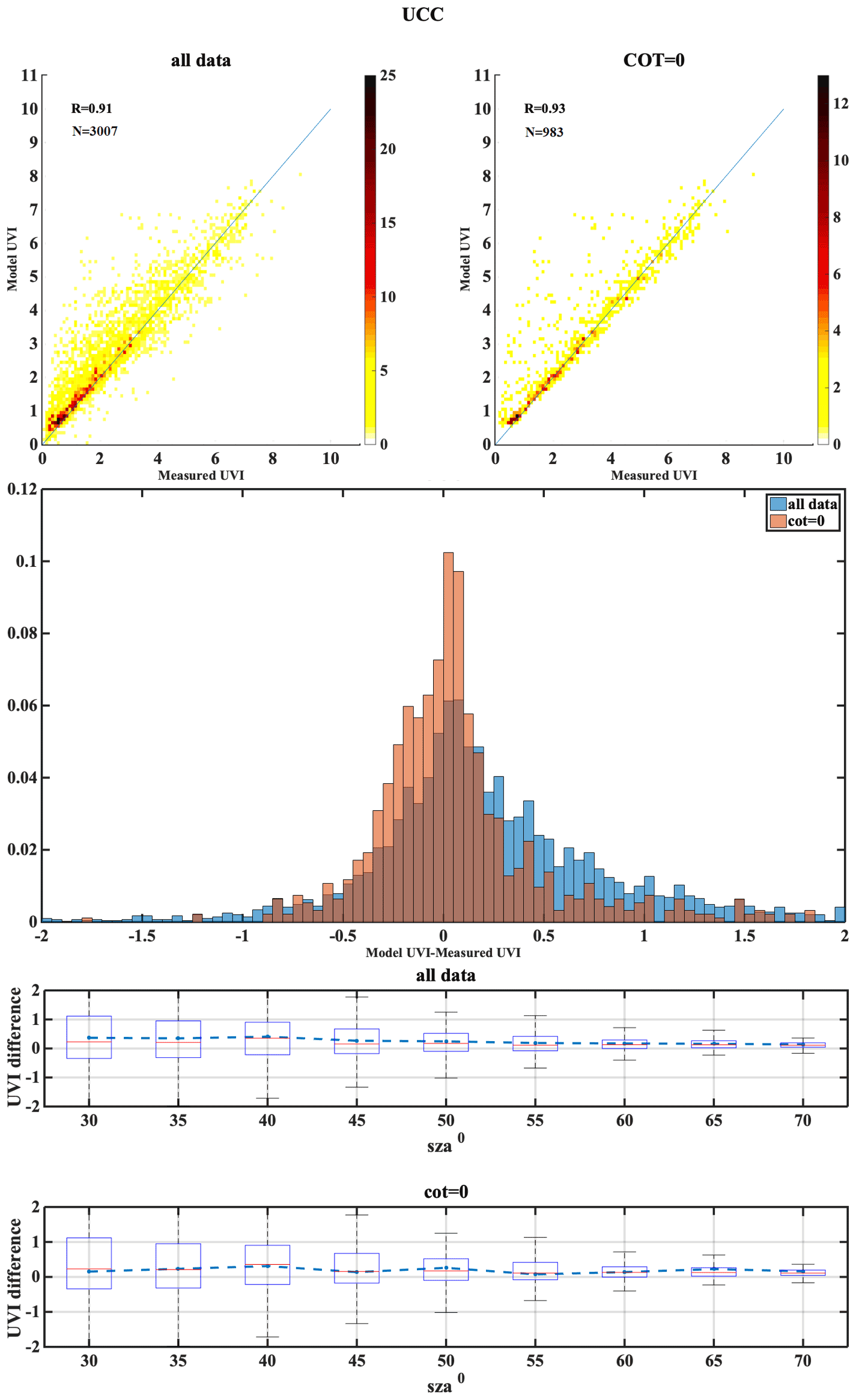
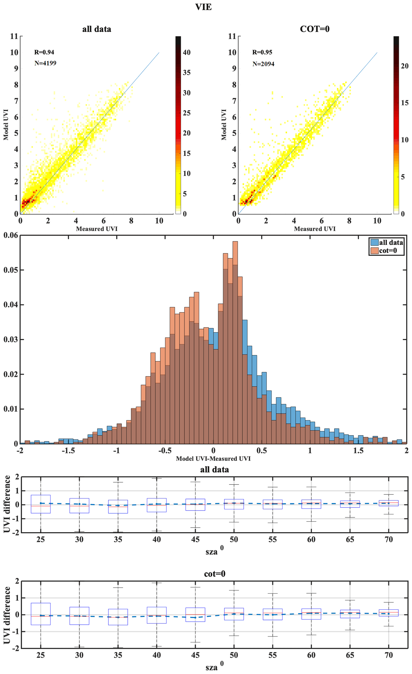
The following set of figures (Figs. A1–A17) shows for all stations, in the upper row, density scatterplots of measured and modeled UVI for all-sky and clear-sky conditions, followed by the correlation coefficient (R) and the number of data points (N) used in the analysis. In the middle row, the normalized probability histogram of differences is depicted, while the lower row presents the boxplot of differences as a function of SZA, representing median (red lines), mean (blue dotted lines), 25th–75th percentiles (blue boxes) and 5th–95th whiskers (dotted lines).

We have categorized the stations mostly based on cloud cover as Mediterranean, central Europe, high altitude and high latitude. Each of the stations has its own characteristics in terms of atmospheric conditions and parameters affecting the UVI reaching the ground. A summary of the results with possible explanation of the differences observed are shown here. The Mediterranean region includes the stations THE, ATH, AKR, ROM, VAL and ARE. Analysis of TOC showed that in most of the cases UVI mean differences are less than 0.1 in general, while a negative bias between TOC and the ground measurements was seen to be highest for ROM (−9.9), which corresponds to the UVI difference of 0.3. The impact of AOD uncertainty showed the correlation coefficient between the modeled and measured UVI values above 0.7 for most of the stations, while it was as high as 0.91 for ARE. The mean bias between the modeled and measured UVI for the clear-sky condition was found to be less than that for the all-sky condition for the stations AKR, ATH and THE that had most days of the year as cloud-free (the clear-sky percentage is above 70 %). The mean bias between the modeled and measured UVI for the clear-sky condition was more than the all-sky condition for ARE, even though it had mostly clear skies throughout the year. The analysis of the combined effect of the aerosol and ozone at Thessaloniki revealed that the model showed a slight underestimation with real inputs (AERONET and Brewer) but overestimations for forecasted inputs (CAMS and TEMIS). However, the coefficient of correlation was found to be 0.989 and 0.992 for the model with forecasted and real inputs, respectively. Stations of this classification have the single scattering albedo ranging from 0.76 to 0.93, with most of them having SSA values between 0.83 and 0.93, except stations ARE and THE, which had relatively smaller SSA values (0.76–0.9) and greater variability and large MBE. AKR station comparison showed that some UVIOS calculated UVI at higher levels than the ground-based measurements, especially at low SZAs. However, ground-based UVI measurements seem more unrealistic than the UVIOS-calculated UVI for summer local noon conditions as modeled UVIs with real AOD and TOC measurements in the area tend to agree with UVIOS outputs.

The second classification is the central European regions, including AOS, UCC, BEL, MAN, LIN, VIE and INN. The median of the absolute UVI differences between the model and the measurement for the all-sky condition were higher for MAN and UCC, while for others it was close to zero. Larger UVI difference of −0.22 due to the TOC uncertainty impact was observed for AOS, which might be due to large values of UVI at higher altitudes, as the positive bias is highest for the AOS station (7.6). The UVIOS MBE and RMSE statistical scores for analyzing the AOD uncertainty impact showed a mean positive bias up to 0.071 for all the stations except UCC, which showed a mean negative bias of 0.007. The mean bias between the modeled and measured UVI for the clear-sky condition was more than the all-sky condition for AOS even though it had mostly clear skies throughout the year. BEL, UCC and VIE showed more MBE for the clear-sky condition than the all-sky condition as they have mostly cloudy skies throughout the year (clear-sky annual percentage less than 50 %). However, stations LIN and MAN also have more MBE for the clear-sky condition even though they have most days of the year as cloudy (clear-sky annual percentage less than 45 %). Analysis of AOD uncertainty showed that the UVI difference was highest for VIE than the other stations. The monthly values of the single scattering albedo used in UVIOS ranged from 0.76 to 0.93 for stations AOS, UCC and MAN, with most of them having SSA values between 0.83 and 0.93 and relatively small variability, while the stations BEL, INN, LIN and VIE had relatively smaller SSA values (0.76–0.9) and greater variability than the other stations, and most of these stations have shown large MBE.

The high-altitude station is DAV and high-latitude stations include LAN, HEL and SOD. DAV have less MBE for clear-sky conditions even though they have most days of the year as cloudy (clear-sky annual percentage less than 45 %). DAV and MAN show worse statistical behavior for clear sky, which is probably caused by misclassification of cloudy pixels. For DAV this could be explained by the complex mountainous topography of the area. Large UVI differences in SOD and HEL indicate higher introduced uncertainties over higher latitudes. Higher aerosol levels in the atmosphere tend to lower the UVI. Highest difference in UVI is observed for the stations HEL, SOD and VIE. Since, the aerosol level at the stations HEL and SOD is very low this leads to higher UVI which can be the reason for the small UVI differences observed for these stations. The stations of this classification have mostly cloudy skies throughout the year (clear-sky annual percentage less than 50 %) and have more MBE for the clear-sky condition than the all-sky condition. This might be due the fact that the clouds are not captured well at a point station and a cloudy sky might have been considered as a clear sky. Higher UVI difference was observed for HEL and SOD as a result of AOD uncertainty analysis which might be due to the low aerosol content of these stations due to higher latitude that leads to higher UVI values.

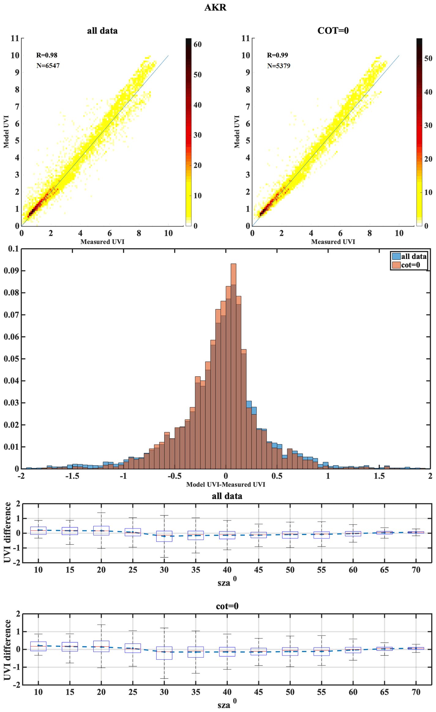
Figure A1 Density scatterplots of measured and modeled UVI for all-sky and clear-sky conditions (upper row) for the AKR station, normalized probability histogram of differences (middle row) and boxplot of differences as a function of SZA (lower row).

Figure A2 Same as above but for the AOS station.

Figure A3 Same as above but for the ARE station.

Figure A4 Same as above but for the ATH station.

Figure A5 Same as above but for the BEL station.

Figure A6 Same as above but for the DAV station.

Figure A7 Same as above but for the HEL station.

Figure A8 Same as above but for the INN station.

Figure A9 Same as above but for the LAN station.

Figure A10 Same as above but for the LIN station.

Figure A11 Same as above but for the MAN station.

Figure A12 Same as above but for the ROM station.

Figure A13 Same as above but for the SOD station.

Figure A14 Same as above but for the THE station.

Figure A15 Same as above but for the UCC station.

Figure A16 Same as above but for the VAL station.

Figure A17 Same as above but for the VIE station.