the Creative Commons Attribution 4.0 License.
the Creative Commons Attribution 4.0 License.
 | 26 Aug 2021
SIBaR: a new method for background quantification and removal from mobile air pollution measurements
Blake Actkinson
Katherine Ensor
Robert J. Griffin
Mobile monitoring is becoming increasingly popular for characterizing air pollution on fine spatial scales. In identifying local source contributions to measured pollutant concentrations, the detection and quantification of background are key steps in many mobile monitoring studies, but the methodology to do so requires further development to improve replicability. Here we discuss a new method for quantifying and removing background in mobile monitoring studies, State-Informed Background Removal (SIBaR). The method employs hidden Markov models (HMMs), a popular modeling technique that detects regime changes in time series. We discuss the development of SIBaR and assess its performance on an external dataset. We find 83 % agreement between the predictions made by SIBaR and the predetermined allocation of background and non-background data points. We then assess its application to a dataset collected in Houston by mapping the fraction of points designated as background and comparing source contributions to those derived using other published background detection and removal techniques. The presented results suggest that the SIBaR-modeled source contributions contain source influences left undetected by other techniques, but that they are prone to unrealistic source contribution estimates when they extrapolate. Results suggest that SIBaR could serve as a framework for improved background quantification and removal in future mobile monitoring studies while ensuring that cases of extrapolation are appropriately addressed.
- Article
(7327 KB) - Full-text XML
-
Supplement
(6421 KB) - BibTeX
- EndNote


Understanding air pollution exposure is important, as it has been linked to various adverse health conditions (Caplin et al., 2019; Zhang et al., 2018). Mobile monitoring, a technique in which continuous air pollution measurements are collected using instrumentation on a mobile platform, is becoming increasingly important for characterizing exposure because air pollution varies on spatial scales finer than the typical distance between stationary monitors (Apte et al., 2017; Chambliss et al., 2020; Messier et al., 2018).
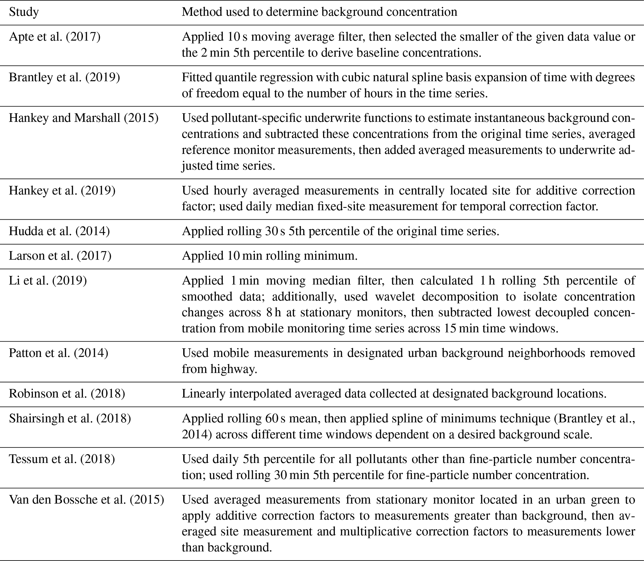
A key component of mobile monitoring analysis is identifying ambient background levels, defined here as measured air pollution concentrations independent of local source influences (Brantley et al., 2014). Background quantification is vital from both policy and exposure perspectives, as it is important to assess the contribution of local sources to pollution concentrations accurately. Table 1 summarizes the wide variety of methods used to estimate background in studies incorporating mobile monitoring published within the past 5 years. The wide variance in the approaches used is problematic, as estimates of source contributions to measurements have been shown to be sensitive to the technique used (Brantley et al., 2014). To improve the replicability and power of mobile monitoring studies, a more consistent technique for background estimation is needed.
Table 1Summary of previous methodologies for estimating background levels of air pollution in mobile monitoring campaigns.
Designing a method to determine the background in mobile monitoring studies presents several challenges. Measurements in remote locations are often regarded as the most reliable representation of background concentrations; however, remote locations may be inaccessible for some mobile monitoring studies and are themselves subject to occasional source influences. These drawbacks make time series methods for determining background more desirable. However, many time-series-based methods often rely on setting static time windows, which are usually determined by the expected duration of influence from source plumes within the mobile monitoring study (Bukowiecki et al., 2002). The underlying physical representation of these time series methods remains unclear for more extensive mobile monitoring campaigns, as the setting of static time windows does not often capture the entire variation in timescales that source impacts can have on mobile measurements.
Here we show the results of a newly developed method called State-Informed Background Removal (SIBaR) used to estimate background for several traffic-related air pollutants, namely nitrogen oxides (NOx) and carbon dioxide (CO2). The method incorporates hidden Markov models (HMMs), a time series regime modeling technique used in a wide variety of contexts in signals processing, finance, and the social sciences and that has been used to model background in stationary monitors (Gómez-Losada et al., 2016, 2018, 2019; Visser and Speekenbrink, 2010). HMMs assume that observations within a time series are drawn from probability distributions governed by a hidden sequence of states. We propose decoding this hidden sequence of states as a way to determine whether measurements were taken during time periods representative of background versus time periods subject to local influences. We illustrate that a more physically meaningful representation of background is captured in this modeling context for mobile monitoring time series and show its application to a wide variety of traffic-related air pollutant measurements. As a proof of concept, we run the method on a published external dataset already marked as background and non-background and assess its performance. As a first application and to provide further proof of concept, we map points binned as background by SIBaR to show their spatial distributions. As a proof of importance, we highlight differences in mapped source contributions derived from SIBaR background and background derived from other time-series-based techniques. Results indicate that our consistent method for background identification and removal has a noticeable impact on mapped mobile source contributions.
2.1 Mobile campaign
Measurements were taken during the Houston Mobile Monitoring Google Street View (GSV) campaign and are described in detail elsewhere (Miller et al., 2020). Measurements were conducted over a 9 month period spanning July 2017 to March 2018. Sampling primarily took place between 07:00 and 16:00 local standard time (Miller et al., 2020) in a variety of census tracts across metropolitan Houston. Census tracts are included in the current analysis if they were sampled a minimum of 15 times during this 9-month period (Apte et al., 2017; Li et al., 2019). Details and names used to describe each census tract are given in Table S1 in the Supplement. The time of day and day of week for each census tract visit were predetermined to minimize temporal biases in sampling to the greatest extent possible. Instruments (Table S2) were loaded into two gasoline-powered GSV cars that sampled every drivable road in 22 different census tracts in the greater Houston area. Details and names used to describe each of the census tracts considered are given in Table S1. Individual observations are aggregated to 50 m points in neighborhoods and 90 m points on highways using a road network created from U.S. Census TIGER/Line roads (TIGER/Line Shapefile, 2018). More details on the road network creation and data quality control are provided elsewhere (Miller et al., 2020). Data quality and control measurements were implemented to ensure sound statistics were performed. Measurements were removed if they were taken during calibration periods, during periods of suspected instrument failure, and if they were outside of an instrument's reported operating range. Measurements were synchronized to GPS time stamps and adjusted for inlet residence time differences based on results from match strike tests. Measured pollutants include black carbon (BC), carbon dioxide (CO2), nitric oxide (NO), and nitrogen dioxide (NO2) (NOx = NO + NO2).
Bias, precision, and the minimum detection limit (MDL) for each instrument are provided in Table S2. Details concerning the calculation of each parameter for each instrument are given elsewhere (Miller et al., 2020). In brief, the bias for the T200 NO analyzer and T500U NO2 analyzer were calculated from gas calibration checks performed every 2 weeks at the start of the study period and every month towards the end of the study period because the checks routinely showed bias 10 %. The bias for the LI-7000 CO2/H2O Analyzer was determined from a gas phase calibration before the start of the study to match the manufacturer reported value. Precision values for the T200 and T500U were calculated as the standard deviation of zeroing periods taken throughout the entire campaign. Minimum detection limits for the T200 and T500U were determined as the mean of the time series zero +3σ. The minimum detection limit and precision of the Li-COR were not considered due to taking measurements at a consistently elevated global background and the latter manufacturer's reported value having a minuscule effect on the overall uncertainty of the measurement. For the purposes of this work, we perform no MDL substitution, as MDL substitution would censor the underlying modeled background probability distribution.
2.2 Hidden Markov model categorization – the background partitioning step
Time series observations are segregated by day and for each GSV car, and HMMs are fit to each day's worth of data. Before fitting the HMM to each day's time series realizations, we log transform them. HMMs attempt to maximize the log-likelihood, LC, determined by the sum of the forward variables αT(i):
in which i designates state i (total states N) at the last realization of the time series T. The forward variables are derived recursively as
in which πi represents the initial probability for state i, aij represents the state transition probability from state i to state j, and p(yt|θi,z) represents the conditional probability of observation yt conditioned on the parameters θi governed by state i and any additional covariates z. For the purposes of our work, we assume that the probability distributions governing yt are log normal and parametrize the mean of the response distribution as
where μt is the time-dependent mean of the response, and are estimated parameters, and t is time.
The log-likelihood of Eq. (1) is maximized using the expectation maximization algorithm (Dempster et al., 1977; Visser and Speekenbrink, 2010). Initial starting values of the transition probabilities are bootstrapped 150 times to produce 150 candidate models because convergence to a maximum likelihood can be affected by the starting values. The model with the greatest log-likelihood is then selected for decoding via the Viterbi algorithm (Forney, 1973). The Viterbi algorithm seeks to maximize the joint probability of both observations and state sequence () given the parameters. We define a variable δ recursively as
with the initialization
To retrieve the state sequence, we create a matrix ψ such that
We retrieve the state sequence by backtracking:
This state sequence is then used to designate observations as background or source. State-assigned points with the lower median are designated background. An example of a decoded sequence is given in Fig. 1 for NOx (after retransformation).
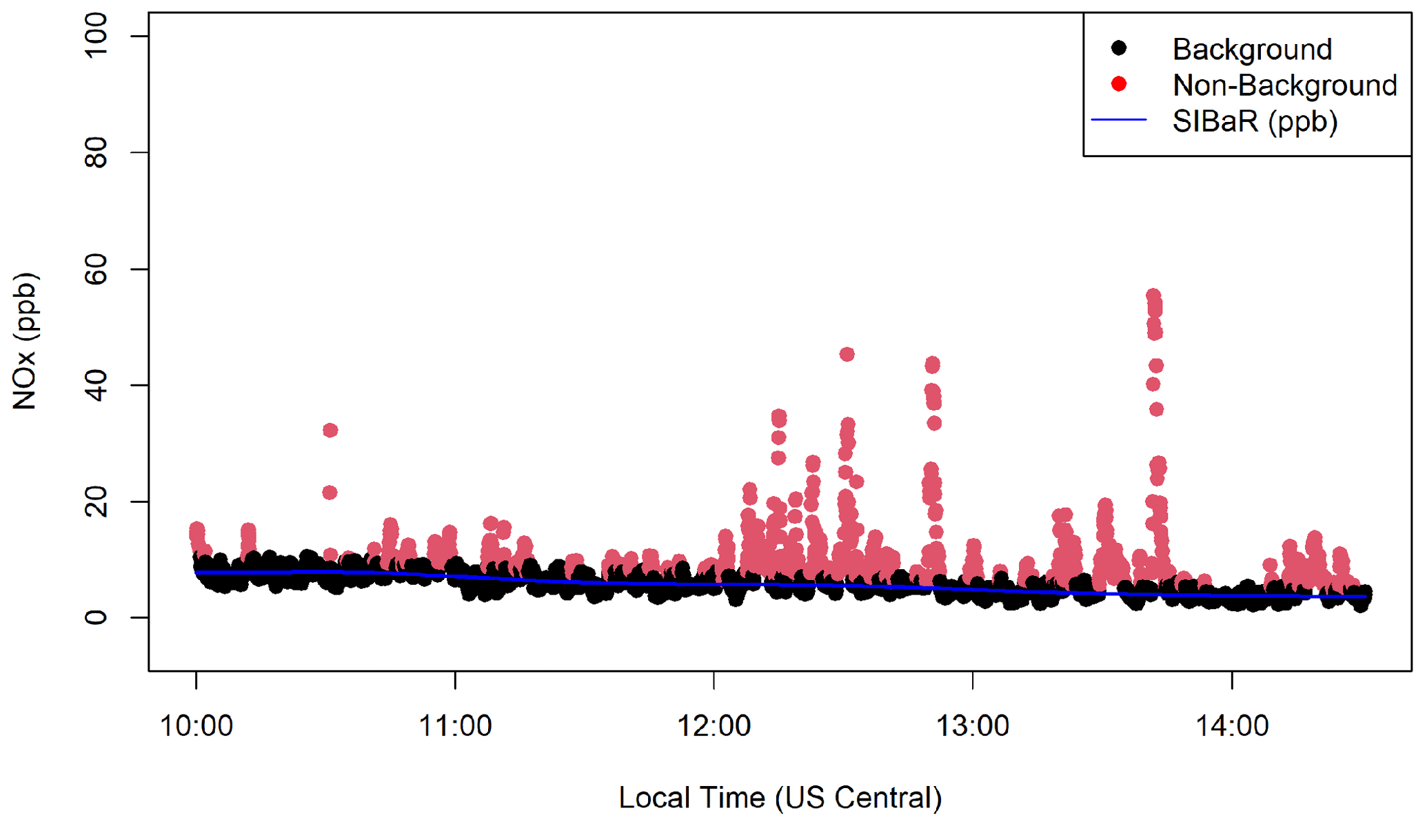
Figure 1Example time series of SIBaR background signal (blue) being fit to background designated points (black) created in the SIBaR partitioning step. Points are colored red if designated as the source in the partitioning step and black if designated background. Data presented in this time series were collected on 30 March 2018 starting at 10:00 Central Daylight Time (CDT).
HMM fits can be highly sensitive to time series outliers (Svensén and Bishop, 2005; Chatzis and Varvarigou, 2007; Chatzis et al., 2009). Additionally, while computationally cheap, the linearity assumption embedded in the time covariate could fail to capture more complex variations in background and produce flawed state categorizations. To capture misclassification instances, we recast the step as an unsupervised learning problem, design an empirical routine to evaluate the quality of created clusters, and incorporate it into SIBaR. The routine, coined the fitted line classifier, fits a line between averaged transition measurements and their corresponding transition times. The method then calculates the percentage of points above the line that are classified as background and the percentage of points below the line that are classified as source. If either percentage is greater than or equal to 50 %, a predetermined percentage threshold, the method deems the series incorrectly classified. If a series is incorrectly classified, SIBaR breaks the series into two and performs the background partitioning step on each half chunk separately. Sixteen example time series, labeled as classified correctly or incorrectly, are depicted in Figs. S1 and S2. After fitting HMMs to each separate chunk, SIBaR then uses the fitted line classifier on each chunk, repeating the process if any chunk's partitioning is labeled misclassified. The process continues recursively until all created partitions are deemed correctly classified. SIBaR then combines the state designations from all created chunks into one and returns those state designations as the corrected designations for the time series.
In running SIBaR on the campaign NOx measurements, we note that the empirical classifier designates 96 % of the original time series to be correctly classified for a 50 % threshold. We run a sensitivity analysis on the percentage threshold and show the results in Fig. S3. The figure illustrates that changing the percentage threshold causes changes in the percentage of correctly classified time series to range between 80 %–100 %, dipping below 50 % only for the most stringent requirement (5 %). These results give us confidence in the partitioning step.
2.3 Natural spline fit
After HMMs have been fit to all time series data, natural splines are fit to the background points by day. As in the work published by Brantley et al. (2019; “Brantley”), we select a natural spline basis with the degrees of freedom equal to the number of hours in the time series. However, we fit to the mean of our partitioned background time series, whereas in Brantley the focus is on a 10th quantile regression. An example of this spline fit is given in Fig. 1.
Because SIBaR's partitioning step periodically generates background-assigned points that differ from one another for the same time series, we perform a test to evaluate its robustness. We run SIBaR 25 times and evaluate the pairwise root mean square error (RMSE) between each set of generated background predictions for NOx as defined by
in which nta is the background realization at time t of signal a, ntb is the background realization at time t of signal b, and T is the total number of realizations in the time series.
The pairwise RMSE values for the first 12 runs are given in Table S3. We calculate an average RMSE of 0.05 ± 0.02 ppb between each background signal and conclude that the fitting step is robust to small changes in background-assigned points in the partitioning step.
2.4 Evaluating the partitioning step: validation on an external dataset
To test the validity of the partitioning step, we perform external validation using a mobile monitoring dataset published in Brantley et al. (2014). In that study, a van collecting mobile measurements of carbon monoxide (CO) systematically looped a route in which it drove through a predefined background location, on transects to a highway, and on the highway itself (Brantley et al., 2014). The measurements taken in the prescribed background location were marked as background, and all other measurements were marked as non-background. We run the partitioning step on these data to determine how well SIBaR captures the measurements taken in the background location of the study.
2.5 Generating mapped fractional background contribution and source contribution maps
We explore the spatial extent of our HMM-decoded categorizations from the partitioning step by creating mapped fractional background contribution maps. After aggregating time series observations (either CO2 or NOx, depending on the pollutant analyzed) to road segment points created within our road segment network, we sum the number of observations designated as the background state and divide by the total number of observations assigned to that road segment point. We map the results and present them in Sect. 3.2.
In Sect. 3.3, we derive source contributions (source signal = original signal – background signal) using our background method and map them. To put these source contributions in context with previously published work, we repeat the same process using background derived from a moving 2 min 5th percentile baseline (Apte et al., 2017; “Apte”) and the Brantley technique described previously in Sect. 2.2 (Brantley et al., 2019). To derive our source contributions, we make predictions for the background for each time series realization collected using the derived background spline and then subtract those predictions from the original time series observations. We also derive source contributions using the Apte and Brantley techniques. We create the maps using the same methodology as Miller et al. (2020) and described briefly here. Using our created road segment network, we take the mean of measurements collected as the GSV car drives past a road segment point in our network, coined the drive pass mean. We take the median of these drive pass means and map the result. Because we consider drive pass means taken within 4 h of one another to provide no new information about the air quality at that road segment, we take the median of drive pass means occurring within that 4 h time window to generate a 4 h median of drive pass means. Then, we take the median of all 4 h medians of drive pass means at that road segment to derive its map-reduced median. We perform this procedure for the source contributions derived using our method and the source contributions derived using the other published methods.
3.1 Validating the partitioning step on an external dataset
A comparison between SIBaR's partitioning and the partitioning originally published by Brantley et al. (2014) is given in Fig. 2. Initially, the HMM fitting step is performed and the resulting state sequence decoded. We run our classifier on the initially decoded time series and find it to be misclassified, which is apparent from panel (a) of Fig. S4, which shows the unsmoothed CO data before correction. The algorithm breaks the series into two chunks and refits the HMM to each part separately, resulting in the state designations in panel (a) of Fig. 2. We then compute the percentage of matching background/non-background designations. The SIBaR partitioning step is able to match 83 % of the originally published background/non-background designations. The mismatches could be attributed to the transition between the background/non-background portions of the route in the original study, which is observed in Fig. 2 in the periods where background points show larger values than source points near periods of the transition (for example, the last blue spike at approximately 08:45 Eastern Daylight Time, EDT). Mismatches also could be a result of the effects of traffic on measurements in the background designated portion of the route. Finally, the mismatches could be attributed to the inability of the SIBaR linearity assumption to capture finer scale temporal variations within the background (see Eqs. 2–4).
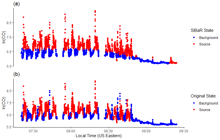
Figure 2Comparison between SIBaR-predicted background and source states and originally published designations from Brantley et al. (2014) for log-transformed CO. Background designated points are in blue and source designated points in red. (a) SIBaR-decoded states for the mobile CO measurements. (b) Designations originally published by the authors of the study.
In running this test, we note that the method is sensitive to a smoothing time window if one is used. Figure S4 illustrates uncorrected SIBaR-decoded states for three different smoothing time windows on the same CO dataset and shows that the method produces different state categorizations depending on the window used, even making correction unnecessary in the 30 s instance. We hypothesize that smoothing reduces the skewness of the data such that they better fit two switched lognormal Gaussian distributions.
3.2 Mapped fractional background state contributions
For the Houston mobile campaign, maps detailing the fractional contribution of the background state to the overall mapped points are created for CO2 and NOx. Individual observations assigned to a road segment point have their decoded category designations assigned to the same point. The number of observations assigned the background category are then divided by the total number of observations assigned to the point to determine the fractional background state contribution. Figure 3 shows these census tract maps for NOx. Figure S5 shows the maps for CO2. It is important to note that these maps represent the fraction of the measurements that are categorized as background or source for the given pollutant at a given location.
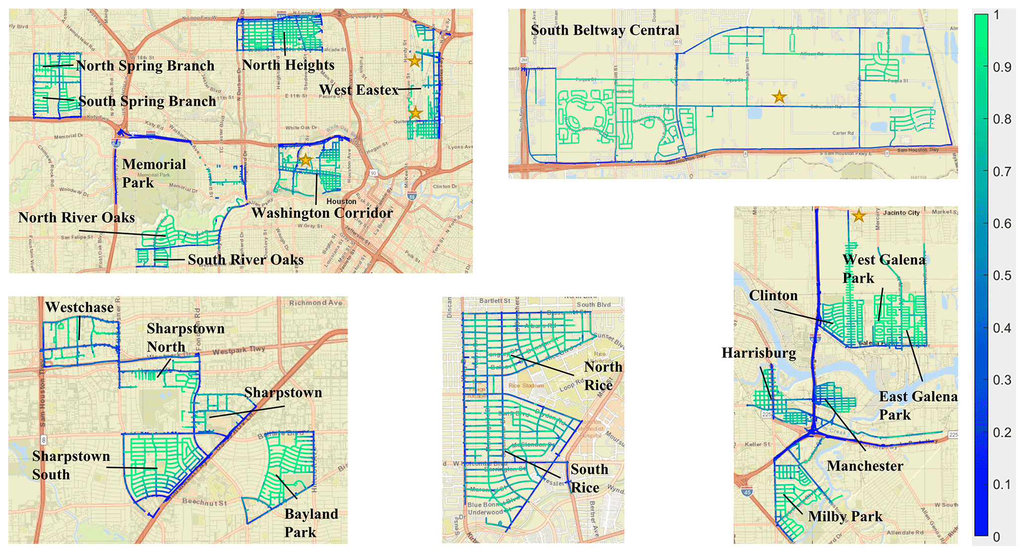
Figure 3Fraction of points aggregated to the road segment network designated as background in SIBaR-decoded states for NOx. Maps were generated following the methods outlined in Sect. 2.5. Points are mapped on a scale of 0 to 1; 1 implies all points aggregated to that road segment were designated as background and 0 implies all points were designated as non-background. Details of the census tracts are provided in Table S1. Gold stars indicate locations of elevated NO and/or NO2 medians next to known industrial facilities published in Miller et al. (2020). Basemap generated by MATLAB geobasemap “streets” and is hosted by ESRI (Sources: Esri, DeLorme, HERE, USGS, Intermap, iPC, NRCAN, Esri Japan, METI, Esri China (Hong Kong), Esri (Thailand), MapmyIndia, Tomtom).
We note the following about the broad spatial patterns in the mapped background state fraction presented in Fig. 3. First, background state designated points dominate residential areas for both pollutants. This is encouraging, as it is expected that few point sources of these two pollutants would be found in residential neighborhoods except for those near industrial activity (Miller et al., 2020). Second, source state designated points dominate highways and busy arterial roads, which is expected given the large amounts of traffic on these roads. Finally, we note the appearance of source-dominated hotspots in front of point sources identified in our previous work (Miller et al., 2020) and denote their locations in Fig. 3. This is encouraging given that we found these road segments to be elevated for NO and/or NO2 compared to their surrounding neighborhood domain.
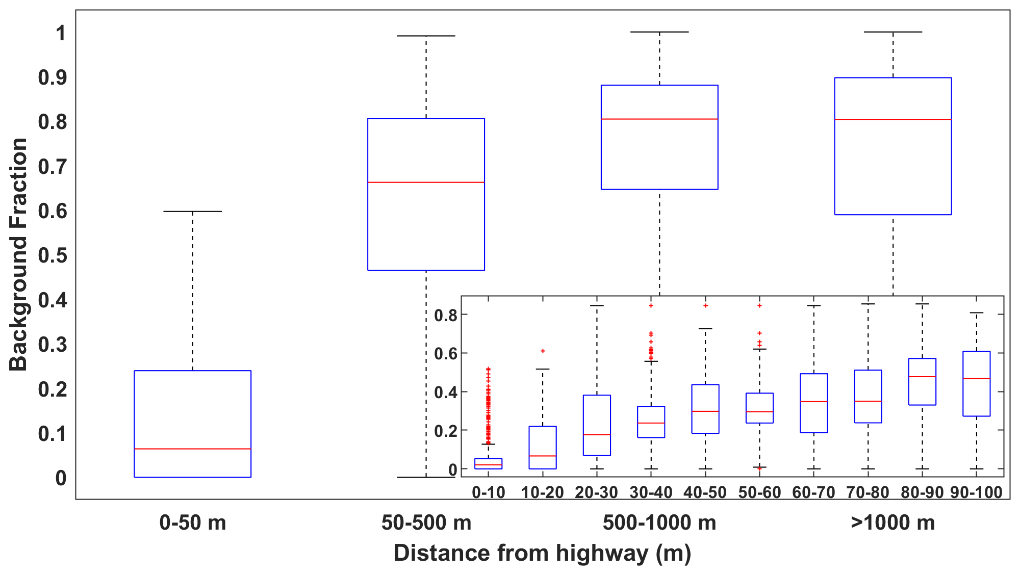
Figure 4Boxplots of mapped background NOx fractions, presented in Fig. 3, binned by distance from the highway. The red line represents the median, the top and bottom edges represent the 75th and 25th percentiles, respectively, and the whiskers extend to the most extreme data points not considered outliers.
We take the background state fractions depicted in Fig. 3 and bin them by distance to the highway. The results are presented in Fig. 4. We do the same for CO2 and present the results in Figs. S5–S6. The exponential behavior exhibited in Fig. 4 mirrors published exponential decays in roadside source pollutant concentrations (Apte et al., 2017; Karner et al., 2010), while the sizable interquartile ranges within each bin highlight the complexity and variability of source roadside gradients, which depend on emission rates, meteorology, geography, and other factors (Baldwin et al., 2015; Patton et al., 2014).
3.3 Comparison of source contribution maps using different background removal techniques
To put SIBaR predicted source contributions in context, we compare the source contribution maps generated using SIBaR to the ones generated by the Apte and Brantley techniques. We zoom in on the Ship Channel domain for ease of comparison in Fig. 5. We refer the reader to Figs. S7–S15 to see maps for all other areas in the mobile monitoring campaign for both NOx and CO2. The average NOx background predicted by the Apte, Brantley, and SIBaR techniques are 15.25, 11.58, and 13.02 ppb, respectively.
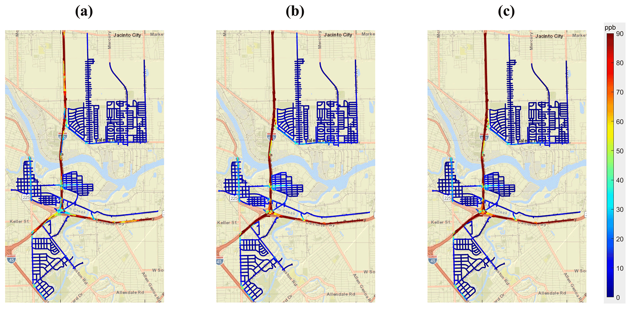
Figure 5Comparison of source contributions derived using different techniques in the Ship Channel domain. Source contributions were aggregated according to the methods described in Sect. 2.4. (a) Source contributions derived using the Apte technique. (b) Source contributions derived using the Brantley technique. (c) Source contributions derived using the SIBaR technique. Basemap generated by MATLAB geobasemap “streets” and is hosted by ESRI (Sources: Esri, DeLorme, HERE, USGS, Intermap, iPC, NRCAN, Esri Japan, METI, Esri China (Hong Kong), Esri (Thailand), MapmyIndia, Tomtom).
Figure 5 shows that the source contributions derived using the Apte technique are lower on highways compared to the source contributions derived using SIBaR and the Brantley techniques. Additionally, both the Brantley and SIBaR techniques derive higher source contributions on road segments with elevated NO and NO2 concentrations compared to the Apte technique, as identified in Miller et al. (2020). We hypothesize that this occurs due to the smaller time window utilized in the Apte technique. The GSV vehicles would often sit in traffic on highways for extended periods of time, making a 2 min time window unsuitable for describing source durations during those time periods. While the 2 min assumption would be better suited for situations in which the car was exposed to source durations within that time interval (which occurred in the Apte study), it would not be for source durations of a larger time interval, highlighting the challenges in assuming a static time window for extensive mobile monitoring campaigns with varying source durations.
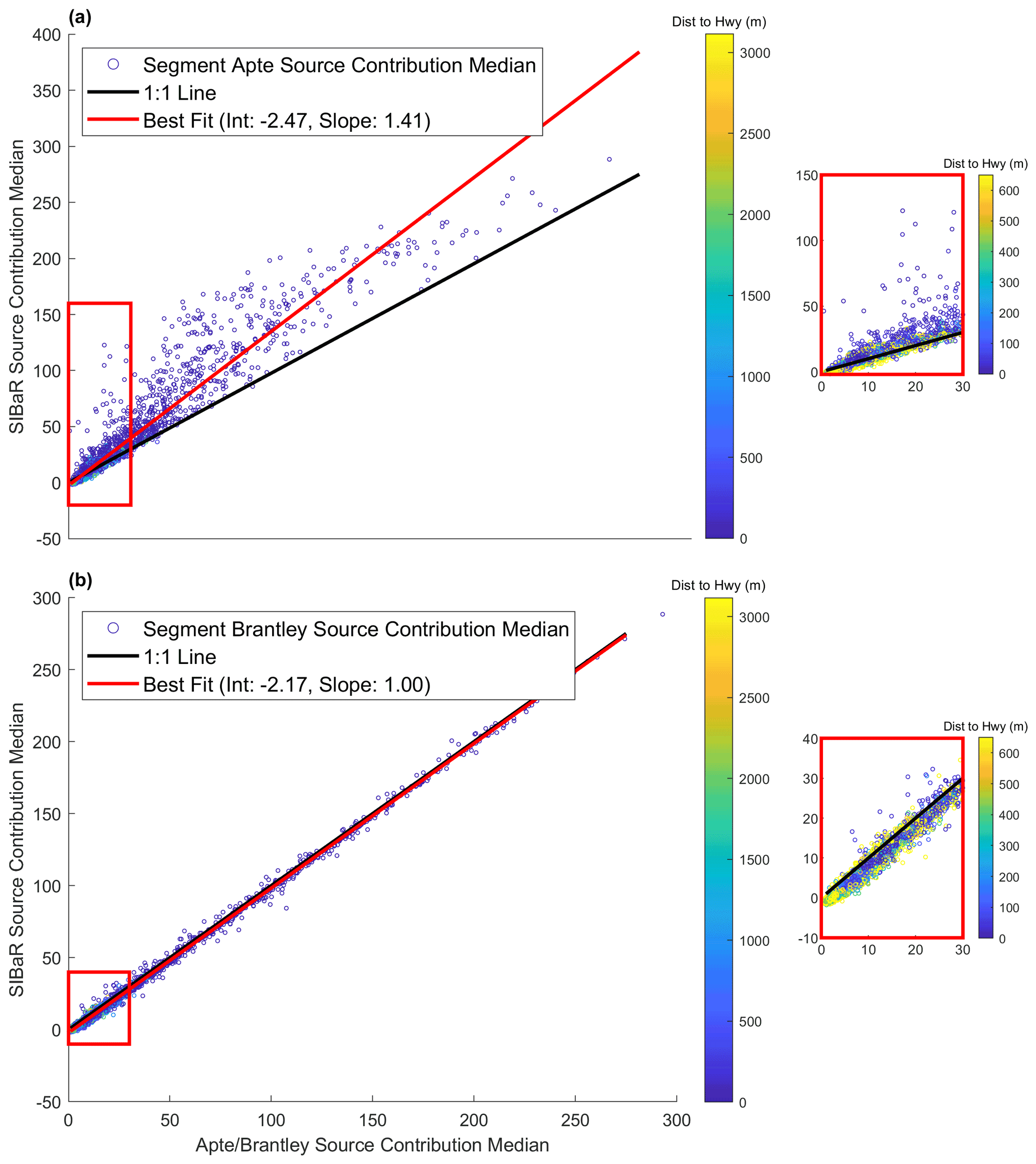
Figure 6Scatterplots of road segment median source contributions predicted by two different techniques against their corresponding SIBaR median source contributions for NOx. The line of best fit is derived using OLS regression and is depicted in red. The 1 : 1 line is depicted in black. Points are colored by their distance to the closest highway. (a) SIBaR source contribution medians plotted against Apte source contribution medians. (b) SIBaR source contribution medians plotted against Brantley source contribution medians. The plots in red rectangles designate a blown-up portion near the origin.
We plot road segment median source contributions derived by Apte and Brantley algorithms against the road segment median concentrations derived by SIBaR and present the results for NOx in Fig. 6. Additionally, we plot lines of best fit derived using ordinary least squares (OLS) regression. Figure 6a illustrates that SIBaR derives higher source contributions medians than the Apte technique, which is largely driven by differences in highway road segment medians. The slope determined using OLS regression suggests that, on average, SIBaR median source contributions are ∼ 41 % higher than Apte median source contributions. Panel (b) of Fig. 6 comparing Brantley and SIBaR road segment medians indicates much closer agreement between the two techniques, with SIBaR estimating source contribution medians at an average offset of 2 ppb lower than Brantley source contribution medians. Data for CO2 source contribution medians are shown in Figs. S16 and S17.
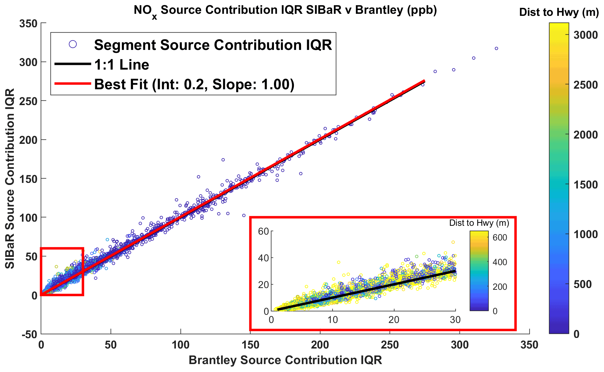
Figure 71 : 1 scatterplot of the interquartile range (IQR) of predicted NOx source contributions at individual road segments for the SIBaR and Brantley techniques. The line of best fit is derived using OLS regression and is depicted in red. The 1 : 1 line is depicted in black. The inset, outlined by the red rectangle, shows the IQR at lower values of the Brantley source contribution IQR. Deviations from the 1 : 1 line suggest that SIBaR captures source influences the Brantley method fails to detect, despite predicting lower source contributions on average and the excellent agreement in median source contribution.
While the road segment median source contributions between the Brantley and SIBaR techniques exhibit strong agreement, we note that source contributions evaluated on a more granular level exhibit some disagreement. Figure 7 displays the inter quartile ranges (IQRs) for source contributions assigned to each road segment plotted against each other for the SIBaR and Brantley techniques, again colored by distance to the closest highway. We display additional 1 : 1 plots of the IQR for different techniques and pollutants (NOx and CO2) in the Supplement (Figs. S18–S20). There are noticeable deviations from the 1 : 1 line in IQR between SIBaR and the Brantley technique for both NOx and CO2, suggesting that the two techniques disagree with one another on individual source contribution drive pass means. Figure S21 displays a histogram of differences in drive pass means between the two techniques. While SIBaR predicts lower source contributions compared to the Brantley technique on average, there are noticeable discrepancies captured in the tails of the distribution.
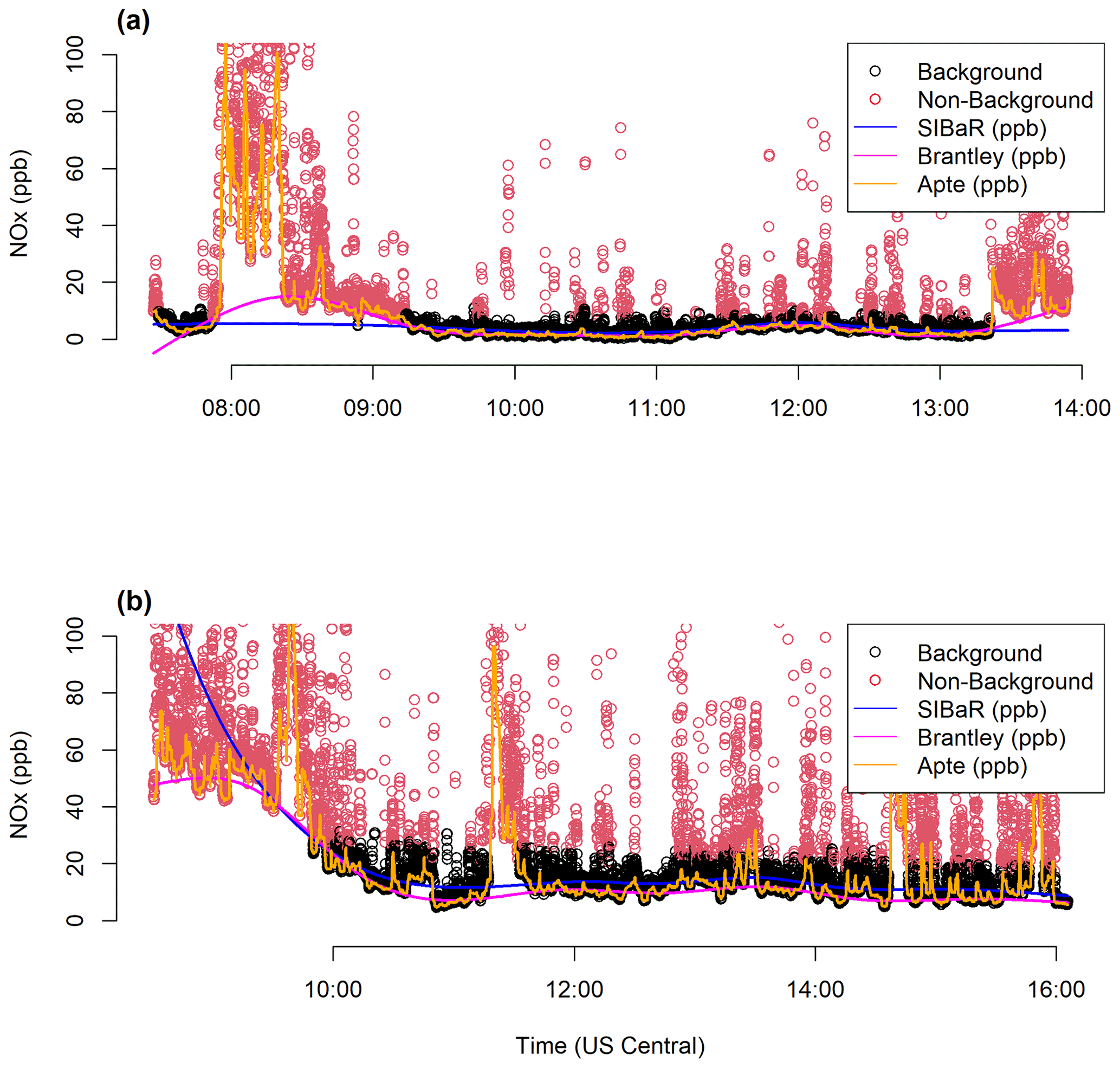
Figure 8Time series plots depicting the original mobile campaign measurements, colored by their SIBaR-decoded states (background and source), along with the background signals generated by the SIBaR, Brantley, and Apte techniques. (a) NOx time series of mobile measurements taken on 3 October 2017, which displays the Apte and Brantley signals overfitting to data decoded as source by the SIBaR partitioning step. (b) NOx time series of mobile measurements taken on 30 November 2017, which shows wildly extrapolated SIBaR predictions at the beginning of the time series due to the lack of background-decoded states.
To provide further context for these results, we present two examples of daily time series of each background technique's predictions in Fig. 8. It is apparent that the Apte technique overfits to the data in both cases. The top panel shows an example of SIBaR's predictions offering an advantage over Brantley's; since SIBaR is fit to a subset of the data, it avoids overfitting in the early morning hours of the time series that the Brantley time series incorporates. Figure 8a illustrates why the cases in the right tail of the histogram in S21 exist. In contrast, the bottom panel showcases the potential faults in using SIBaR predictions; since there are no background designated points at the beginning of this time series example, the spline fit wildly extrapolates, resulting in unrealistic predictions that are captured in the left tail of the histogram in Fig. S21. Both panels illustrate why the medians of Brantley and SIBaR agree so well with one another, yet display IQRs that deviate from their 1 : 1 line. Both signals exhibit strong agreement with one another but can capture different source influences periodically because of the assumptions inherent in each technique. It is also evident that the appropriate background fit would need to be investigated on a case-by-case basis, as one should avoid using the SIBaR technique in instances where extrapolation could occur.
We illustrate that SIBaR provides a defensible mechanism to quantify and remove background from air pollution monitoring data time series. The method's partitioning step is able to match 83 % of a study's previously published background/non-background designations. Mapped distributions of the partitioning step's decoded states show high levels of background state assignment in residential areas, with notable exceptions in hotspots published in a previous study. Finally, we show the impact using SIBaR can have on deriving source contributions in comparing it to the background signals predicted by other techniques. Most notably, SIBaR does not rely on a static time window assumption to determine source impacts, and instead relies on fitting to a subset of the data generated with a time series regime change modeling technique. Setting a static time window can have significant impact on the derived source contributions, as exhibited by the discrepancies between the Apte and SIBaR methods shown in Sect. 3.3. While the SIBaR and Brantley techniques produce similar source contribution medians to one another in the context of this campaign's measurements, both capture different source influences based on the assumptions inherent in each respective technique.
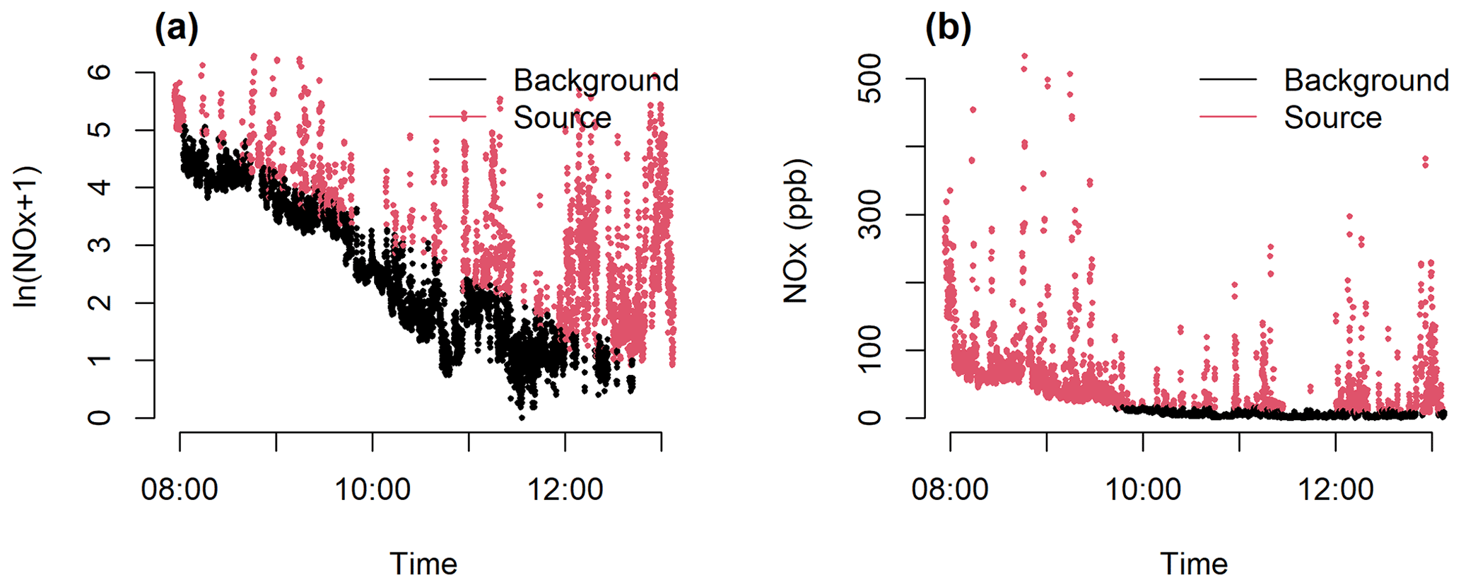
Figure 9Comparison of SIBaR state designations for (a) log-transformed versus (b) non-transformed NOx data on 30 October 2017 (local time, i.e., Central Daylight Time, CDT) in the Houston mobile monitoring campaign. Transformation can affect state assignments, which in this case results in 38 % of the observations having a different categorization upon transformation.
Despite SIBaR's rigor and advancements relative to previously published methods, our approach needs careful consideration and improvement. The method is sensitive to how data in the time series are distributed, and transforming the measurements can provide different results. For example, Fig. 9 exhibits a side-by-side comparison of SIBaR state predictions for transformed (Fig. 9a) and non-transformed (Fig. 9b) NOx data. The transformation in this instance results in portions of the measurements in the early morning period being classified as background, whereas none are designated as background in the non-transformed case. While we think data are more appropriately described in the lognormal regime (Seinfeld and Pandis, 2016), careful consideration of transformation is necessary. Additionally, as discussed in Sect. 3.1 and exhibited in Fig. S4, applying a smoothing time window can also affect the state categorizations.
While the linearity assumption in the time covariate is computationally cheap and easy to implement, it is limited. It is unrealistic to expect background air pollution to exhibit linear behavior, especially as the time series duration extends (Luke et al., 2010). While the linearity assumption seems to be acceptable for time series of several hours of data, problems with that assumption arose in this work and will most likely arise on time series of data by day or when time series are impacted by abrupt meteorological changes. Future work should incorporate assumptions of non-linear behavior into the analysis. Several studies have been published showing the applicability of HMMs to covariates expressed as splines (Langrock et al., 2015, 2018). However, trade-offs between computational time and precision would need to be considered. In its current version, SIBaR takes ∼ 6.5 h to model background for millions of data points (performing the portioning step, evaluating and/or correcting the fit, and fitting the spline for all time series). The Brantley technique, in contrast, takes several minutes.
Despite these shortcomings, SIBaR holds promise as a framework to quantify and remove background from air pollution monitoring time series. In its current state, it is inferior to the Brantley technique with regards to computation time. However, these problems with SIBaR are computational ones rather than problems with its underlying theory. The SIBaR partitioning step captures transient behavior between background and non-background quite well, as the diagnostic results of Sect. 3.1 and the maps in Sect. 3.2 indicate. In addition to addressing other issues highlighted here, future work should focus on methods to reduce its computational time to make its use more straightforward.
Both the code and data are available on request. Additionally, time series comparisons for all 312 time series taken in the campaign, as well as a demo of the SIBaR partitioning step, are available at https://doi.org/10.5281/zenodo.5022590 (Actkinson et al., 2021). Data are also free to download from OpenAQ (https://openaq.org/#/project/28974, Environmental Defense Fund, 2021).
The supplement related to this article is available online at: https://doi.org/10.5194/amt-14-5809-2021-supplement.
BA developed, wrote, and tested the method in R (R: The R Project for Statistical Computing, 2021) with critical input and scientific guidance from RJG and KE. RJG supervised the project and provided feedback on the significance of the method's results. BA wrote the manuscript. All authors contributed to the editing and review of the manuscript.
The authors declare that they have no conflict of interest.
Publisher’s note: Copernicus Publications remains neutral with regard to jurisdictional claims in published maps and institutional affiliations.
We thank Halley Brantley for the provision of data and comments concerning results in Sect. 3.1 of the paper. We also appreciate support from the Environmental Defense Fund for the collection and provision of mobile data.
This research has been supported by the National Institute of Environmental Health Sciences (grant no. R01ES028819-01).
This paper was edited by Glenn Wolfe and reviewed by two anonymous referees.
Actkinson, B., Ensor, K., and Griffin, R. J.: Time Series Comparisons, Model Code, and a Demo Dataset for SIBaR: A New Method for Background Quantification and Removal from Mobile Air Pollution Measurements, Zenodo [data set], https://doi.org/10.5281/zenodo.5022590, 2021.
Apte, J. S., Messier, K. P., Gani, S., Brauer, M., Kirchstetter, T. W., Lunden, M. M., Marshall, J. D., Portier, C. J., Vermeulen, R. C. H., and Hamburg, S. P.: High-Resolution Air Pollution Mapping with Google Street View Cars: Exploiting Big Data, Environ. Sci. Technol., 51, 6999–7008, https://doi.org/10.1021/acs.est.7b00891, 2017.
Baldwin, N., Gilani, O., Raja, S., Batterman, S., Ganguly, R., Hopke, P., Berrocal, V., Robins, T., and Hoogterp, S.: Factors affecting pollutant concentrations in the near-road environment, Atmos. Environ., 115, 223–235, https://doi.org/10.1016/j.atmosenv.2015.05.024, 2015.
Brantley, H. L., Hagler, G. S. W., Kimbrough, E. S., Williams, R. W., Mukerjee, S., and Neas, L. M.: Mobile air monitoring data-processing strategies and effects on spatial air pollution trends, Atmos. Meas. Tech., 7, 2169–2183, https://doi.org/10.5194/amt-7-2169-2014, 2014.
Brantley, H. L., Hagler, G. S. W., Herndon, S. C., Massoli, P., Bergin, M. H., and Russell, A. G.: Characterization of Spatial Air Pollution Patterns Near a Large Railyard Area in Atlanta, Georgia, Int. J. Environ. Res. Public. Health, 16, 535, https://doi.org/10.3390/ijerph16040535, 2019.
Bukowiecki, N., Dommen, J., Prévôt, A. S. H., Richter, R., Weingartner, E., and Baltensperger, U.: A mobile pollutant measurement laboratory – measuring gas phase and aerosol ambient concentrations with high spatial and temporal resolution, Atmos. Environ., 36, 5569–5579, https://doi.org/10.1016/S1352-2310(02)00694-5, 2002.
Caplin, A., Ghandehari, M., Lim, C., Glimcher, P., and Thurston, G.: Advancing environmental exposure assessment science to benefit society, Nat. Commun., 10, 1–11, https://doi.org/10.1038/s41467-019-09155-4, 2019.
Chambliss, S. E., Preble, C. V., Caubel, J. J., Cados, T., Messier, K. P., Alvarez, R. A., LaFranchi, B., Lunden, M., Marshall, J. D., Szpiro, A. A., Kirchstetter, T. W., and Apte, J. S.: Comparison of Mobile and Fixed-Site Black Carbon Measurements for High-Resolution Urban Pollution Mapping, Environ. Sci. Technol., 54, 7848–7857, https://doi.org/10.1021/acs.est.0c01409, 2020.
Chatzis, S. and Varvarigou, T.: A Robust to Outliers Hidden Markov Model with Application in Text-Dependent Speaker Identification, in: 2007 IEEE International Conference on Signal Processing and Communications, 24–27 November 2007, Dubai, United Arab Emirates, 804–807, https://doi.org/10.1109/ICSPC.2007.4728441, 2007.
Chatzis, S. P., Kosmopoulos, D. I., and Varvarigou, T. A.: Robust Sequential Data Modeling Using an Outlier Tolerant Hidden Markov Model, IEEE Trans. Pattern Anal. Mach. Intell., 31, 1657–1669, https://doi.org/10.1109/TPAMI.2008.215, 2009.
Dempster, A. P., Laird, N. M., and Rubin, D. B.: Maximum Likelihood from Incomplete Data Via the EM Algorithm, J. R. Stat. Soc. Ser. B Methodol., 39, 1–22, https://doi.org/10.1111/j.2517-6161.1977.tb01600.x, 1977.
Environmental Defense Fund: Google Earth Outreach, Rice University, and Sonoma Technology: Houston Mobile, OpenAQ [data set], available at: https://openaq.org/#/project/28974, last access: 18 August 2021.
Forney, G. D.: The viterbi algorithm, Proc. IEEE, 61, 268–278, https://doi.org/10.1109/PROC.1973.9030, 1973.
Gómez-Losada, Á., Pires, J. C. M., and Pino-Mejías, R.: Characterization of background air pollution exposure in urban environments using a metric based on Hidden Markov Models, Atmos. Environ., 127, 255–261, https://doi.org/10.1016/j.atmosenv.2015.12.046, 2016.
Gómez-Losada, Á., Pires, J. C. M., and Pino-Mejías, R.: Modelling background air pollution exposure in urban environments: Implications for epidemiological research, Environ. Model. Softw., 106, 13–21, https://doi.org/10.1016/j.envsoft.2018.02.011, 2018.
Gómez-Losada, Á., Santos, F. M., Gibert, K., and Pires, J. C. M.: A data science approach for spatiotemporal modelling of low and resident air pollution in Madrid (Spain): Implications for epidemiological studies, Comput. Environ. Urban Syst., 75, 1–11, https://doi.org/10.1016/j.compenvurbsys.2018.12.005, 2019.
Hankey, S. and Marshall, J. D.: Land Use Regression Models of On-Road Particulate Air Pollution (Particle Number, Black Carbon, PM2.5, Particle Size) Using Mobile Monitoring, Environ. Sci. Technol., 49, 9194–9202, https://doi.org/10.1021/acs.est.5b01209, 2015.
Hankey, S., Sforza, P., and Pierson, M.: Using Mobile Monitoring to Develop Hourly Empirical Models of Particulate Air Pollution in a Rural Appalachian Community, Environ. Sci. Technol., 53, 4305–4315, https://doi.org/10.1021/acs.est.8b05249, 2019.
Hudda, N., Gould, T., Hartin, K., Larson, T. V., and Fruin, S. A.: Emissions from an International Airport Increase Particle Number Concentrations 4-fold at 10 km Downwind, Environ. Sci. Technol., 48, 6628–6635, https://doi.org/10.1021/es5001566, 2014.
Karner, A. A., Eisinger, D. S., and Niemeier, D. A.: Near-Roadway Air Quality: Synthesizing the Findings from Real-World Data, Environ. Sci. Technol., 44, 5334–5344, https://doi.org/10.1021/es100008x, 2010.
Langrock, R., Kneib, T., Sohn, A., and DeRuiter, S. L.: Nonparametric inference in hidden Markov models using P-splines, Biometrics, 71, 520–528, https://doi.org/10.1111/biom.12282, 2015.
Langrock, R., Adam, T., Leos-Barajas, V., Mews, S., Miller, D. L., and Papastamatiou, Y. P.: Spline-based nonparametric inference in general state-switching models, Stat. Neerlandica, 72, 179–200, https://doi.org/10.1111/stan.12133, 2018.
Larson, T., Gould, T., Riley, E. A., Austin, E., Fintzi, J., Sheppard, L., Yost, M., and Simpson, C.: Ambient air quality measurements from a continuously moving mobile platform: Estimation of area-wide, fuel-based, mobile source emission factors using absolute principal component scores, Atmos. Environ., 152, 201–211, https://doi.org/10.1016/j.atmosenv.2016.12.037, 2017.
Li, H. Z., Gu, P., Ye, Q., Zimmerman, N., Robinson, E. S., Subramanian, R., Apte, J. S., Robinson, A. L., and Presto, A. A.: Spatially dense air pollutant sampling: Implications of spatial variability on the representativeness of stationary air pollutant monitors, Atmos. Environ., 2, 100012, https://doi.org/10.1016/j.aeaoa.2019.100012, 2019.
Luke, W. T., Kelley, P., Lefer, B. L., Flynn, J., Rappenglück, B., Leuchner, M., Dibb, J. E., Ziemba, L. D., Anderson, C. H., and Buhr, M.: Measurements of primary trace gases and NOY composition in Houston, Texas, Atmos. Environ., 44, 4068–4080, https://doi.org/10.1016/j.atmosenv.2009.08.014, 2010.
Messier, K. P., Chambliss, S. E., Gani, S., Alvarez, R., Brauer, M., Choi, J. J., Hamburg, S. P., Kerckhoffs, J., LaFranchi, B., Lunden, M. M., Marshall, J. D., Portier, C. J., Roy, A., Szpiro, A. A., Vermeulen, R. C. H., and Apte, J. S.: Mapping Air Pollution with Google Street View Cars: Efficient Approaches with Mobile Monitoring and Land Use Regression, Environ. Sci. Technol., 52, 12563–12572, https://doi.org/10.1021/acs.est.8b03395, 2018.
Miller, D. J., Actkinson, B., Padilla, L., Griffin, R. J., Moore, K., Lewis, P. G. T., Gardner-Frolick, R., Craft, E., Portier, C. J., Hamburg, S. P., and Alvarez, R. A.: Characterizing Elevated Urban Air Pollutant Spatial Patterns with Mobile Monitoring in Houston, Texas, Environ. Sci. Technol., 54, 2133–2142, https://doi.org/10.1021/acs.est.9b05523, 2020.
Patton, A. P., Perkins, J., Zamore, W., Levy, J. I., Brugge, D., and Durant, J. L.: Spatial and temporal differences in traffic-related air pollution in three urban neighborhoods near an interstate highway, Atmos. Environ., 99, 309–321, https://doi.org/10.1016/j.atmosenv.2014.09.072, 2014.
R: The R Project for Statistical Computing, available at: https://www.r-project.org/, last access: 22 June 2021.
Robinson, E. S., Gu, P., Ye, Q., Li, H. Z., Shah, R. U., Apte, J. S., Robinson, A. L., and Presto, A. A.: Restaurant Impacts on Outdoor Air Quality: Elevated Organic Aerosol Mass from Restaurant Cooking with Neighborhood-Scale Plume Extents, Environ. Sci. Technol., 52, 9285–9294, https://doi.org/10.1021/acs.est.8b02654, 2018.
Seinfeld, J. H. and Pandis, S. N.: Atmospheric Chemistry and Physics: From Air Pollution to Climate Change, John Wiley & Sons, Hoboken, New Jersey, USA, 1146 pp., 2016.
Shairsingh, K. K., Jeong, C.-H., Wang, J. M., and Evans, G. J.: Characterizing the spatial variability of local and background concentration signals for air pollution at the neighbourhood scale, Atmos. Environ., 183, 57–68, https://doi.org/10.1016/j.atmosenv.2018.04.010, 2018.
Svensén, M. and Bishop, C. M.: Robust Bayesian mixture modelling, Neurocomputing, 64, 235–252, https://doi.org/10.1016/j.neucom.2004.11.018, 2005.
Tessum, M. W., Larson, T., Gould, T. R., Simpson, C. D., Yost, M. G., and Vedal, S.: Mobile and Fixed-Site Measurements To Identify Spatial Distributions of Traffic-Related Pollution Sources in Los Angeles, Environ. Sci. Technol., 52, 2844–2853, https://doi.org/10.1021/acs.est.7b04889, 2018.
TIGER/Line Shapefile: Harris County, TX, All Roads County-based Shapefile, available at: https://catalog.data.gov/dataset/tiger-line-shapefile-2018-county-harris-county-tx-all-roads-county-based-shapefile (last access: 19 October 2020), 2018.
Van den Bossche, J., Peters, J., Verwaeren, J., Botteldooren, D., Theunis, J., and De Baets, B.: Mobile monitoring for mapping spatial variation in urban air quality: Development and validation of a methodology based on an extensive dataset, Atmos. Environ., 105, 148–161, https://doi.org/10.1016/j.atmosenv.2015.01.017, 2015.
Visser, I. and Speekenbrink, M.: depmixS4: An R Package for Hidden Markov Models, J. Stat. Softw., 36, 1–21, https://doi.org/10.18637/jss.v036.i07, 2010.
Zhang, X., Chen, X., and Zhang, X.: The impact of exposure to air pollution on cognitive performance, Proc. Natl. Acad. Sci. USA, 115, 9193–9197, https://doi.org/10.1073/pnas.1809474115, 2018.