the Creative Commons Attribution 4.0 License.
the Creative Commons Attribution 4.0 License.
 | 27 Aug 2021
Improvement of Odin/SMR water vapour and temperature measurements and validation of the obtained data sets
Francesco Grieco
Kristell Pérot
Donal Murtagh
Patrick Eriksson
Bengt Rydberg
Michael Kiefer
Maya Garcia-Comas
Alyn Lambert
Kaley A. Walker
Its long photochemical lifetime makes H2O a good tracer for mesospheric dynamics. Temperature observations are also critical to study middle atmospheric dynamics. In this study, we present the reprocessing of 18 years of mesospheric H2O and temperature measurements from the Sub-Millimetre Radiometer (SMR) aboard the Odin satellite, resulting in a part of the SMR version 3.0 level 2 data set. The previous version of the data set showed poor accordance with measurements from other instruments, which suggested that the retrieved concentrations and temperature were subject to instrumental artefacts. Different hypotheses have been explored, and the idea of an underestimation of the single-sideband leakage turned out to be the most reasonable one. The value of the lowest transmission achievable has therefore been raised to account for greater sideband leakage, and new retrievals have been performed with the new settings. The retrieved profiles extend between 40–100 km altitude and cover the whole globe to reach 85∘ latitudes. A validation study has been carried out, revealing an overall better accordance with the compared instruments. In particular, relative differences in H2O mixing ratio are always in the ±20 % range between 40 and 70 km and diverge at higher altitudes, while temperature absolute differences are within ±5 K between 40–80 km and also diverge at higher altitudes.
- Article
(18165 KB) - Full-text XML
- BibTeX
- EndNote


With a lifetime of the order of months at the stratopause and of a few days at 100 km, H2O is an important tracer of mesospheric circulation. It is also a main source of hydrogen radicals (such as OH, H, HO2) that are involved in ozone destruction in the middle atmosphere. Methane (CH4) oxidation is a source of H2O in the upper stratosphere, where it is chemically destroyed, primarily through reaction with OH and O(1D), and in the mesosphere, where it is photodissociated by Lyman alpha radiation. Most of the hydrogen from the destroyed CH4 is eventually oxidized to H2O through two reactions (Brasseur and Solomon, 2005):
Another major source of H2O in the stratosphere is the uplift of moist air in the tropical tropopause. Due to vertical transport, this moist air can also reach the mesosphere and affect local H2O abundance. The only major sink of H2O in the mesosphere is photodissociation:
which becomes more important with altitude and dominates over production above 70 km, resulting in a decrease of H2O concentration with increasing altitude. Vertical motions due to the meridional circulation also play a major role. The downwelling during polar winter and the upwelling during polar summer result, respectively, in lower H2O concentrations in the upper stratosphere and mesosphere during polar winters and in larger H2O concentrations during polar summers (Lossow et al., 2019). Moreover, the very cold polar summer mesopause is favourable for the formation of polar mesospheric clouds (e.g. Thomas, 2015; Pérot et al., 2010; Christensen et al., 2016). The deposition of water around 85–90 km to form these clouds leads to a decrease of water vapour at those altitudes. The ice particles grow, sediment, reach the warmer regions at lower altitudes, where they sublimate, leading to an increase of water vapour around 80 km.
Satellite observations of H2O in the middle atmosphere have been performed since the 1970s with the launch of Nimbus-7 satellite and the activity of two instruments on board: LIMS (Limb Infrared Monitor of the Stratosphere) (Remsberg et al., 1984) and SAMS (Stratospheric and Mesospheric Sounder) (Munro and Rodgers, 1994). Currently operational instruments measuring H2O in the middle atmosphere include SABER (Sounding of the Atmosphere using Broadband Emission Radiometry) (Feofilov et al., 2009; Rong et al., 2019) launched aboard TIMED (Thermosphere-Ionosphere-Mesosphere Energetics and Dynamics) in 2001, ACE-FTS (Atmospheric Chemistry Experiment – Fourier Transform Spectrometer) (Nassar et al., 2005) and MAESTRO (Measurement of Aerosol Extinction in the Stratosphere and Troposphere Retrieved by Occultation) (Sioris et al., 2010) launched aboard Scisat-1 in 2003, and MLS (Microwave Limb Sounder) (Waters et al., 2006) launched aboard the Aura satellite in 2004. Moreover, in 2002, three instruments performing middle atmospheric H2O observations were launched aboard the Envisat satellite: GOMOS (Global Ozone Monitoring by Occultation of Stars) (Montoux et al., 2009), MIPAS (Michelson Interferometer for Passive Atmospheric Sounding (e.g. Fischer et al., 2008) and SCIAMACHY (Scanning Imaging Absorption Spectrometer for Atmospheric Chartography) (e.g. Weigel et al., 2016). Their activity stopped in April 2012 due to loss of contact with the satellite.
The Sub-Millimetre Radiometer (SMR) aboard the Odin satellite has been performing H2O measurements in the middle atmosphere since its launch in 2001 and is still operating. Previous studies using SMR H2O observations have been carried out by Lossow et al. (2007, 2008, 2009) and Urban et al. (2007). These studies refer to SMR v2.1 L2 data retrieved from the 556.9 GHz H2O line. In the mesosphere, these profiles are biased high compared to other instruments, i.e. around 20 % between 40–70 km and by more than 50 % between 70–100 km (Murtagh et al., 2020).
Together with H2O, temperature is also a retrieval product obtained from the same spectra and it represents another useful tool to study the middle atmospheric dynamics. Moreover, increasing concentrations of greenhouse gases are expected to lead to cooling of the mesosphere, increasing interest in studies of long-term temperature trends in the middle atmosphere. The SMR v2.1 temperature retrieved together with H2O shows biases up to 15 K in the mesosphere (Murtagh et al., 2020). One of the first studies of this kind based on satellite observations was carried out using data from SME (Solar Mesosphere Explorer) (Clancy and Rusch, 1989). Apart from SMR, in recent years, other satellite instruments have been employed for temperature measurements of this atmospheric region. Among these there are MLS (Azeem et al., 2001) and HALOE (Halogen Occultation Experiment) (Hervig et al., 1996) launched in 1991 aboard UARS (Upper Atmosphere Research Satellite), TIMED/SABER (Dawkins et al., 2018), Envisat/MIPAS (Kiefer et al., 2021), Aura/MLS (Schwartz et al., 2008), Scisat-1/ACE-FTS (Sica et al., 2008) and SOFIE (Solar Occultation for Ice) (Stevens et al., 2012) launched in 2007 aboard the AIM (Aeronomy of Ice in the Mesosphere) satellite.
The Odin/SMR data set has undergone a full reprocessing, leading to a new version (v3.0). The present study, carried out to identify the instrumental origins of the above-mentioned biases, is part of this extensive reprocessing work. The improved retrieval method will be described in Sect. 2.1. The resulting H2O and temperature data sets are presented in Sect. 3 and validated in Sect. 4 by comparing them with independent satellite measurements from MIPAS, ACE-FTS and MLS. These instruments and Odin/SMR are introduced in the next section.
2.1 Odin/SMR
2.1.1 The sub-millimetre radiometer
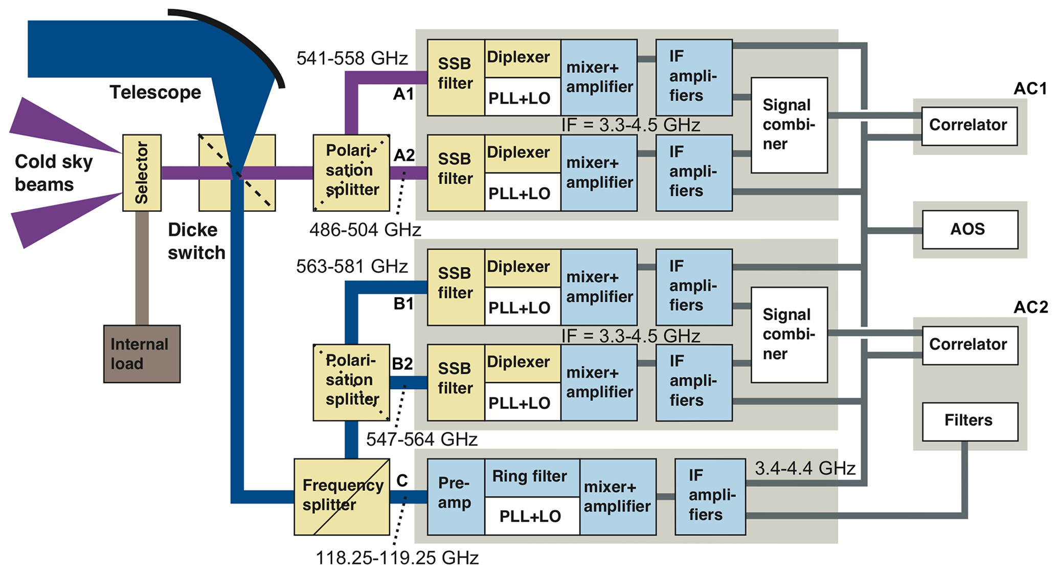
The Sub-Millimeter Radiometer (SMR) is an instrument aboard the Odin satellite performing limb sounding of the middle atmosphere. The measurements cover the whole globe including the polar regions. Odin was launched on 20 February 2001 as a Swedish-led project in collaboration with Canada, France and Finland. Its 600 km Sun-synchronous orbit has an inclination of 97.77∘ and a 18:00 LT ascending node (slightly varying with time). SMR has four sub-millimetre receivers: one covering frequencies between 486–504 GHz and three others overlapping to cover 541–581 GHz, as well as a millimetre receiver measuring radiation around 118 GHz, so that emissions from O3, H2O, CO, NO, ClO, N2O, HNO3 and O2 due to rotational transitions can be detected (Frisk et al., 2003). SMR components are schematized in Fig. 1. A Dicke switch rapidly changes the source of input radiation between the main beam and calibrators (cold sky and hot load); the radiation is then split according to polarization and collected by different receivers; here, it is combined with a local oscillator (LO) signal by means of a mixer, converting the signal to lower frequencies (3.3–4.5 GHz) and maintaining only the contribution from two sidebands. SMR is a single-sideband instrument; it uses a Martin–Puplett interferometer with arm lengths tuned to optimize transmission of the primary band (containing the signals of scientific interest) while suppressing transmission of the other (image) sideband. The response of the interferometer with regards to frequency ν is equal to
where l is the interferometer length, and r0 is the lowest transmission value achieved (Eriksson and Urban, 2006); r0 is not zero because it is not possible to achieve perfect suppression. The linear dependency of l with respect to the temperature aboard the satellite is also taken into account:
where T is the temperature of the satellite, l0 is the interferometer length at the reference temperature T0, lsb is the nominal sideband path tuning length (expressed for both arms altogether, hence the division by 2), and cT is the coefficient of thermal expansion. Values of l0, T0 and cT have been estimated by Eriksson and Urban (2006) from fits based on various observations. Since it is impossible to completely suppress the image band contribution, a sideband leakage (p) is included in the measurement, where p is defined as
with ν and ν′ being, respectively, the primary band and image band centre frequencies. Eventually, the signal is amplified and directed to the spectrometers.
The observation time of the instrument was equally shared between astronomical and atmospheric observations until 2007, and subsequently the instrument has been exclusively employed to perform atmospheric measurements. SMR measures spectra during upward and downward vertical scanning of the atmospheric limb from the upper troposphere to the lower thermosphere. However, in this study, we consider only mesospheric measurements ranging from 40 to 100 km.
2.1.2 SMR H2O and temperature measurements: description and improvement
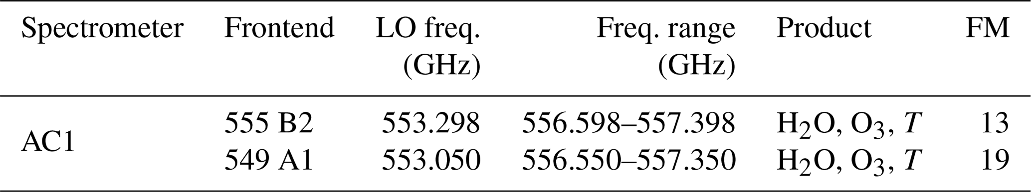
SMR receivers can be set up to cover different frequency bands. Each of these configurations, called frequency modes (FMs), are assigned scheduled observation times. In this study, we focus on mesospheric observations of the 556.9 GHz emission line from the corresponding H2O rotational transition. They are performed with a 3–4 km vertical resolution, using FM13 and FM19 (while stratospheric observations are performed using other FMs) whose characteristics are summarized in Table 1. With these FMs, temperature and O3 are retrieved, although the latter is not the focus of this paper. The retrieval of temperature is made possible by the fact that the 556.9 GHz H2O emission line is saturated up to around 90 km (Murtagh et al., 2020).
Table 1Characteristics of the FMs used to observe mesospheric H2O and temperature from Rydberg et al. (2017).
The two FMs use different frontends, that is the set of components denoted by B2 and A1 in Fig. 1. The retrievals were carried out using the Atmospheric Radiative Transfer Simulator (ARTS), which is a software package for long wavelength radiative transfer simulations, with a focus on passive microwave observations, incorporating effects of sensor characteristics (e.g. Eriksson et al., 2011). ARTS retrieval algorithms are based on the optimal estimation method (e.g. Rodgers, 2000). In this study, a mesospheric inversion mode was used, performing retrievals from measurements with tangent altitudes between 40 and 100 km. A more detailed description of the retrieval process for v3.0 can be found in Grieco et al. (2020). The temperature a priori up to 60 km is provided by ERA-Interim reanalysis data (Dee et al., 2011), and above 70 km the Mass Spectrometer Incoherent Scatter model (version NRLMSISE-00; Picone et al., 2002) is used. Between 60–70 km, a spline interpolation of the two is applied. The a priori for water vapour is a compilation from the Bordeaux Observatory. Both temperature and water vapour a priori are made available together with the retrieved profiles.
In SMR v2.1, H2O profiles retrieved from FM13 and FM19 differ significantly from measurements of other satellites. FM19 has a bias between ±20 % between 40 and 80 km, while FM13 has concentrations around 10 % higher than Scisat-1/ACE-FTS and Aura/MLS between 40 and 60 km, and around 20 % higher than Envisat/MIPAS in the same altitude range. Both FMs showed differences greater than −50 % between 80 and 100 km. Temperature bias for FM19 is about −5 to −10 K between 60 and 80 km and, for FM13, the bias is equal to about +10 K between 40 and 80 km. Both FMs were characterized by very high negative biases at high altitudes. These differences can be seen in Figs. 12 and 13, as well as in Murtagh et al. (2020), who used a smaller data set for comparison. This suggested the presence of instrumental artefacts. We investigated for possible nonlinearity in the spectra and for erroneous estimations of the pointing offset of the instrument; however, an underestimation of r0 (see Eq. 1) turned out to be the most likely cause of the incongruous retrieved quantities. Sideband leakages greater than the nominal value have been already observed in spectra in Eriksson and Urban (2006). A r0 of −14 dB had previously been assumed for both frontends used in the two FMs under consideration: an underestimation that caused spurious signal originated from the sideband leakage to be considered as part of the signal of interest, leading to misestimation of retrieved mixing ratio and temperature. Setting the r0 value to −13 dB for FM13 and to −11 dB for FM19 gave the best empirical results in terms of minimizing the differences with measurements from other instruments (see Sect. 4).
H2O retrieval for a nominal scan is shown in Fig. 2. A measure of how much a retrieved quantity is influenced by the a priori is given by the measurement response, a quantity defined as the sum over the row of the averaging kernel matrix (Rodgers, 2000). Data with a measurement response lower than 0.75 are discarded. This is the case for the retrieved profile above 100 km which is, nevertheless, shown here out of completeness as well as high altitudes averaging kernels.
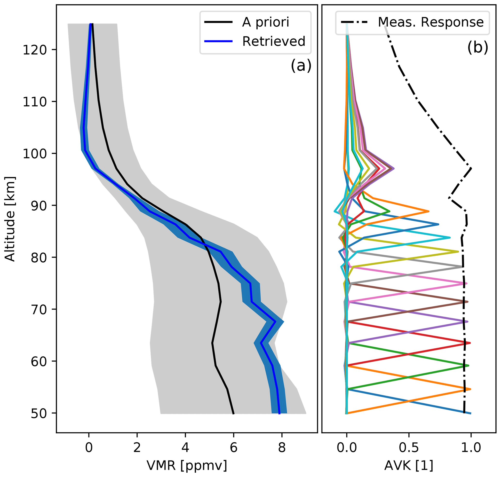
Figure 2Example retrieval from ScanID 230753751 from FM19. (a) Retrieved mixing ratio profile and error due measurement thermal noise (Rodgers, 2000) (in blue and shaded, respectively) and a priori including uncertainties (in black and shaded, respectively). (b) Averaging kernels plotted in a different colour for each altitude (not indicated) and measurement response (dashed–dotted black line).
2.2 Validation data sets
2.2.1 MIPAS
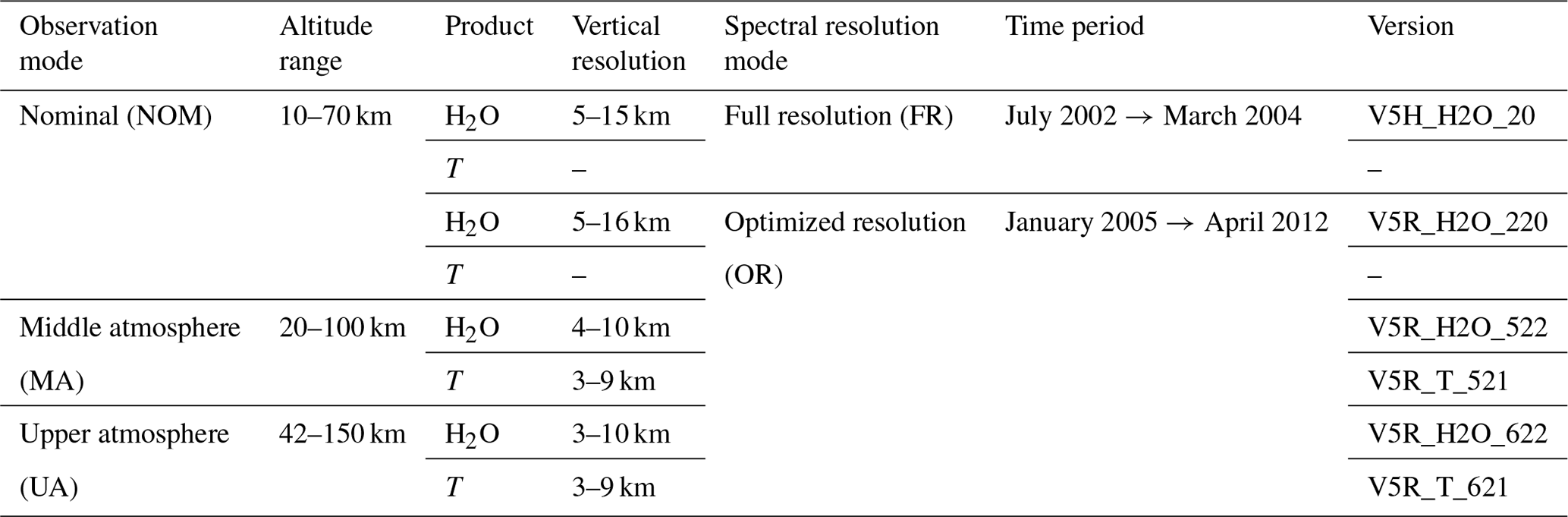
The Michelson Interferometer for Passive Atmospheric Sounding (MIPAS) aboard Envisat performed mid-infrared limb sounding of the atmosphere from June 2002 until April 2012, when contact with the satellite was lost. Envisat was on a 98.55∘ inclination and 22:00 LT ascending node Sun-synchronous orbit at 800 km altitude. The retrieval products used for comparison in this study are obtained with the retrieval processor developed at the Karlsruhe Institute of Meteorology and Climate Research (IMK) and the Instituto de Astrofisica de Andalucia (IAA) (von Clarmann et al., 2009). The MIPAS V5 data sets used for validation are those from the nominal (NOM), middle atmosphere (MA) and upper atmosphere (UA) observation modes, whose characteristics are summarized in Table 2. The forward model used for MA and UA modes includes non-LTE effects (Funke et al., 2001). Quality filtering of the data, as indicated in Kiefer and Lossow (2017), has been performed. In March 2004, MIPAS malfunctioned and did not return to operation until January 2005. During the first period, the instrument was being used in full spectral resolution (FR mission), while, in the second period, it operated with a reduced spectral resolution (OR mission) (Oelhaf, 2008).
Table 2Characteristics of the MIPAS H2O and temperature data sets used for comparison. Vertical resolutions refer to the observations in the altitude range 40–100 km considered in this study.
2.2.2 ACE-FTS
The Fourier Transform Spectrometer (FTS), an instrument which is part of the Canadian-led Atmospheric Chemistry Experiment (ACE), was launched aboard Scisat-1 on 12 August 2003 and is still operational. Scisat-1 is in a 650 km orbit with a 74∘ inclination. ACE-FTS is a solar occultation instrument that measures H2O mixing ratio between 5 and 100 km, and temperature to 125 km, with a 3–4 km vertical resolution. In this work, we use the ACE-FTS v3.6 data set (Sheese et al., 2017), quality filtered as indicated by the instrument team (Sheese et al., 2015).
2.2.3 MLS
The MLS on the Aura satellite has operated nearly continuously since 15 July 2004, on a 705 km Sun-synchronous orbit characterized by a 98∘ inclination and a 13:45 LT ascending node. We use MLS v5 data sets of temperature (measured between 261–0.00046 hPa) and H2O mixing ratio (measured between 316–0.001 hPa), characterized respectively by 7–12 and 3–6 km vertical resolutions, to which the recommended quality filtering has been applied (Livesey et al., 2020).
In this section, we present the SMR v3.0 L2 H2O and temperature products retrieved from FM13 and FM19 measurements, produced using the improved retrieval algorithms described in the previous section. In particular, we describe H2O mixing ratio and temperature time series and compare the retrieved profiles to the previous v2.1 data set.

Figure 3Number of L1 and L2 scans by month for FM13 (a) and FM19 (b). The ticks on the x axis correspond to 1 January for each year.
Figure 3 shows a histogram summarizing the number of L1 and L2 products available for FM13 and FM19 during the whole Odin operational time period. The amount of L2 data is generally lower than L1 data since the retrieval process does not succeed for every scan. Since 2006, the two FMs have been used in similar proportion, but in the earlier years, FM13 was used only occasionally, with a particularly high number of measurements performed during July 2002, July 2003 and August 2004. These are associated with a special scheduling set to study dynamics in the northern summer mesosphere related to the presence of noctilucent clouds (Karlsson et al., 2004).
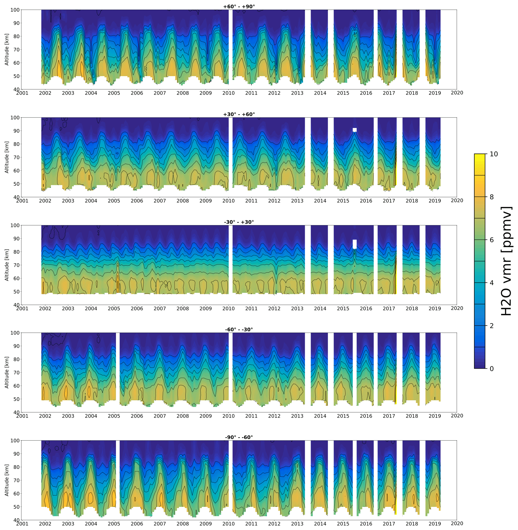
Figure 4Time series of FM19 H2O volume mixing ratios measured by SMR for different latitude bands. The white areas indicate periods and altitudes at which the number of measurements in the given latitude band is lower than 10. The ticks on the x axis correspond to the beginning of each year.

Figure 5Time series of FM19 temperature measured by SMR for different latitude bands. The white areas indicate periods and altitudes at which the number of measurements in the given latitude band is lower than 10. The ticks on the x axis correspond to the beginning of each year.
Figures 4 and A1 show time series of H2O volume mixing ratios corresponding to FM13 and FM19, respectively, in the form of monthly zonal means over five latitude bands covering the whole globe. The equivalent figures for retrieved temperature are shown in Figs. 5 and A2. The gaps in the data sets observed globally every northern summer from 2013 result from the ageing instrument being put in standby mode during the eclipse season in order to save battery power. In the tropics, we observe a clear semi-annual oscillation (SAO) pattern above 75 km, in both the H2O and temperature data sets. This phenomenon is caused by SAO of the zonal winds in the mesosphere which is driven by momentum deposition from gravity and Kelvin waves coming from lower altitudes. Zonal wind SAOs in turn give rise to SAO in meridional and vertical advection (Hamilton, 2015). In particular, descent or weakened ascent near the equinoxes results in lower H2O concentrations in the mesosphere in the tropics, while stronger ascent during solstices results in higher H2O concentrations (e.g. Lossow et al., 2017). High latitudes are dominated by an annual cycle that features, at all altitudes and for both hemispheres, higher concentrations during local summertime, caused by upward transportation of moist air and increased methane oxidation due to the greater amount of received solar radiation, and lower concentrations during local wintertime, due to the descent of dry air from the upper mesosphere via the downward branch of the mesospheric residual circulation. The amplitude of this oscillation is bigger in the Southern Hemisphere, where the descent of air is stronger and more stable (Lossow et al., 2017). Summer temperature minima in the upper mesosphere result from gravity wave forcing that pushes this high-altitude region away from geostrophic balance, leading to the mesospheric residual circulation. This circulation pattern is associated with upward motion of air during summertime that results in a strong adiabatic cooling (Brasseur and Solomon, 2005). Moreover, in the northern high latitudes, some particular features are observed in some years (namely 2004, 2006, 2009, 2013 and 2019) during late winter. Each is due to a sudden stratospheric warming (SSW) followed by the formation of an elevated stratopause (Vignon and Mitchell, 2015). Secondary maxima in H2O mixing ratio correspond to the onset of the SSW events during which the polar vortex was disturbed by planetary waves (e.g. Charlton and Polvani, 2007). Following these SSWs, the polar vortex recovered and the stratopause reformed at higher altitudes than normal, corresponding to the peaks in temperature observed around 80 km in Figs. 5 and A2. Such events are associated with increased downward motion of air in the mesosphere (e.g. Pérot et al., 2014). This leads to transport of dry air from the upper mesosphere down to the lower mesosphere, as seen in Figs. 4 and A1. Midlatitudes show, in a less pronounced way, both effects of SAO and annual cycle. Finally, at all latitudes, lower H2O concentrations can be observed at high altitudes during the period 2012–2016 due to increased photolysis related to a stronger solar activity. On the other hand, at low altitudes, higher H2O concentrations can be observed due to increased O2 photolysis and consequent enhanced CH4 oxidation (e.g. Remsberg et al., 2018).
In Figs. A3 and A4, we compare the data sets corresponding to the two frequency modes considered in the study, for H2O and temperature, respectively. As explained in Sect. 2.1.2, those correspond to measurements made using different parts of the instrument. They should therefore be treated as two different data sets. Here, non-coincident profiles are compared, since the temporal and geographical coverage is different for the two frequency modes. Differences are therefore to be expected. These comparisons are simply shown with the aim of summarizing the average differences between the FMs, which could be useful information for the future users of these data sets. In Fig. A3, the v3.0 FM13–FM19 H2O relative difference is shown. It is equal to −15 % at 40 km altitude; the value then reaches 0 % at 50 km and remains approximately constant until 60 km. It then increases to reach +100 % at 85 km altitude and finally decreases back to 0 % at 100 km altitude. The high relative difference values around 85 km are observed at all latitudes and seasons (not shown). Moreover, the v3.0 FM13–FM19 absolute difference with regards to temperature (Fig. A4) oscillates between ±8 K and only reaches −16 K around 100 km. The relative difference values are referred to the mean between the FM13 and FM19 products.
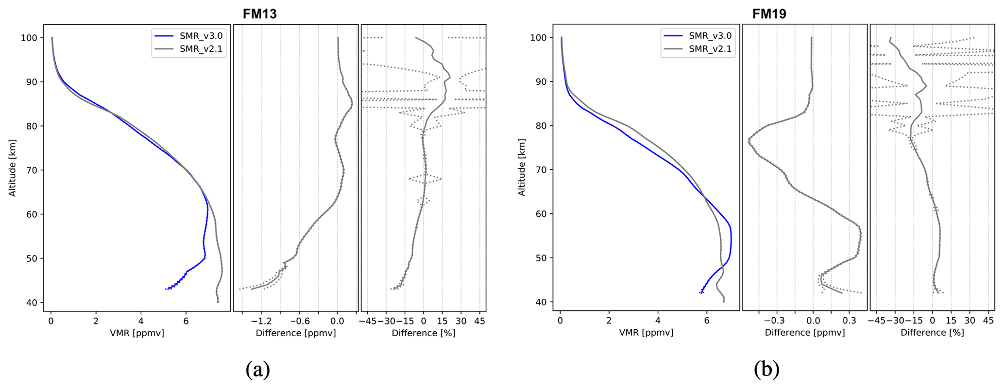
Figure 6Comparison of SMR v3.0 with respect to v2.1 H2O profiles, from FM13 (a) and FM19 (b). The data plotted are global averages over the time period between February 2001 and April 2019. Each subfigure consists of three panels. Left panels show volume mixing ratios, expressed in ppmv. Centre panels show absolute differences, expressed in ppmv. Right panels show relative differences, expressed in percentage. The differences shown are calculated as medians of the single profiles' differences. The dashed lines represent the standard deviation of the median which, in some cases, is smaller than the thickness of the profile line, causing the dashed line not to be distinguishable.
Comparison of SMR v3.0 with respect to the older SMR v2.1 H2O data set (e.g. Urban et al., 2007) shows, for FM13, a relative difference of −25 % around 40 km which goes down to 0 % at 60 km. This corrects for the v2.1 FM13 bias discussed with respect to ACE and MLS (see Sect. 2.1.2). The value stays around 0 % until 80 km and then increases up to +20 % at 90 km, to finally decrease to −7 % at 100 km (Fig. 6a). The v3.0 FM13 higher concentrations above 80 km result in a decrease of the high negative bias that characterized v2.1, although differences with respect to other instruments remain high at these altitudes, as discussed in Sect. 4. Zonal mean plots of difference values averaged over the whole SMR operating time period, for different latitudes and seasons, are shown in the Appendix. Peaks of +30 % are registered during northern spring and summer, as well as during southern summer and during local autumn in both hemispheres, at high latitudes between 80–100 km. Moreover, the highest negative values, of −60 %, are observed during local autumn in both hemispheres, in an area within the tropics and the autumn pole between 90–100 km (Fig. A5). Comparison of FM19 H2O retrievals shows instead a relative difference of 0 % between 40–45 km and of +5 % between 50–60 km. The observed v2.1 FM19 negative bias below 60 km is therefore partly reduced. Then the difference goes down to −15 % at 80 km, back up to −5 % between 85–90 km and then down again to −30 % at 100 km (Fig. 6b). Peaks of −40 % are observed during northern spring and summer at high latitudes around 100 km altitude (Fig. A6). Note that each relative difference value is referred to the mean between the v3.0 and v2.1 concentrations. Temperature profile comparisons, and the zonal means showing differences for the various latitude and seasons, are described below and shown in the Appendix. The retrieved temperature for FM13 is generally lower for v3.0 compared to v2.1, with an absolute difference oscillating between −2.5 and −5 K in the 40–90 km altitude range (Fig. A7a). FM19 v3.0 temperature is instead generally higher than measured in v2.1, with the absolute difference being equal to +7 K at 40 km and then oscillating between +2.5 and +5 K in the 45–90 km altitude range (Fig. A7b). For both frequency modes, the relative differences are very low. These differences show that the data set has been improved, since the previous version was affected by a high bias in the case of FM13 and by a generally low bias in the case of FM19, as described in Sect. 2.1.2. These improvements will be evaluated further in the next section, where the v3.0 data sets will be compared to other instruments.
To evaluate the quality of the new FM13 and FM19 data, in this section, we compare the SMR v3.0 H2O and temperature retrievals from these FMs with nearly coincident measurements from other limb-sounding satellite-borne instruments, such as MIPAS, ACE-FTS and MLS. These instruments have been introduced in Sect. 2.2.
H2O measurements are considered coincident if they occur within a maximum temporal separation of 9 h and maximum spatial separation of 800 km, while for temperature the criteria are 4 h and 1000 km. Performing tests with stricter time coincidence criteria proved not to sensibly change the shape of the median difference profiles. The different criteria depend on the temporal variability of the products and on the amount of data available from the comparison instruments. While ACE-FTS and MLS profiles have similar vertical resolutions to SMR, MIPAS profiles are characterized by more coarse resolutions. Therefore, for comparison with MIPAS, SMR profiles have been smoothed with a Gaussian filter characterized by a full width at half maximum (FWHM) equal to the MIPAS–SMR difference in vertical resolution. Subsequent comparisons are made by interpolating the profiles to a common 40–100 km altitude grid with a 1 km resolution. Denoting with i a pair of coincident measurements, the absolute and relative difference between these profiles are defined, respectively, as
where xSMR and xcomp are the retrieved H2O mixing ratios or temperature at altitude z for the coincidence i, from SMR and the instrument considered for the comparison, respectively. Measurements done by satellite instruments are in general affected by large uncertainties so, when comparing them, their relative difference is with respect to the mean of the two, to avoid preferring either instrument as a reference (Randall et al., 2003). N(z) is the number of differences (absolute or relative) measured at altitude z. Δ(z) is their median. The dispersion of the measurements is represented by the standard deviation of the median:
The median is used, instead of the mean, to minimize the impact of outliers. Below, we present the results of the comparisons in form of profiles averaged over the totality of the coincidences, regardless of time or location. Both H2O and temperature profiles are discussed below, the latter being shown in the Appendix. For the sake of clarity, no monthly or seasonal average profiles are shown, but seasonal zonal means of H2O volume mixing ratio (VMR) relative differences and temperature absolute differences are also included in the Appendix and discussed.
4.1 MIPAS
4.1.1 Nominal mode
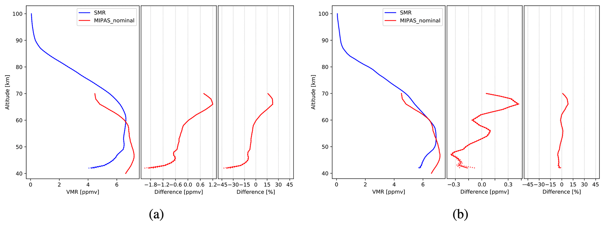
Both MIPAS nominal mode data sets (from FR and OR periods) are here considered for comparison with SMR. Differences between the two reference data sets (FR and OR) are so small in most regions that they do not spoil the comparison, and only between 45–50 km they reach 10 % (not shown). Therefore, the OR and FR data are considered as one data set and comparisons are not presented separately for each of them. In particular, for comparisons with SMR FM13, no variations between FR and OR are to be reported since only a small quantity of SMR FM13 measurements were performed during the period of MIPAS FR mission (see Fig. 3). SMR H2O average profiles for FM13 and FM19, averaged over all the coincidences found, show different agreement with MIPAS. FM19 relative difference (see Fig. 7b) is small between 40 and 60 km altitude staying close to 0 %. Then the difference increases to reach +10 % at 65 km and decreases back to 0 % at 70 km. Looking at latitudes and seasons specifically (Fig. A11), peaks of +20 % are observed around 65 km at high latitudes during local summer and northern spring, while relative differences of −30 % are observed at 70 km during local winter at midlatitudes. FM13 instead (Fig. 7a) presents a major negative difference of −40 % at 40 km, decreasing to −10 % at 45 km. Between 45 and 70 km, the difference value increase and reaches +20 %. The highest positive differences, of +40 % are registered between 60 and 70 km during local summer in both hemispheres and during northern spring (Fig. A10) at high latitudes. Lossow et al. (2019) compared MIPAS H2O with that from correlative measurements and found that, at around 65 km, MIPAS nominal H2O mixing ratio reaches a negative bias of up to −25 %. This might explain the SMR–MIPAS relative differences which we observe around that altitude for both FMs.
4.1.2 Middle atmosphere mode
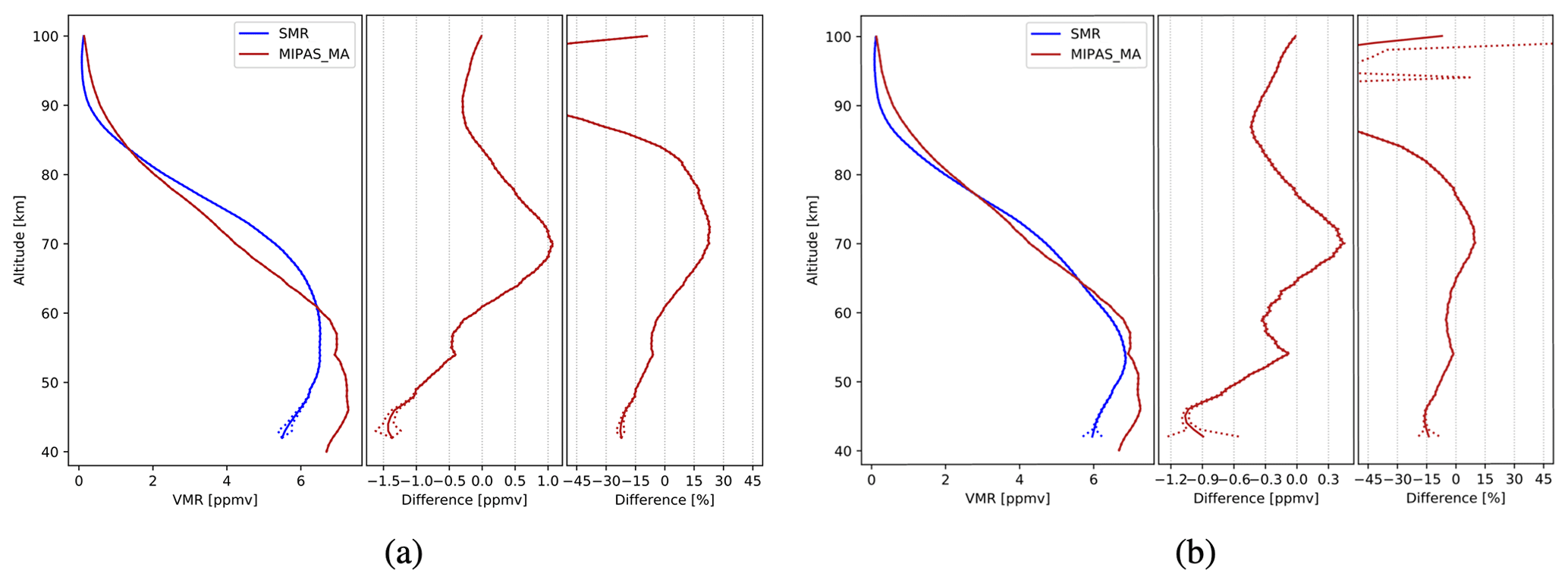
H2O profile comparison between MIPAS OR Middle Atmosphere mode and SMR FM19 shows a relative difference of −15 % at 40 km that increases with altitude to reach 0 % at 55 km and stays roughly constant until 65 km (Fig. 8b). It then increases to +10 % (0.4 ppmv) at 70 km and decreases up to −80 % (out of shown scale; corresponding to −0.4 ppmv) at 90 km; finally, it increases again to reach −5 % at 100 km. For FM13 (Fig. 8a), the relative difference has a value of −20 % at 40 km and increases to 0 % at 60 km. It increases up to around 20 % (corresponding to 1 ppmv absolute difference) at 70 km and then it decreases to −100 % (−0.3 ppmv) around 90 km and goes up again to around −10 % at 100 km. The SMR–MIPAS differences observed for both FMs between 40 and 60 km are consistent with the MIPAS MA high bias reported by Lossow et al. (2019) at those altitudes. For both FMs, peaks of −150 % are observed for all seasons between 90 and 100 km at low latitudes. At the same altitudes, smaller differences during polar winter are observed. This is probably explained by non-LTE effects being less important there (Figs. A12 and A13). Note that very high values in H2O relative difference are to be expected at high altitudes due to the extremely low concentrations in that region. Temperature absolute differences are close to 0 K between 40 and 80 km and decrease down to −45 K at higher altitudes, for both FMs (Fig. A20).
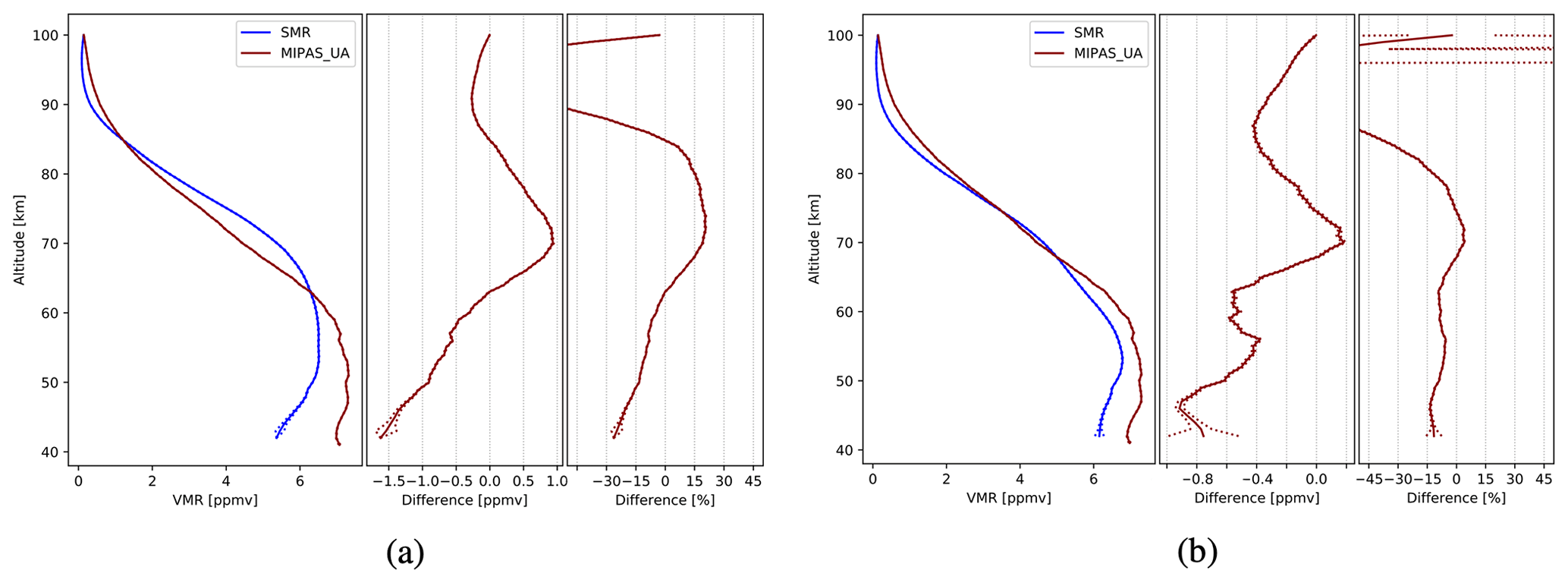
4.1.3 Upper atmosphere mode
H2O average relative differences between SMR and MIPAS OR upper atmosphere profiles present a value of −30 % at 40 km for FM13 (Fig. 9a) which gets smaller with altitude to reach 0 % at 60 km. The value keeps increasing with altitude until 70 km where it reaches +20 % (1 ppmv), it stays roughly constant until 80 km, decreases to about −100 % (−0.3 ppmv) at 90 km and finally increases back to 0 % at 100 km. Relative difference regarding FM19 (Fig. 9b) is equal to −15 % at 40 km; it oscillates between −10 % and −5 % until 65 km and reaches 0 % at 70 km; it then decreases to reach −100 % (−0.4 ppmv) at 90 km and increases back to 0 % at 100 km. Peaks of −150 % are registered between 90 and 100 km at low latitudes during all seasons for both FMs (Figs. A14 and A15), as well as a peak of +90 % during southern winter at high latitudes. Temperature absolute difference is similar to what was observed in the comparison with the middle atmosphere mode (Fig. A23).
4.2 ACE-FTS
SMR–ACE H2O profile comparison, using FM13 (Fig. 10a), shows a −70 % relative difference at 40 km, then the value goes steeply to 0 % and stays almost constant between 45 and 80 km altitude. Between 80 and 100 km, the relative difference value goes down and reaches values of −140 % (corresponding to absolute differences in the order of −0.01 ppmv). For FM19 (Fig. 10b), the measured relative difference is −15 % below 45 km and reaches 0 % at 50 km; it then decreases slowly with altitude until 80 km, where it is equal to −30 % (−0.40 ppmv absolute difference). Between 80 and 100 km, it decreases more rapidly to about −60 % (corresponding to an absolute difference in the order of −0.01 ppmv). Regarding temperature (Fig. A26), FM13 absolute difference stays between 0 and 4 K until 80 km altitude, and at higher altitudes it oscillates between lower values within 0 and −16 K. For FM19 instead, it assumes values between 0 and 7 K until 50 km, then it slowly decreases up to −15 K at 90 km, and between 90 and 100 km the difference is characterized by considerably lower values with a minimum of −60 K.

4.3 MLS
Comparing SMR H2O profiles from FM13 with MLS (Fig. 11a), we observe a relative difference of −30 % at 40 km which rapidly goes up to 0 % at 45 km and then remains constant until 65 km altitude. The value then decreases to reach −30 % (−0.6 ppmv absolute difference) at 80 km. Above 80 km, it decreases rapidly with altitude and reaches −140 % (-2 ppmv) at 95 km. Regarding comparison with FM19 profiles, the difference is equal to 0 % between 40 and 60 km. Between 60 and 80 km, it goes down to −30 % (−1 ppmv) and then quickly decreases with altitude down to −165 % (−1.25 ppmv) at 95 km. Peaks of −150 % are observed at 90 km during local winter and autumn in both hemispheres for both FMs (Figs. A18 and A19). Temperature absolute difference for FM13 (Fig. A29a) is equal to 8 K at 40 km, goes to 0 K at 45 km and increases back up to 8 K at 60 km. The value is constant with altitude between 60–70 km. The difference then decreases down to −2 K around 90 km, goes back to 8 K at 95 km and decreases to −3 K at 100 km. FM19 shows a decrease in temperature from 10 K at 40 km to 5 K at 45 km (Fig. A29b). The value stays constant between 45 and 55 km and then decreases with altitude to reach −5 K around 90 km. Finally, an absolute difference of 0 K is reached around 100 km.
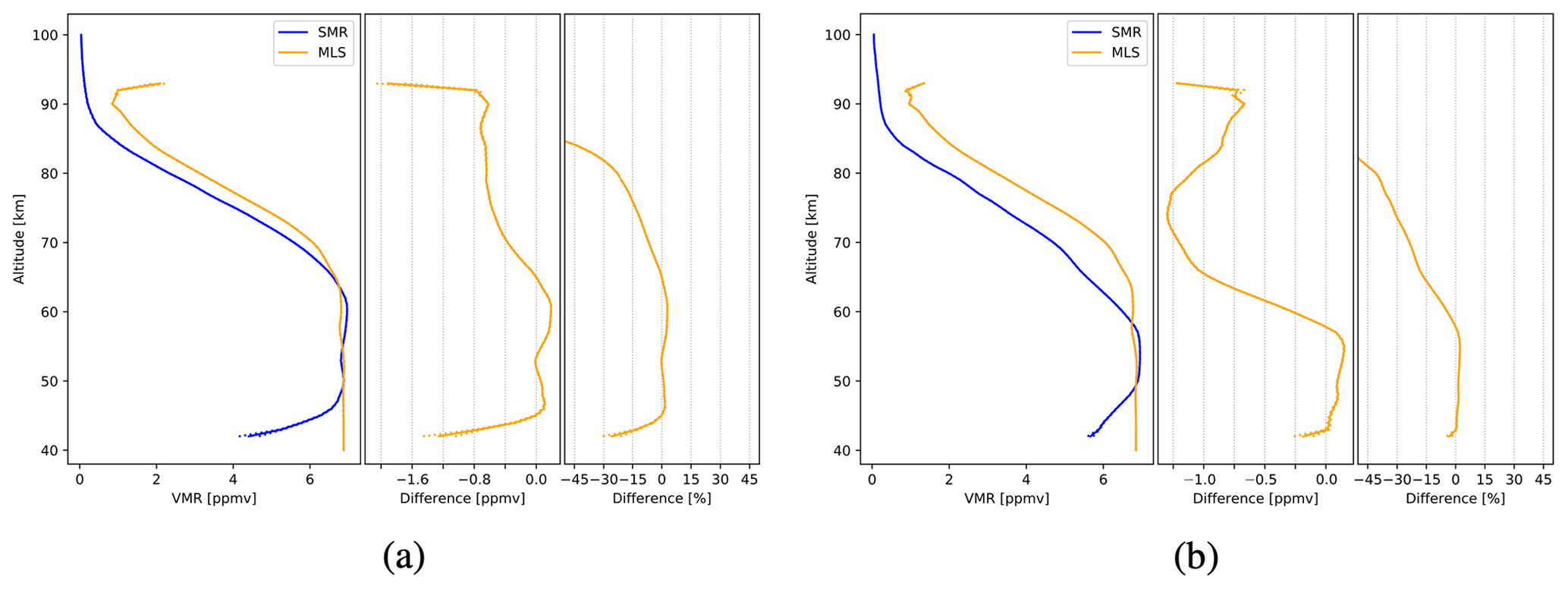
Figure 11Comparison of SMR H2O profiles, from FM13 (a) and FM19 (b), with those from MLS retrievals. The data plotted are global averages over the period between July 2004 and April 2019. Figure characteristics are the same as in Fig. 6.

Figure 12Summary of relative differences of SMR v3.0 H2O concentrations with respect to those from SMR v2.1, as well as those retrieved from measurements by all other instruments considered in this study. For the sake of clarity, errors are not shown. (a) FM13 comparison. (b) FM19 comparison.
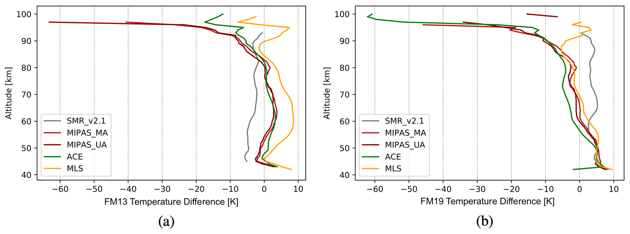
Figure 13Summary of absolute differences of SMR v3.0 temperatures with respect to SMR v2.1 ones as well as those retrieved from measurements by all other instruments considered in this study. For the sake of clarity, errors are not shown. (a) FM13 comparison. (b) FM19 comparison.
The previous version (v2.1) of SMR FM13 and FM19 H2O and temperature products presented large biases compared to other instruments. In particular, FM19 H2O presented a bias between ±20 % between 40 and 80 km, while FM13 concentrations were around 10 % higher than ACE-FTS and MLS between 40 and 60 km, and around 20 % higher than MIPAS in the same altitude range. Above 80 km, both FMs presented differences greater than −50 %. FM19 temperature had a bias of around −5 to −10 K between 60 and 80 km, and FM13 temperature bias was equal to around +10 K between 40 and 80 km. Both FMs were characterized by very high negative biases at high altitudes. After investigating different possible causes, an underestimation of leakage of the image sidebands in the nominally single-sideband receivers was identified as the most likely cause of the majority of these biases. A lower suppression has therefore been assumed and retrievals with the new settings have been performed. This resulted in a new data set (v3.0) covering 18 years of observations from 40 to 100 km altitude, across all latitudes. Time series of H2O mixing ratio and temperature show temporal variation patterns that are consistent with the current knowledge of mesospheric water vapour and temperature, including reasonable signatures of the semi-annual oscillation and annual cycle for example. The validation study, performed by comparing SMR observations with independent satellite measurements from MIPAS, ACE-FTS and MLS, shows that globally averaged SMR v3.0 FM13 H2O concentrations (Fig. 12a) present relative differences within ±20 % between 45 and 80 km altitude. In particular, SMR is in very good agreement with ACE-FTS and MLS up to 70 km, with relative differences within 0 % and −5 %. Relative differences between v3.0 FM19 and all instruments are within ±20 % between 40 and 70 km. In particular, differences with regards to the different MIPAS observation modes are within ±10 % up to 80 km (Fig. 12b). For both FMs, outside the above-mentioned altitude ranges, relative differences reach highly negative values, to a minimum of −140 %. These large relative differences are to be expected due to the fact that H2O mixing ratio values are very low at higher altitudes. It can also be seen that for SMR v3.0 FM19, between 40 and 60 km, there is a general reduction of the relative difference with respect to all other instruments, compared to v2.1. This consists of a few percent with respect to MLS and reaches 10 %–15 % with respect to MIPAS MA and UA modes. Moreover, temperature shows an improvement of about 5 K in absolute difference at all observed altitudes with respect to the previous version for both FMs (Fig. 13). Only FM19 in the 40–60 km altitude range is an exception, where v2.1 agreed better with the other instruments. Temperature from v3.0 FM13 agrees very well with all MIPAS modes and with ACE-FTS between 40 and 85 km, presenting absolute differences within ±3 K. In the same altitude range, SMR-MLS difference however oscillates between +8 and 0 K. SMR v3.0 FM19 temperature absolute difference from all other instruments is equal to +8 K at 40 km and gradually decreases to reach −8 K at 85 km. For both FMs, altitudes above 85 km are characterized by lower absolute differences with respect to almost all instruments, reaching −60 K at 100 km. SMR–MLS difference is an exception, with a value between ±8 K at these altitudes.
The global mesospheric water vapour and temperature data from Odin/SMR have been reprocessed, leading to a significant improvement of the L2 products. The data sets are available to the scientific community at https://odin.rss.chalmers.se/dataaccess (last access: 24 August 2021). They represent valuable tools for the study of middle atmospheric chemistry and dynamics, as well as for trend studies, given their important time coverage (more than 18 years).
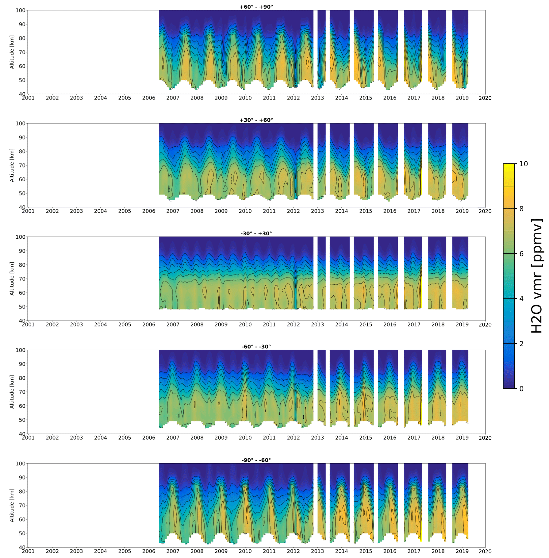
Figure A1Time series of FM13 H2O volume mixing ratios measured by SMR for different latitude bands. The white areas indicate periods and altitudes at which the number of measurements in the given latitude band is lower than 10. The ticks on the x axis correspond to the beginning of each year.
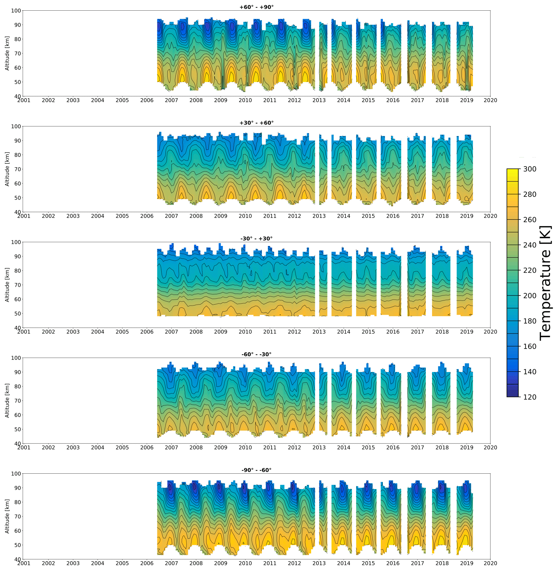
Figure A2Time series of FM13 temperature measured by SMR for different latitude bands. The white areas indicate periods and altitudes at which the number of measurements in the given latitude band is lower than 10. The ticks on the x axis correspond to the beginning of each year.
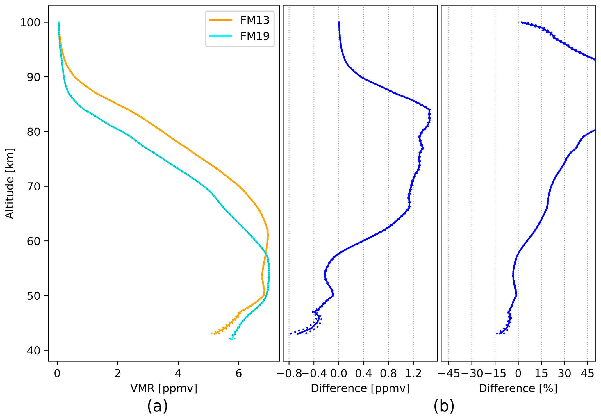
Figure A3Absolute differences (a) and relative differences (b) between SMR v3.0 FM13 and FM19 H2O concentrations. The data plotted are global averages over the whole time period between February 2001 and April 2019.
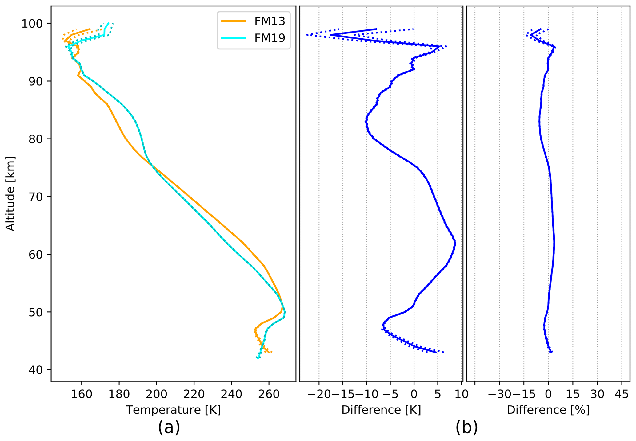
Figure A4Absolute differences (a) and relative differences (b) between SMR v3.0 FM13 and FM19 temperatures. The data plotted are global averages over the whole time period between February 2001 and April 2019.
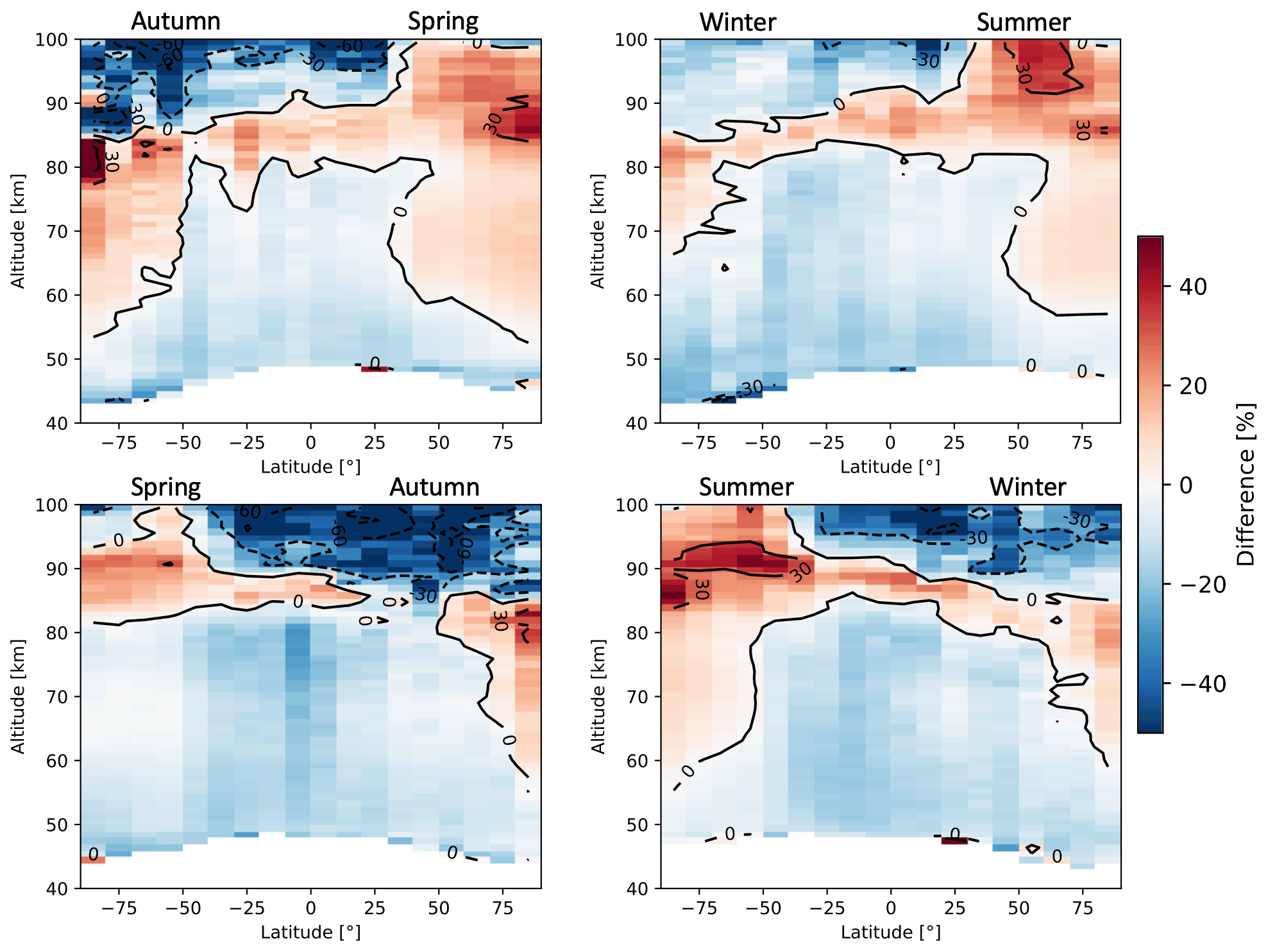
Figure A5Seasonal zonal means of H2O FM13 SMR v3.0–v2.1 relative differences averaged over the whole time period between February 2001 and April 2019. The seasons are intended as astronomical seasons, i.e. each starting at the respective solstice or equinox.
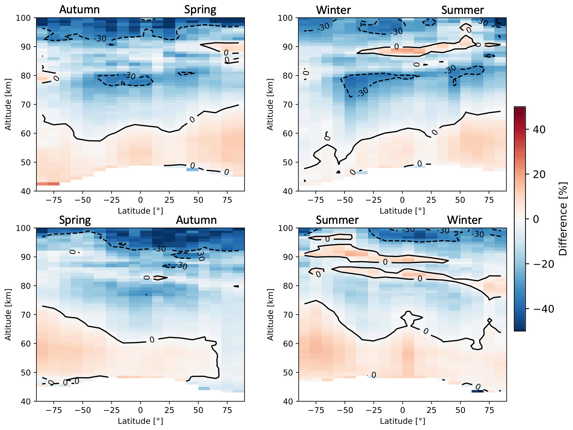
Figure A6Seasonal zonal means of H2O FM19 SMR v3.0–v2.1 relative differences averaged over the whole time period between February 2001 and April 2019. The seasons are intended as astronomical seasons, i.e. each starting at the respective solstice or equinox.
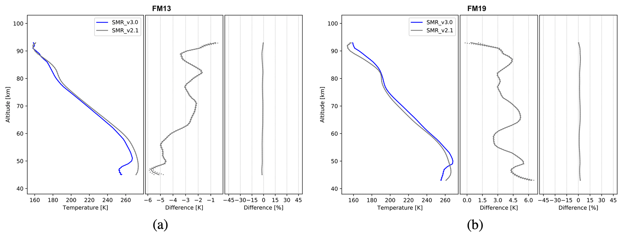
Figure A7Comparison of SMR v3.0 and v2.1 temperatures from FM13 (a) and FM19 (b). The data plotted are global averages over the time period between February 2001 and April 2019. Figure characteristics are the same as in Fig. 6.

Figure A8Seasonal zonal means of temperature FM13 SMR v3.0–v2.1 relative differences averaged over the whole time period between February 2001 and April 2019. The seasons are intended as astronomical seasons, i.e. each starting at the respective solstice or equinox.
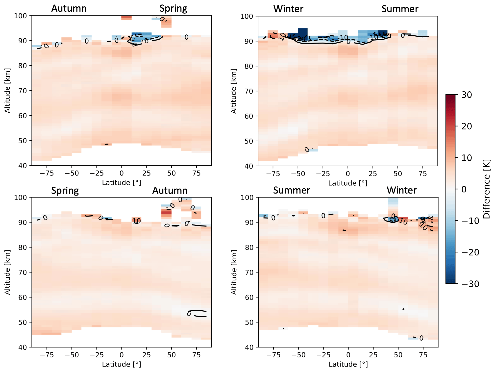
Figure A9Seasonal zonal means of temperature FM19 SMR v3.0–v2.1 relative differences averaged over the whole time period between February 2001 and April 2019. The seasons are intended as astronomical seasons, i.e. each starting at the respective solstice or equinox.
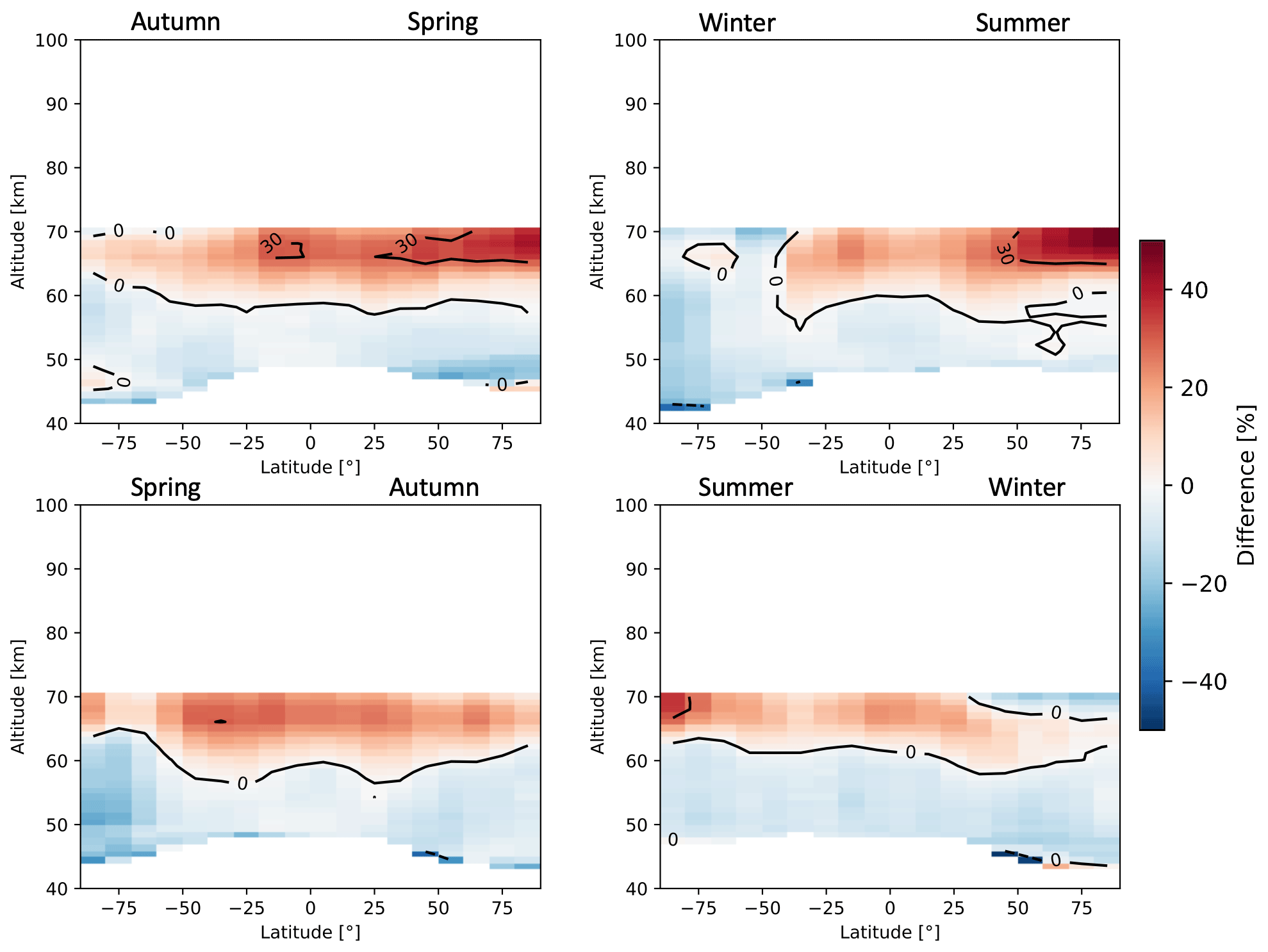
Figure A10Seasonal zonal means of H2O FM13 SMR–MIPAS nominal relative differences averaged over the time period indicated in Table 2. The seasons are intended as astronomical seasons, i.e. each starting at the respective solstice or equinox.

Figure A11Seasonal zonal means of H2O FM19 SMR–MIPAS nominal relative differences averaged over the time period indicated in Table 2. The seasons are intended as astronomical seasons, i.e. each starting at the respective solstice or equinox.
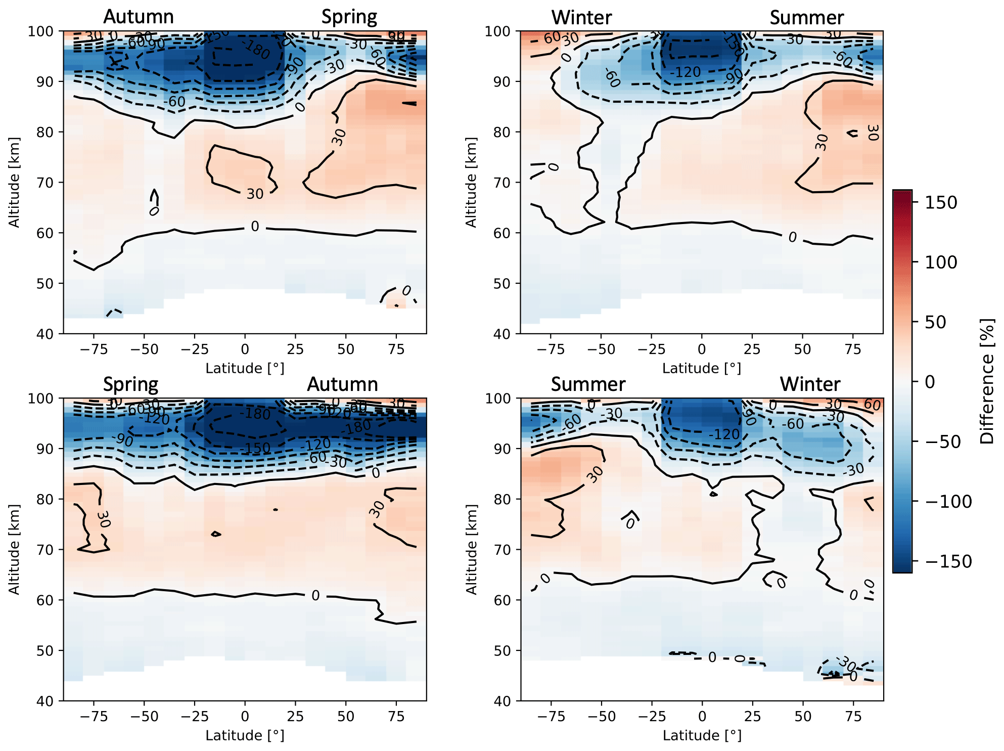
Figure A12Seasonal zonal means of H2O FM13 SMR–MIPAS middle atmosphere relative differences averaged over the time period indicated in Table 2. The seasons are intended as astronomical seasons, i.e. each starting at the respective solstice or equinox.
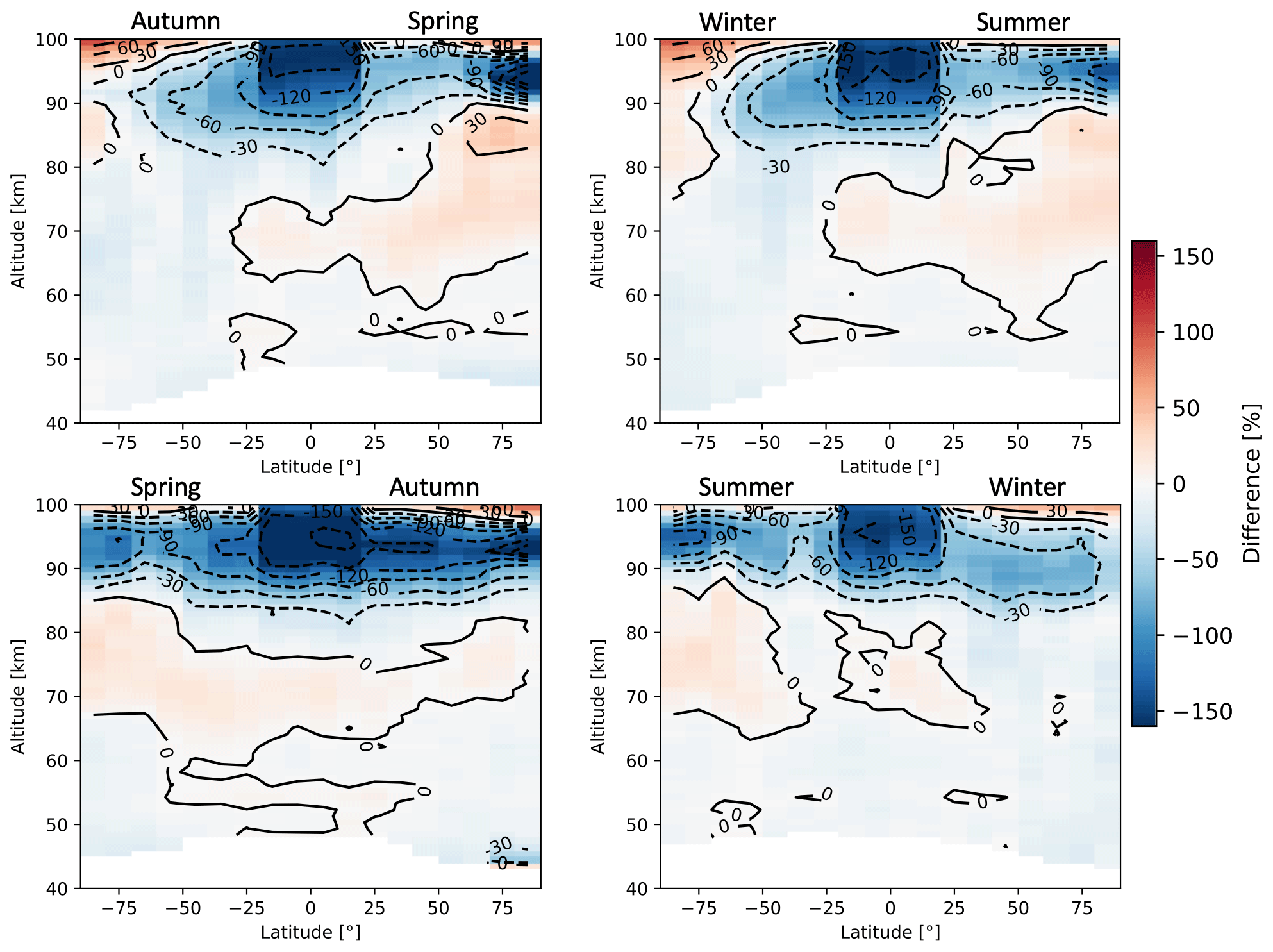
Figure A13Seasonal zonal means of H2O FM19 SMR–MIPAS middle atmosphere relative differences averaged over the time period indicated in Table 2. The seasons are intended as astronomical seasons, i.e. each starting at the respective solstice or equinox.
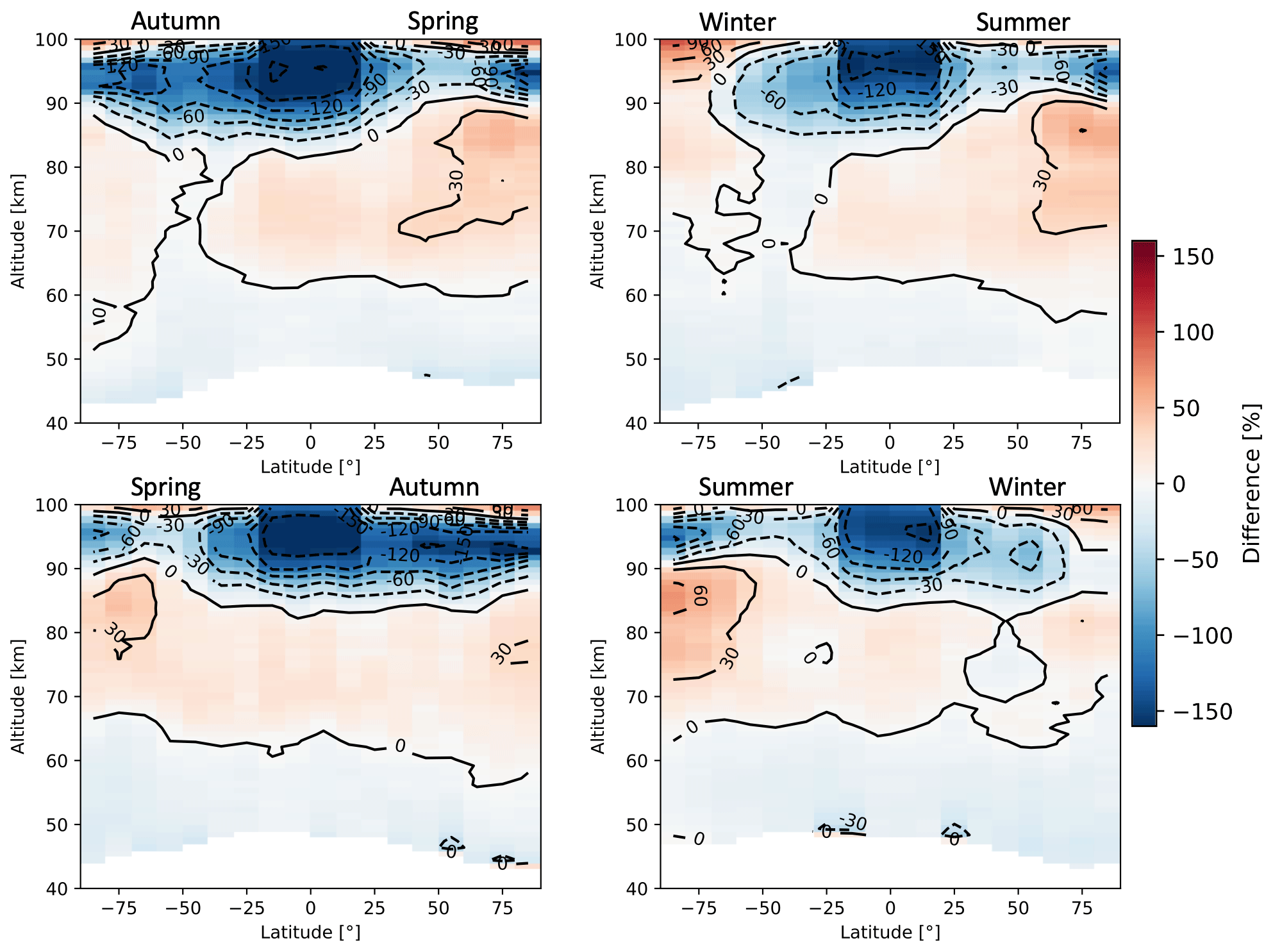
Figure A14Seasonal zonal means of H2O FM13 SMR–MIPAS upper atmosphere relative differences averaged over the time period indicated in Table 2. The seasons are intended as astronomical seasons, i.e. each starting at the respective solstice or equinox.
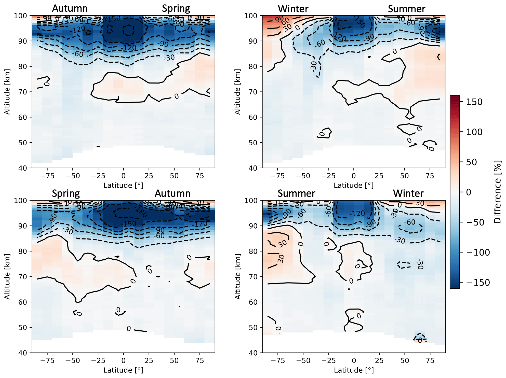
Figure A15Seasonal zonal means of H2O FM19 SMR–MIPAS upper atmosphere relative differences averaged over the time period indicated in Table 2. The seasons are intended as astronomical seasons, i.e. each starting at the respective solstice or equinox.

Figure A16Seasonal zonal means of H2O FM13 SMR–ACE relative differences averaged over the time period between February 2004 and April 2019. The seasons are intended as astronomical seasons, i.e. each starting at the respective solstice or equinox.
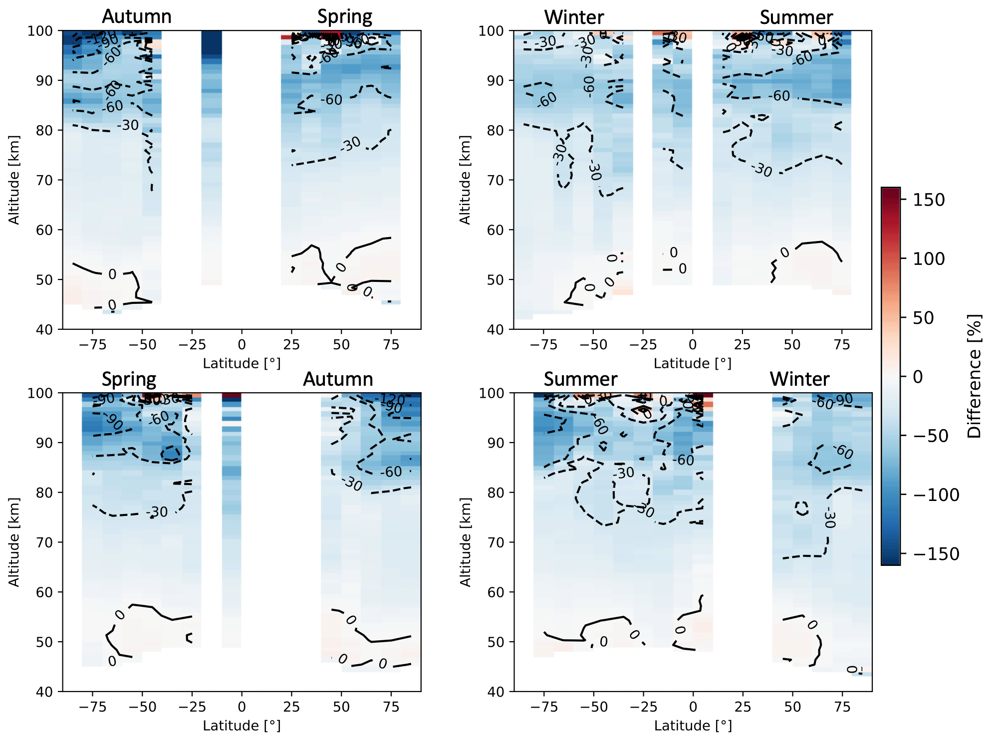
Figure A17Seasonal zonal means of H2O FM19 SMR–ACE relative differences averaged over the time period between February 2004 and April 2019. The seasons are intended as astronomical seasons, i.e. each starting at the respective solstice or equinox.
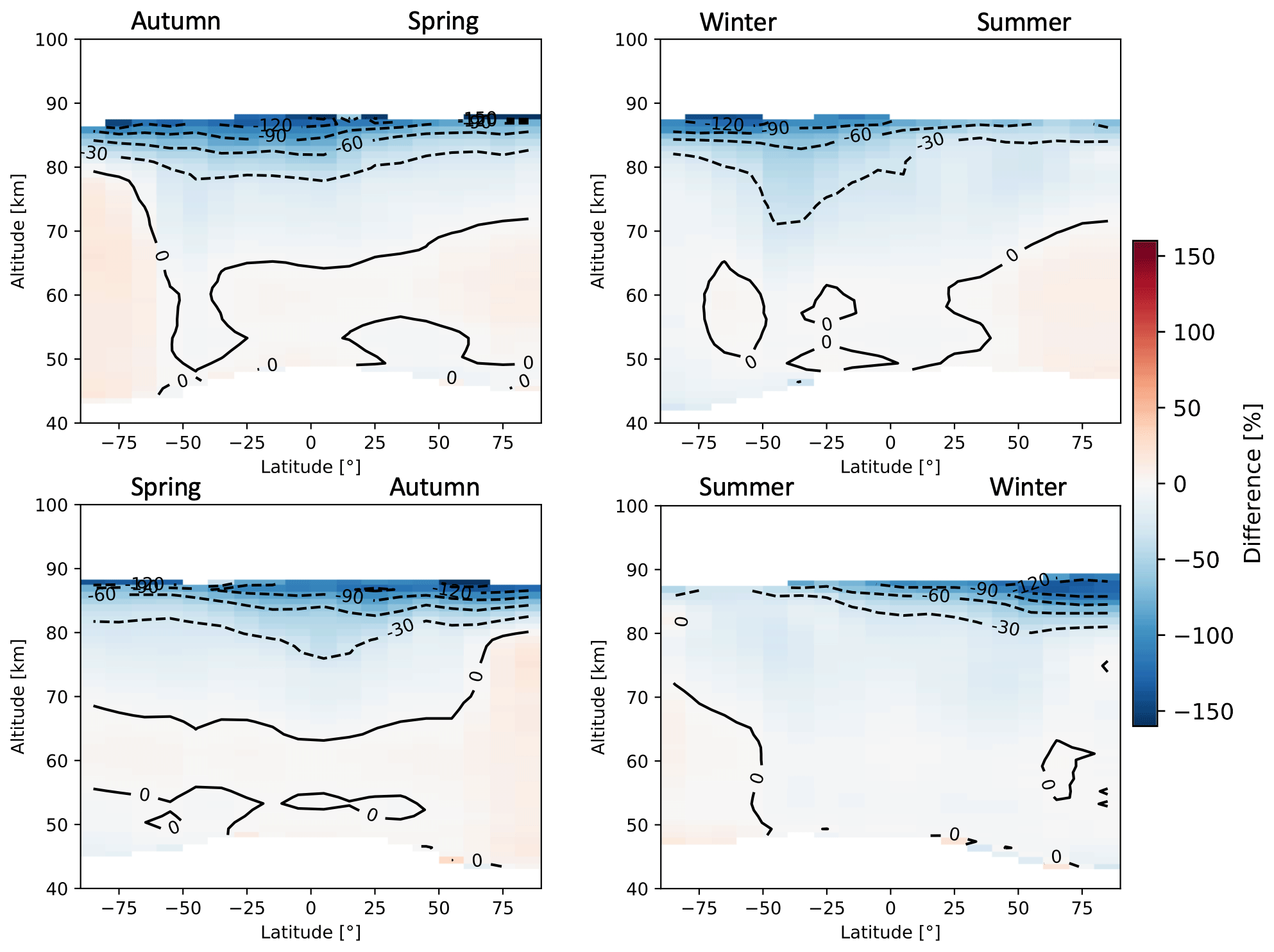
Figure A18Seasonal zonal means of H2O FM13 SMR–MLS relative differences averaged over the time period between July 2004 and April 2019. The seasons are intended as astronomical seasons, i.e. each starting at the respective solstice or equinox.

Figure A19Seasonal zonal means of H2O FM19 SMR–MLS relative differences averaged over the time period between July 2004 and April 2019. The seasons are intended as astronomical seasons, i.e. each starting at the respective solstice or equinox.
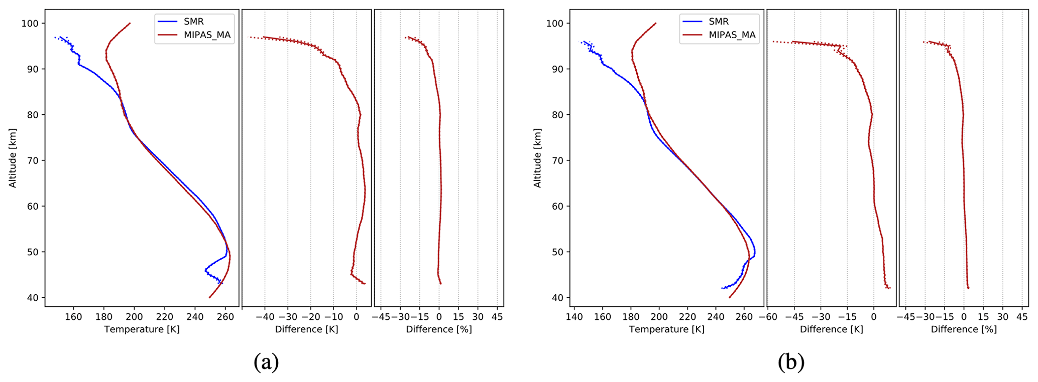

Figure A21Seasonal zonal means of temperature FM13 SMR–MIPAS middle atmosphere absolute differences averaged over the time period indicated in Table 2. The seasons are intended as astronomical seasons, i.e. each starting at the respective solstice or equinox.
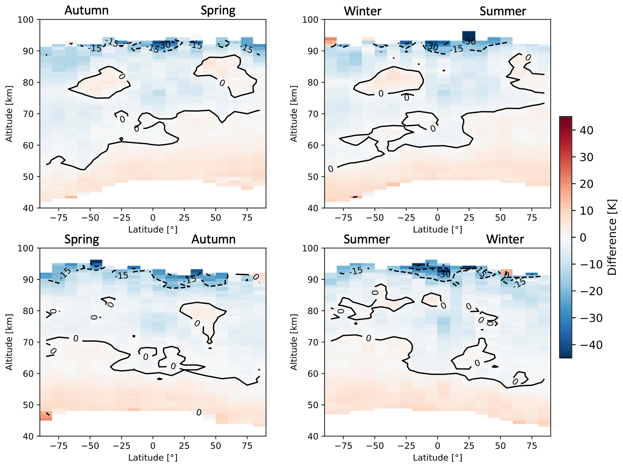
Figure A22Seasonal zonal means of temperature FM19 SMR–MIPAS middle atmosphere absolute differences averaged over the time period indicated in Table 2. The seasons are intended as astronomical seasons, i.e. each starting at the respective solstice or equinox.
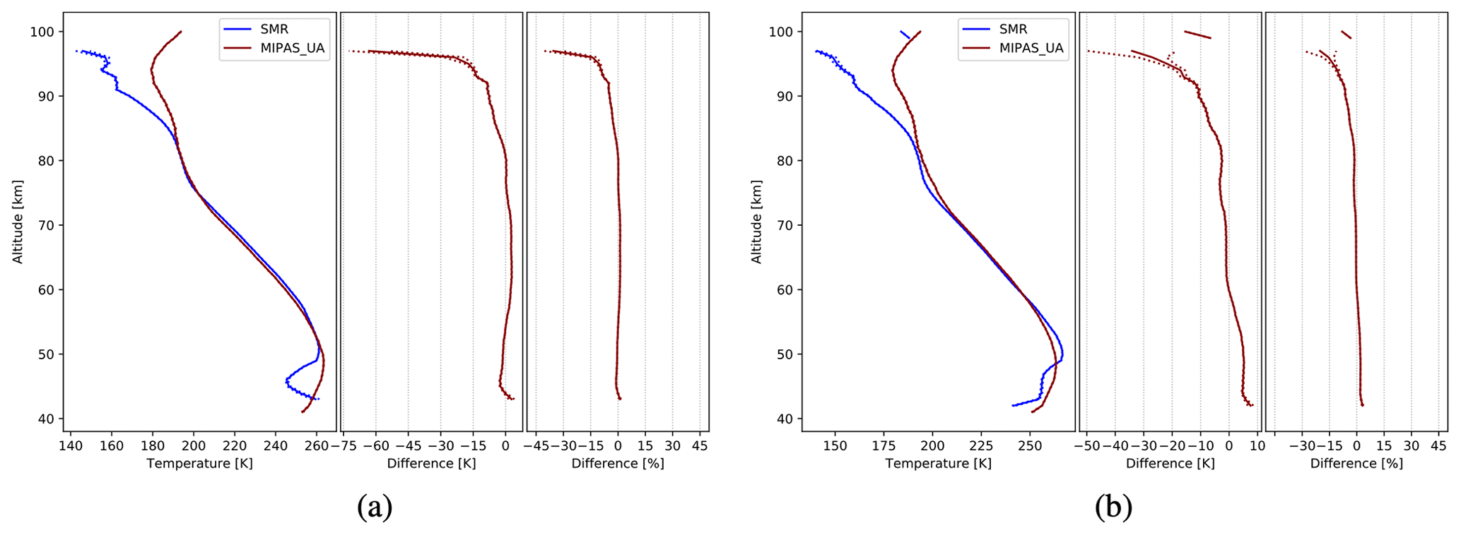
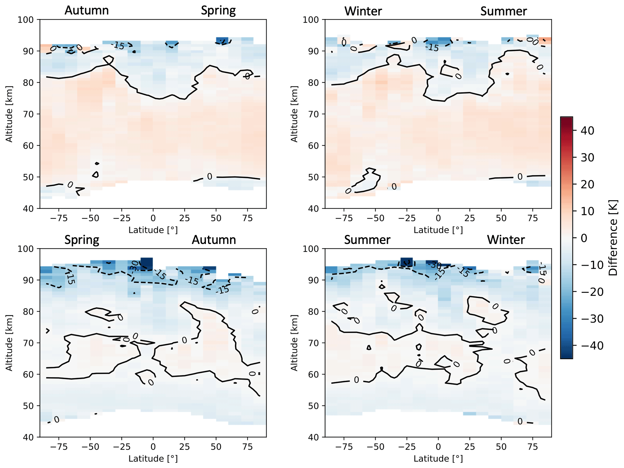
Figure A24Seasonal zonal means of temperature FM13 SMR–MIPAS upper atmosphere absolute differences averaged over the time period indicated in Table 2. The seasons are intended as astronomical seasons, i.e. each starting at the respective solstice or equinox.
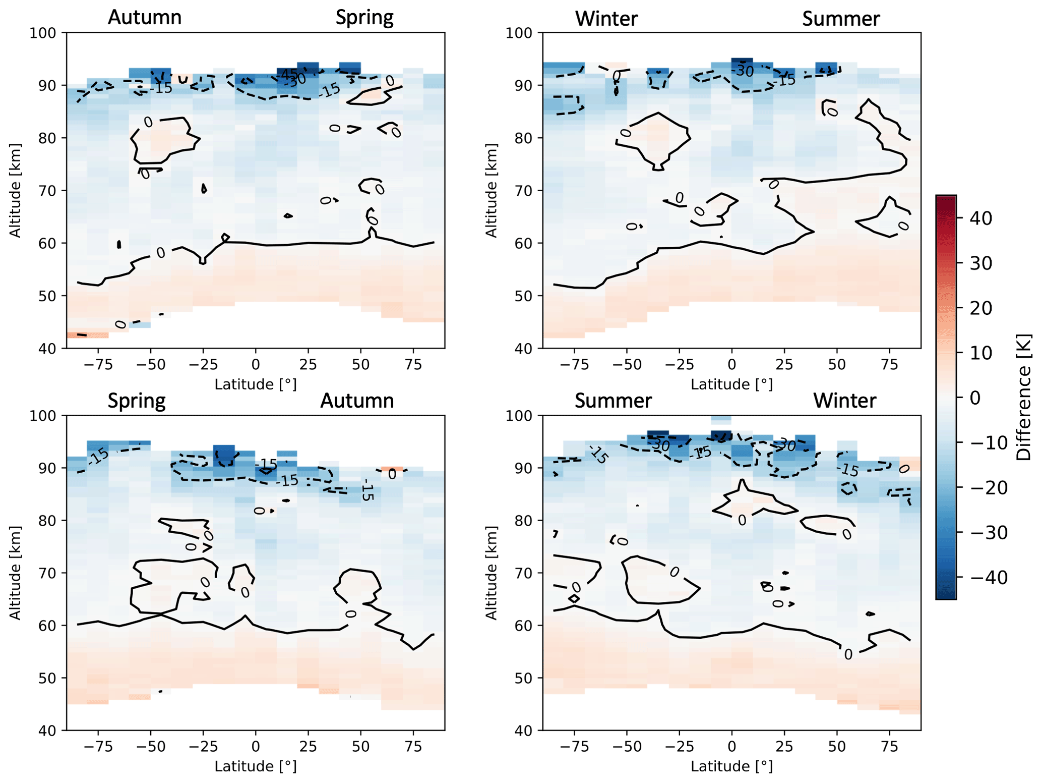
Figure A25Seasonal zonal means of temperature FM19 SMR–MIPAS upper atmosphere absolute differences averaged over the time period indicated in Table 2. The seasons are intended as astronomical seasons, i.e. each starting at the respective solstice or equinox.
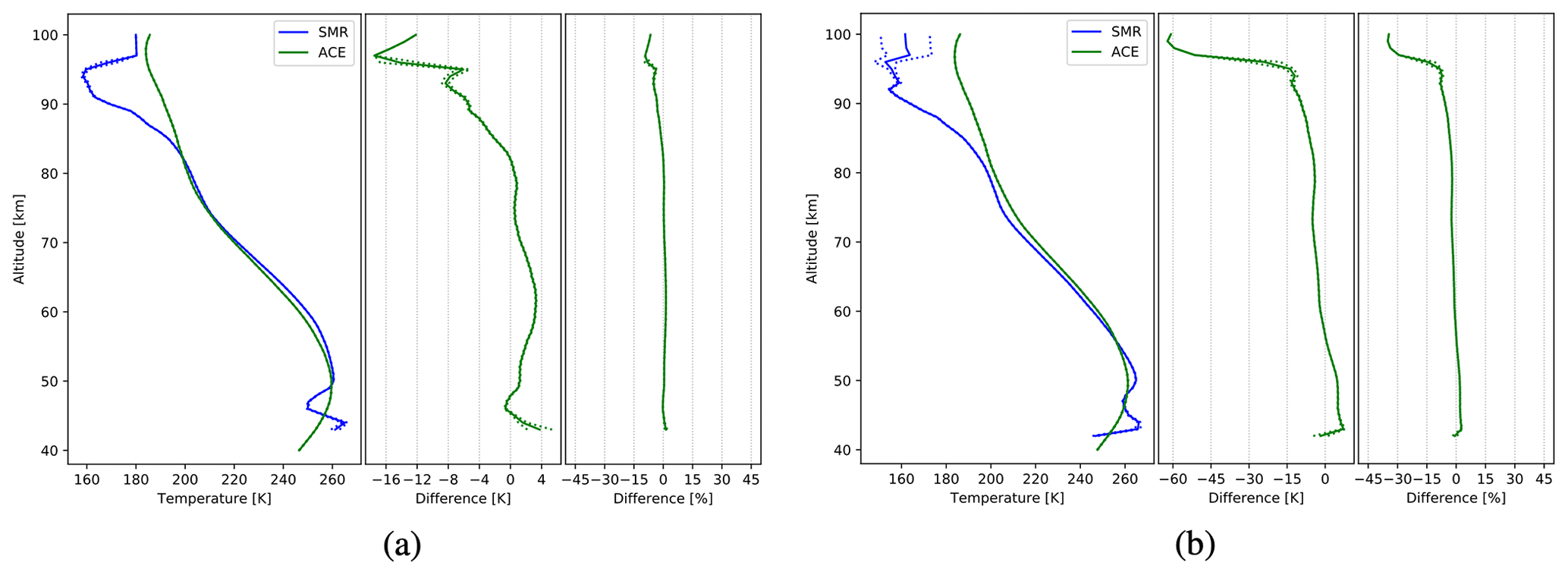
Figure A26Comparison of SMR temperatures, from FM13 (a) and FM19 (b), with those from ACE-FTS retrievals. The data plotted are global averages over the time period between February 2004 and April 2019. Figure characteristics are the same as in Fig. 6.
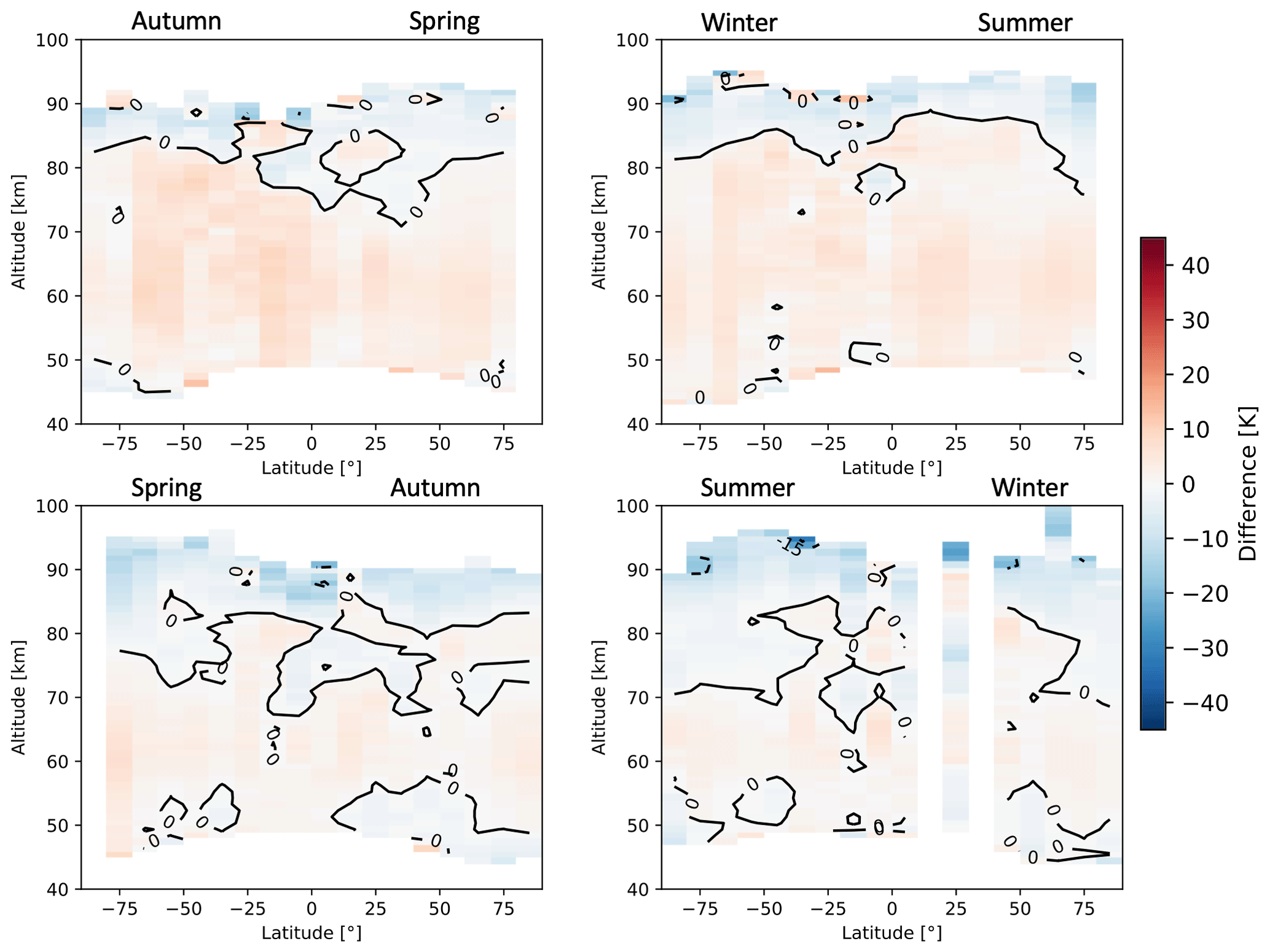
Figure A27Seasonal zonal means of temperature FM13 SMR–ACE absolute differences averaged over the time period between February 2004 and April 2019. The seasons are intended as astronomical seasons, i.e. each starting at the respective solstice or equinox.
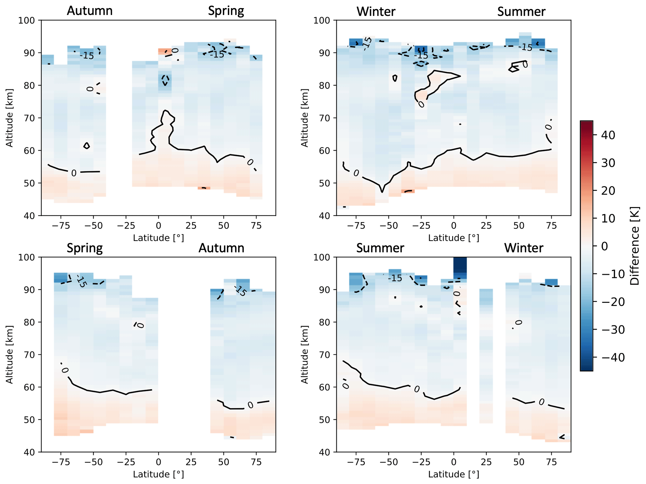
Figure A28Seasonal zonal means of temperature FM19 SMR–ACE absolute differences averaged over the time period between February 2004 and April 2019. The seasons are intended as astronomical seasons, i.e. each starting at the respective solstice or equinox.
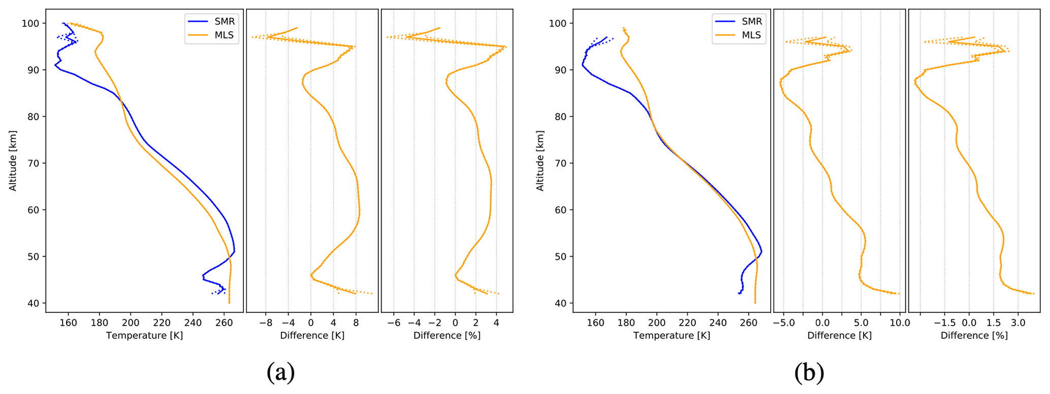
Figure A29Comparison of SMR temperatures, from FM13 (a) and FM19 (b), with those from MLS retrievals. The data plotted are global averages over the time period between July 2004 and April 2019. Figure characteristics are the same as in Fig. 6.
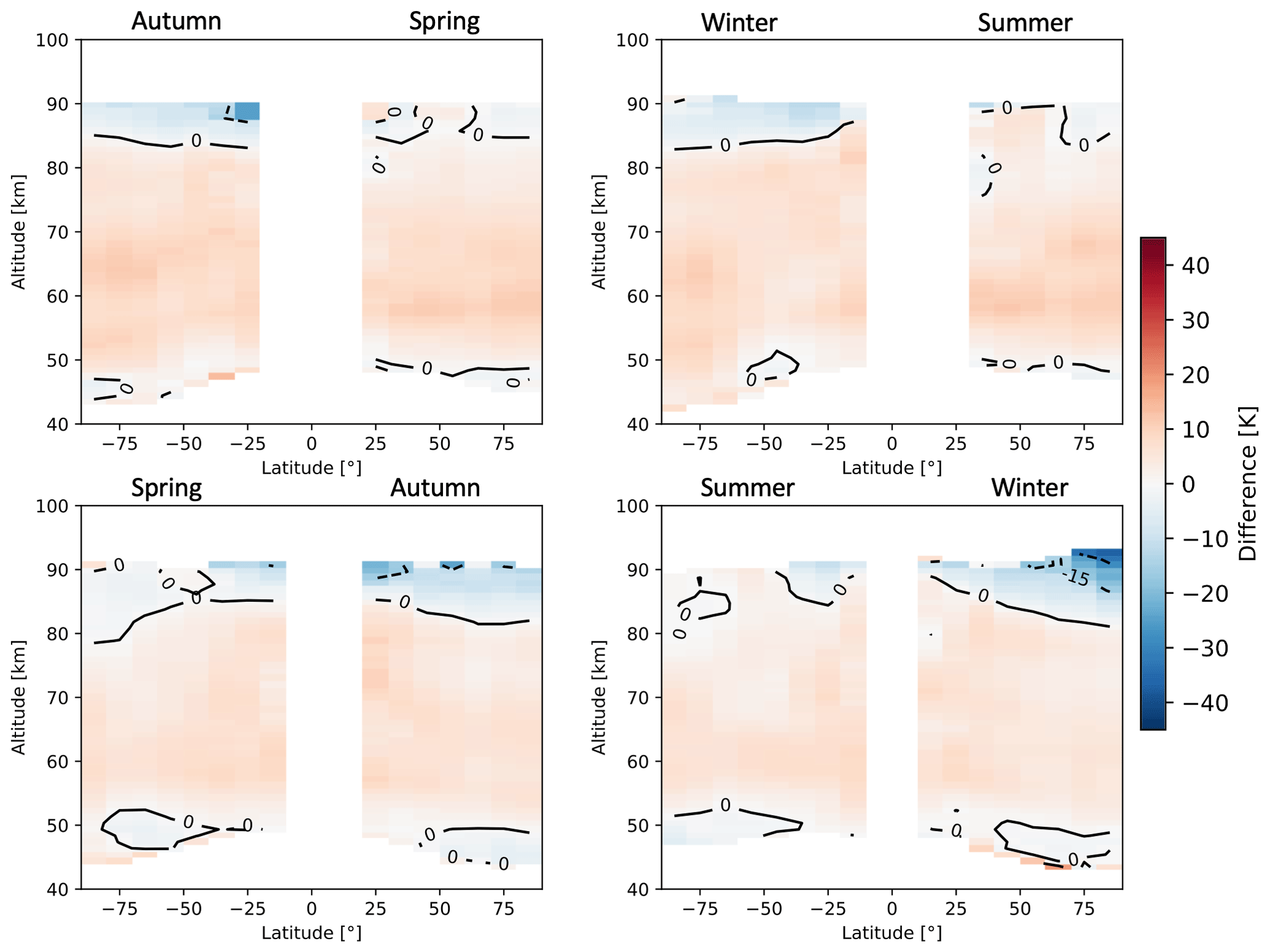
Figure A30Seasonal zonal means of temperature FM13 SMR–MLS absolute differences averaged over the time period between July 2004 and April 2019. The seasons are intended as astronomical seasons, i.e. each starting at the respective solstice or equinox.
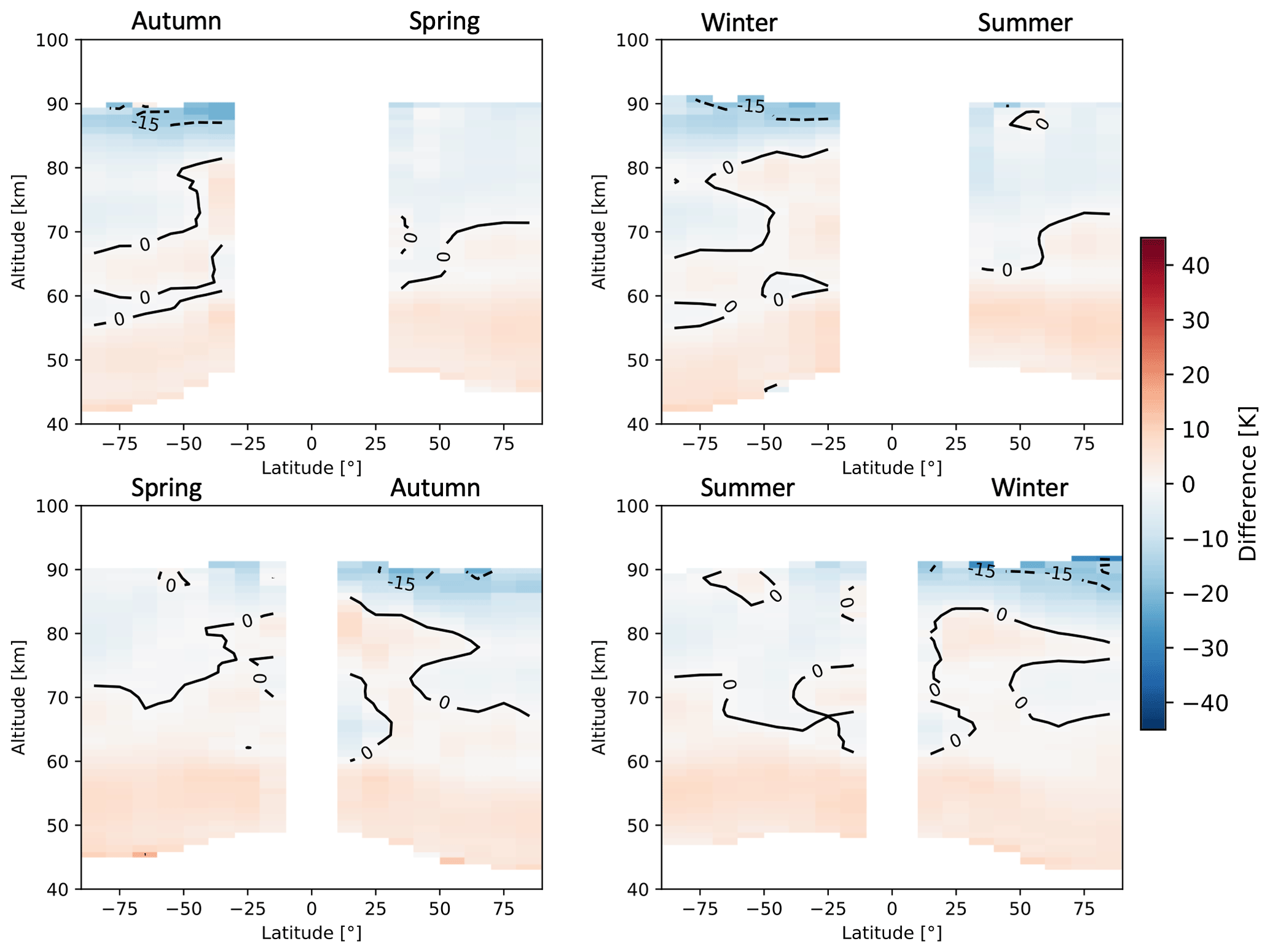
Figure A31Seasonal zonal means of temperature FM19 SMR–MLS absolute differences averaged over the time period between July 2004 and April 2019. The seasons are intended as astronomical seasons, i.e. each starting at the respective solstice or equinox.
More than 18 years of Odin/SMR v3.0 L2 data are publicly accessible at http://odin.rss.chalmers.se/level2 (last access: 24 August 2021; OdinSMR, 2021); MIPAS IMK/IAA L2 data (both NOM and MA/UA) can be downloaded upon registration at http://www.imk-asf.kit.edu/english/308.php (last access: 24 August 2021; KIT, 2021); ACE-FTS L2 data are available upon request at https://databace.scisat.ca/l2signup.php (last access: 24 August 2021; ACE/SCISAT, 2021); MLS v5 H2O L2 data are available at https://doi.org/10.5067/Aura/MLS/DATA2508 (Lambert et al., 2020) and temperature L2 data are available at https://doi.org/10.5067/Aura/MLS/DATA2520 (Schwartz et al., 2020).
FG improved and processed the H2O and T data, made most of the plots and wrote most of the text. KP, DM and PE initiated the project and supported FG throughout it. KP contributed to the writing of the text. BR helped with the processing of the data. All co-authors contributed to the interpretation of the results and proofread the text. In particular, MK and MGC did so by focusing especially on sections relative to MIPAS; AL focusing on MLS sections; KAW focusing on ACE sections.
The authors declare that they have no conflict of interest.
Publisher’s note: Copernicus Publications remains neutral with regard to jurisdictional claims in published maps and institutional affiliations.
This article is part of the special issue “New developments in atmospheric limb measurements: instruments, methods, and science applications (AMT/ACP inter-journal SI)”. It is a result of the 10th international limb workshop, Greifswald, Germany, 4–7 June 2019.
The Chalmers team acknowledges support from the Swedish National Space Agency. Odin is a Swedish-led satellite mission, and is also part of the European Space Agency's (ESA) third-party mission programme. The reprocessing of the SMR data was supported by ESA (MesosphEO and Odin/SMR reprocessing projects). The Atmospheric Chemistry Experiment is a Canadian-led mission mainly supported by the Canadian Space Agency. Work at the Jet Propulsion Laboratory, California Institute of Technology, was carried out under a contract with the National Aeronautics and Space Administration.
This research has been supported by the Swedish National Space Agency (grant nos. 72/17 and 88/14).
This paper was edited by Christian von Savigny and reviewed by two anonymous referees.
ACE/SCISAT: ACE/SCISAT Database, Level 2 Data Access, available at: https://databace.scisat.ca/l2signup.php, last access: 24 August 2021. a
Azeem, S., Palo, S., Wu, D., and Froidevaux, L.: Observations of the 2-day wave in UARS MLS temperature and ozone measurements, Geophys. Res. Lett., 28, 3147–3150, https://doi.org/10.1029/2001GL013119, 2001. a
Brasseur, G. and Solomon, S.: Aeronomy of the Middle Atmosphere, 3rd edition, Springer, Dordrecht, the Netherlands, 2005. a, b
Charlton, A. and Polvani, L.: A New Look at Stratospheric Sudden Warmings. Part I: Climatology and Modeling Benchmarks, J. Climate, 20, 449–469, https://doi.org/10.1175/JCLI3996.1, 2007. a
Christensen, O. M., Benze, S., Eriksson, P., Gumbel, J., Megner, L., and Murtagh, D. P.: The relationship between polar mesospheric clouds and their background atmosphere as observed by Odin-SMR and Odin-OSIRIS, Atmos. Chem. Phys., 16, 12587–12600, https://doi.org/10.5194/acp-16-12587-2016, 2016. a
Clancy, R. and Rusch, D.: Climatology and trends of mesospheric (58–90 km) temperatures based upon 1982–1986 SME Limb scattering profiles, J. Geophys. Res.-Atmos., 94, 3377–3393, https://doi.org/10.1029/JD094iD03p03377, 1989. a
Dawkins, E. C. M., Feofilov, A., Rezac, L., Kutepov, A. A., Janches, D., Höffner, J., Chu, X., Lu, X., Mlynczak, M. G., and Russell III, J.: Validation of SABER v2.0 Operational Temperature Data With Ground-Based Lidars in the Mesosphere-Lower Thermosphere Region (75–105 km), J. Geophys. Res.-Atmos., 123, 9916–9934, https://doi.org/10.1029/2018JD028742, 2018. a
Dee, D., Uppala, S., Simmons, A., Berrisford, P., Poli, P., Kobayashi, S., Andrae, U., Balmaseda, M., Balsamo, G., Bauer, P., Bechtold, P., Beljaars, A., van de Berg, L., Bidlot, J., Bormann, N., Delsol, C., Dragani, R., Fuentes, M., Geer, A., Haimberger, L., Healy, S., Hersbach, H., Hólm, E., Isaksen, L., Kållberg, P., Köhler, M., Matricardi, M., McNally, A., Monge‐Sanz, B., Morcrette, J., Park, B., Peubey, C., de Rosnay, P., Tavolato, C., Thépaut, J., and Vitart, F.: The ERA‐Interim reanalysis: configuration and performance of the data assimilation system, Q. J. R. Meteorol. Soc., 137, 553–597, https://doi.org/10.1002/qj.828, 2011. a
Eriksson, P. and Urban, J.: Post launch characterisation of Odin-SMR sideband filter properties, Technical report, Chalmers University of Technology, Gothenburg, Sweden, 2006. a, b, c
Eriksson, P., Buehler, S., Davis, C., Emde, C., and Lemke, O.: ARTS, the atmospheric radiative transfer simulator, version 2, J. Quant. Spectrosc. Rad., 112, 1551–1558, https://doi.org/10.1016/j.jqsrt.2011.03.001, 2011. a
Feofilov, A. G., Kutepov, A. A., Pesnell, W. D., Goldberg, R. A., Marshall, B. T., Gordley, L. L., García-Comas, M., López-Puertas, M., Manuilova, R. O., Yankovsky, V. A., Petelina, S. V., and Russell III, J. M.: Daytime SABER/TIMED observations of water vapor in the mesosphere: retrieval approach and first results, Atmos. Chem. Phys., 9, 8139–8158, https://doi.org/10.5194/acp-9-8139-2009, 2009. a
Fischer, H., Birk, M., Blom, C., Carli, B., Carlotti, M., von Clarmann, T., Delbouille, L., Dudhia, A., Ehhalt, D., Endemann, M., Flaud, J. M., Gessner, R., Kleinert, A., Koopman, R., Langen, J., López-Puertas, M., Mosner, P., Nett, H., Oelhaf, H., Perron, G., Remedios, J., Ridolfi, M., Stiller, G., and Zander, R.: MIPAS: an instrument for atmospheric and climate research, Atmos. Chem. Phys., 8, 2151–2188, https://doi.org/10.5194/acp-8-2151-2008, 2008. a
Frisk, U., Hagström, M., Ala-Laurinaho, J., Andersson, S., Berges, J.-C., Chabaud, J.-P., Dahlgren, M., Emrich, A., Florén, H.-G., Florin, G., Fredrixon, M., Gaier, T., Haas, R., Hirvonen, T., Å. Hjalmarsson, Jakobsson, B., Jukkala, P., Kildal, P. S., Kollberg, E., Lassing, J., Lecacheux, A., Lehikoinen, P., Lehto, A., Mallat, J., Marty, C., Michet, D., Narbonne, J., Nexon, M., Olberg, M., Olofsson, A. O. H., Olofsson, G., Origné, A., Petersson, M., Piironen, P., Pons, R., Pouliquen, D., Ristorcelli, I., Rosolen, C., Rouaix, G., Räisänen, A. V., Serra, G., Sjöberg, F., Stenmark, L., Torchinsky, S., Tuovinen, J., Ullberg, C., Vinterhav, E., Wadefalk, N., Zirath, H., Zimmermann, P., and Zimmermann, R.: The Odin satellite I. Radiometer design and test, Astron. Astrophys., 402, L27–L34, https://doi.org/10.1051/0004-6361:20030335, 2003. a, b
Funke, B., López-Puertas, M., Stiller, G. P., von Clarmann, T., and Höpfner, M.: A new non–LTE Retrieval Method for Atmospheric Parameters From MIPAS–ENVISAT Emission Spectra, Adv. Space Res., 27, 1099–1104, 2001. a
Grieco, F., Pérot, K., Murtagh, D., Eriksson, P., Forkman, P., Rydberg, B., Funke, B., Walker, K. A., and Pumphrey, H. C.: Recovery and validation of Odin/SMR long-term measurements of mesospheric carbon monoxide, Atmos. Meas. Tech., 13, 5013–5031, https://doi.org/10.5194/amt-13-5013-2020, 2020. a
Hamilton, K.: Middle Atmosphere – Semiannual Oscillation, in: Encyclopedia of Atmospheric Sciences (Second Edition), Academic Press, Oxford, UK, second edition, 26–29, https://doi.org/10.1016/B978-0-12-382225-3.00233-4, 2015. a
Hervig, M. E., Russell III, J. M., Gordley, L. L., Drayson, S. R., Stone, K., Thompson, R. E., Gelman, M. E., McDermid, I. S., Hauchecorne, A., Keckhut, P., McGee, T. J., Singh, U. N., and Gross, M. R.: Validation of temperature measurements from the Halogen Occultation Experiment, J. Geophys. Res.-Atmos., 101, 10277–10285, https://doi.org/10.1029/95JD01713, 1996. a
Karlsson, B., Gumbel, J., Stegman, J., Lautier, N., Murtagh, D., and Team, O.: Studies of Noctilucent Clouds by the Odin Satellite, in: Proceedings of the 35th COSPAR Scientific Assembly, 18–25 July 2004, Paris, France, vol. 35, 2004. a
Kiefer, M. and Lossow, S.: MIPAS-IMK/IAA L2 Data ReadMe, FMI-TN-MesosphEO-WP4-003, Version 1.0, Karlsruhe Institute of Technology, Karlsruhe, Germany, 2017. a
Kiefer, M., von Clarmann, T., Funke, B., García-Comas, M., Glatthor, N., Grabowski, U., Kellmann, S., Kleinert, A., Laeng, A., Linden, A., López-Puertas, M., Marsh, D. R., and Stiller, G. P.: IMK/IAA MIPAS temperature retrieval version 8: nominal measurements, Atmos. Meas. Tech., 14, 4111–4138, https://doi.org/10.5194/amt-14-4111-2021, 2021. a
KIT: Available Data, Karlsruhe Institute of Technology, available at: http://www.imk-asf.kit.edu/english/308.php, last access: 24 August 2021. a
Lambert, A., Read, W., and Livesey, N.: MLS/Aura Level 2 Water Vapor (H2O) Mixing Ratio V005, Greenbelt, MD, USA, Goddard Earth Sciences Data and Information Services Center (GES DISC) [data set], https://doi.org/10.5067/Aura/MLS/DATA2508, 2020. a
Livesey, N., Read, W., Wagner, P., Froidevaux, L., Santee, M., Schwartz, M., Lambert, A., Millán Valle, L., Pumphrey, H., Manney, G., Fuller, R., Jarnot, R., Knosp, B., and Lay, R.: Earth Observing System (EOS) Aura Microwave Limb Sounder (MLS) Version 5.0x Level 2 and 3 data quality and description document, Tech. Rep. D-105336 Rev. A, Jet Propulsion Laboratory, California Institute of Technology, Pasadena, California, USA, 2020. a
Lossow, S., Urban, J., Eriksson, P., Murtagh, D., and Gumbel, J.: Critical parameters for the retrieval of mesospheric water vapour and temperature from Odin/SMR limb measurements at 557 GHz, Adv. Space Res., 40, 835–845, https://doi.org/10.1016/j.asr.2007.05.026, 2007. a
Lossow, S., Urban, J., Gumbel, J., Eriksson, P., and Murtagh, D.: Observations of the mesospheric semi-annual oscillation (MSAO) in water vapour by Odin/SMR, Atmos. Chem. Phys., 8, 6527–6540, https://doi.org/10.5194/acp-8-6527-2008, 2008. a
Lossow, S., Urban, J., Schmidt, H., Marsh, D. R., Gumbel, J., Eriksson, P., and Murtagh, D.: Wintertime water vapor in the polar upper mesosphere and lower thermosphere: First satellite observations by Odin submillimeter radiometer, J. Geophys. Res.-Atmos., 114, D10304, https://doi.org/10.1029/2008JD011462, 2009. a
Lossow, S., Khosrawi, F., Nedoluha, G. E., Azam, F., Bramstedt, K., Burrows, John. P., Dinelli, B. M., Eriksson, P., Espy, P. J., García-Comas, M., Gille, J. C., Kiefer, M., Noël, S., Raspollini, P., Read, W. G., Rosenlof, K. H., Rozanov, A., Sioris, C. E., Stiller, G. P., Walker, K. A., and Weigel, K.: The SPARC water vapour assessment II: comparison of annual, semi-annual and quasi-biennial variations in stratospheric and lower mesospheric water vapour observed from satellites, Atmos. Meas. Tech., 10, 1111–1137, https://doi.org/10.5194/amt-10-1111-2017, 2017. a, b
Lossow, S., Khosrawi, F., Kiefer, M., Walker, K. A., Bertaux, J.-L., Blanot, L., Russell, J. M., Remsberg, E. E., Gille, J. C., Sugita, T., Sioris, C. E., Dinelli, B. M., Papandrea, E., Raspollini, P., García-Comas, M., Stiller, G. P., von Clarmann, T., Dudhia, A., Read, W. G., Nedoluha, G. E., Damadeo, R. P., Zawodny, J. M., Weigel, K., Rozanov, A., Azam, F., Bramstedt, K., Noël, S., Burrows, J. P., Sagawa, H., Kasai, Y., Urban, J., Eriksson, P., Murtagh, D. P., Hervig, M. E., Högberg, C., Hurst, D. F., and Rosenlof, K. H.: The SPARC water vapour assessment II: profile-to-profile comparisons of stratospheric and lower mesospheric water vapour data sets obtained from satellites, Atmos. Meas. Tech., 12, 2693–2732, https://doi.org/10.5194/amt-12-2693-2019, 2019. a, b, c
Montoux, N., Hauchecorne, A., Pommereau, J.-P., Lefèvre, F., Durry, G., Jones, R. L., Rozanov, A., Dhomse, S., Burrows, J. P., Morel, B., and Bencherif, H.: Evaluation of balloon and satellite water vapour measurements in the Southern tropical and subtropical UTLS during the HIBISCUS campaign, Atmos. Chem. Phys., 9, 5299–5319, https://doi.org/10.5194/acp-9-5299-2009, 2009. a
Munro, R. and Rodgers, C. D.: Latitudinal and season variations of water vapour in the middle atmosphere, Geophys. Res. Lett., 21, 661–664, https://doi.org/10.1029/94GL00183, 1994. a
Murtagh, D., Skyman, A., Rydberg, B., and Eriksson, P.: Odin/SMR Product Validation and Evolution Report, Technical report, Chalmers University of Technology, Department of Space, Earth and Environment, avaialbe at: http://odin.rss.chalmers.se/static/documents/PVER.pdf (last access: 24 August 2021), 2020. a, b, c, d
Nassar, R., Bernath, P. F., Boone, C. D., Manney, G. L., McLeod, S. D., Rinsland, C. P., Skelton, R., and Walker, K. A.: Stratospheric abundances of water and methane based on ACE-FTS measurements, Geophys. Res. Lett., 32, L15S04, https://doi.org/10.1029/2005GL022383, 2005. a
OdinSMR: Level2 data dashboard, available at: http://odin.rss.chalmers.se/level2, last access: 24 August 2021. a
Oelhaf, H.: MIPAS Mission Plan, Issue 4, Version 3, ESA Technical Note ENVI-SPPA-EOPG-TN-07-0073, Karlsruhe Institute of Technology, Karlsruhe, Germany, 2008. a
Pérot, K., Hauchecorne, A., Montmessin, F., Bertaux, J.-L., Blanot, L., Dalaudier, F., Fussen, D., and Kyrölä, E.: First climatology of polar mesospheric clouds from GOMOS/ENVISAT stellar occultation instrument, Atmos. Chem. Phys., 10, 2723–2735, https://doi.org/10.5194/acp-10-2723-2010, 2010. a
Pérot, K., Urban, J., and Murtagh, D. P.: Unusually strong nitric oxide descent in the Arctic middle atmosphere in early 2013 as observed by Odin/SMR, Atmos. Chem. Phys., 14, 8009–8015, https://doi.org/10.5194/acp-14-8009-2014, 2014. a
Picone, J., Hedin, A., Drob, D., and Aikin, A.: NRLMSISE-00 empirical model of the atmosphere: Statistical comparisons and scientific issues, J. Geophys. Res., 107, 1468, https://doi.org/10.1029/2002JA009430, 2002. a
Randall, C., Rusch, D., Bevilacqua, R., Hoppel, K., Lumpe, J., Shettle, E., Thompson, E., Deaver, L., Zawodny, J., Kyrö, E., Johnson, B., Kelder, H., Dorokhov, V., König‐Langlo, G., and Gil, M.: Validation of POAM III ozone: comparison with ozonesonde and satellite data, J. Geophys. Res., 108, 4367, https://doi.org/10.1029/2002JD002944, 2003. a
Remsberg, E., Russell, J. M., Gordley, L. L., Gille, J. C., and Bailey, P. L.: Implications of the Stratospheric Water Vapor Distribution as Determined from the Nimbus 7 LIMS Experiment, J. Atmos. Sci., 41, 2934–2948, https://doi.org/10.1175/1520-0469(1984)041<2934:IOTSWV>2.0.CO;2, 1984. a
Remsberg, E., Damadeo, R., Natarajan, M., and Bhatt, P.: Observed Responses of Mesospheric Water Vapor to Solar Cycle and Dynamical Forcings, J. Geophys. Res.-Atmos., 123, 3830–3843, https://doi.org/10.1002/2017JD028029, 2018. a
Rodgers, C.: Inverse methods for atmospheric sounding: Theory and practise, 1st edition, World Scientific Publishing, Singapore, 2000. a, b, c
Rong, P., Russell, J. M., Marshall, B. T., Gordley, L. L., Mlynczak, M. G., and Walker, K. A.: Validation of water vapor measured by SABER on the TIMED satellite, J. Atmos. Sol.-Terr. Phy., 194, 105099, https://doi.org/10.1016/j.jastp.2019.105099, 2019. a
Rydberg, B., Eriksson, P., Kiviranta, J., Ringsby, J., Skyman, A., and Murtagh, D.: Odin/SMR Algorithm Theoretical Basis Document: Level 1 Processing, Technical Report, Chalmers University of Technology, Department of Space, Earth and Environment, available at: http://odin.rss.chalmers.se/#documents (last access: 24 August 2021), 2017. a
Schwartz, M., Livesey, N., and Read, W.: MLS/Aura Level 2 Temperature V005, Greenbelt, MD, USA, Goddard Earth Sciences Data and Information Services Center (GES DISC) [data set], https://doi.org/10.5067/Aura/MLS/DATA2520, 2020. a
Schwartz, M. J., Lambert, A., Manney, G. L., Read, W. G., Livesey, N. J., Froidevaux, L., Ao, C. O., Bernath, P. F., Boone, C. D., Cofield, R. E., Daffer, W. H., Drouin, B. J., Fetzer, E. J., Fuller, R. A., Jarnot, R. F., Jiang, J. H., Jiang, Y. B., Knosp, B. W., Krüger, K., Li, J.-L. F., Mlynczak, M. G., Pawson, S., Russell III, J. M., Santee, M. L., Snyder, W. V., Stek, P. C., Thurstans, R. P., Tompkins, A. M., Wagner, P. A., Walker, K. A., Waters, J. W., and Wu, D. L.: Validation of the Aura Microwave Limb Sounder temperature and geopotential height measurements, J. Geophys. Res.-Atmos., 113, D15S11, https://doi.org/10.1029/2007JD008783, 2008. a
Sheese, P. E., Boone, C. D., and Walker, K. A.: Detecting physically unrealistic outliers in ACE-FTS atmospheric measurements, Atmos. Meas. Tech., 8, 741–750, https://doi.org/10.5194/amt-8-741-2015, 2015. a
Sheese, P. E., Walker, K. A., Boone, C. D., Bernath, P. F., Froidevaux, L., Funke, B., Raspollini, P., and von Clarmann, T.: ACE-FTS ozone, water vapour, nitrous oxide, nitric acid, and carbon monoxide profile comparisons with MIPAS and MLS, J. Quant. Spectrosc. Ra., 186, 63–80, https://doi.org/10.1016/j.jqsrt.2016.06.026, 2017. a
Sica, R. J., Izawa, M. R. M., Walker, K. A., Boone, C., Petelina, S. V., Argall, P. S., Bernath, P., Burns, G. B., Catoire, V., Collins, R. L., Daffer, W. H., De Clercq, C., Fan, Z. Y., Firanski, B. J., French, W. J. R., Gerard, P., Gerding, M., Granville, J., Innis, J. L., Keckhut, P., Kerzenmacher, T., Klekociuk, A. R., Kyrö, E., Lambert, J. C., Llewellyn, E. J., Manney, G. L., McDermid, I. S., Mizutani, K., Murayama, Y., Piccolo, C., Raspollini, P., Ridolfi, M., Robert, C., Steinbrecht, W., Strawbridge, K. B., Strong, K., Stübi, R., and Thurairajah, B.: Validation of the Atmospheric Chemistry Experiment (ACE) version 2.2 temperature using ground-based and space-borne measurements, Atmos. Chem. Phys., 8, 35–62, https://doi.org/10.5194/acp-8-35-2008, 2008. a
Sioris, C., Zou, J., McElroy, C., McLinden, C., and Vömel, H.: High vertical resolution water vapour profiles in the upper troposphere and lower stratosphere retrieved from MAESTRO solar occultation spectra, Adv. Space Res., 46, 642–650, https://doi.org/10.1016/j.asr.2010.04.040, 2010. a
Stevens, M. H., Deaver, L. E., Hervig, M. E., Russell III, J. M., Siskind, D. E., Sheese, P. E., Llewellyn, E. J., Gattinger, R. L., Höffner, J., and Marshall, B. T.: Validation of upper mesospheric and lower thermospheric temperatures measured by the Solar Occultation for Ice Experiment, J. Geophys. Res.-Atmos., 117, D16304, https://doi.org/10.1029/2012JD017689, 2012. a
Thomas, G.: Clouds And Fog – Noctilucent Clouds, in: Encyclopedia of Atmospheric Sciences, second edition, edited by: North, G. R., Pyle, J., and Zhang, F., Academic Press, Oxford, UK, 189–195, https://doi.org/10.1016/B978-0-12-382225-3.00243-7, 2015. a
Urban, J., Lautié, N., Murtagh, D., Eriksson, P., Kasai, Y., Lossow, S., Dupuy, E., de La Noë, J., Frisk, U., Olberg, M., Flochmoën, E. L., and Ricaud, P.: Global observations of middle atmospheric water vapour by the Odin satellite: An overview, Planet. Space Sci., 55, 1093–1102, https://doi.org/10.1016/j.pss.2006.11.021, 2007. a, b
Vignon, E. and Mitchell, D.: The stratopause evolution during different types of sudden stratospheric warming event, Clim. Dynam., 44, 3323, https://doi.org/10.1007/s00382-014-2292-4, 2015. a
von Clarmann, T., Höpfner, M., Kellmann, S., Linden, A., Chauhan, S., Funke, B., Grabowski, U., Glatthor, N., Kiefer, M., Schieferdecker, T., Stiller, G. P., and Versick, S.: Retrieval of temperature, H2O, O3, HNO3, CH4, N2O, ClONO2 and ClO from MIPAS reduced resolution nominal mode limb emission measurements, Atmos. Meas. Tech., 2, 159–175, https://doi.org/10.5194/amt-2-159-2009, 2009. a
Waters, J. W., Froidevaux, L., Harwood, R. S., Jarnot, R. F., Pickett, H. M., Read, W. G., Siegel, P. H., Cofield, R. E., Filipiak, M. J., Flower, D. A., Holden, J. R., Lau, G. K., Livesey, N. J., Manney, G. L., Pumphrey, H. C., Santee, M. L., Wu, D. L., Cuddy, D. T., Lay, R. R., Loo, M. S., Perun, V. S., Schwartz, M. J., Stek, P. C., Thurstans, R. P., Boyles, M. A., Chandra, K. M., Chavez, M. C., Gun-Shing Chen, Chudasama, B. V., Dodge, R., Fuller, R. A., Girard, M. A., Jiang, J. H., Yibo Jiang, Knosp, B. W., LaBelle, R. C., Lam, J. C., Lee, K. A., Miller, D., Oswald, J. E., Patel, N. C., Pukala, D. M., Quintero, O., Scaff, D. M., Van Snyder, W., Tope, M. C., Wagner, P. A., and Walch, M. J.: The Earth observing system microwave limb sounder (EOS MLS) on the aura Satellite, IEEE T. Geosci. Remote, 44, 1075–1092, 2006. a
Weigel, K., Rozanov, A., Azam, F., Bramstedt, K., Damadeo, R., Eichmann, K.-U., Gebhardt, C., Hurst, D., Kraemer, M., Lossow, S., Read, W., Spelten, N., Stiller, G. P., Walker, K. A., Weber, M., Bovensmann, H., and Burrows, J. P.: UTLS water vapour from SCIAMACHY limb measurementsV3.01 (2002–2012), Atmos. Meas. Tech., 9, 133–158, https://doi.org/10.5194/amt-9-133-2016, 2016. a
- Abstract
- Introduction
- H2O and temperature measurements
- The new SMR data sets
- Comparison with other instruments
- Summary and conclusions
- Appendix A
- Data availability
- Author contributions
- Competing interests
- Disclaimer
- Special issue statement
- Acknowledgements
- Financial support
- Review statement
- References