the Creative Commons Attribution 4.0 License.
the Creative Commons Attribution 4.0 License.
 | 17 Sep 2021
An algorithm to detect non-background signals in greenhouse gas time series from European tall tower and mountain stations
Alex Resovsky
Michel Ramonet
Leonard Rivier
Jerome Tarniewicz
Philippe Ciais
Martin Steinbacher
Ivan Mammarella
Meelis Mölder
Michal Heliasz
Dagmar Kubistin
Matthias Lindauer
Jennifer Müller-Williams
Sebastien Conil
Richard Engelen
We present a statistical framework to identify regional signals in station-based CO2 time series with minimal local influence. A curve-fitting function is first applied to the detrended time series to derive a harmonic describing the annual CO2 cycle. We then combine a polynomial fit to the data with a short-term residual filter to estimate the smoothed cycle and define a seasonally adjusted noise component, equal to 2 standard deviations of the smoothed cycle about the annual cycle. Spikes in the smoothed daily data which surpass this ±2σ threshold are classified as anomalies. Examining patterns of anomalous behavior across multiple sites allows us to quantify the impacts of synoptic-scale atmospheric transport events and better understand the regional carbon cycling implications of extreme seasonal occurrences such as droughts.
- Article
(3373 KB) - Full-text XML
- BibTeX
- EndNote


Continuous measurements of long-lived atmospheric greenhouse gases (GHGs) at ground-based monitoring stations exhibit variations at multiple timescales. These include a well-established diurnal cycle and an annual pattern linked to seasonality which generally exist on top of the long-term trend of the background concentration. Other variations, related to localized surface fluxes or regional-scale atmospheric transport patterns, are observable at synoptic frequencies lasting from 1–2 d to several weeks, while others reflect longer-term meteorological occurrences such as droughts or ocean circulation anomalies. Identification of these latter components can reveal much about the intensity and geographic extent of specific atmospheric events while also improving understanding of background signal evolution. Extracting them, however, requires a methodology to decompose the signal into “background” and “non-background” components and to differentiate meteorology-driven regional signals from spikes due to local emissions, biospheric uptake and other forms of signal noise.
We define “background” here as “the concentration of a given species in a pristine air mass in which anthropogenic impurities of a relatively short lifetime are not present” (IUPAC, 1997). Various methods exist to extract background signals in atmospheric time series. These include back-trajectory analyses that categorize readings based on air provenance (e.g., Schuepbach et al., 2001; Balzani Loöv et al., 2008; Cui et al., 2011) and the application of chemical filters using markers such as 222Rn (e.g., Biraud et al., 2000; Pal et al., 2015; Chambers et al., 2016) or NOy and CO (e.g., Parrish et al., 1991; Zellweger et al., 2003). Although such approaches yield reliable estimates, they are often labor-intensive or require sophisticated transport modeling or additional instrumentation and must take into account site-specific measurement conditions and data availability. Statistical algorithms provide high-precision, computationally inexpensive alternatives to these techniques. These commonly involve a two- or three-step process in which data are first smoothed using filters or polynomial curve fitting then subsequently refined through the identification of outliers, characterized as points which deviate from the curve by more than a specified threshold (e.g., ±σ, ±2σ, or ±3σ, where σis the standard deviation of the residuals about a smooth curve fit to the data).
Already in the late 1980s, Thoning et al. (1989) developed a filtering technique to separate the annual cycle from the long-term trend and approximate the background signal of the CO2 record at Mauna Loa (Hawaii). More recently, O'Doherty et al. (2001) extracted non-background components of atmospheric CHCl3 time series by fitting a polynomial to the daily minima of a moving 121 d span of measurements. They then subtracted the polynomial fit from the data and estimated σ from the measurements below the median of the residual distribution. Measurements on the middle day of each 121 d period exceeding ±3σ were flagged as “polluted” and removed. In a second iteration, readings between ±2σ and ±3σ above the median of the newly refined residual set were marked as “possibly polluted” and subsequently removed if immediately adjacent to “polluted” data points. Giostra et al. (2011) applied a similar approach to atmospheric halocarbon records. They calculated a probability density function (PDF) using the deviations of all data points from σ, predefined as the 16th percentile of measurements within a 30 d span. A Gaussian curve was then defined using σ and the median value of the PDF, and a Gamma curve was fit such that the sum of the two curves yielded a best-fit to the PDF. The background was approximated using all data points below the intersection of the Gamma curve and the right-hand branch of the Gaussian curve. Ruckstuhl et al. (2012) estimated background signals in atmospheric CO and HFC-152a series by applying a localized linear regression to a given span of data points and removing points which deviated by more than the σ value of the negative (left side) residuals within each successive, overlapping span. Individual points were then weighted for robustness according to their distance from the newly defined background curve, with iterative applications further refining the dataset. Apadula et al. (2019) developed an algorithm to subtract outliers from hourly CO2 datasets. They first removed all values which differed by more than a specified threshold ρ from the median value within a sliding 21 d window and subsequently rejected values that differed by more than ρ from the mean value of the remaining points.
Such methods have been widely applied to estimate baseline concentrations of atmospheric trace gases and, in some instances, to identify the occurrence of short-term signal spikes in time series (e.g., El Yazidi et al., 2018). Lacking in the current literature, however, is a comprehensive statistical framework for the extraction of non-background events occurring at synoptic (1–2 d to several weeks) to seasonal timescales. We thus present here a novel approach to identify exceptional non-background events (“anomalies”) in atmospheric time series based on statistical curve-fitting, LOESS smoothing and outlier detection with the aim of developing a protocol for the detection of anomalous episodes of synoptic and seasonal duration. The methodology is designed for application to station data from the Integrated Carbon Observation System (ICOS) network. In particular, our goal is to investigate whether seasonal- and synoptic-length deviations from background concentrations can be discerned in near real time (NRT) through statistical filtering and cross-referencing observations from multiple sites and to present a framework for communicating information about such events to station managers and other end users.
We focus primarily on CO2, although we validate our detection of wintertime CO2 signal peaks by applying our methodology to concurrent CH4 time series. In the winter months, since carbon exchanges related to terrestrial ecosystem exchange are relatively limited, the timing of synoptic-length anomalies observed in CO2 and CH4 signals should be similar as these are linked principally to changes in the predominant upwind air source. Validation of summer CO2 anomaly patterns using CH4 is impractical due to the dominant role of the biosphere on CO2 concentrations during the growing season.
We place particular emphasis on the discernibility of anomalies observable at multiple European sites since we reason that these are most likely to represent continent-wide terrestrial biosphere changes or synoptic-scale transport patterns as opposed to localized (within ∼ 100 km) contamination effects or other forms of noise. Moreover, the ability to identify these multi-site events is critical in communicating to station managers in near real time the presence of atypical signals and in mapping the footprint of regional carbon cycle fluctuations.
Finally, we present the methodology in the context of a near-real-time anomaly detection algorithm (ADA) developed and employed at the ICOS Atmospheric Thematic Centre (ICOS ATC). The algorithm is concise and portable and is intended to be used with multi-year datasets consisting of validated (level 2) and NRT (level 1) daily datasets from sites in the ICOS network. Both R and Python implementations of the algorithm currently exist, but the methodology can theoretically be adapted to any programming language by any user with access to the ICOS Carbon Portal (ICOS CP) or other standardized GHG data. The methodology described in the following sections refers to the R implementation of the algorithm.
We conduct our analysis using daily aggregated CO2 and CH4 data from 10 European sites. At each, we approximate the background signal of both trace gases using the curve-fitting method of Thoning et al. (1989). We then define an “envelope” representing the range of normal or expected seasonal variability in the signal. The envelope is calculated from the smoothed cycle, which consists of a polynomial function fit to the data and a short-term residual filter. The upper and lower bounds of the envelope are defined by the second standard deviation (2σ) of the smoothed cycle about the background signal and are adjusted to account for seasonal effects on signal stability.
We then smooth the daily data using a LOESS function and evaluate the smoothed daily data in relation to the ±2σ envelope. In our case, we select two different settings for the short-term filter and the LOESS smoothing span: 30 and 90 d. These settings are user-definable. The 30 d analysis is applied to the extended winter season (November–March), where our goal is to discern anomalies indicative of shifts in atmospheric transport patterns. These synoptic-scale anomalies (SSAs) are identified as peaks where consecutive smoothed daily measurements fall outside the ±2σ envelope. The 90 d analysis is applied to the growing season (April–October) with the aim of identifying seasonal anomalies. At this wider bandwidth, the smoothing function should be minimally affected by shorter (< 1 month) regional signals or SSAs, and thus large spikes detected are taken to reflect seasonal-length perturbations such as droughts, springtime carbon uptake or mesoscale circulation anomalies.
The distinction we make between wintertime and summertime signals is not meant to imply that SSAs occur exclusively in winter nor that “seasonal” anomalies are best characterized as summertime-only events. It is rather, in our view, the most logical way to divide the analysis while illustrating the scope of the algorithm's functionalities. This is because the distinction we make between SSAs and seasonal anomalies is primarily based on the perceived underlying causes of each and not necessarily their duration. For example, the persistent formation of easterly transport patterns in the wintertime could, in some cases, result in positive CO2 anomalies that will appear at the 90 d seasonal bandwidth. However, such anomalies would be more representative of a sequence of similar synoptic-scale transport regimes than a seasonal-length reduction in photosynthetic activity or other irregularity in regional carbon cycling. In the summertime, identifying transport-driven SSAs in the record is complicated by a slightly less well-defined North Atlantic Oscillation (NAO) index than in winter (Bladé et al., 2011) and the contemporaneous effects of variations in terrestrial net primary production (NPP), which often occur over slightly longer timescales. Our aim in applying a 90 d smoothing span to the summer data is thus to filter out these synoptic signals to the extent possible and focus only on longer-term perturbations.
2.1 Observations
We analyze continuous time series data from 10 stations, which are part of the Atmosphere network of the European ICOS research infrastructure (ICOS RI, 2020a, b). ICOS provides high-precision, long-term and standardized observations of the carbon cycle such as GHG concentrations in the atmosphere and GHG exchanges between the atmosphere, ecosystems and oceans. All ICOS stations are rigorously assessed before being labeled, i.e., before receiving approval to join the network (Yver-Kwok et al., 2021). Daily CO2 and CH4 records for the 10 stations are available through the ICOS CP (https://www.icos-cp.eu, last access: 5 July 2021) from varying start dates, depending on the date an individual station joined the ICOS network. Table 1 summarizes the stations selected for the analysis and gives the time range of analyzed data at each.
Table 1The 10 monitoring stations used in the analysis from northernmost to southernmost. The ending date is 27 September 2020 in all cases.
∗ Records with pre-L2 data included.
For four of the selected sites, we use only the complete level 2 (L2) records available through the ICOS CP. At the other sites, indicated in Table 1, we use slightly longer historical records obtained from the ICOS ATC data products database. We first concatenate all available pre-L2 and L2 daily data (ICOS RI, 2020b) together with daily near-real-time (L1) data (ICOS RI, 2018), which are typically available for the past year or so. We then extract and aggregate the afternoon (12:00–17:00 CET) values for each site except for the two mountain sites (JFJ, PUY), where we extract and aggregate nighttime values only (20:00–05:00 CET). These time periods can be set by the user; however the general convention in our field is to select the afternoon mean for non-mountain sites since this generally represents optimal mixing conditions of boundary layer air (e.g., Morgan et al., 2015; El Yazidi et al., 2018). At the mountain sites, nighttime values are used to capture the properties of subsiding air from the free troposphere. The concatenated datasets are stored as R data frames for the ensuing analysis.
The sites chosen are distributed throughout central and northern Europe and include a mix of rural and mountain sites – which are fairly remote and minimally affected by nearby pollution sources – and sites in closer proximity to large urban settlements or other sources of anthropogenic contamination. Figure 1 shows the locations of the 10 sites.

Figure 1Locations of ICOS sites.
2.2 CCGCRV curve fitting
CCGCRV (Thoning et al., 1989) is a curve fitting application for long-lived GHG time series maintained at the Carbon Cycle Greenhouse Gases (CCGG) group of the Global Monitoring Laboratory (GML) of the National Oceanic and Atmospheric Administration (NOAA, USA). The version of CCGCRV used here is applied as a stand-alone function in R and is available from the NOAA GML server at https://gml.noaa.gov/aftp/pub/john/ccgcrv/ (last access: 24 June 2021) (Global Monitoring Laboratory, 2021).
The method is succinctly summarized by Pickers and Manning (2015). Basically, a fit to a time series is first obtained using a linear least squares regression following the “LFIT” protocol, in which a linear function describing the data is determined from an x2 minimization of the residuals (Press et al., 1996). The seasonal cycle (an annual, non-sinusoidal oscillatory variation) and the long-term trend (the multi-year growth rate in mean annual CO2) of the time series are then approximated through the combination of a polynomial and a harmonic function:
where t is the time in years; n is the number of terms in the polynomial (typically three); a0, a1, …, a(n−1) are constants; h represents the nth harmonic (typically four); and mk and φk define the magnitude and phase of each successive sinusoidal component.
Next, a fast Fourier transform (FFT) algorithm is applied to the residuals of the input data to C(t) in order to retain short-term and interannual variations in the fitted curve. The data are transformed from the time domain into the frequency domain and multiplied by a low-pass filter to remove variations with frequencies higher than a specified cutoff threshold. An inverse FFT is then used to transform the filtered data back to the time domain. The low-pass filter function is represented as
where fc is the cutoff frequency in cycles per year. The low-pass filter is applied to the residuals twice, once with a short-term cutoff value (fc=fs) to smooth the data and once with a long-term cutoff (fc=fl) to capture interannual variations in the data not characterized by the polynomial part of C(t) and to remove any remaining influence of the seasonal cycle. For fl, we use the default value of 0.55 cycles per year (667 d).
Finally, the features of interest (e.g., the long-term trend and the seasonal cycle amplitude) are derived by combining the relevant components of the fitting procedure. The long-term trend is represented by the combination of the polynomial part of C(t) with the fl filter (i.e., long-term trend = C(t)polynomial only+H(fl)). The seasonal cycle is obtained by subtracting the long-term trend from the combination of C(t) and the fs filter (i.e., seasonal cycle ). A more detailed description of the routine can be found in Thoning et al. (1989) and on the NOAA Earth System Research Laboratories (ESRL) website at http://www.esrl.noaa.gov/gmd/ccgg/mbl/crvfit/crvfit.html (last access: 10 December 2020).
2.3 Synoptic and seasonal anomaly detection
To develop the synoptic and seasonal anomaly detection algorithm (ADA), we first apply CCGCRV to extract a background signal at each site. The time period used to calculate this background curve is user-definable. In our case, we use the full records available at each station. The background curve is meant to approximate the mean annual cycle and is composed of the long-term trend plus the harmonic part of C(t) fitted to the detrended data. Figure 2 shows an example of this procedure applied to the 2013–2020 CO2 data from the TRN station.
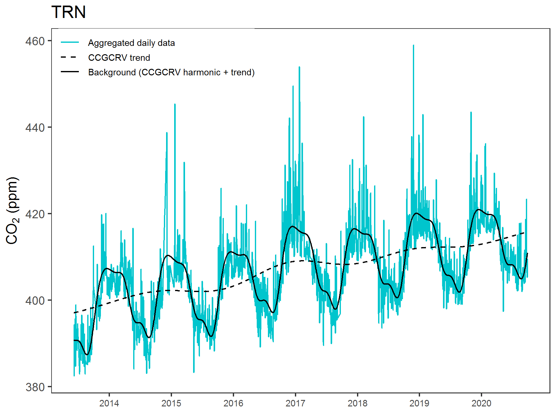
Figure 2The background signal derived at TRN by combining the harmonic component of the CCGCRV function fit to the data and the long-term trend component.
We then extract the smoothed seasonal cycle, S(t), defined as the function C(t) plus the short-term filter of the residuals. We use two different settings for the short-term filter fs, equivalent to 30 and 90 d. We then calculate the difference between S(t) and the harmonic on each day t for both seasonal cycle curves to derive the vectors δC30 and δC90. These are then used to compute variability vectors σ30 and σ90, which are adjusted to reflect seasonal patterns in CO2 and CH4 variability. This adjustment is done by taking the standard deviation of all δC values within a moving window of 90 calendar days around t and 90 d around the same calendar day in all other years in the record. Thus for each calendar day d in a time series consisting of n years,
For example, the σ value for 10 January at TRN would be the standard deviation of the δC values between 26 November 2013 and 24 February 2014, between 26 November 2014 and 24 February 2015, etc., up to 24 February 2020 (or as many of those days exist in the record). The use of this 90 d window is based on the consideration that the amplitude of deviations from the background signal is not uniform throughout the year; variability tends to be higher in the winter months when increased fossil fuel burning and decreased vertical mixing tend to result in high positive signal spikes and during the early spring months when enhanced photosynthesis and increased terrestrial carbon uptake induce large negative peaks. The calculated σ values are thus used to produce envelopes about the background curve representing the range of “normal” or expected variability in the signal, depending on the time of year. In general, this is meant to encapsulate slight interannual fluctuations in the seasonal cycle. Finally, the σ values are multiplied by 2 to further restrict the definition of outlier events. The selection of a ±2σ envelope width represents a compromise between the desire to disregard smaller, site-specific signal excursions (which we term “localized fluctuations”) to the extent possible while retaining the capacity to capture the true magnitudes of atypical regional events. Figure 3 shows the CCGCRV harmonic and the 30 and 90 d smoothed, detrended seasonal cycle of CO2 at TRN for the period 2013–2020.
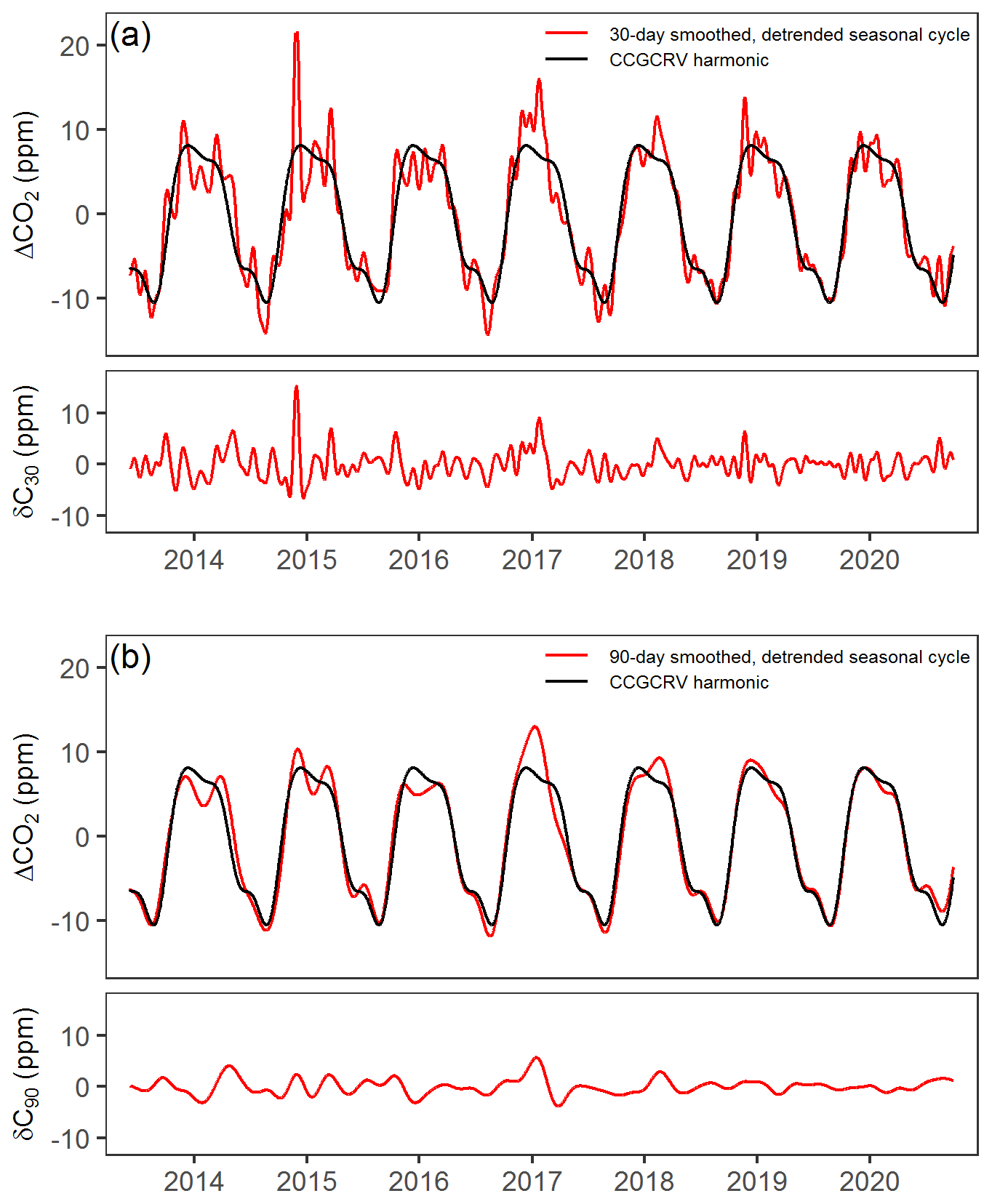
Figure 3The smoothed, detrended seasonal cycle at TRN (red) extracted using (a) 30 and (b) 90 d short-term filters of the CCGCRV function residuals. ΔCO2 represents the calculated mean seasonal variation in CO2, excluding the long-term trend.
The algorithm next smooths the raw data via a LOESS (locally estimated scatterplot smoothing) function (Cleveland, 1979) implemented via the R stats package (R Core Team, 2019). This is done as a way of filtering the daily data and attenuating the influence of short-duration, high-intensity signal spikes when categorizing deviations from the background as anomalies vs. normal signal instabilities. Short-duration (≤ 1 d) spikes are not uncommon in continuous greenhouse gas measurements and are often related to instrument errors or localized perturbations from contaminated air masses. Smoothing the daily data ensures that these short-duration spikes are less heavily weighted and that spikes will only be considered non-background if part of a cluster of other nearby measurements that fall outside the range of expected variability. The LOESS algorithm is applied using a smoothing span (bandwidth) of 30 and 90 d. Anomalous events are then identified by comparing the smoothed daily values to the respective ±2σ range for each day; i.e., the 30 d LOESS curve is compared to the ±2σ30 envelope and the 90 d curve to the ±2σ90 envelope.
The goal of the 30 d analyses is to identify synoptic-scale anomalies (SSAs). We identify these as peaks in the signal where the smoothed daily value is outside the ±2σ envelope for at least 2 consecutive days. We focus these analyses on the extended winter season (November–March) when effects on the signal not directly related to synoptic-scale meteorology – including terrestrial biosphere exchanges – are minimized. We consider 30 d sufficiently wide to mask short (≤ 1 d) spikes yet precise enough to detect the signals of distinct atmospheric transport episodes (as opposed to more generalized effects of seasonal trends in circulation patterns). For example, winter weather in Europe may be influenced at seasonal timescales by the phase and strength of the NAO (e.g., Trigo et al., 2002; Haarsma et al., 2019), which can produce broad signal anomalies in years with consistently developing strong NAO indicators. With a bandwidth of 30 d, these broader patterns should be less apparent, while individual synoptic events such as Scandinavian blocking (BLO) regimes should still leave an identifiable imprint on the signal.
Although we focus primarily on CO2 in the analysis, we also attempt to validate the SSA detection by applying the methodology to concurrent CH4 records from the 10 sites. Emissions of both CH4 and CO2 largely occur over the continents (Friedlingstein et al., 2020; Saunois et al., 2020). Thus, if positive CO2 anomalies during the winter months coincide with periods of sustained transport of easterly winds from the continental interior, such as when NAO conditions or BLO regimes prevail, then they should be more or less synchronized with CH4 spikes. Meanwhile, concentrations of both species should approach background levels when westerly, marine-influenced winds predominate. Although this approach is complicated slightly by the fact that the annual CH4 cycle is less distinct than that of CO2, our envelope is wide enough that measurements must be rather far from the mean annual cycle determined by CCGCRV for several consecutive days in order to register as SSAs. The method should therefore be able to adequately discern anomalous signal components for both species in most winters.
The 90 d analysis is intended for the extraction of longer-term seasonal anomalies. In effect, any period when the 90 d LOESS curve is outside the ±2σ90 envelope is considered to be an anomalous event. At such a wide bandwidth, the smooth curve should be minimally affected by regional signals lasting from a few days to a few weeks, leaving only a broader signal representative of seasonal effects (Ruckstuhl et al., 2012). Anomalies may be induced by enhanced spring carbon uptake; extended droughts; or, to give a more germane example, wide-scale emissions reductions due to global pandemics. For the 90 d application, we concentrate on the extended summer growing season (April–October) to examine the capacities of the methodology in detecting large-scale terrestrial biosphere anomalies. We focus in particular on the summer of 2018, which saw a spate of intense droughts and heat waves across central and northern Europe that altered continent-wide gross primary production (GPP) and CO2 storage and flux patterns (Lindroth et al., 2020; Ramonet et al., 2020; Rinne et al., 2020; Wang et al., 2020).
3.1 SSAs
Table 2 summarizes the results of the SSA extraction for the 10 sites for the period 1 November 2015 to 31 March 2020. This period is selected since the winter of 2015–2016 is the first year in which we have CO2 data available at enough sites to accurately discern the number of localized fluctuations detected at each site, for which we require that CO2 data must be present at no fewer than five sites. Localized fluctuations are defined as SSAs with no analog at any other site, i.e., spikes at a single site which do not coincide with a similar spike elsewhere. These are identified manually after running the algorithm. Figure 4 shows the background CO2 signal, ±2σ envelope (shaded in gray) and 30 d LOESS curve at each of the 10 sites. The period 1 July 2018 to 1 July 2019 is selected as an example. An analogous paneled figure for CH4 is presented as Fig. 5.
Table 2Total number of SSAs in the CO2 signal extracted by the ADA for the period 1 November 2015 to 31 March 2020 based on the ±2σ envelopes defined using the 30 d smoothed seasonal cycle. Localized fluctuations are site-specific events with no analog at any other site (data must be present at a minimum of five sites for comparison).

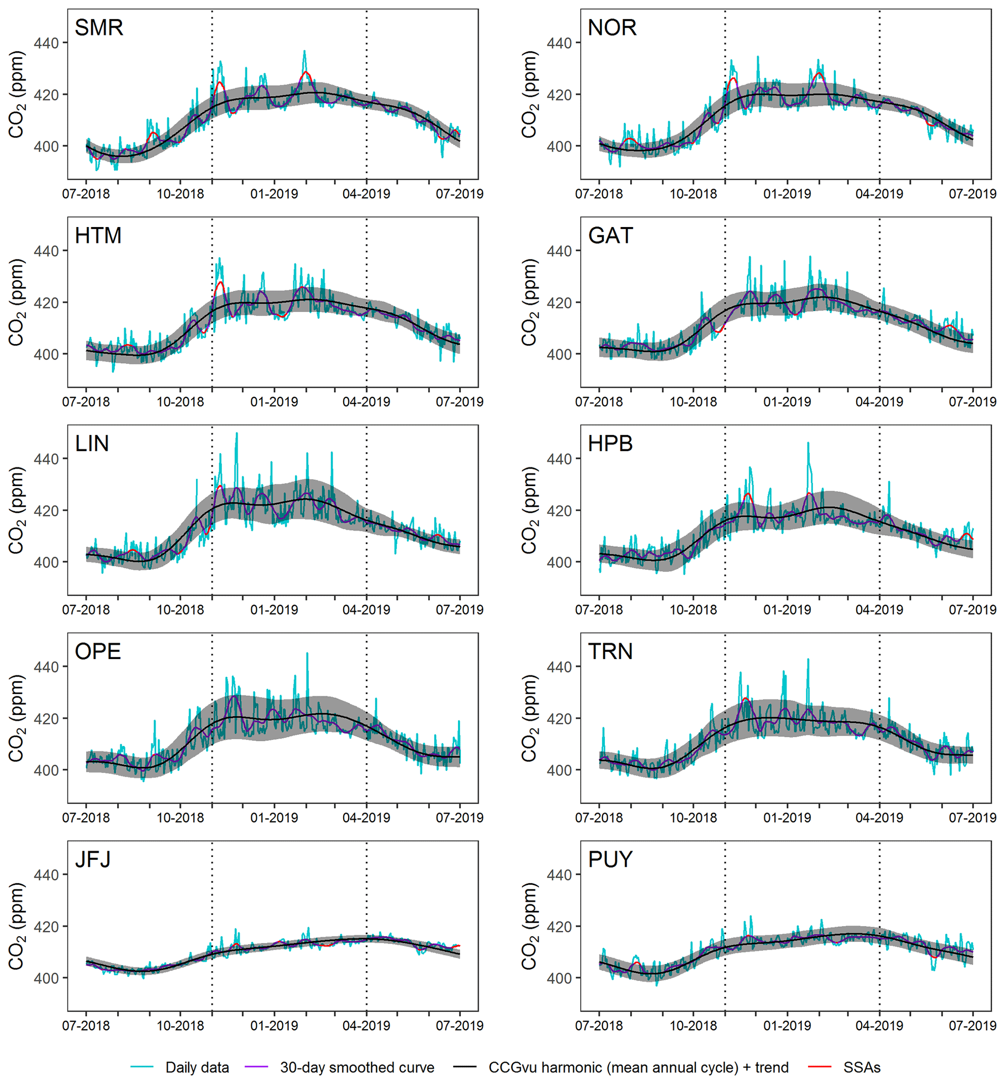
Figure 4Daily aggregated CO2 readings for 1 July 2018–1 July 2019 (blue). The background signal derived using the CCGCRV harmonic + trend curve is shown in black. The gray envelope represents the ±2σ range of the 30 d smoothed cycle about the background signal, and the purple curve is a 30 d smoothing of the daily data. SSAs are highlighted in red. Dashed lines show the extended winter period.
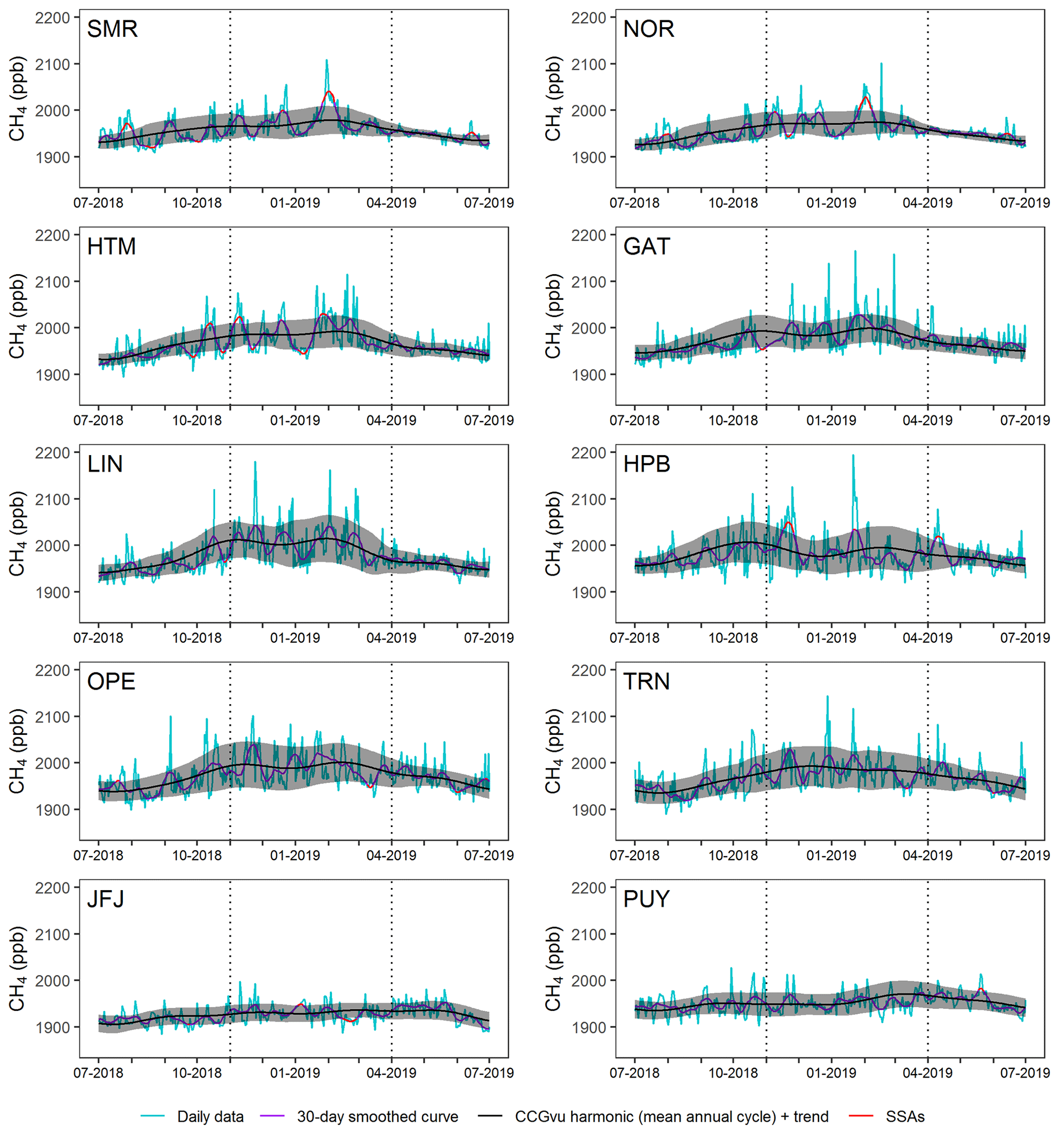
Figure 5Daily aggregated CH4 readings for 1 July 2018–1 July 2019 (blue). The background signal derived using the CCGCRV harmonic + trend curve is shown in black. The gray envelope represents the ±2σ range of the 30 d smoothed cycle about the background signal, and the purple curve is a 30 d smoothing of the daily data. SSAs are highlighted in red. Dashed lines show the extended winter period.
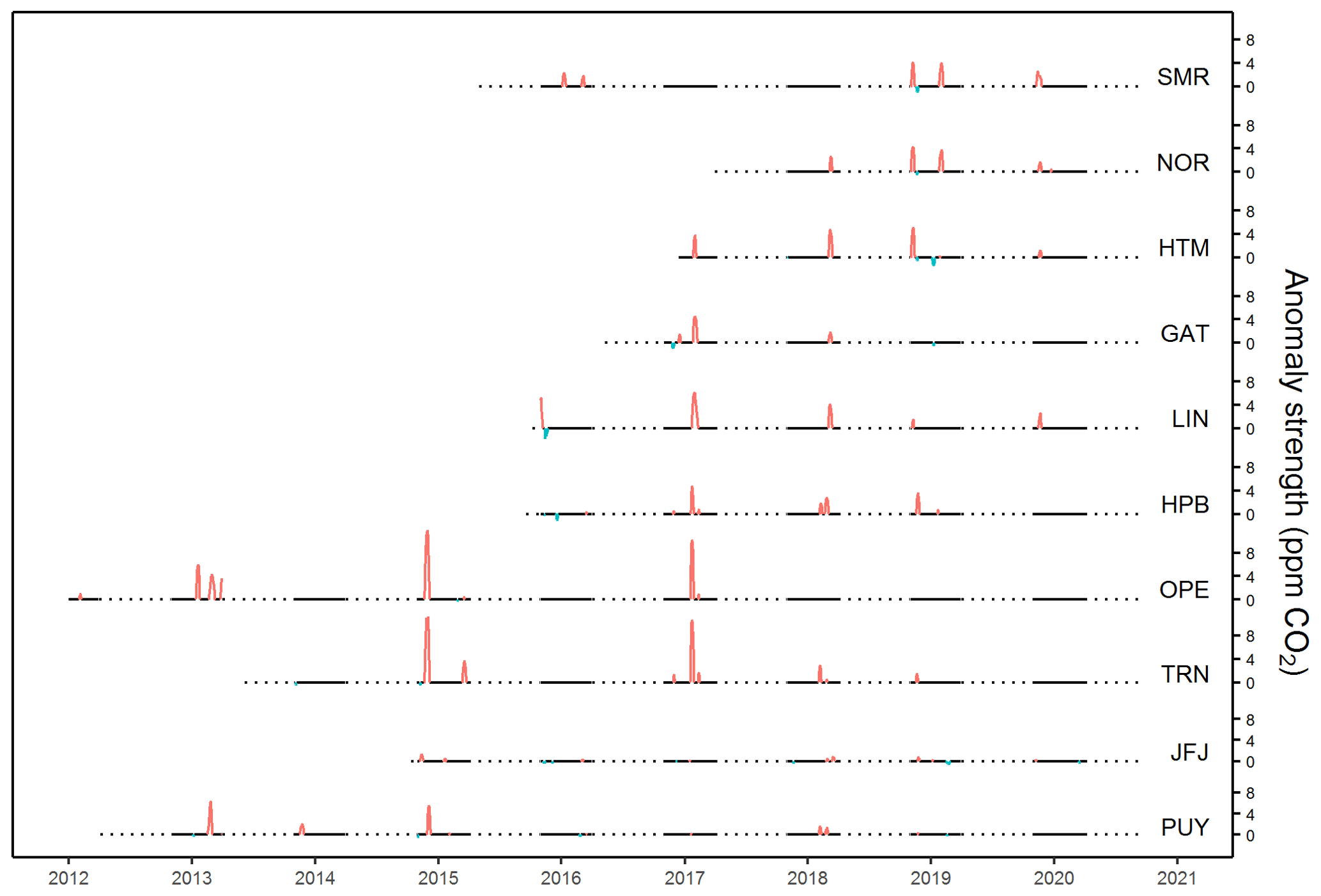
Figure 6Positive (red) and negative (blue) SSAs in the complete CO2 records of each site. The anomaly strength refers to the difference between the 30 d LOESS curve and the boundary of the ±2σ30 envelope.
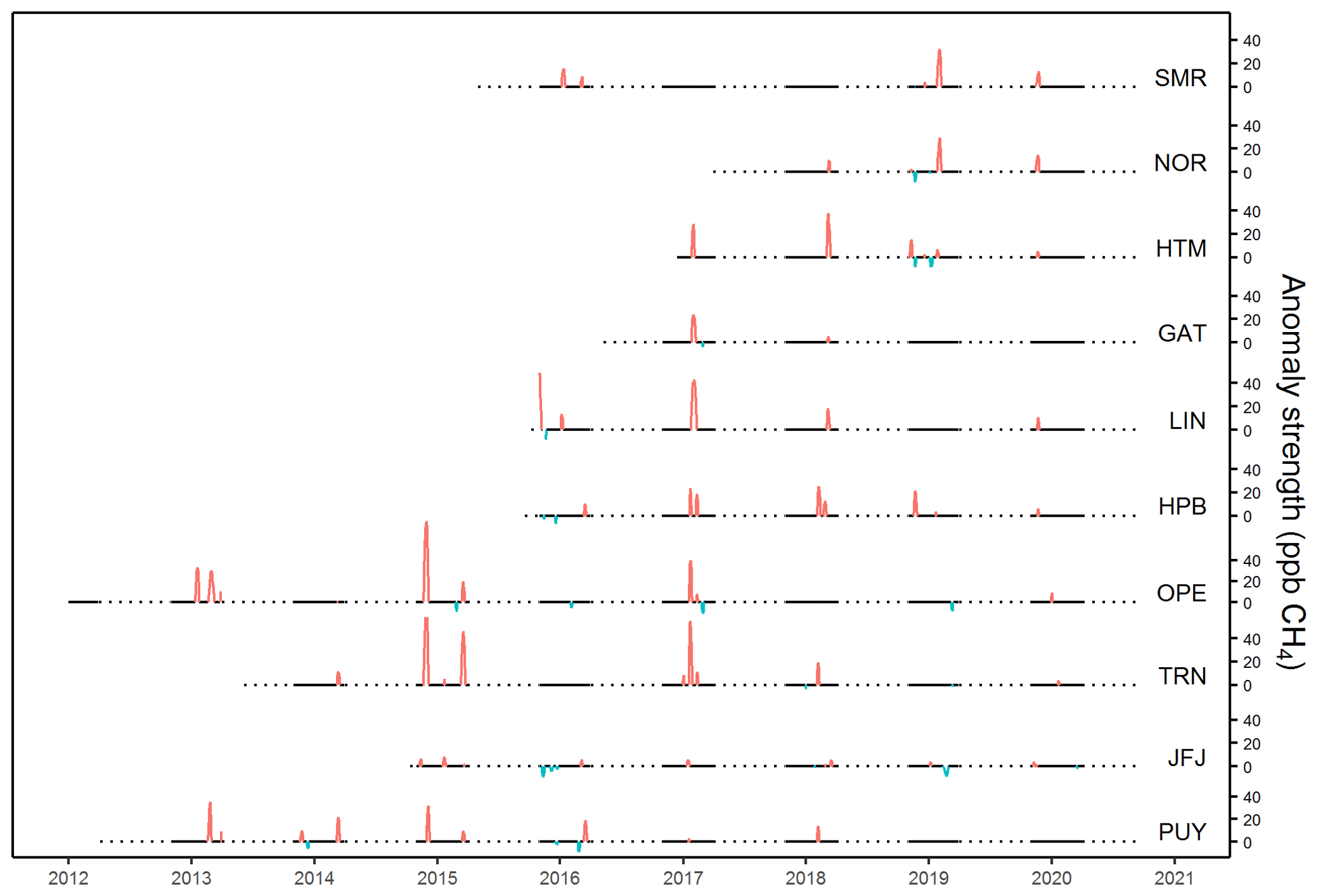
Figures 6 and 7 show the difference between the LOESS curves and the envelope boundaries for measurements outside of the ±2σ range for CO2 and CH4, respectively. Positive SSAs (above the envelope) are shown in red, while negative SSAs are shown in blue. Periods where measurements fall within the envelope are represented by flat, black lines. Note that only winter periods (November–March) are shown.
Overall, the algorithm produces similar patterns for both CO2 and CH4 at the three Scandinavian sites (SMR, NOR, HTM). In particular, the ADA seems to identify simultaneous positive CO2 anomalies in November 2018, January/February 2019 and November 2019 at SMR, NOR and HTM. These three northernmost sites also share some similarities with the three German sites (GAT, LIN, HPB); both the November 2018 spike and the early 2019 spike are captured at HPB for both trace gases, while the November 2018 spike is captured at LIN for CO2. Regarding the CH4 records, the same November 2018 spike is captured at HTM and HPB, while a similar early 2019 CO2 spike is seen at SMR, NOR, HTM and HPB. Smaller synchronic positive CO2 anomalies with broader geographic extents are seen in January 2017 (at HTM, GAT, LIN, HPB, OPE and TRN) and March 2018 (at NOR, HTM, GAT, LIN, HPB, TRN and PUY). In both cases, these continent-wide anomalies are well synchronized with the CH4 patterns, which show spikes with similar timing at nearly all of the same stations. For the southernmost sites, for which records date back prior to the winter of 2015–2016, several simultaneous anomalies are observed, including one in February/March 2013 (OPE, PUY), and an especially large signal excursion seen at the three French sites (OPE, TRN and PUY) in November/December 2014. Both of these coincide with CH4 events of comparable magnitude.
3.2 Seasonal anomalies
Figure 8 shows the 90 d extraction procedure at each of the 10 sites and is analogous to Fig. 4, except that we show the period 1 January 2018 to 1 January 2019 as we wish to assess the algorithm's performance with regard to the timing, intensity and extent of the 2018 drought and heat wave events across central and northern Europe (Ramonet et al., 2020). Figure 9 shows the anomaly patterns at the 10 sites during the extended growing season (April–October). For reference, we also include the average April–October standardized precipitation evapotranspiration index (SPEI; Vicente-Serrano et al., 2010) values at each site location to represent the relative intensity of drought conditions throughout the summer.
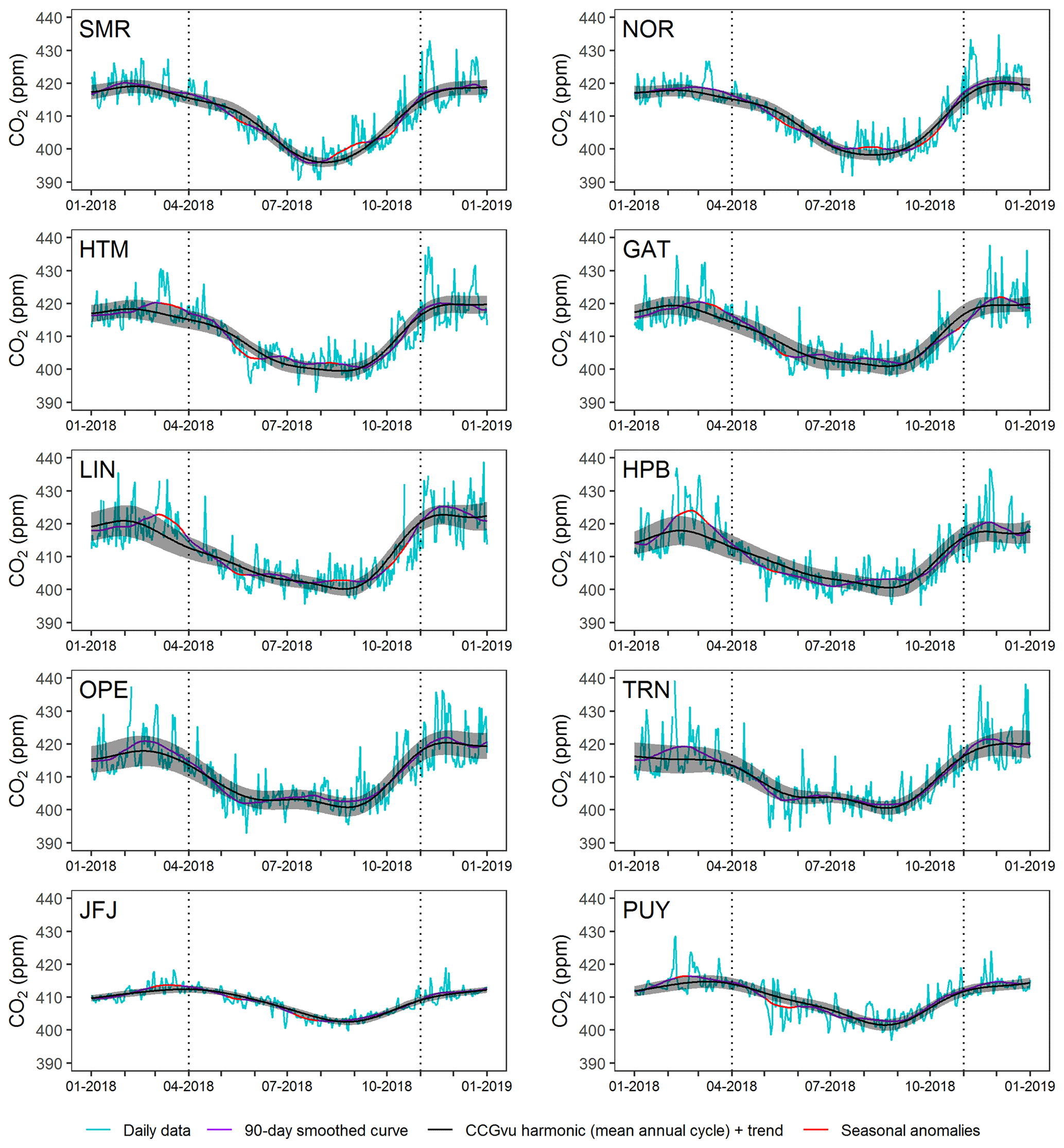
Figure 8Daily aggregated CO2 readings for 1 January 2018–1 January 2019 (blue). The background signal derived using the CCGCRV harmonic + trend curve is shown in black. The gray envelope represents the ±2σ range of the 90 d smoothed cycle about the background signal, and the purple curve is a 90 d smoothing of the daily data. Anomalous periods are highlighted in red. Dashed lines delineate the growing season (April–October).
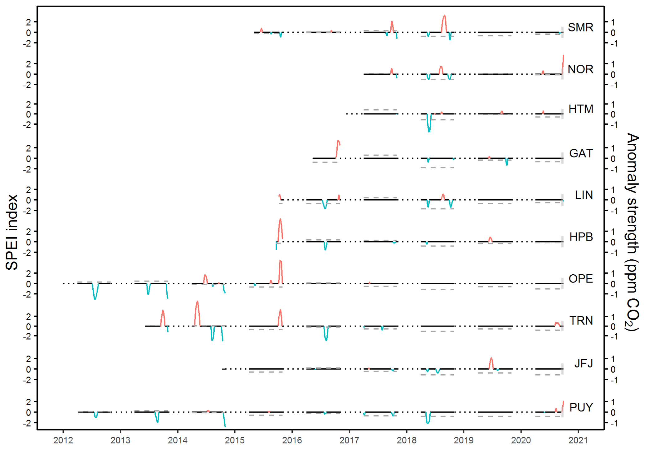
Figure 9Positive (red) and negative (blue) 90 d seasonal CO2 anomalies. April–October average SPEI values are indicated by the dashed gray lines. The gray bar on the right end of the plots indicates the standard deviation of summer SPEI values from 1999–2020.
The CO2 patterns observed during the growing season of 2018 are consistent with the timing of terrestrial biospheric aberrations that characterized that year's exceptional drought conditions. The ADA finds negative CO2 anomalies in May 2018 at all sites except for OPE and TRN. The largest of these is at HTM, although a fairly large spike is detected at PUY as well. This may be a product of unusually warm and sunny early spring conditions in 2018, which contributed to early green-up and growth across the region and led to enhanced net biome production (NBP) and plant CO2 uptake. Subsequent extreme heat and dry conditions led to a lapse in summertime productivity and reduced photosynthesis (Ramonet et al., 2020), which may explain the July CO2 spikes captured at SMR, NOR, HTM and LIN. The ensuing dip in CO2 observed at SMR, NOR and LIN in September 2018 can plausibly be interpreted as a legacy effect of the reduced summertime productivity; drought stress likely led to decreased litter availability in the fall and hence lower-than-normal decomposition rates and total ecosystem respiration (Bastos et al., 2020).
Several other multi-site anomalies are captured at the three French sites in the summers of 2012–2015, though the lack of recordings at the other sites makes it unclear whether these represent smaller-scale meteorological occurrences or broader regional patterns. We note, however, that the large positive spike seen at OPE and TRN in October 2015 followed an intense summer dry spell that year (Erdman, 2015). This could plausibly have triggered early senescence onset and reduced photosynthetic activity in the fall. Likewise, an unusually wet summer in France in 2014 might have led to increased ecosystem productivity in the fall, resulting in the negative spike seen simultaneously at OPE, TRN and PUY in that year. We note also that in general, at OPE and TRN, anomalous enhanced maximum CO2 uptake (indicated by negative spikes in early to mid-summer) appears to correlate with higher SPEI values (wetter conditions).
Worth noting is that although some summertime anomalies detected at the 90 d bandwidth correlate with known periods of exceptional enhancement or suppression of biospheric productivity, we have not attempted to establish a causal link between the two here. This would require a detailed quantification of the direct impacts of atmospheric transport. In the summer of 2018, for example, the positive CO2 anomaly we observe across several sites agrees well with estimated reductions in continent-wide photosynthesis predicted by flux inversion studies (e.g., Ramonet et al., 2020). However, the timing of this anomaly also corresponds with the presence of a high-pressure blocking system which formed over the region in June and July 2018, which may have enhanced easterly CO2 transport through persistent anticyclone formation (Rösner et al., 2019). The extent to which this may have been the case is not examined in detail. Similar spikes, alluded to above, which appear to track known meteorological events of exceptional duration and/or intensity likewise cannot be said to exclusively reflect NPP irregularities without the additional implementation of back-trajectory or wind sector analyses. Such an analysis is outside the scope of this report, which tends more toward a technical description of our algorithm and its potential applications than a detailed climatological study.
Several potential challenges may arise in the technical application of the ADA. These include the presence of large data gaps in time series which could arise from instrument malfunctions or other technical issues. CCGCRV is ill-suited to handle such gaps (Pickers and Manning, 2015), meaning missing data points must be artificially imputed using a structural modeling function or linearly interpolated. We opt for the latter by applying the method of Moritz and Bartz-Beielstein (2017), which is sufficient for small data gaps but generally impractical for large ones (∼ 1 month), where simple linear interpolation can potentially result in erroneous anomaly selection. This appears to be the case, for example, in late October 2018 at GAT, where the algorithm detects negative anomalies in both trace species coinciding with the start of a month-long gap in the daily readings (Figs. 4 and 5). Significant data gaps such as this should thus be identified before performing the linear interpolation and applying the anomaly extraction so that any quantification of the signal during these periods is regarded with caution. One potential workaround is to interpolate data gaps using the values of the multi-year average detrended seasonal cycle at a site. This has not been attempted here since it would require an a priori interpolation of data gaps, i.e., via a linear interpolation, followed by an a posteriori re-interpolation of the same gaps, followed by a secondary application of the CCGCRV fitting procedure. It is unclear whether any reduction in gap-related false positive detection, which appears to be quite rare overall, justifies such a trade-off in efficiency.
The reliability of the results may also be strongly influenced by the range of available data. Sites with longer historical records will have a larger residual dataset to draw from, allowing for more precision when extracting the mean annual cycle and resultant ±2σ envelope, while sites with shorter records may produce less precise results. The potential drawbacks of this are twofold; (1) very slight anomalies might tend to be obscured at sites with a limited number (∼ 3–4 years) of relatively capricious measurements, and (2) low-amplitude localized fluctuations might be detected at sites where the full range of expected seasonal variability is underestimated by the ±2σ envelope, or the background curve is an imprecise fit to the true seasonal cycle. Anomaly patterns at sites with shorter records should thus be regarded with caution and cross-validated with patterns from other nearby sites if possible. In the future, as longer historical records become available at a greater number of ICOS stations, a standardized setting for the record length used to estimate the background (e.g., 10 years) may be adopted.
Furthermore, the method may have limited applicability at more isolated sites that have no clear analog within the ICOS network. Evaluation of anomalies through cross-validation is difficult if a site has relatively few nearby sister stations which can reasonably be expected to sample from similar air masses most of the time. This drawback is apparent when considering the results at PUY and JFJ, both background sites which sample frequently from well-mixed air above the planetary boundary layer (Asmi et al., 2011; Herrmann et al., 2015). At PUY, for example, planetary boundary layer (PBL) height analyses reveal that the station samples from the free troposphere more than 70 % of the time and up to 81 % in the winter (Lopez et al., 2015). With such infrequent sampling of surface air, air parcels most likely to contain the carbon signatures of bellwether biospheric events (such as droughts and their legacy effects) or shorter-term anomalies linked to localized contaminant plumes or sudden changes in atmospheric transport patterns may go undetected. At JFJ, PBL air is sampled only intermittently when conditions favor mountain venting or advection (Zellweger et al., 2003; Griffiths et al., 2014), meaning short-duration anomalies may merely reflect the prevalence of such localized phenomena rather than broader atmospheric transport patterns. In the future, this limitation will become less important as the ICOS Atmosphere network continues to grow in size; 26 stations across Europe currently possess the ICOS label, and another dozen or so are set to join soon.
The occasional selection of localized fluctuations is an additional concern. In some cases, low-amplitude spikes classified as anomalies at a particular station might not truly represent significant regional-scale excursions from the background signal. This implies the need for station-specific protocols to classify anomalies based on duration and magnitude, which may require cross-validation using multiple station readings or manual inspection by principal investigators. The similarity in the patterns at the six northernmost sites, for example, offers a means of validation for the detection of SSAs; since true synoptic-scale anomalies should produce a signal over a broad swath of the continent, those anomalies observed only at certain sites can reasonably be assumed to indicate localized events. Note, for example, the very slight positive anomaly in December 2016 seen only at GAT (Fig. 6).
In other cases, signal excursions might register as anomalies at certain sites but not others. In such cases, users may determine that these events are noteworthy enough that they should be classified as anomalies more broadly. The recourse then is a site-specific refinement of the selection criteria or tuning of the algorithmic parameters. For example, although we use a bandwidth of 30 d for SSA detection, this choice may not be the most appropriate in all cases. Different stations have different ambient signal variability ranges depending on their geographical setting and proximity to emission sources; those with higher overall variability (and hence wider ±2σ ranges) might record too few SSAs if applying an excessively wide smoothing span as peaks in the smoothed signal would be dampened sufficiently to be contained within the envelope. Users may thus find a bandwidth of, for example, 15–25 d to produce more informative results at some locations. Likewise, sites with lower overall variability might tend to record too many SSAs when using a bandwidth that is too short. By definition, the envelope width also affects the anomaly selection. Note, for example, that the 2018 drought pattern typified at the six northernmost sites does not appear at OPE or TRN in Fig. 9. A closer examination of Fig. 8 reveals that while measurements at these two sites during, for example, May 2018 were below the mean annual cycle, no anomalous springtime CO2 dip was registered since the smooth curves at OPE and TRN were still contained within the ±2σ envelope bounds. As mentioned, the specification of a ±2σ threshold stems from our desire to avoid excessive selection of low-amplitude, site-specific signal peaks. However, this width might mask noteworthy seasonal patterns at certain sites with greater year-round variability, making cross-examination all the more critical.
Uncertainties can also arise in the interpretation of the results. For example, the distinction we make between synoptic-scale and seasonal anomalies is primarily based on the length of observed signal spikes. Normally, SSAs which persist from 1–2 d to several weeks are presumed to be linked to prevailing wind conditions at a given site and hence changes in the source regions of sampled air parcels, e.g., from relatively clean North Atlantic air to continental-sourced air parcels bearing the signatures of terrestrial emissions. However, in some cases, anomalies deemed to be seasonal in length may simply represent the frequent occurrence or unusual persistence of synoptic-scale atmospheric transport patterns. For example, as alluded to previously, the extreme heat waves in northern and central Europe throughout much of June and July 2018 were associated with the persistence of a high-pressure blocking system which formed over the region. Although synoptic in size, this pressure anomaly – combined with high temperatures – had resounding effects on European forests and resulted in subsequent CO2 anomalies in the fall of 2018. It is thus more appropriately considered to be part of a broader seasonal anomaly. The implication is that in some cases, “seasonal” anomalies are rather patterns which consist of a series of shorter, related signal irregularities. These irregularities will often be visible at shorter bandwidths and could be directly linked to meteorological events. Summertime anomalies should thus be considered in the wider context of terrestrial ecosystem production, indicators of which may lag well behind the occurrence of exceptional transport episodes.
In general, we find that the algorithm captures well the signature effects of unusually strong or persistent atmospheric transport regimes in the wintertime. This interpretation is reinforced by the fact that the CO2 and CH4 anomaly patterns during the extended winter season are strikingly similar for the 30 d implementation of the methodology. The ADA also shows promising potential with regard to detecting the imprints of regional and continent-wide extremes in NBP and other ecosystem indicators, specifically the distinctive markings of the 2018 European drought, on which we have placed particular emphasis. An analysis of the effects of summertime atmospheric transport is required to more definitively score the method's capacity to correctly identify exceptional biospheric episodes.
The robustness of the results is reliant on cross-validation of anomaly detection across multiple sites. However, we note that anomalies of sufficient size – e.g., ∼ 3 ppm CO2 greater than our ±2σ envelope boundary when using a 30 d bandwidth or ∼ 0.5 ppm CO2 when using a 90 d bandwidth – will usually register simultaneously at multiple sites within the same region and seem generally unlikely to stem from localized contamination. The method also has a low computational cost, and the process of including additional sites in an analysis is relatively straightforward. As new NRT (level 1) GHG data are uploaded to the ICOS CP, users have only to concatenate these to existing datasets and reinitiate the method beginning with the steps outlined in Sect. 2.3. A fully automated Python implementation of the code is available online in which L2 and L1 data for a given station are extracted directly from the ICOS CP and concatenated to form a continuous multi-year time series for all dates up to the present. Users also have the option to extract longer historical records than those available through the ICOS CP and preprocess these themselves before running the code. The current default implementation is to produce time series plots in the style of Figs. 6, 7 and 9.
The ability to detect in NRT the occurrence of non-background signal events at multiple timescales is central to an improved understanding of GHG variability and regional carbon cycling processes at multiple timescales, and the ADA represents an important step toward this end. Eventually, our aim is to make results available online so that station managers and other end users can be alerted in NRT when anomalous signal events occur, i.e., through the automated generation of data files and time series plots to display on the sites' respective panel board pages.
The ADA is intended to be open-source, and the R code is currently accessible via a GitHub repository page (https://github.com/hellonskis/ICOS_ATC_anomaly_detection) (DOI: https://doi.org/10.5281/zenodo.4639780, Resovsky, 2021a). Python code is available internally via the ICOS Jupyter hub at https://jupyter3.icos-cp.eu/ (last access: 16 April 2021) and is available upon request. An open-source version of the Jupyter code is also available online at https://doi.org/10.5281/zenodo.5166711 (Resovsky, 2021b).
The ADA is developed at the ICOS ATC (LSCE) in Gif-sur-Yvette, France. The code is intended to be applied to datasets consisting of validated (level 2) hourly values and NRT (level 1) measurements. Level 2 data are available online (https://doi.org/10.18160.WJY7-5D06; ICOS Research Infrastructure, 2021). Level 1 data are available online (https://doi.org/10.18160.ATM_NRT_CO2_CH4; ICOS Research Infrastructure, 2018).
All code required to run the ADA was written and is maintained by AR. AR carried out all experiments and produced the figures and text in this paper. MR manages the OPE and PUY stations and also contributed the conceptual idea behind the ADA as well as many hours of advice and feedback, especially on the sections discussing the 2018 European drought. LR was instrumental in finalizing the layout of the figures and the experimental workflow detailed in the methodology section. JT assisted in pre-processing of ICOS data products and provided scientific advice regarding the smoothing procedures used to extract anomalies. PC provided suggestions related to the terminology used for the text and figures, descriptions of the 2018 European drought and its aftereffects, and additional data analysis considerations included in the discussion section. MS is the manager of the JFJ station data and also provided a great deal of advice and feedback regarding the organization of this paper and the presentation of the ideas herein. MH (HTM), DK, ML, JMW (GAT, HPB, LIN), IM (SMR), MM (NOR) and SC (OPE) are the station managers for the seven other stations whose data are used in this paper. RE is the deputy head of the Copernicus Atmosphere Monitoring Service, whose contributions made this work possible.
The authors declare that they have no conflict of interest.
Publisher’s note: Copernicus Publications remains neutral with regard to jurisdictional claims in published maps and institutional affiliations.
This work was made possible by the Copernicus Atmosphere Monitoring Service (CAMS), which is funded under regulation no.377/2014 of the European Parliament and of the Council of 3 April 2014 establishing the Copernicus program (“the Copernicus Regulation”) and operated by the ECMWF under an agreement with the European Commission dated 11 November 2014 (“ECMWF Agreement”). The authors also acknowledge the persons in charge of the 10 monitoring stations, which are part of the ICOS Atmosphere network. ICOS Atmosphere stations are supported through national consortia and funding agencies. JFJ observations are supported through ICOS Switzerland, which is funded by the Swiss National Science Foundation (grants 20FI21_148992 and 20FI20_173691) and in-house contributions. GAT, HPB and LIN observations are supported through ICOS Germany and funded by the German Ministry of Transport and Digital Infrastructure (DWD) and in-house contributions. OPE, PUY and TRN are supported through ICOS France, ANDRA, CEA and CNRS. HTM and NOR are supported by ICOS Sweden and Lund University. SMR is supported by ICOS Finland and the University of Helsinki. We also wish to thank all members of the ICOS Atmosphere Monitoring Station Assembly for their contributions to the discussions surrounding anomalous signal detection techniques.
This research has been supported by the Commissariat à l'énergie atomique et aux énergies alternatives (CEA) (grant no. ECMWF/Copernicus/2016/CAMS_26).
This paper was edited by Can Li and reviewed by two anonymous referees.
Apadula, F., Cassardo, C., Ferrarese, S., Heltai, D., and Lanza, A.: Thirty Years of Atmospheric CO2 Observations at the Plateau Rosa Station, Italy, Atmosphere, 10, 418, https://doi.org/10.3390/atmos10070418, 2019.
Asmi, A., Wiedensohler, A., Laj, P., Fjaeraa, A.-M., Sellegri, K., Birmili, W., Weingartner, E., Baltensperger, U., Zdimal, V., Zikova, N., Putaud, J.-P., Marinoni, A., Tunved, P., Hansson, H.-C., Fiebig, M., Kivekäs, N., Lihavainen, H., Asmi, E., Ulevicius, V., Aalto, P. P., Swietlicki, E., Kristensson, A., Mihalopoulos, N., Kalivitis, N., Kalapov, I., Kiss, G., de Leeuw, G., Henzing, B., Harrison, R. M., Beddows, D., O'Dowd, C., Jennings, S. G., Flentje, H., Weinhold, K., Meinhardt, F., Ries, L., and Kulmala, M.: Number size distributions and seasonality of submicron particles in Europe 2008–2009, Atmos. Chem. Phys., 11, 5505–5538, https://doi.org/10.5194/acp-11-5505-2011, 2011.
Balzani Loöv, J. M., Henne, S., Legreid, G., Staehelin, J., Reimann, S., Prévôt, A. S. H., Steinbacher, M., and Vollmer, M. K.: Estimation of background concentrations of trace gases at the Swiss Alpine site Jungfraujoch (3580 m a.s.l.), J. Geophys. Res., 113, D22305, https://doi.org/10.1029/2007JD009751, 2008.
Bastos, A., Ciais, P., Friedlingstein, P., Sitch, S., Pongratz, J., Fan, L., Wigneron, J. P., Weber, U., Reichstein, M., Fu, Z., Anthoni, P., Arneth, A., Haverd, V., Jain, A. K., Joetzjer, E., Knauer, J., Lienert, S., Loughran, T., McGuire, P. C., Tian, H., Viovy, N., and Zaehle, S.: Direct and seasonal legacy effects of the 2018 heat wave and drought on European ecosystem productivity, Sci. Adv., 6, eaba2724, https://doi.org/10.1126/sciadv.aba2724, 2020.
Biraud, S., Ciais, P., Ramonet, M., Simmonds, P., Kazan, V., Monfray, P., O'Doherty, S., Spain, T. G., and Jennings, S. G.: European greenhouse gas emissions estimated from continuous atmospheric measurements and radon 222 at Mace Head, Ireland, J. Geophys. Res., 105, 1351–1366, https://doi.org/10.1029/1999JD900821, 2000.
Bladé, I., Liebmann, B., Fortuny, D., and van Oldenborgh, G. J.: Observed and simulated impacts of the summer NAO in Europe: implications for projected drying in the Mediterranean region, Clim. Dynam., 39, 709–727, https://doi.org/10.1007/s00382-011-1195-x, 2011.
Chambers, S., Williams, A., Conen, F., Griffiths, A., Reimann, S., Steinbacher, M., Krummel, P. Steele, L., Van der Schoot, M., Galbally, I., Molloy, S., and Barnes, J. F.: Towards a Universal “Baseline” Characterization of Air Masses for High- and Low-Altitude Observing Stations Using Radon-222, Aerosol Air Qual. Res., 16, 885–899, https://doi.org/10.4209/aaqr.2015.06.0391, 2016.
Cleveland, W. S.: Robust Locally Weighted Regression and Smoothing Scatterplots, J. Am. Stat. Assoc., 74, 829–836, https://doi.org/10.1080/01621459.1979.10481038, 1979.
Cui, J., S., Pandey Deolal, S., Sprenger, M., Henne, S., Staehelin, J., Steinbacher, M., and Nédélec, P.: Free tropospheric ozone changes over Europe as observed at Jungfraujoch (1990–2008): An analysis based on backward trajectories, J. Geophys. Res., 116, D10304, https://doi.org/10.1029/2010JD015154, 2011.
El Yazidi, A., Ramonet, M., Ciais, P., Broquet, G., Pison, I., Abbaris, A., Brunner, D., Conil, S., Delmotte, M., Gheusi, F., Guerin, F., Hazan, L., Kachroudi, N., Kouvarakis, G., Mihalopoulos, N., Rivier, L., and Serça, D.: Identification of spikes associated with local sources in continuous time series of atmospheric CO, CO2 and CH4, Atmos. Meas. Tech., 11, 1599–1614, https://doi.org/10.5194/amt-11-1599-2018, 2018.
Erdman, J.: Heat Records Shattered in Germany, France, The Netherlands in June/July 2015 Europe Heat Wave, The Weather Channel, available at: https://weather.com/forecast/news/europe-heat-wave-record-highs-june-july-2015 (last access: 2 December 2020), 8 July 2015.
Friedlingstein, P., O'Sullivan, M., Jones, M. W., Andrew, R. M., Hauck, J., Olsen, A., Peters, G. P., Peters, W., Pongratz, J., Sitch, S., Le Quéré, C., Canadell, J. G., Ciais, P., Jackson, R. B., Alin, S., Aragão, L. E. O. C., Arneth, A., Arora, V., Bates, N. R., Becker, M., Benoit-Cattin, A., Bittig, H. C., Bopp, L., Bultan, S., Chandra, N., Chevallier, F., Chini, L. P., Evans, W., Florentie, L., Forster, P. M., Gasser, T., Gehlen, M., Gilfillan, D., Gkritzalis, T., Gregor, L., Gruber, N., Harris, I., Hartung, K., Haverd, V., Houghton, R. A., Ilyina, T., Jain, A. K., Joetzjer, E., Kadono, K., Kato, E., Kitidis, V., Korsbakken, J. I., Landschützer, P., Lefèvre, N., Lenton, A., Lienert, S., Liu, Z., Lombardozzi, D., Marland, G., Metzl, N., Munro, D. R., Nabel, J. E. M. S., Nakaoka, S.-I., Niwa, Y., O'Brien, K., Ono, T., Palmer, P. I., Pierrot, D., Poulter, B., Resplandy, L., Robertson, E., Rödenbeck, C., Schwinger, J., Séférian, R., Skjelvan, I., Smith, A. J. P., Sutton, A. J., Tanhua, T., Tans, P. P., Tian, H., Tilbrook, B., van der Werf, G., Vuichard, N., Walker, A. P., Wanninkhof, R., Watson, A. J., Willis, D., Wiltshire, A. J., Yuan, W., Yue, X., and Zaehle, S.: Global Carbon Budget 2020, Earth Syst. Sci. Data, 12, 3269–3340, https://doi.org/10.5194/essd-12-3269-2020, 2020.
Giostra, U., Furlani, F., Arduini, J., Cava, D., Manning, A. J., O'Doherty, S. J., Reimann, S., and Maione, M.: The determination of a “regional” atmospheric background mixing ratio for anthropogenic greenhouse gases: A comparison of two independent methods, Atmos. Environ., 45, 7396–7405, https://doi.org/10.1016/j.atmosenv.2011.06.076, 2011.
Global Monitoring Laboratory: ccgcrv, NOAA [code], available at: https://gml.noaa.gov/aftp/pub/john/ccgcrv/, last access: 24 June 2021.
Griffiths, A. D., Conen, F., Weingartner, E., Zimmermann, L., Chambers, S. D., Williams, A. G., and Steinbacher, M.: Surface-to-mountaintop transport characterised by radon observations at the Jungfraujoch, Atmos. Chem. Phys., 14, 12763–12779, https://doi.org/10.5194/acp-14-12763-2014, 2014.
Haarsma, R. J., García-Serrano, J., Prodhomme, C., Omar Bellprat, O., Davini, P., and Drijfhout, S.: Sensitivity of winter North Atlantic-European climate to resolved atmosphere and ocean dynamics, Sci. Rep., 9, 13358, https://doi.org/10.1038/s41598-019-49865-9, 2019.
Herrmann E., Weingartner, E., Henne, S., Vuilleumier, L., Bukowiecki, N., Steinbacher, M., Conen, F., Collaud Coen, M., Hammer, E., Jurányi, Z., Baltensperger, U., and Gysel, M.: Analysis of long-term aerosol size distribution data from Jungfraujoch with emphasis on free tropospheric conditions, cloud influence, and air mass transport, J. Geophys. Res., 120, 9459–9480, https://doi.org/10.1002/2015JD023660, 2015.
ICOS Research Infrastructure: ICOS Near Real-Time (Level 1) Atmospheric Greenhouse Gas Mole Fractions of CO2, CO and CH4, growing time series starting from latest Level 2 release (Version 1.0), ICOS ERIC [data set], https://doi.org/10.18160.ATM_NRT_CO2_CH4, 2018.
ICOS Research Infrastructure: ICOS Handbook 2020, 152 pp., ISBN 978-952-69501-1-2, available at: https://www.icos-cp.eu/sites/default/files/cmis/ICOS Handbook 2020.pdf (last access: 8 September 2020), 2020a.
ICOS Research Infrastructure: ICOS Atmosphere Release 2020-1 of Level 2 Greenhouse Gas Mole Fractions of CO2, CH4, CO, meteorology and 14CO2 (1.0), ICOS ERIC – Carbon Portal, https://doi.org/10.18160/H522-A9S0, 2020b.
ICOS Research Infrastructure: ICOS Atmosphere Release 2021-1 of Level 2 Greenhouse Gas Mole Fractions of CO2, CH4, N2O, CO, meteorology and 14CO2 (1.0), ICOS ERIC – Carbon Portal [data set], https://doi.org/10.18160/WJY7-5D06, 2021.
IUPAC: Compendium of Chemical Terminology, 2nd edn. (the “Gold Book”), compiled by: McNaught, A. D. and Wilkinson, A., Blackwell Scientific Publications, Oxford, UK, online version (2019–) created by: Chalk, S. J., https://doi.org/10.1351/goldbook, 1997.
Lindroth, A., Holst, J., Linderson, M.-L., Aurela, M., Biermann, T., Heliasz, M., Chi, J., Ibrom, A., Kolari, P., Klemedtsson, L., Krasnova, A., Laurila, T., Lehner, I., Lohila, A., Mammarella, I., Mölder, M., Löfvenius, M. O., Peichl, M., Pilegaard, K., Soosar, K., Vesala, T., Vestin, P., Weslien, P., and Nilsson, M.: Effects pf drought and meteorological forcing on carbon and water fluxes in Nordic forests during the dry summer of 2018, Phil. Trans. R. Soc. B, 375, 20190516, https://doi.org/10.1098/rstb.2019.0516, 2020.
Lopez, M., Schmidt, M., Ramonet, M., Bonne, J.-L., Colomb, A., Kazan, V., Laj, P., and Pichon, J.-M.: Three years of semicontinuous greenhouse gas measurements at the Puy de Dôme station (central France), Atmos. Meas. Tech., 8, 3941–3958, https://doi.org/10.5194/amt-8-3941-2015, 2015.
Morgan, E. J., Lavrič, J. V., Seifert, T., Chicoine, T., Day, A., Gomez, J., Logan, R., Sack, J., Shuuya, T., Uushona, E. G., Vincent, K., Schultz, U., Brunke, E.-G., Labuschagne, C., Thompson, R. L., Schmidt, S., Manning, A. C., and Heimann, M.: Continuous measurements of greenhouse gases and atmospheric oxygen at the Namib Desert Atmospheric Observatory, Atmos. Meas. Tech., 8, 2233–2250, https://doi.org/10.5194/amt-8-2233-2015, 2015.
Moritz, S. and Bartz-Beielstein, T.: imputeTS: Time Series Missing Value Imputation in R, R J., 9, 207–218, https://doi.org/10.32614/RJ-2017-009, 2017.
O'Doherty, S., Simmonds, P. G., Cunnold, D. M., Wang, H. J., Sturrock, G. A., Fraser, P. J., Ryall, D., Derwent, R. G., Weiss, R. F., Salameh, P., Miller, B. R., and Prinn, R. G.: In situ chloroform measurements at Advanced Global Atmospheric Gases Experiment atmospheric research stations from 1994 to 1998, J. Geophys. Res., 106, 20429–20444, https://doi.org/10.1029/2000JD900792, 2001.
Pal, S., Lopez, M., Schmidt, M., Ramonet, M., Gibert, F., Xueref-Remy, I., and Ciais, P.: Investigation of the atmospheric boundary layer depth variability and its impact on the 222Rn concentration at a rural site in France, J. Geophys. Res.-Atmos., 120, 623–643, https://doi.org/10.1002/2014JD022322, 2015.
Parrish, D. D., Trainer, M., Buhr, M. P., Watkins, B. A., and Fehsen-feld, F. C.: Carbon monoxide concentrations and their relation to concentrations of total reactive oxidized nitrogen at two rural U.S. sites, J. Geophys. Res., 96, 9309–9320, 1991.
Pickers, P. A. and Manning, A. C.: Investigating bias in the application of curve fitting programs to atmospheric time series, Atmos. Meas. Tech., 8, 1469–1489, https://doi.org/10.5194/amt-8-1469-2015, 2015.
Press, W. H., Teukolsky, S. A., Vetterling, W. T., and Flannery, B. P.: Numerical Recipes in Fortran 90: The Art of Parallel Scientific Computing, 2nd edition, Cambridge University Press, Cambridge, UK, 1996.
Ramonet, M., Ciais, P., Apadula, F., Bartyzel, J., Bastos, A., Bergamaschi, P., Blanc, P. E., Brunner, D., Caracciolo di Torchiarolo, L., Calzolari, F., Chen, H., Chmura, L., Colomb, A., Conil, S., Cristofanelli, P., Cuevas, E., Curcoll, R., Delmotte, M., di Sarra, A., Emmenegger, L., Forster, G., Frumau, A., Gerbig, C., Gheusi, F., Hammer, S., Haszpra, L., Hatakka, J., Hazan, L., Heliasz, M., Henne, S., Hensen, A., Hermansen, O., Keronen, P., Kivi, R., Komínková, K., Kubistin, D., Laurent, O., Laurila, T., Lavric, J. V., Lehner, I., Lehtinen, K. E. J., Leskinen, A., Leuenberger, M., Levin, I., Lindauer, M., Lopez, M., Lund Myhre, C., Mammarella, I., Manca, G., Manning, A., Marek, M. V., Marklund, P., Martin, D., Meinhardt, F., Mihalopoulos, N., Mölder, M., Morgui, J. A., Necki, J., O'Doherty, S., O'Dowd, C., Ottosson, M., Philippon, C., Piacentino, S., Pichon, J. M., Plass-Duelmer, C., Resovsky, A., Rivier, L., Rodó, X., Sha, M. K., Scheeren, H. A., Sferlazzo, D., Spain, T. G., Stanley, K. M., Steinbacher, M., Trisolino, P., Vermeulen, A., Vítková, G., Weyrauch, D., Xueref-Remy, I., Yala, K., and Yver Kwok, C.: The fingerprint of the summer 2018 drought in Europe on ground-based atmospheric CO2 measurements, Phil. Trans. B, 375, 20190513, https://doi.org/10.1098/rstb.2019.0513, 2020.
R Core Team: R: A language and environment for statistical computing. R Foundation for Statistical Computing, Vienna, Austria, available at: https://www.R-project.org/ (last access: 14 September 2019), 2019.
Resovsky, A.: hellonskis/ICOS_ATC_anomaly_detection_R: First R version (v1.0.0), Zenodo [code], https://doi.org/10.5281/zenodo.4639780, 2021a.
Resovsky, A.: hellonskis/ICOS_ATC_anomaly_detection_Jupyter: ICOS data anomaly detection algorithm – Jupyter version (v1.0), Zenodo [code], https://doi.org/10.5281/zenodo.5166711, 2021b.
Rinne J., Tuovinen, J.-P., Klemedtsson, L., Aurela, M., Holst, J., Lohila, A., Weslien, P., Vestin, P., Lakomiec, P., Peichl, M., Tuittila, E.-S., Heiskanen, L., Laurila, T., Li, X., Alekseychik, P., Mammarella, I., Ström, L, Crill, P., and Nilsson, M. B.: Effect of the 2018 European drought on methane and carbon dioxide exchange of northern mire ecosystems, Phil. Trans. R. Soc. B, 375, 20190517, https://doi.org/10.1098/rstb.2019.0517, 2020.
Rösner, B., Benedict, I., van Heerwaarden, C., Weerts, A., Hazeleger, W., Bissoli, P., and Trachte, K.: The long heat wave and drought in Europe in 2018. in: State of the Climate in 2018, Bull. Amer. Met. Soc., 100, S222–S223, 2019.
Ruckstuhl, A. F., Henne, S., Reimann, S., Steinbacher, M., Vollmer, M. K., O'Doherty, S., Buchmann, B., and Hueglin, C.: Robust extraction of baseline signal of atmospheric trace species using local regression, Atmos. Meas. Tech., 5, 2613–2624, https://doi.org/10.5194/amt-5-2613-2012, 2012.
Saunois, M., Stavert, A. R., Poulter, B., Bousquet, P., Canadell, J. G., Jackson, R. B., Raymond, P. A., Dlugokencky, E. J., Houweling, S., Patra, P. K., Ciais, P., Arora, V. K., Bastviken, D., Bergamaschi, P., Blake, D. R., Brailsford, G., Bruhwiler, L., Carlson, K. M., Carrol, M., Castaldi, S., Chandra, N., Crevoisier, C., Crill, P. M., Covey, K., Curry, C. L., Etiope, G., Frankenberg, C., Gedney, N., Hegglin, M. I., Höglund-Isaksson, L., Hugelius, G., Ishizawa, M., Ito, A., Janssens-Maenhout, G., Jensen, K. M., Joos, F., Kleinen, T., Krummel, P. B., Langenfelds, R. L., Laruelle, G. G., Liu, L., Machida, T., Maksyutov, S., McDonald, K. C., McNorton, J., Miller, P. A., Melton, J. R., Morino, I., Müller, J., Murguia-Flores, F., Naik, V., Niwa, Y., Noce, S., O'Doherty, S., Parker, R. J., Peng, C., Peng, S., Peters, G. P., Prigent, C., Prinn, R., Ramonet, M., Regnier, P., Riley, W. J., Rosentreter, J. A., Segers, A., Simpson, I. J., Shi, H., Smith, S. J., Steele, L. P., Thornton, B. F., Tian, H., Tohjima, Y., Tubiello, F. N., Tsuruta, A., Viovy, N., Voulgarakis, A., Weber, T. S., van Weele, M., van der Werf, G. R., Weiss, R. F., Worthy, D., Wunch, D., Yin, Y., Yoshida, Y., Zhang, W., Zhang, Z., Zhao, Y., Zheng, B., Zhu, Q., Zhu, Q., and Zhuang, Q.: The Global Methane Budget 2000–2017, Earth Syst. Sci. Data, 12, 1561–1623, https://doi.org/10.5194/essd-12-1561-2020, 2020.
Schuepbach, E., Friedli, T. K., Zanis, P., Monks, P. S., and Penkett, S. A.: State space analysis of changing seasonal ozone cycles (1988–1997) at Jungfraujoch (3580 m above sea level) in Switzerland, J. Geophys. Res., 106, 20413–20427, https://doi.org/10.1029/2000JD900591, 2001.
Thoning, K. W., Tans, P. P., and Komhyr, W. D.: Atmospheric carbon dioxide at Mauna Loa Observatory: 2. Analysis of the NOAA GMCC data, 1974–1985, J. Geophys. Res., 94, 8549–8565, https://doi.org/10.1029/JD094iD06p08549, 1989.
Trigo, R., Osborn, T., and Corte-Real, J.: The North Atlantic Oscillation influence on Europe: climate impacts and associated physical mechanisms, Clim. Res., 20, 9–17, https://doi.org/10.3354/cr020009, 2002.
Vicente-Serrano, S. M., Beguería, S., and López-Moreno, J. I.: A Multi-scalar drought index sensitive to global warming: The Standardized Precipitation Evapotranspiration Index – SPEI, J. Climate, 23, 1696–1718, https://doi.org/10.1175/2009JCLI2909.1, 2010.
Wang, S., Zhang, Y., Ju, W, Porcar-Castell, A., Ye, S., Zhang, Z., Brummer, C., Urbaniak, M., Mammarella, I., Juszczak, R., and Boersma, K. F.: Warmer spring alleviated the impacts of 2018 European summer heatwave and drought on vegetation photosynthesis, Agric. For. Meteor., 295, 108195, https://doi.org/10.1016/j.agrformet.2020.108195, 2020.
Yver-Kwok, C., Philippon, C., Bergamaschi, P., Biermann, T., Calzolari, F., Chen, H., Conil, S., Cristofanelli, P., Delmotte, M., Hatakka, J., Heliasz, M., Hermansen, O., Komínková, K., Kubistin, D., Kumps, N., Laurent, O., Laurila, T., Lehner, I., Levula, J., Lindauer, M., Lopez, M., Mammarella, I., Manca, G., Marklund, P., Metzger, J.-M., Mölder, M., Platt, S. M., Ramonet, M., Rivier, L., Scheeren, B., Sha, M. K., Smith, P., Steinbacher, M., Vítková, G., and Wyss, S.: Evaluation and optimization of ICOS atmosphere station data as part of the labeling process, Atmos. Meas. Tech., 14, 89–116, https://doi.org/10.5194/amt-14-89-2021, 2021.
Zellweger, C., Forrer, J., Hofer, P., Nyeki, S., Schwarzenbach, B., Weingartner, E., Ammann, M., and Baltensperger, U.: Partitioning of reactive nitrogen (NOy) and dependence on meteorological conditions in the lower free troposphere, Atmos. Chem. Phys., 3, 779–796, https://doi.org/10.5194/acp-3-779-2003, 2003.