the Creative Commons Attribution 4.0 License.
the Creative Commons Attribution 4.0 License.
 | 08 Oct 2021
Atmospheric tomography using the Nordic Meteor Radar Cluster and Chilean Observation Network De Meteor Radars: network details and 3D-Var retrieval
Alexander Kozlovsky
Zishun Qiao
Masaki Tsutsumi
Chris Hall
Satonori Nozawa
Mark Lester
Evgenia Belova
Johan Kero
Patrick J. Espy
Robert E. Hibbins
Nicholas Mitchell
Ground-based remote sensing of atmospheric parameters is often limited to single station observations by vertical profiles at a certain geographic location. This is a limiting factor for investigating gravity wave dynamics as the spatial information is often missing, e.g., horizontal wavelength, propagation direction or intrinsic frequency. In this study, we present a new retrieval algorithm for multistatic meteor radar networks to obtain tomographic 3-D wind fields within a pre-defined domain area. The algorithm is part of the Agile Software for Gravity wAve Regional Dynamics (ASGARD) and called 3D-Var, and based on the optimal estimation technique and Bayesian statistics. The performance of the 3D-Var retrieval is demonstrated using two meteor radar networks: the Nordic Meteor Radar Cluster and the Chilean Observation Network De Meteor Radars (CONDOR). The optimal estimation implementation provide statistically sound solutions and diagnostics from the averaging kernels and measurement response. We present initial scientific results such as body forces of breaking gravity waves leading to two counter-rotating vortices and horizontal wavelength spectra indicating a transition between the rotational k−3 and divergent mode at scales of 80–120 km. In addition, we performed a keogram analysis over extended periods to reflect the latitudinal and temporal impact of a minor sudden stratospheric warming in December 2019. Finally, we demonstrate the applicability of the 3D-Var algorithm to perform large-scale retrievals to derive meteorological wind maps covering a latitude region from Svalbard, north of the European Arctic mainland, to central Norway.
- Article
(15325 KB) - Full-text XML
- BibTeX
- EndNote


The mesosphere/lower thermosphere (MLT) is of crucial interest to understand the vertical coupling between the middle and upper atmosphere. Internal atmospheric waves of various spatial and temporal scales drive the MLT dynamics and thus provide a considerable source of energy and momentum that is carried from the area of their origin to the altitude of their dissipation as shown by numerous experimental and theoretical studies (Ern et al., 2011; Geller et al., 2013). These waves show strong seasonal and latitudinal/longitudinal characteristics. Gravity waves (GWs) essentially contribute to the MLT energy budget (Fritts and Alexander, 2003; Plougonven and Zhang, 2014) by driving a residual circulation from the summer to the winter pole that results in hemispheric summer mesopause temperatures that are shifted up to 100 K away from the radiative equilibrium (Lindzen, 1981; Becker, 2012). The primary forcing of the residual circulation at the MLT is small-scale GWs arising from various sources in the troposphere. Among them are mountain waves emitted by jet stream imbalances and shear instabilities, frontal systems and GWs excited from deep convection. Recently, theoretical and observational studies put more emphasis again on the role of non-primary GWs, caused by body forces due to breaking and dissipating primary GWs from the lower atmosphere, launching secondary waves into the MLT (Becker and Vadas, 2018; Chu et al., 2018; Vadas and Becker, 2018; Vadas et al., 2018; Heale et al., 2020). Meteor radar measurements of mean winds and momentum fluxes above the southern Andes and the Antarctic Peninsula provided further confidence that non-primary wave generation due to orography plays an important role in the MLT (de Wit et al., 2017; Stober et al., 2021; Dempsey et al., 2021).
Our observational and experimental knowledge of GWs and their dissipation in the MLT has been acquired by remote sensing from ground-based and space-borne sensors, each of which have their own unique observational filters or sensor footprints (Preusse et al., 2002; Lange and Jacobi, 2003; Ehard et al., 2015; Trinh et al., 2015). Data interpretation ambiguities make comprehensive understanding of the relevant scales, the GW interactions with other waves and the mean flow and resulting energy transfer and wave breaking and dissipation elusive. Satellite observations provide global coverage but are limited due to their orbit geometry and the line of sight (LOS) of their sensors, which often provide limb soundings (e.g., SABER, MLS) and thus have constrained capabilities resolving spatial GW characteristics and their temporal evolution. The GW activity and absolute momentum fluxes are often inferred from vertical profiles of temperature (Ern et al., 2011; Trinh et al., 2018), leaving a rather large uncertainty for the horizontal wavelength and gravity wave propagation direction. At the stratosphere, there are some satellite observations such as the Aeronomy of Ice in the Mesosphere (AIM) with the Cloud Imaging and Particle Size (CIPS) instrument and the Atmospheric Infrared Sounder (AIRS) with 2-D and 3-D imaging capabilities to resolve the spatial scale of gravity waves and to obtain direction momentum fluxes (Randall et al., 2017; Ern et al., 2017).
Ground-based instruments such as Rayleigh lidars and radars obtain high-resolution data of temperature, density and/or wind profiles at a single geographic location (e.g., Baumgarten et al., 2017; Hauchecorne and Chanin, 1980; Hoffmann et al., 2007; Takahashi et al., 2015; Rüfenacht et al., 2018), which again creates ambiguities in deriving the intrinsic GW properties as often only either temperature or wind observations are available. There are some resonance lidars with day- and nighttime capabilities to simultaneously observe horizontal winds and temperatures at the MLT (Krueger et al., 2015; Wörl et al., 2019). These measurements permit us to determine the intrinsic gravity wave properties through a hodograph analysis, modeling or polarization relations (Fritts et al., 2002). Spatial information about the GW activity is often obtained from airglow imagers (e.g., Taylor et al., 1997; Hecht et al., 2014; Pautet et al., 2016, 2019, 2021). From the airglow layer, one can derive images of temperature or intensity fluctuations, but still, wind measurements are required to unambiguously resolve the intrinsic gravity wave parameters (Smith, 2014). There are only a few observatories or research facilities in the world with a unique suite of simultaneous common volume observations of winds, temperatures and airglow to determine intrinsic GW properties. However, these observations led to many collaborative studies (Cai et al., 2014; Hecht et al., 2014; Yuan et al., 2016; Cao et al., 2016; Hecht et al., 2018).
Observations of spatially resolved winds are more challenging. Already Browning and Wexler (1968) proposed a so-called velocity azimuth display (VAD), which was applied for meteorological radar observations in the troposphere and later further developed to the volume velocity processing (VVP) method presented by Waldteufel and Corbin (1979). Both methods fit a first-order approximation to the observations by describing a mean horizontal divergence, relative vorticity and stretching and shearing deformation inside the observation volume. However, these gradient terms are often difficult to interpret, and thus the VAD and VVP were mostly used to improve vertical velocity measurements (Larsen et al., 1991) or as a background subtraction for active-phased array radars such as the MU radar and MAARSY (Stober et al., 2013; Stober et al., 2018b). These radars are monostatic and thus are not suitable for determining the relative vorticity. Recently, these techniques have experienced a short revival and were applied to multistatic meteor radar observations as a simple method to approximate spatially variable wind fields (Stober and Chau, 2015; Chau et al., 2017). Recently, Spargo et al. (2019) presented the first study using a multistatic meteor radar network at Buckland Park in Australia consisting of a monostatic radar and one passive receiver to derive GW momentum fluxes.
In this study, we present a 3D-Var retrieval algorithm which overcomes many of the limitations of previous analysis routines that retrieved the winds only in independent 2-D layers and required dense observational statistics or were based on the VVP method (Harding et al., 2015; Chau et al., 2017), which is too simple to actually derive geophysical GW parameters. Stober et al. (2018a) already generalized the inversion to retrieve arbitrary wind fields, but still the solutions were confined to a 2-D layer and horizontal winds, and showed a dependency on the a priori data in some parts of the domain area.
The new algorithm was developed from scratch, is based on the optimal estimation approach (Rodgers, 2000) and is dedicated to investigating GW dynamics on regional scales using sparse observations. Therefore, the software is called Agile Software for Gravity wAve Regional Dynamics (ASGARD) and also includes a retrieval for the momentum flux (Stober et al., 2021), temperatures (Stober et al., 2017) and wave decomposition (Baumgarten and Stober, 2019; Stober et al., 2020). Here, we present the 3D-Var algorithm, as part of ASGARD, that incorporates variable geographic and Cartesian coordinate grids, optional a priori data and the possibility to assimilate other data sets. The new algorithm solves for the 3-D wind at all grid cells using non-linear error propagation and arbitrary spatial correlations to minimize the a priori dependence of the solutions. Furthermore, we implemented well-known diagnostics from satellite and ground-based radiometers and lidars, such as the measurement response and averaging kernels, into the meteor radar retrievals (e.g., Livesey et al., 2006; Schwartz et al., 2008; Stähli et al., 2013; Sica and Haefele, 2015; Hagen et al., 2018, and references therein).
The new algorithm is applied to two meteor radar networks to demonstrate its performance using either only monostatic systems or a combination of monostatic and forward scatter passive receivers. The Nordic Meteor Radar Cluster (Nordic; see Table 1) consists of five monostatic meteor radars located in Tromsø (TRO) Norway; Alta (ALT), Norway; Kiruna (KIR), Sweden; Sodankylä (SOD), Finland; and Svalbard (SVA), Norway. The Nordic Meteor Radar cluster is separated into a high-resolution part using only TRO, ALT, KIR, and SOD, and an extended network, which includes Svalbard.
Table 1Technical parameters of the Nordic Meteor Radar Cluster and CONDOR (ALO).
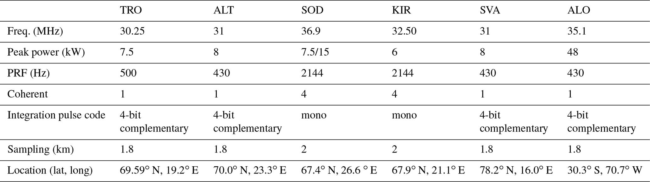
The second meteor radar network is called Chilean Observation Network De Meteor Radars (CONDOR) and employs a monostatic radar at the Andes Lidar Observatory (ALO), a passive receiver at the Southern Cross Observatory (SCO) and another passive receiver at Las Campanas Observatory (LCO). Based on these data sets, we demonstrate the utility of the technique with a series of case studies of body forces, vortices and other spatial features that are not observable by other techniques so far. Furthermore, we show a keogram analysis of a minor sudden stratospheric warming (SSW) in December 2019 and the latitudinal resolved tidal response. Finally, we demonstrate the possibility to obtain horizontal wavelength spectra as already outlined in Stober et al. (2018a).
The paper is structured as follows. The Nordic Meteor Radar Cluster and CONDOR are described in Sect. 2. Section 3 provides a detailed presentation of the wind retrievals, the World Geodetic System 84 (WGS84) geometry, forward scatter solvers and the optimal estimation technique, which includes the concept of measurement response, variable geographic and Cartesian grids. The performance of the algorithm is demonstrated in Sect. 4, showing examples of body forces, horizontal wavelength spectra and keogram analysis. The results of the retrieval are discussed in Sect. 5, and conclusions are drawn in Sect. 6.
Meteor radar (MR) observations have become a standard tool to investigate MLT dynamics such as winds, tides, GWs and GW momentum fluxes (e.g., Hocking et al., 2001; Holdsworth et al., 2004; Fritts et al., 2010; Pancheva et al., 2020; Spargo et al., 2019; Stober et al., 2021; Dempsey et al., 2021). These radars are designed for continuous and unattended operation under various climate conditions, making them ideal for remote deployments. However, MRs require a rather large field of view of up to 400 km in diameter to detect a sufficient number of meteors, which occur randomly in space and time, to estimate the instantaneous 3-D winds.
All MRs used in this study have very similar designs and operation principles, although they are manufactured by two different companies: ATRAD Ltd. (Holdsworth et al., 2004) and Genesis Ltd. (Hocking et al., 2001). The systems utilize a single Yagi antenna for transmission and on reception an asymmetric cross, a so-called Jones array (Jacobs and Ralston, 1981; Jones et al., 1998), with an antenna spacing of 1 and 1.5 λ and 2 and 2.5 λ. Only the MR at ALT in northern Norway employs a receiver array with 1 and 1.5 λ antenna spacing. Further details about the transmitter power, frequency and experiment settings are summarized in Table 1. The passive receiver stations in Chile are also in a Jones array with the standard spacing of 2 and 2.5 λ. Besides, all CONDOR stations are further equipped with rubidium-disciplined GPS to ensure a high frequency and time coherence between the transmitter and the remote receivers.
Figure 1 shows two map projections of the Nordic Meteor Radar Cluster and CONDOR with color-coded elevation. CONDOR stations are located at the windward side of the Andes; the Nordic Meteor Radar Cluster stations are distributed across northern Scandinavia. Eastward winds in both regions favor the excitation of mountain waves that propagate deeply into the thermosphere. Due to local instabilities and momentum deposition, secondary waves are excited.
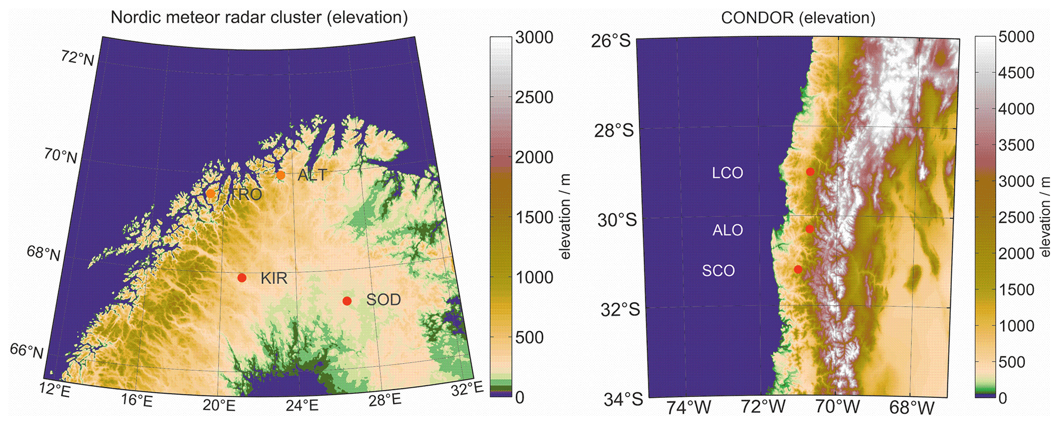
Figure 1Nordic Meteor Radar Cluster and CONDOR locations visualized with color-coded mean elevation. The maps were generated from etopo1 using the m_map package (Amante and Eakins, 2009).
Meteoroids entering the Earth's atmosphere are decelerated and heated by collisions with the ambient atmospheric molecules. Some of them, which have sufficient kinetic energy, are vaporized forming an ambipolar diffusing plasma column, which is called a meteor. MRs measure the line of sight or radial velocity of specular meteor trails that drift with the wind. The position of the meteor in the sky relative to the radar is determined by interferometry and typically given as azimuth and off-zenith angles. MRs have wide fields of view and thus large observation volumes, making them ideal scientific instruments to infer the spatial characteristics of atmospheric parameters.
3.1 Meteor radar winds
Instantaneous winds are often derived by applying so-called all-sky fits (Hocking et al., 2001; Holdsworth et al., 2004) for pre-defined time and altitude intervals. Therefore, the data are sorted into altitude–time bins, and a zonal and a meridional wind value is fitted using least squares by minimizing a function of merit, or cost function, which is given by the radial wind equation:
Here, vr denotes the observed radial velocity, u, v and w are the zonal, meridional and vertical wind components, and ϕ and θ denote the azimuth and off-zenith angle at the geodetic coordinates of the meteor (Stober et al., 2018a). An alternative expression is obtained from the angular Doppler frequency wd (rad s−1), the Bragg vector k and the wind vector u;
Doppler frequency fd (Hz) and the angular Doppler frequency are related by wd=2πfd. The Bragg vector is given by with , where λ is the radar wavelength and λB describes the Bragg wavelength. We will get back to the Bragg notation when discussing the forward scatter geometry for CONDOR. However, the tomographic wind retrieval is making use of the notation of the radial wind equation only, as it depends on physical and geometric parameters and not on the observational technique or radar-specific quantities such as the wavelength or Bragg vector.
Very often MR horizontal winds are obtained under the assumption of w=0 m s−1, which is reasonable considering the large observation volume at the MLT of about 400 km in diameter (Hocking et al., 2001; Holdsworth et al., 2004). However, in this study, we explicitly consider/solve for the vertical wind and actually estimate the residual bias to assess whether the assumption of a negligible vertical wind holds. We apply the retrievals as presented in Stober et al. (2018a), which includes a full non-linear error propagation (Gudadze et al., 2019), a spatiotemporal Laplace filter and a WGS84 reference ellipsoid Earth geometry. The spatiotemporal Laplace filter is beneficial to reduce a potential ill conditioning of the wind fit due to the random occurrence of meteors inside the observation volume. Only a few meteors enter the analysis at the upper and lower altitudes of the meteor layer. The spatial distributions there might not allow to derive all wind components with a good measurement response, resulting in large errors and systematic biases. The spatiotemporal Laplace filter uses a derivative in time and altitude to ensure mathematical smoothness and thus reduces the ill conditioning and potential biases. The WGS84 geometry further minimizes altitude and projection errors on the wind components.
The residual bias for both networks is shown in Fig. 2.
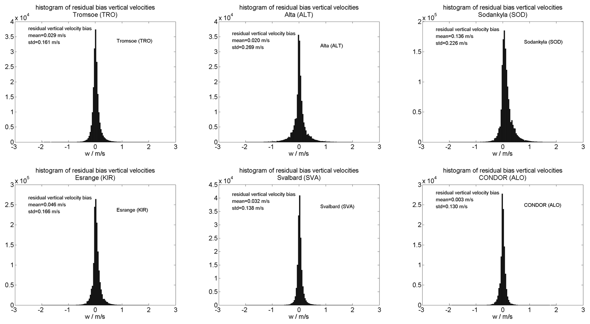
Figure 2Histograms of the residual vertical wind bias for TRO, ALT, SOD, KIR, SVA and ALO MR.
The histograms are estimated from hourly winds and interpreted as mean residual bias due to the lack of a reliable validation possibility. We observed typical biases of a few cm s−1 and a standard deviation of about 15–25 cm s−1. This quality control helps to remove systematic issues in the interferometric solutions caused by mutual antenna coupling by the surrounding radar hardware. Based on these histograms, we accepted only meteor detections within an off-zenith angle of 65∘ for TRO, SVA, SOD and KIR as well as CONDOR. For the ALT site, we used a more strict criterion of a 55∘ off-zenith angle, as we found systematic deviations for meteors at lower elevation. The inclusion of these meteors was leading to a substantial skewness of the vertical velocity histogram towards positive values, which almost disappeared when using the more limited off-zenith angle range.
3.2 Implementing the WGS84 reference ellipsoid
Due to the large observational volume covered by the multistatic MR networks of the Nordic Meteor Radar Cluster and CONDOR, a realistic representation of the Earth's shape is required. Otherwise, large projection errors could result in significant biases. A good approximation of the Earth's shape is given by the WGS84 reference ellipsoid (National Imagery and Mapping Agency, 2000). A detailed description of how to implement the WGS84 into the MR wind analysis was outlined in Stober et al. (2018a). The all-sky fits described by Hocking et al. (2001) included a correction for the Earth's curvature of the computed meteor altitudes and wind estimates by using a mean Earth radius and spherical geometry.
Here, we briefly summarize how the WGS84 geometry is considered in the wind retrieval. All involved coordinate transformations are given in Appendix A (Zhu, 1993; Heikkinnen, 1982). MRs determine the angle of arrival relative to their geodetic geographic position in the east–north–up (ENU) coordinate frame. Meteors are typically observed at distances between 80 and 220 km for off-zenith angles up to 65∘. The Earth's curvature has to be taken into account when estimating the altitude above the Earth's surface (Hocking et al., 2001; Stober et al., 2018a). However, there is also a non-negligible difference between the ENU coordinates at the radar location and the ENU coordinates at the geodetic position of the meteor itself, which has to be considered in the radial wind equation. Therefore, we have performed a coordinate transformation of all line-of-sight velocities from the ENU coordinate frame of the radar to the ENU coordinate frame of the meteor according to the following steps:
-
transform geodetic radar coordinates into Earth-centered–Earth-fixed (ECEF) coordinates using transformation geodetic to ECEF (A1);
-
determine ECEF coordinates of meteor position using transformation ENU to ECEF (A3);
-
transform ECEF meteor position coordinates into the geodetic location of the meteor using transformation ECEF to geodetic (A2); and
-
transform observed line-of-sight velocity into the ENU coordinate frame at the meteor location using transformation ECEF to ENU (A4).
The implementation of the WGS84 Earth geometry turned out to be important for all meteor wind analyses, and it essentially reduces the projection and altitude biases of the observed meteors. In particular, at midlatitudes and high latitudes, these corrections are rather significant and lead to substantial improvements of the wind as well as the vertical profile of ambipolar diffusion and thus has an impact on the temperature estimates (Hocking, 1999; Hocking et al., 2001). Furthermore, the vertical wind mean bias and variances are significantly reduced compared to other studies (Egito et al., 2016; Chau et al., 2021; Conte et al., 2021) without including additional damping terms or regularization constraints to the fitted vertical wind as was the case in previous studies (Stober et al., 2017; Wilhelm et al., 2017). However, our solver prefers a smaller norm, which apparently is associated with small vertical winds. The algorithm was validated against ECMWF-forecast data using the Middle Atmosphere Alomar Radar System (Latteck et al., 2012) and reached a correlation coefficient of 0.984–0.994 and a slope of 0.987–0.998 (Stober, 2020).
3.3 CONDOR forward scatter geometry
Here, we briefly review the forward scatter position determination for multistatic meteor radar observations such as CONDOR. In ASGARD, we updated the algorithm to be more general and applicable to arbitrary meteor radar networks. In Fig. 3, we show a schematic representation of the multistatic geometry and a map of CONDOR presenting the locations of the three stations (ALO, SCO and LCO; red dots in the right panel) and intersection points of the observed Bragg vectors with the distance vector (small blue dots in the right panel).
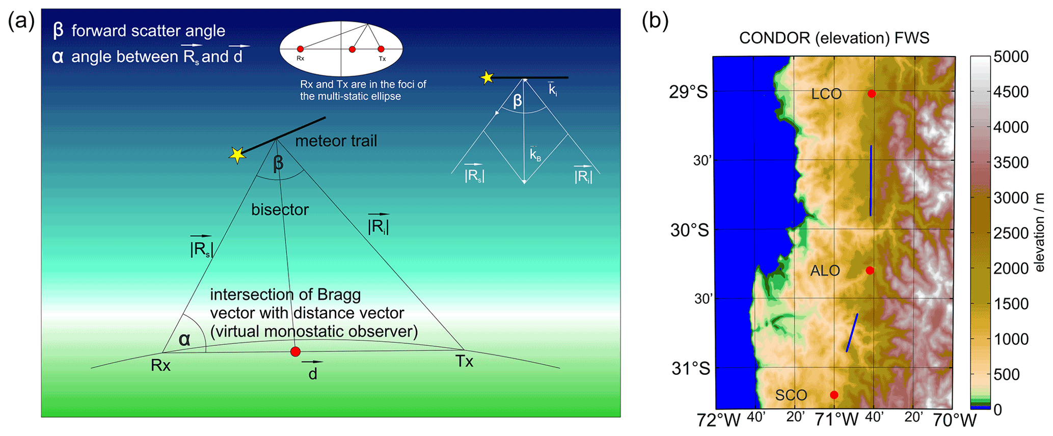
Figure 3(a) Schematic representation of the forward scatter geometry and Bragg vector for CONDOR. (b) Geographic map of CONDOR with the active and passive radar locations at ALO, SCO and LCO (red dots). The two sets of intersection points of the Bragg vectors with the distance vector between Rx and Tx are shown as blue dots, which are only visible as two blue streaks due to the close proximity of the intersection points.
CONDOR is located at the Andes and some stations are installed at considerable high altitude. The geodetic positions of the transmitter (Tx) at ALO (30.251944∘ S, 70.737778∘ W; mean sea level (m.s.l.) altitude 2520.0 m) and the passive receivers (Rx) at SCO (31.200834∘ S, 71.000000∘ W; m.s.l. altitude 1140.0 m) and LCO (29.021666∘ S, 70.689720∘ W; m.s.l. altitude 2339.0 m) are known. At each station, the meteor position is determined as the angle of arrival in the ENU frame of reference at the geodetic location of the Rx. The distance vectors d are computed in ECEF coordinates and then transformed into the ENU frame of reference at the Rx sites. The SCO station is about 108.2 km south of ALO and the azimuth (ϕ) and off-zenith (θ) angles are ϕ=76.51∘ and θ=89.76∘. The northern CONDOR site at LCO is 136.5 km away from the Tx and the local ENU azimuth and off-zenith angle are ϕ=268.05∘ and θ=90.54∘. The off-zenith angles are almost, but not exactly, 90∘. The deviations are mostly due to the altitude difference of the Tx compared to the Rx locations and reflect the unique environment for such an installation compared to the multistatic network in Germany (Stober and Chau, 2015; Stober et al., 2018a).
In the next step, we solve the multistatic geometry and determine the Bragg vector, which lies within the plane spanned by the meteor, Rx and Tx locations. The angle α shown in Fig. 3 denotes the angle between the unit vector from the Rx site to the meteor position in the sky in the ENU frame of reference (Rs) and the distance vector to the Tx:
Furthermore, we measure the total range at the receiver station, which for a monostatic system is 2 times the monostatic range commonly stored in the data stream. However, multistatic links are often further away and thus the signal may travel for a time longer than an interpulse period before reaching the receiver. Therefore, we compute solutions considering a potential range aliasing due to the employed pulse repetition frequency (PRF) of the experiment and convert these into a range R0. The total range then becomes a function of an integer number of the measured range (Rge) and the R0 range:
We now solve n times the arbitrary triangle equation for Rs
The result is an ensemble solution for Rs(n), which can be easily converted to potential meteor altitudes by analogy with the algorithm presented above for monostatic cases. However, only one solution is correct and physically meaningful and kept for all further analysis. That is, we only consider solutions in the altitude range between 70 to 120 km and pick the one with the smallest absolute altitude difference to 91 km.
The Bragg vector is derived by transforming the Tx, Rx and meteor positions in ECEF coordinates and by computing the forward scatter angle β, which is defined as the angle between the vectors Rs and Ri. The bisector is given by and lies in the same plane spanned by the points Tx, Rx and the meteor and defines the direction of the Bragg vector. The magnitude corresponds to the radial velocity along the Bragg vector. Similar to the range, the standard radar software often provides a monostatic radial velocity measurement , which has to be corrected for the forward scatter geometry by
Here, λ is the radar wavelength, vr is the monostatic radial measurement obtained from the Doppler frequency fd (Hz), and vrad describes the radial velocity along the Bragg vector. By analogy, we correct the radial velocity error to account for the forward scatter geometry as well.
Finally, we compute the intersection point between the Bragg vector and the distance vector to perform a sanity check. In Fig. 3b, we show these positions as blue points for 3 d. All points are found between the Tx and Rx sites and form streaks around the midpoints between the Tx and Rx locations. The longer the distance vector becomes, the longer the streak.
3.4 Optimal estimation 2D-Var/3D-Var wind retrieval
Atmospheric tomography from multistatic meteor radar networks demands sophisticated mathematical approaches because the number of unknowns exceeds the number of observations. There are several strategies to solve such ill-posed and often ill-conditioned problems by assuming a certain smoothness of the solution or other constraints to cure the mathematical rank deficiency of the problem. Optimal estimation is a technique often applied for atmospheric remote sounding and is described in detail in Rodgers (2000). The optimal estimation technique has become a standard tool in radiometry to retrieve atmospheric quantities such as wind, temperature or trace gas concentration (Livesey et al., 2006; Schwartz et al., 2008; Stähli et al., 2013; Hagen et al., 2018; Schranz et al., 2020; Navas-Guzmán et al., 2016)
The optimal estimation technique makes use of Bayes' theorem and presents a general view to all solutions of an inverse problem (Rodgers, 2000). The Bayesian approach relates the posteriori probability density function (PDF) for a given measurement using prior knowledge of the PDF of the state x and observations y before a measurement is made. The forward model maps the state space onto the measurements. These PDFs are often approximated using Gaussian statistics for the measurement error, which appears to be appropriate for many inverse problems.
The 2D-Var/3D-Var wind retrievals are implemented using a posteriori PDF covariance Sx given by
Here, is the a priori covariance matrix, which also includes the correlation lengths ( norm) and has full rank, Sy denotes the measurement covariances, and A is the Jacobian of our forward model and is often rank deficient (there are fewer observations than unknowns). Furthermore, we know an a priori state xa of our forward model, which is updated using the posteriori and measurement covariances, the forward model at the a priori state xa, and the observations y is expressed as
Considering a typical tomographic domain area with 20 by 20 pixels/grid cells in longitude and latitude, and 20 vertical layers between 70–110 km, results in a large and highly sparse matrix of , which has a block diagonal shape. Instead of solving such a large matrix by brute force, as a first step, we divide the problem into several smaller blocks. Each block corresponds to a horizontal layer (2D-Var). In a second iteration, we add the vertical coupling for all grid points with observations by adding an additional cost to the inverse problem (3D-Var). This cost is estimated by computing the vertical derivative between the layer above and below or, at the domain boundaries, between the layer itself and the one above or below. Vertical layers without any meteor observations are omitted. We implemented a user defined threshold for the minimum number of meteors in one layer to still be retrieved. This was tested with as low as six meteors, but it turned out to be more beneficial to use at least 10 to 15 meteors. In total, we perform eight iterations mainly to include a non-linear error propagation similar to Gudadze et al. (2019) and to update the 3D-Var vertical cost function. However, the a priori data and a priori covariances are not updated between the iterations.
The forward model in the retrieval is given by the radial wind Eq. (1) in ENU coordinates at the geodetic position of each meteor. The standard error is assumed to be 20 m s−1 for the horizontal wind components and about 5 m s−1 for the vertical wind. However, as the choice of the standard error also depends on the measurement statistics and thus is a function of the temporal and spatial resolution of the retrievals, we introduced a Lagrange multiplier to control the smoothness constraint α2. By default the vertical smoothness is one-fourth of the horizontal coupling strength to avoid a too-strong instability growth at the upper and lower edges of the meteor layer, when only a few meteors enter the retrieval, and to account for the possibility to use different smoothness constraints and to scale the a priori covariances. Typical values are in the range of α2=0.02 to 1.
We also implemented an option to include longer correlations or polynomial structure functions, which satisfy L2 norms. The software offers to use correlations of , , , but the default is always an matrix as shown in Stober et al. (2018a). The subscript stands for the norm and the superscript for the correlation length. However, these higher-order correlation functions, which are basically spatial derivatives, tend to show an exponential growth at the domain boundaries, which appears to be unrealistic. These functions may be more important when larger domain areas are combined and there is no longer a direct overlap between the observation volumes. Furthermore, the increased spatial correlation is only available in the horizontal domain. The vertical coupling is fixed to the next upper or lower layer, which appears to be most realistic considering the vertical shears induced by atmospheric waves, e.g., tidal waves and GWs.
3.5 Cartesian and geographic grids
The tomographic retrieval domains can be user defined. Therefore, we implemented two geographic coordinate systems based on a Cartesian and a geographic grid. The Cartesian grid is represented by a geographic longitude and latitude, which defines a xy coordinate (0,0). All other grid points are measured from this reference in the north–south or east–west direction defining a rectangular grid (Stober et al., 2018a). The geographic grid is given by defining longitude and latitude boundaries and a latitudinal and longitudinal increment. Both grids use as a vertical coordinate the height above the WGS84 reference ellipsoid.
Furthermore, we have to define voxels for each grid point. The default voxel is a cylinder with radius and height h. The variable d denotes the grid resolution for the Cartesian grid. The same voxel shape is applied to the geographic grid, but the radius is configured to a specific value, which is typically estimated for a certain latitude in the domain to ensure a proper coverage and overlap. Due to the Earth's shape, the effective voxel volume increases with increasing altitude, and we keep for each grid cell a fixed longitude and latitude independent of the coordinate grid. The cylindrical shape of the voxel also results in overlapping regions between adjacent grid cells, in particular for the Cartesian grid. However, meteors falling within these overlapping regions are basically detected between two grid cells and hence are included in both with the same weight.
In Fig. 4, we show two retrieval results using the Cartesian and geographic grid for the same time and altitude and a difference plot after remapping the geographic wind field to the Cartesian grid. The horizontal wind strength is color coded and the orange arrows label the prevailing wind direction for all grid cells, where a meteor was observed. Please note that the wind arrows are always plotted at the grid cell center, which could lead to some shifts of half a grid cell diameter between the two projections. Grid cells that are not driven by observations are just showing the color-coded wind strength, and these retrieval solutions are mostly driven by longer correlation lengths and are the result of extrapolations or interpolations. Both retrievals show that the mean wind field is well reproduced and many features are recovered in both grids. Larger dissimilarities occur towards the domain boundaries, where no observations are available. In particular, the body forcing event around the geographic coordinates (69.5∘ N, 20∘ E) is found in both images showing an acceleration of the mean flow towards southeast and two counter-rotating vortices indicated by a weakening of the wind strength north and south of the forcing region. Body forces are discussed in more detail in Sect. 4.1.
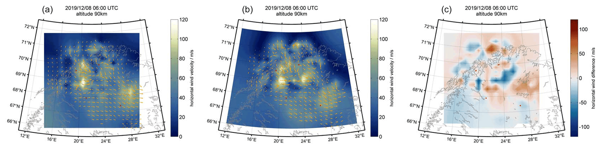
Figure 4Image of 3D-Var retrieved wind fields obtained above the Nordic Meteor Radar Cluster using a Cartesian grid (a) and a longitude–latitude geographic grid (b). The gray line represents the Nordic coast. The orange arrows denote wind direction and the color bar represents the wind magnitude. Panel (c) shows a difference plot between both retrievals after remapping the geographic to the Cartesian grid using cubic interpolation.
The difference plot shows the variability between both retrievals and provide an estimate on the spatial variance due to the different grids. We obtained a variance of about 20 m s−1 that is on the order of a typical horizontal wind shear between neighbor grid cells and a median offset of 0.3 m s−1 between both retrievals considering the whole domain. However, we note that the cubic interpolation between the grids added an additional variability and caused an inflation of the variance that is difficult to assess. Furthermore, we point out that we always plot the wind arrows at the center of a grid cell, which might be not the statistical median position in some part of the domain area due to the sparsity of the observations.
3.6 Shannon measurement response
Shannon and Weaver (1949) provide the mathematical entropy definition for the information content, which is basically the same as the Gibbs definition of the thermodynamic entropy besides a constant factor k:
Here, S is the entropy and pi describes the probability of being in state i. In thermodynamics, k is the Boltzmann constant and in information theory k=1. Considering that we have one state before a measurement and one after, the change in entropy is given by
The information gain during the retrieval is an important measure and has direct practical implications. We basically want to know how the a priori knowledge is improved by the observations. The averaging kernel R is another important quantity as it contains information about the information correlation and measurement response for each grid cell and retrieved parameter:
For linear Gaussian PDFs, the information entropy change is linked to the averaging kernel by
The measurement response is obtained by integrating all non-negligible contributions from the averaging kernel for a retrieved quantity at a certain altitude and time bin. Examples of such averaging kernels and the corresponding measurement responses have been presented for ground-based radiometer observations (Hagen et al., 2018) and for satellites, e.g., the Microwave Limb Sounder (MLS) (Livesey et al., 2006; Schwartz et al., 2008). Although it is desirable to keep the averaging kernels for the 3D-Var wind retrievals, storing a full rank matrix for each retrieved quantity and time–altitude bin is not very practical. Due to the random occurrence of meteors, the measurement response and the corresponding width of the averaging kernel changes for each grid cell and retrieved quantity for a given time–altitude bin.
Furthermore, there is a major dissimilarity between the integral (line-of-sight) irradiance observations from satellites or ground-based radiometers and the differential meteor observations, which have a well-defined location. This has an important implication for the interpretation of the width of the averaging kernel for a given grid cell and retrieved quantity in the 3D-Var retrieval. An increased width of the averaging kernel reflects an interpolation/extrapolation of information from more remote grid cells. From Fig. 4, it is obvious that also grid cells at the domain boundary, where no meteors are detected even in the surrounding grid cells, are driven by the observations from grid cells that are further away, implying long correlations and thus a still-high measurement response when integrating over the width of the averaging kernel. However, we defined an a priori correlation length, and thus we compute the measurement response only for short correlations. This results in low measurement responses for grid cells with an increased width of the averaging kernel and a high measurement response for grid cells with narrow averaging kernels.
In Fig. 5, we show an example of 3D-Var retrieved wind fields and the corresponding measurement response for an observation in March 2020 from CONDOR. The zonal and meridional wind magnitudes are typical for the time of the day and the season. The wind structures are dominated by the diurnal tide. The zonal and meridional winds are presented as color-coded strength. Reddish colors indicate eastward and northward winds while bluish colors show westward and southward winds, respectively. The measurement response is provided as color-coded intensity. A measurement response close to 1 represents an entirely data-driven solution. There may even be measurement responses much larger than 1, which point towards even narrower averaging kernels than assumed in the a priori covariance. The orange and yellow lines correspond to measurement responses of 0.7 and 0.4. The whitish colors reflect a high measurement response, whereas bluish colors point towards increased averaging kernels corresponding to a decreased measurement response. However, these points are still driven by the observations rather than the a priori covariance. The measurement response for CONDOR clearly reflects the layout of the meteor radar network with a preference towards north–south. This setup results in a high measurement response for the meridional component above the sites in the north–south direction but a decreased capability to retrieve zonal winds. However, the zonal component clearly shows two regions towards the east and west of the radar sites, which indicate a very high measurement response. The measurement response clearly reflects the radial nature of the forward model for the retrieval and the meteor radar network setup. Furthermore, the maps of measurement response indicate the differences between the typical response of monostatic systems compared to passive multistatic receivers. Passive radar links have very distinct sampling responses that are not equivalent to monostatic radars and much less isotropic.
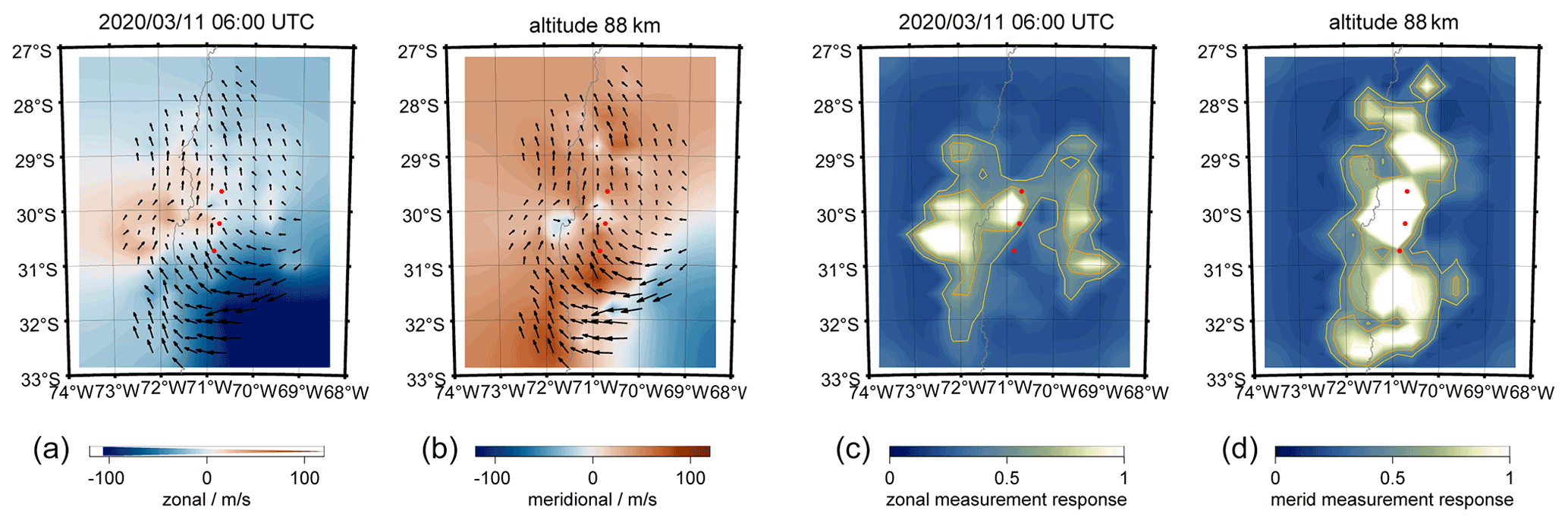
Figure 5Panels (a) and (b) show the color-coded zonal and meridional wind strength. Bluish colors indicate southward and westward motions; reddish colors highlight northward or eastward winds. Black arrows show the wind direction centered at each grid cell. Panels (c) and (d) show the color-coded measurement response for the zonal and meridional wind components.
For the Nordic Meteor Radar Cluster, an example of the observed 3D-Var wind field and the corresponding measurement response is shown in Fig. 6. The map of the zonal and meridional measurement responses reflects again the radial nature of the forward model for the wind retrieval. Meridional winds have high measurement responses north and south of the radar locations and the zonal wind is most reliably retrieved in the east–west direction, respectively. Furthermore, the measurement response maps indicate how the different systems complement each other. In particular, TRO, ALT and KIR have a sufficient volume overlap and angular diversity to generate a larger patch with a high measurement response for both wind components (geographic overlap of whitish areas). SOD is located a bit more to the south and east of the cluster, and thus the typical measurement response is only high for a certain wind component and geographic area.
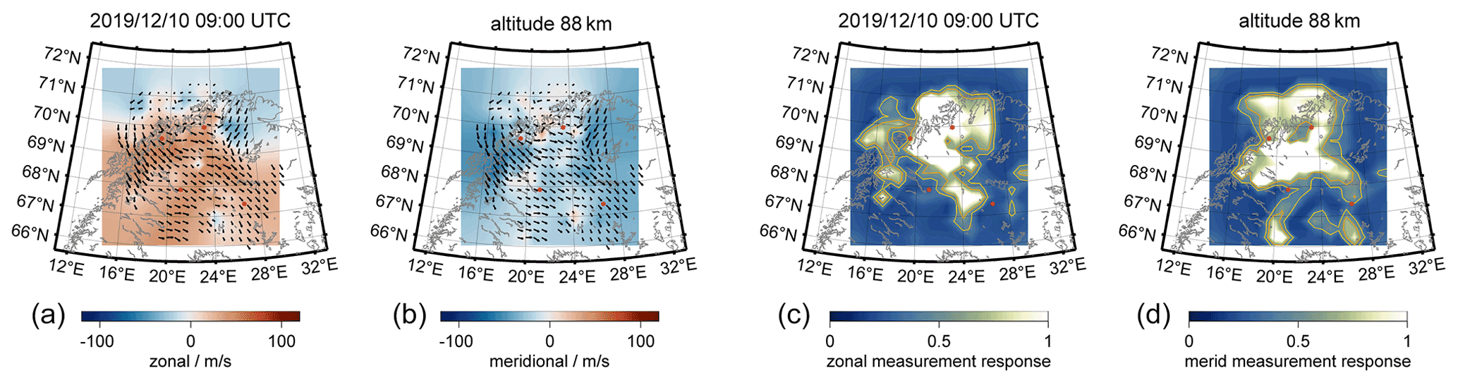
Figure 6The same as Fig. 5 but for the Nordic Meteor Radar Cluster.
3.7 Data assimilation and a priori state vector
ASGARD offers several possibilities for the a priori state vector. However, considering the optimal estimation technique and the properties of the forward model, which is linear in all coefficients, the final impact of the retrieved parameters appears to be almost independent of the choice of the a priori state vector for all grid cells. This is a major benefit compared to previous retrievals presented in Stober et al. (2018a), where the a priori choice of the state vector did impact parameters with a low measurement response in certain areas of the domain.
There are three options available. The first option is a zero-wind state vector for all wind components. The second option is a mean wind vector for the horizontal wind and w=0 m s−1. Finally, the third option is a data assimilation wind field, which is estimated from a distance-weighted single station wind retrieval or using satellite data, e.g., TIDI (Wu et al., 2006) assuming again w=0 m s−1. A potential satellite data assimilation appeared to have little impact considering the uncertainty in the geographic location of the observations and the recommended temporal averaging and thus was omitted in the current retrievals. However, it is likely worth including over larger or global retrieval domains. All wind fields presented in this paper used the data assimilation approach.
4.1 Body forces and vortices
Gravity wave dynamics is a vital topic of research. The 3D-Var wind retrievals allow us to study new aspects of spatially and temporally resolved GWs and their interaction with the mean flow. Vadas and Fritts (2001) investigated body forces of breaking GWs and the resulting flow responses with a model. The resulting body forces were characterized by two counter-rotating vortices and a strong acceleration region between them assuming a zero mean background flow.
Recently, there have been several studies on secondary GW generation due to such body forces using a mechanistic model above the Andes and Antarctic Peninsula (Becker and Vadas, 2018; Vadas and Becker, 2018). These secondary-generated GWs resulted in significant changes to the momentum fluxes at the MLT above these regions, which was confirmed by meteor radar observations of the momentum fluxes and wind variances (Dempsey et al., 2021; Stober et al., 2021).
Figure 7 shows a body forcing example of a breaking GW at the MLT above the Andes. Our searching strategy for such events is based on two data products. First, we screen the zonal and meridional winds for enhancements or decreases in the mean flow. In a second step, we investigate the wind residuum to identify two counter-rotating vortices. The wind residuum is estimated by subtracting the mean flow from the images, which is estimated as the median zonal and meridional wind considering the whole domain area. The event in Fig. 7 is visible at two altitudes, occurred at approximately 89 km and had a vertical depth of approximately 3–4 km. The forcing region is indicated by a red circle in panel (a) and the yellow arrow points towards the main forcing direction. The body force is deposited in an area of approximately 90–120 km in diameter (three to four grid cells) and shows a westward acceleration, which leads to a weakening of the strong eastward winds in the forcing region. Panel (b) reflects two counter-rotating vortices north and south of the forcing region. The circular white arrows visualize the rotation direction. Panels (c) and (d) present the same event but at an altitude of 90 km.
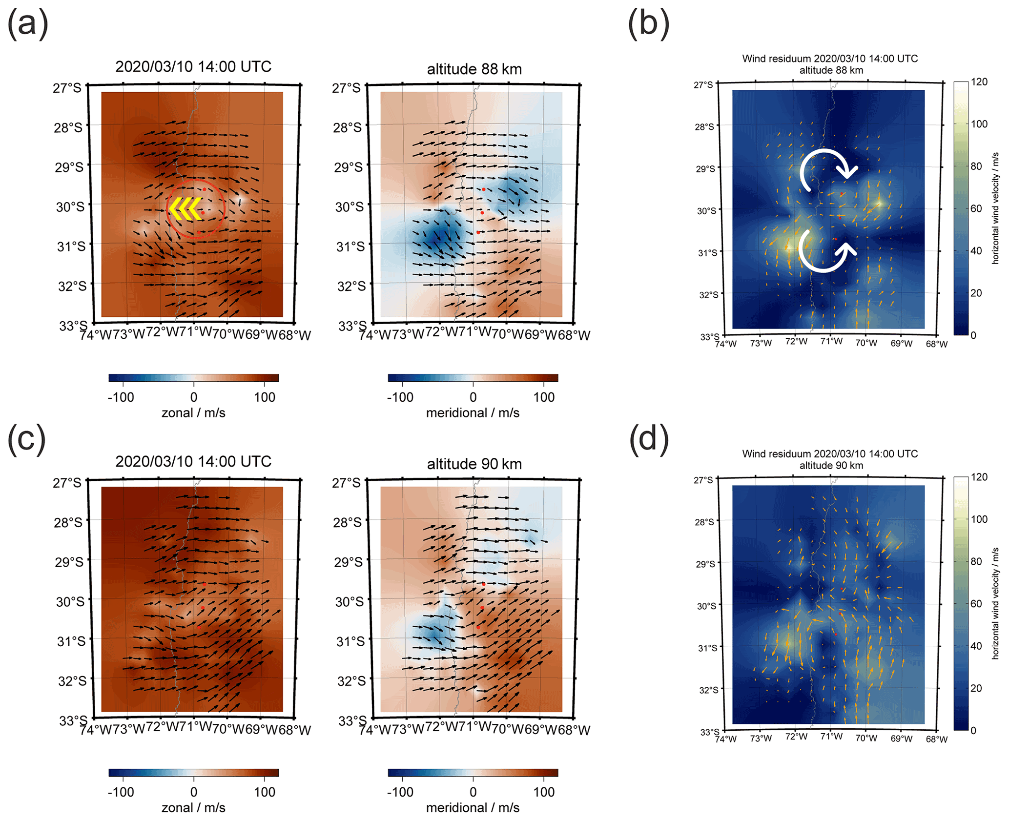
Figure 7Body force of a breaking gravity wave above CONDOR. Panels (a) and (c) show the zonal and meridional components at 88 and 90 km. Panels (b) and (d) visualize the two counter-rotating vortices after subtraction of the domain mean zonal and meridional wind. The body forcing event is indicated by a red circle, the forcing direction is given by a yellow arrow (a), and the two vortices and their rotation direction are presented by white arrows (b).
The spatial and vertical dimensions of the vortices and the forcing region are in good agreement with the theoretical work of Vadas and Fritts (2001) and provide confidence in the retrieval results. The vortical structures and forcing region are in areas with a measurement response greater than 0.7 (see Fig. 8). We find similar body forcing events for the Nordic Meteor Radar Cluster (see Fig. 4).

Figure 8The four panels show the measurement response for the zonal and meridional wind components and both altitudes of the body force event above CONDOR.
A major benefit of multistatic observations is the imaging capabilities of large-scale features such as vortices, which remain hidden in monostatic measurements. CONDOR is located at a scientifically interesting region between the low latitudes and midlatitudes. We very often observe strong regional-scale shears in the zonal and meridional wind components associated with vortices. Figure 9 shows a vortex embedded in a large-scale shear flow of a type that is occasionally found above CONDOR. This vortex exhibits a diameter of approximately 300 km. Due to the limited domain size, we are not able to distinguish whether the vortex was the result of a large-scale body force or of a large-scale shear in the zonal component between the equatorial latitudes and midlatitudes.
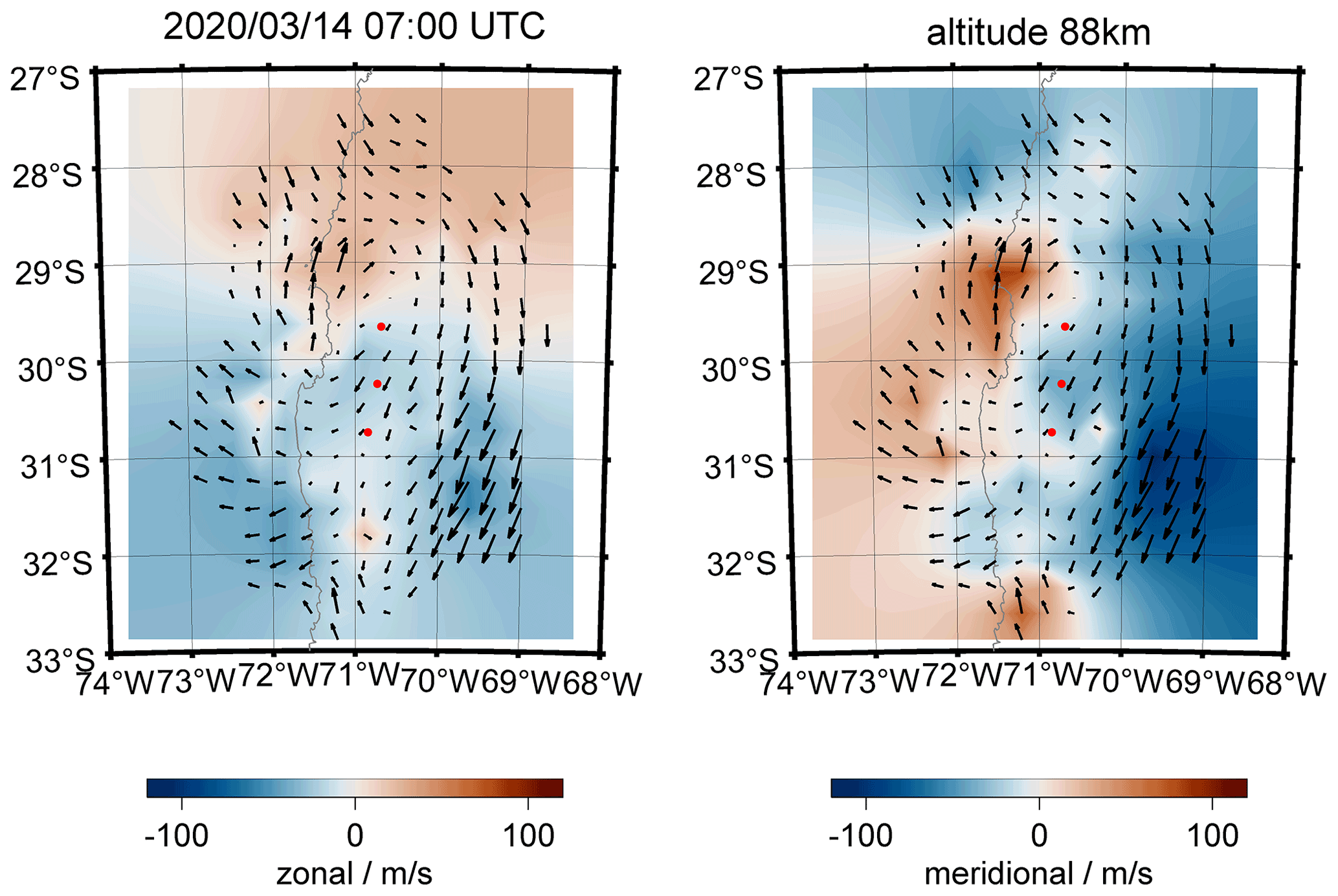
Figure 9The two panels present color-coded 3D-Var retrievals of zonal and meridional winds. The black arrows highlight a large vortex above the Andes observed on 14 March 2020.
4.2 Large-scale regional dynamics and keogram analysis
Besides the GW dynamics, the 3D-Var retrieval also captures spatial information of the regional effects of larger-scale dynamics such as sudden stratospheric warmings or atmospheric tides and planetary waves. The 3D-Var retrieval results in a significant increase of the available information within the domain area. For a temporal resolution of 1 h and a vertical resolution of about 2 km between 70–110 km altitude, we obtain about 480 images per day. If we analyze the wind fields at 10 min resolution, which was occasionally achievable, we generate 2880 images per day. However, for atmospheric tides and planetary waves, it is sufficient to look at certain cross sections of the domain area. This can be achieved by keogram analysis, which provides information about the wind dynamics at the temporal evolution for a given longitude and altitude. Here, we present altitude–time–wind (ATW) plots, which either show the mean winds over the domain area or at a specific longitude and latitude.
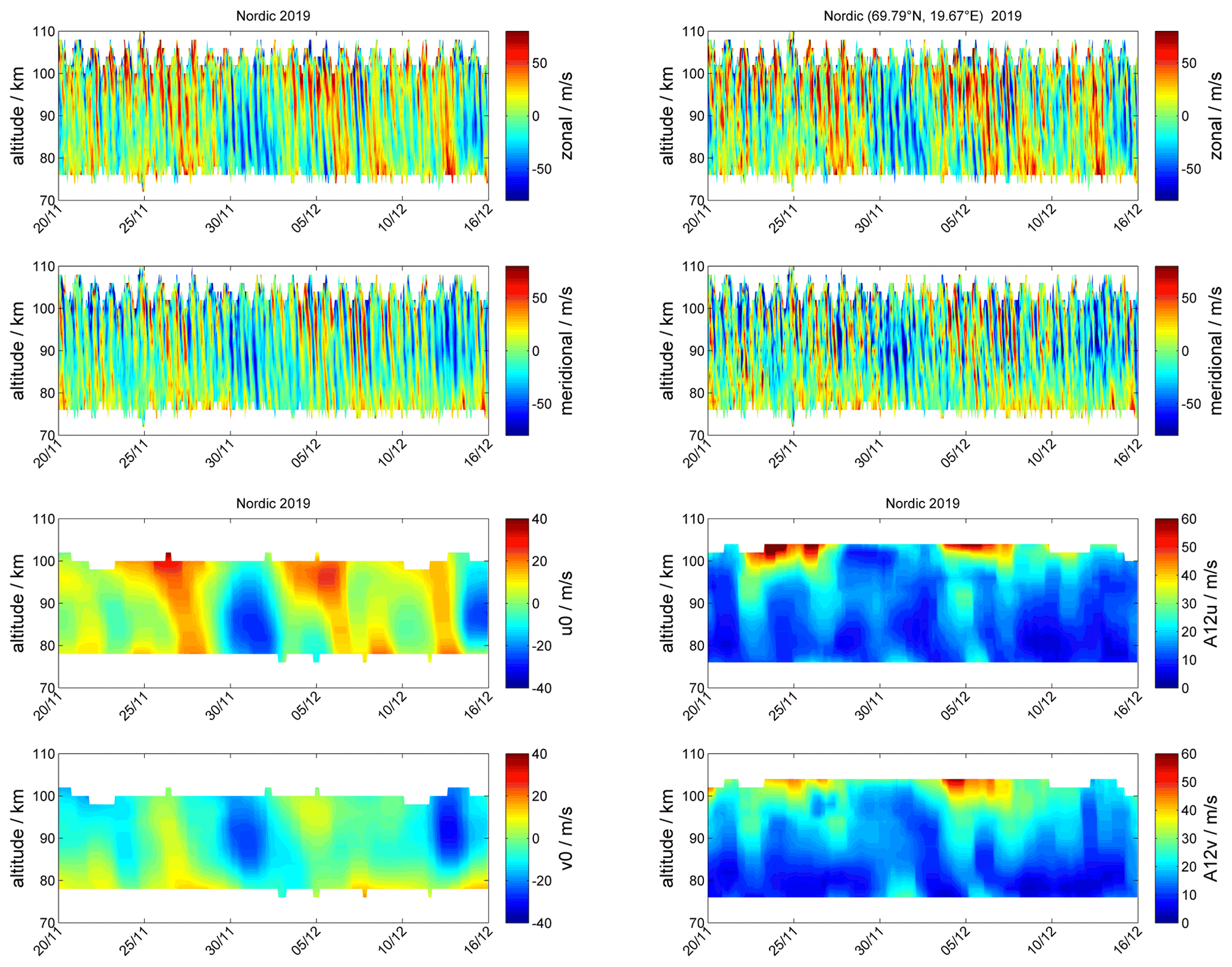
Figure 10The two left panels show altitude–time–wind (ATW) plots for the zonal and meridional color-coded wind strength integrated over the Nordic domain from 20 November to 15 December 2019. The two right panels highlight the zonal and meridional wind strength for the grid cell located around geographic latitude (69.79∘ N, 19.67∘ E) for the same period. The two lower rows show the daily mean zonal and meridional wind (left) and the daily semidiurnal tide amplitude for both wind components (right).
In Fig. 10, we show ATWs for the Nordic Meteor Radar Cluster from 20 November to 15 December 2019, daily mean winds and semidiurnal tidal amplitudes, and in Fig. 12 the corresponding keograms for the same period at an altitude of 90 km and longitude of 22∘ E. During this period, we observe an early minor stratospheric warming around the beginning of December (bluish colors). Furthermore, there is a strong semidiurnal tidal activity, which enhances after the minor warming that occurred at the beginning of December and exhibits an obvious day-to-day variability indicating increased amplitudes during mean eastward winds and inhibited amplitudes for times with more intense westward winds. The left ATW in Fig. 10 shows median zonal and meridional winds over the entire domain area, whereas the right panel presents the winds in the column above the grid cell at the geographic location (69.79∘ N, 19.67∘ E). Both ATWs reflect the same large-scale dynamical situation with a dominating semidiurnal tide, but the ATW above a single grid cell also highlights the presence of enhanced GW activity, which is removed by averaging the winds over the domain area. Furthermore, Fig. 11 presents GW residuals after removing daily mean winds as well as diurnal and semidiurnal tides, which highlights the increased GW activity in the grid cell data compared to the domain average for all waves with periods between 1–11 h. The filtering was done using the adaptive spectral filter (ASF) approach presented in Baumgarten and Stober (2019), Stober et al. (2020).

Figure 11Panels (a) and (c) show the zonal and meridional gravity wave residuum for all waves in the period range between 1 and 11 h with color-coded amplitude integrated over the Nordic domain from 20 November to 15 December 2019. Panels (b) and (d) highlight the same but for the grid cell located around geographic latitude (69.79∘ N, 19.67∘ E) down to horizontal scales of 60 km.
The keograms in Fig. 12 indicate only a weak latitudinal variability of the semidiurnal tidal activity (left panels) and basically exhibit the same dynamical features as the ATWs in Fig. 10. The gravity wave activity in the keograms was examined by subtracting the domain median zonal and meridional wind. At a latitude of about 69–70∘ N, which is above the Scandinavian mountains, an increased variability is visible (right panels), which might be caused by upward-propagating mountain waves. However, further work is required to quantify the spatial variability of the gravity wave activity and to remove an additional observational filter caused by the spatial variable measurement statistics. Around 68∘ S, there are more gaps visible in the keograms compared to the latitudes further north.
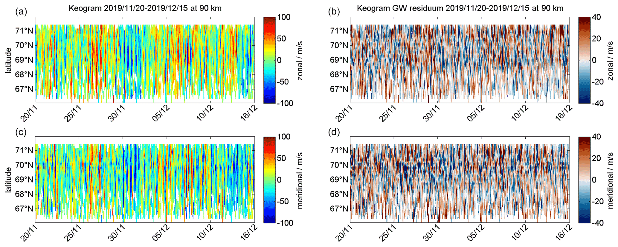
Figure 12The four panels show color-coded latitudinal keograms of zonal and meridional winds for 22∘ longitude and 90 km altitude from 20 November to 15 December 2019.
In Fig. 13, we show an ATW (whole domain) and a keogram for the zonal and meridional wind components that was observed with CONDOR during March 2020. The ATW indicates the presence of a strong diurnal tide during this part of the season, which is also seen in the keogram. the amplitude reaches about 50–60 m s−1 at altitudes in the range from 90–95 km. During this 14 d period, the diurnal tide exhibits some day-to-day variability, similar to what we found at the northern latitudes for the semidiurnal tide. Apparently during the first 8 d of March 2020, the diurnal tide is much weaker compared to the second week. Such a tidal variability seems to be characteristic; however, we did not yet investigate whether a superposition of migrating and non-migrating tides caused this modulation or whether the vertical propagation of the tidal modes was affected in the stratosphere due to gravity waves.
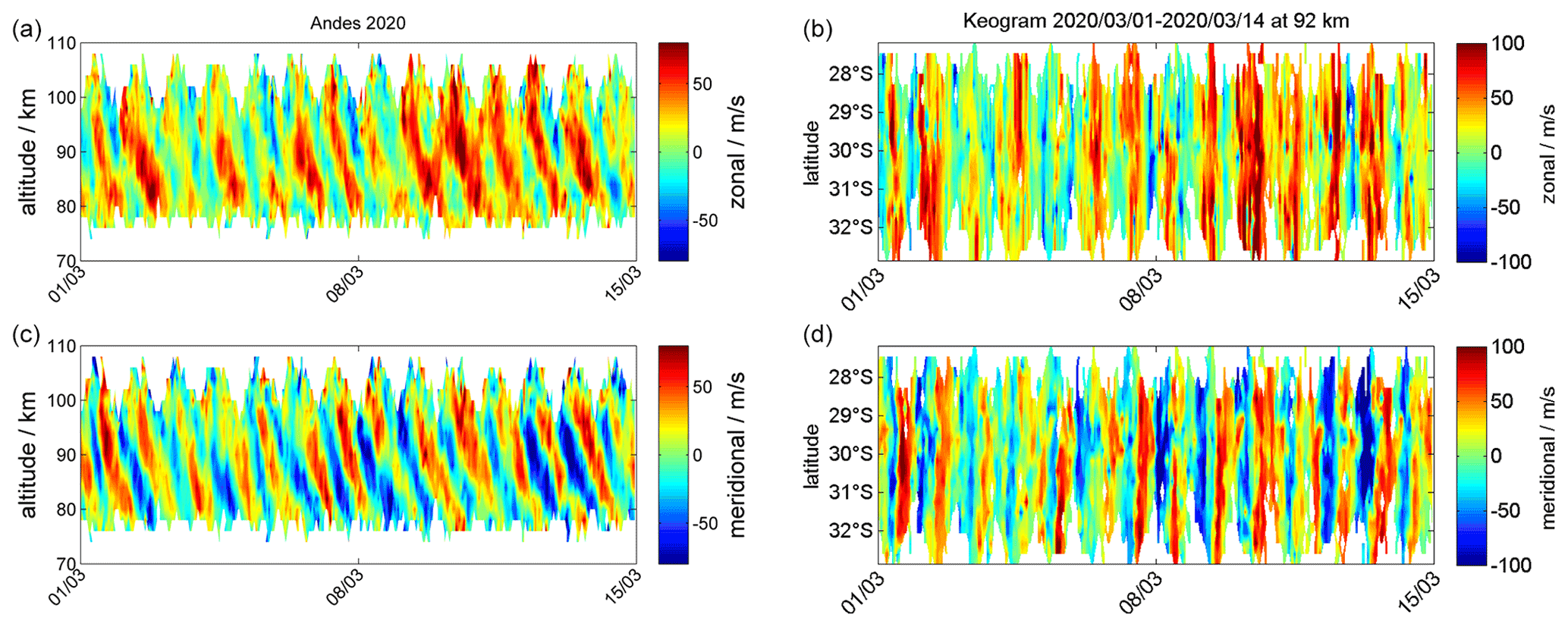
Figure 13The four panels show a ATW measured with CONDOR and the corresponding keogram for the altitude of 92 km. The data were recorded between 1 and 14 March 2020.
4.3 Horizontal wavelength spectra
Another way to investigate the GW activity from the 3D-Var retrievals is to make use of horizontal wavelength spectra, as presented in Stober et al. (2018a). Liu (2019) presents daily zonal wave number zonal wind power spectra derived from Whole Atmosphere Community Circulation Model – Extended at tropospheric and stratospheric altitudes. Nastrom and Gage (1985) estimated kinetic energy spectra from aircraft observations and determined spectral slopes for different wavelength ranges. More recent aircraft observations of horizontal and vertical winds permit us to further investigate the spectral shape for each subrange in more detail but are still limited to the troposphere/lower stratosphere (Schumann, 2019). For horizontal scales between a few kilometers and up to 400–700 km, they derived a spectral slope of , which is often associated with gravity-wave-divergent modes, and a slope of k−3 for the larger scales. However, there is no observational verification of such kinetic energy spectra at the MLT.
Horizontal wavelength spectra are estimated from the 3D-Var retrievals by computing Lomb–Scargle periodograms (Lomb, 1976; Scargle, 1982) of the horizontal wind along all longitudes for each latitude. Thus, we obtain from each image about 20 horizontal wind spectra at a certain altitude, which results in approximately 480 spectra per day. In Fig. 14, we present a typical daily spectrum. The gray points are individual spectral powers from each longitudinal spectra, the thin black line is the daily median spectrum, and the cyan and green lines are slopes for a pre-defined wavelength range that are fitted to the estimated daily median spectrum. The blue and red lines represent spectral slopes corresponding to k−3 and , respectively. We identified a transition scale between the k−3 to the slope at horizontal wavelengths of about 100–120 km. The slopes at the smaller GW scales were more variable, and we found values between k−1.4 and k−1.9 compared to the larger scales. The smallest resolved scales might indicate steeper slopes than expected due to the spatial correlations given by the coupling strength between adjacent grid cells, which tends to suppress small structures by enforcing a certain smoothness. This would imply that the transition between the vortical-driven scales to the divergent GW scale occurs at much smaller wavelengths than in the troposphere. Nastrom and Gage (1985) estimated the transition scale for the troposphere/lower stratosphere to be around 500–700 km.
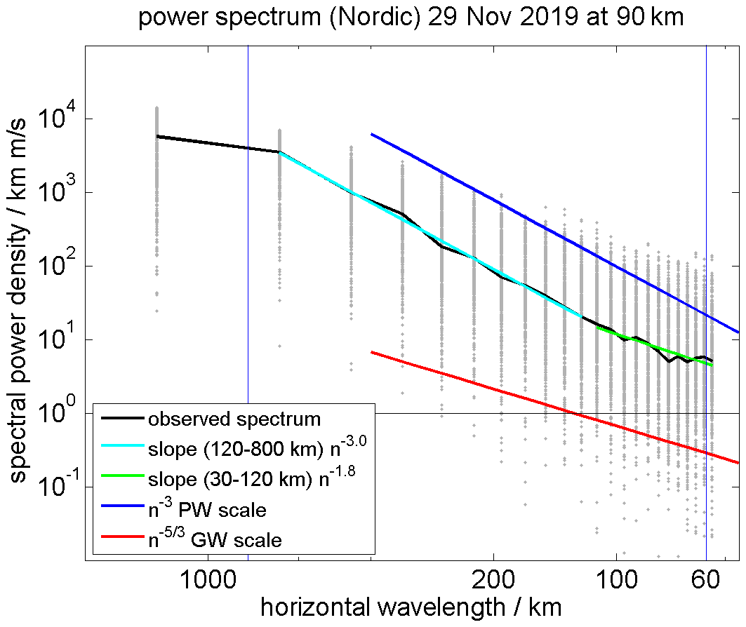
Figure 14Estimated horizontal wavelength spectra for the Nordic Meteor Radar Cluster. The gray points are individual spectral observations, the thin black line is the daily mean spectrum, the cyan and green lines represents fits to the respective wavelengths scale, and the blue and red lines are idealized slopes for planetary waves (PWs) and GWs.
4.4 Residual vertical velocities from 3D-Var
Vertical velocities are also retrieved from the 3D-Var algorithm. However, we are lacking an independent source for validation, and thus we consider them as an additional quality control rather than a geophysical measurement. The measurement responses for the inferred vertical velocities are rather low, implying that this parameter requires larger correlation lengths compared to the horizontal wind components. We use a priori covariances of 5–7 m s−1, and the resultant statistical uncertainties are in the range of 2–4 m s−1, suggesting at least some improvement of a priori covariances by the observations.
The histograms shown in Fig. 15 support at least some statistical interpretation of the variance and median vertical velocity, although the individual values at a certain grid cell may not be useful. These vertical velocity histograms are the result of our forward model and the vertical cost function in the 3D-Var analysis, which forces the vertical velocities to be small by assuming a zero mean value and depend on the choice of our Lagrange multipliers and the a priori covariance. The Lagrange multiplier in the current 3D-Var version is set to 1. The results are obtained using a 4 times stronger vertical weight reflecting the smaller covariance in the vertical velocity cost function, which reduces the oscillations or numerical instabilities. Such numerical instabilities can occur in optimal estimation retrievals and are often related to too-large a priori covariances, which then result in vertical velocities of up to 100 m s−1 and/or variances of about 30–50 m s−1. Thus, the resulting 3D-Var vertical velocity histograms reflect a statistically sound estimate based on our a priori knowledge rather than an entirely independent measurement. Please note that the vertical velocities estimated from the standard retrieval in Fig. 2 are obtained without these assumptions and there is a high degree of consistency between the distributions concerning the small median value of a few cm s−1 and the width of the distribution, which scales with the averaging volume. Hence, the variance is about an order of magnitude larger for the 3D-Var retrieval using 30 km diameter grid cells compared to the monostatic winds, which are based on 300 km diameter volumes.

Figure 15Histograms of the residual vertical velocity bias derived from the 3D-Var retrieval for three successive days and integrated over the full 3-D domain area.
Finally, we demonstrate the applicability of the 3D-Var algorithm to retrieve large-scale wind fields and meteorological wind maps in an area spanning from the Arctic and south to central Norway. Therefore, we expanded the domain of a geographic grid from 61 to 81∘ N and from 6 to 32∘ E. We implemented a 2∘ longitudinal increment and a 0.5∘ increment in latitude. Furthermore, we increased the coupling strength to the next neighbors by a factor of 4. The other settings were similar to those of the retrievals shown above.
This demonstration retrieval was performed with data from December 2012. During this time, a unique configuration of MRs was operational in the Nordic countries and on Svalbard. In addition to the Nordic Meteor Radar Cluster described previously, the Alta MR was in operation on Bear Island (Nozawa et al., 2012), which is located between the Norwegian mainland and Svalbard. The Bear Island radar was located close to the meteorological station on the island (74.475423∘ N, 19.207040∘ E). In addition, this was the first winter season that the Norwegian University of Science and Technology (NTNU) MR at Trondheim (63.406822∘ N, 10.467646∘ E) was operated (de Wit et al., 2014; de Wit et al., 2015). We performed a similar quality control test for the Bear Island and Trondheim MRs as for all other radars and obtained vertical velocity residuals of about 2 cm s−1 and a variance of 15–22 cm s−1 (data not shown). During this period, the Svalbard MR suffered from external interference and detected only 700–800 meteors per day, which resulted in a much lower measurement response.
Figure 16 shows two examples of zonal and meridional winds from the 3D-Var retrieval for December 2012. The wind fields are plotted at all grid cells independent of the width of the averaging kernels, which provides a better visualization of the large-scale flow and the associated high- and low-pressure systems indicated by the wind rotation. Although the wind fields are much smoother compared to the high-resolution retrievals, it is possible to see an increased variability and the presence of smaller-scale dynamics above the radars, in particular, above the Nordic Meteor Radar Cluster consisting of TRO, KIR and SOD at that time. The two snapshots also indicate that there are times with substantially different wind systems above the Arctic latitudes and the Norwegian mainland. There are remarkable differences in the horizontal winds between the two images, although only separated by 2 h in time and 2 km in altitude. This is mainly due to the semidiurnal tide, which is the dominating atmospheric wave during this time of the year at polar latitudes. Climatologies for December show amplitudes between 40–70 m s−1 and vertical wavelengths of about 30–40 km for the semidiurnal tide (Wilhelm et al., 2019; Stober et al., 2020). A semidiurnal tide leads to a clockwise rotation in the flow field, which is found by comparing the wind vectors between the two time steps.
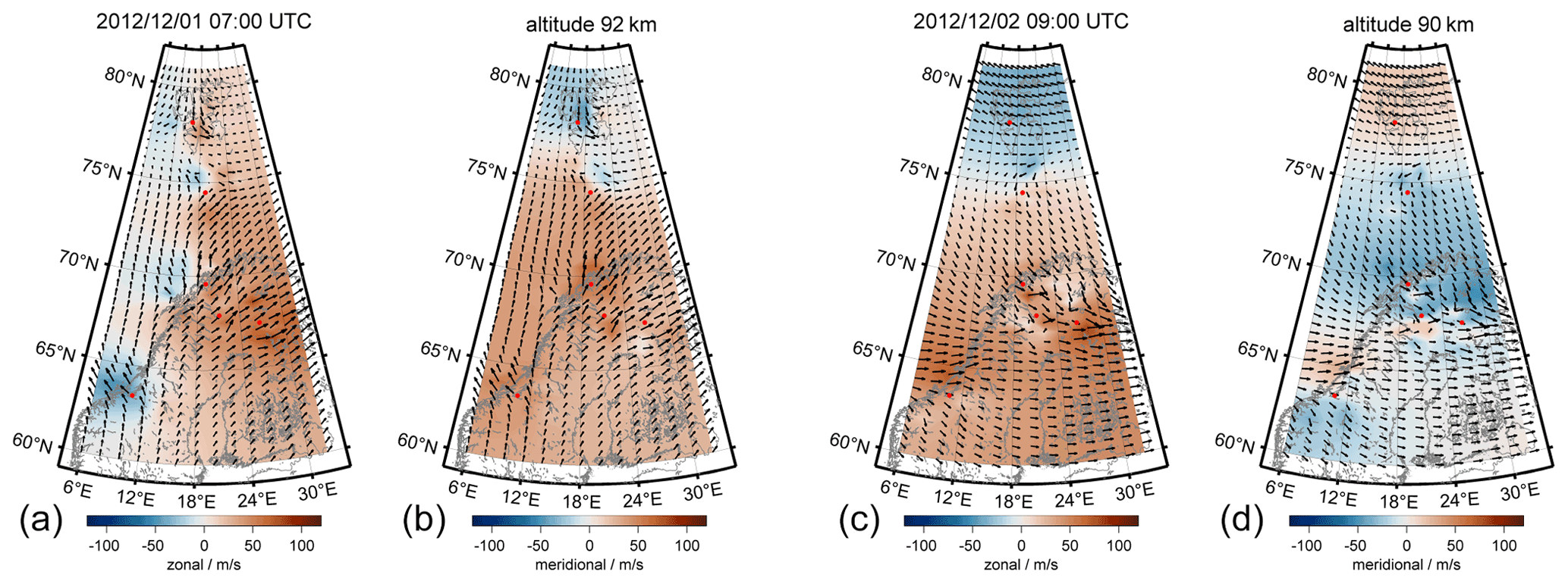
Figure 16Meteorological wind maps obtained from the 3D-Var algorithm using a geographic grid and all MRs involved in ARISE.
When examining the measurement response for such retrievals, shown in Fig. 17, it is straightforward to identify potential locations to improve the network coverage. One objective could be to connect the Trondheim MR to the other Nordic MRs on the mainland. The performed large-scale retrieval made use of meteor radars that contributed to the Atmospheric Dynamics Research InfraStructure in Europe (ARISE) (Blanc et al., 2018). The Bear Island observations support a potential possibility to link the mainland systems up to the Svalbard region by using passive receivers similar to those used for CONDOR.
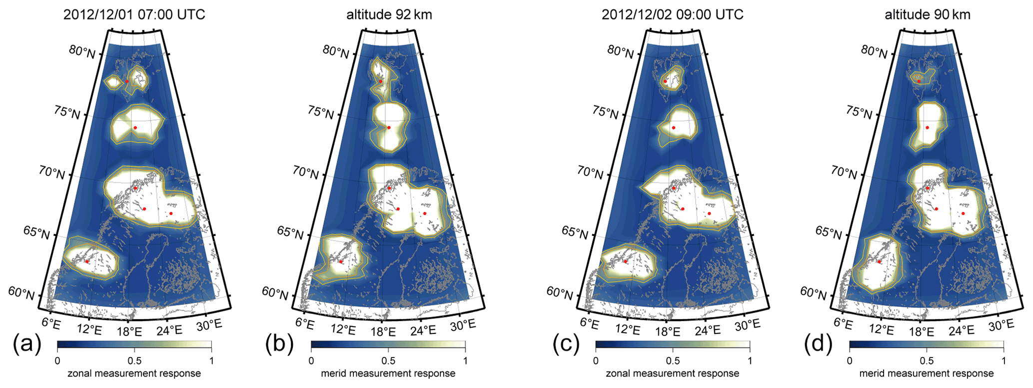
Figure 17Measurement responses for the large-scale retrieval visualized with next-neighbor correlation corresponding to about 120 km resolved scales.
Optimal estimation is an established mathematical technique to retrieve atmospheric quantities and results in statistically sound solutions to inverse problems based on a priori knowledge. During the past years, several multistatic meteor radar networks have been deployed. However, these observations are often analyzed using least squares techniques to infer horizontal inhomogeneities in the wind fields (Stober and Chau, 2015; Chau et al., 2017), which are based on assumptions that are not necessarily valid. Wind speeds in the stratosphere and mesosphere are essentially fast enough to reach the subsonic compressible flow regime (Mach >0.3), and thus terms such as horizontal divergence have to be handled with care.
More recently, initial analyses applying inverse theory were presented by Stober et al. (2018a) and Chau et al. (2021). These retrievals used a Tikhonov regularization to cure the ill-posed mathematical problem by assuming a certain smoothness or curvature and solve for wind vector solutions at pre-defined grid locations or grid cells. Chau et al. (2021) presented some results from a Peruvian meteor radar network using a mean curvature as a constraint for the solution, which in principle is almost identical to the VVP method (Waldteufel and Corbin, 1979), whereas Stober et al. (2018a) only assumed local correlation and retrieved arbitrary wind fields. However, both algorithms just solve the winds within a 2-D layer. The 3D-Var retrieval outlined herein is the first algorithm based on Bayesian statistics and solves the tomographic problem as a full 3-D solution including vertical coupling. The new algorithm is based on the Shannon information entropy (Shannon, 1948) and follows the approaches presented in Rodgers (2000) for the implementation of the optimal estimation.
Another benefit of the 3D-Var retrieval is the possibility to derive the measurement response and the averaging kernels. Both quantities provide essential information about the inverse problem and the reliability of the retrieved quantities and how much information is mixed in from either the a priori distribution or due to remote correlations. We presented some examples of measurement responses for CONDOR and the Nordic Meteor Radar Cluster that apparently indicate that not all wind components can be retrieved within the domains assuming just a next-neighbor correlation with equal reliability reflected by a reduced measurement response. The measurement response for forward scatter systems or multistatic passive links is much less homogeneous compared to monostatic systems. This is understandable in the context of the forward scatter ellipse, which basically results in a large area with a small or almost negligible measurement response for the horizontal winds in the region between the Tx and Rx, whereas the horizontal winds are difficult to retrieve only directly above a monostatic radar. The measurement response for CONDOR contains two separated patches of increased measurement response for the zonal and meridional components, which reflects the alignment of the passive receivers in the north and south directions.
The ASGARD software permits us to use different retrieval grids for the 3D-Var, which can be arbitrarily defined, and use either a Cartesian spacing following the Earth's surface or a geographic grid that is regular in longitude and latitude. This flexibility simplifies potential comparisons to other observations or model outputs for validation. Furthermore, large domains are possible that cover large parts of the globe. Also other data sets can be easily included, even if there is no direct overlap between the observation volumes.
Secondary waves and their resulting forcing on the MLT are an emerging topic (Vadas and Becker, 2018; Vadas et al., 2018). The generation of non-primary waves is driven by large-scale body forces (Vadas and Fritts, 2001). The 3D-Var algorithm is capable of resolving such body forces and the resulting acceleration/deceleration of the mean flow as well as resolving the two counter-rotating vortices. The presented example corresponds to the scales described by Vadas and Fritts (2001) providing confidence in the analysis.
Furthermore, we derived horizontal wavelength spectra similar to those presented in Nastrom and Gage (1985). Our preliminary analysis suggests that the transition between the vortical k−3 and divergent modes occurs at smaller scales compared to those observed in the troposphere. We found a change of the slope at scales around 80–120 km, which is at the edge of the resolution but still at a larger scale than the a priori correlation length.
Finally, we want to mention some additional quality controls that are included in the retrieval. We carefully evaluated all systems for potential range offsets that correspond to altitude deviations between the radars within a network. For the Nordic Meteor Radar Cluster, we performed seasonal analyses and looked for systematic deviations of characteristic seasonal structures such as the summer wind reversal in the zonal wind. A similar attempt was pursued for CONDOR but at a much shorter timescale of 14 d by comparing the vertical diurnal tidal patterns between all systems. The interferometry and alignment of the antennas were validated by estimating the vertical wind biases. Some MRs indicate some skewness in the vertical wind histograms, pointing at some systematic differences. However, all systems observed a residual vertical wind bias on the order of a few cm s−1 (<10 cm s−1) and a standard deviation of 12–30 cm s−1 for the monostatic analysis. The 3D-Var results indicate a much broader distribution but still a very small offset of the mean. Due to the lack of independent validations or other observations, we treat these vertical winds as residual bias. The residual vertical wind bias seems to be in agreement with trace gas observations (Straub et al., 2012) and radar data (Vincent et al., 2019; Gudadze et al., 2019). However, these values show a substantial disagreement to other MR and multistatic MR vertical wind data measurements (Egito et al., 2016; Chau et al., 2021; Conte et al., 2021).
In this study, we present a new 3D-Var retrieval algorithm of the ASGARD software, which is designed to infer 3-D tomographic winds from multistatic observations. The retrieval is applied to two meteor radar networks – CONDOR in Chile in the Andes and the Nordic Meteor Radar Cluster. The 3D-Var retrieval is based on an optimal estimation approach and Bayesian statistics. Thus, the retrieved winds are statistically sound solutions considering the a priori knowledge.
The possibility to perform 3-D tomographic retrievals at the MLT on different geographic or Cartesian grids provides more flexibility for the validation of the obtained winds or to combine and extend the domain areas. Furthermore, the results presented indicate that the algorithm is fast enough to run continuously and still to permit the analysis of small-scale structures. The keogram analysis and the ATW plots are suitable to investigate the large-scale dynamics and to provide a quick overview of the network performance.
The 3D-Var retrievals are capable of resolving counter-rotating vortices that might be related to body forces, which is demonstrated in a case study of a westward-propagating GW above the CONDOR network. The algorithm resolved the two counter-rotating vortices and the acceleration direction of the body force. The spatial scales (horizontal and vertical) for the body force event correspond to the expected theoretical results from previous studies. We were also able to observe large-scale vortices of about 300 km in diameter, which would remain otherwise undiscovered.
Due to the optimal estimation implementation of the 3D-Var, it is possible to compute the measurement response for each time and altitude bin. This information is required to identify potential holes or gaps within existing networks that can be closed by installing additional passive systems or monostatic meteor radars. The measurement response of monostatic radars is optimal to ensure unbiased wind inversion and the most isotropic measurement response. Passive multistatic links are ideally used in combination with monostatic radars. Finally, it is worth considering that passive multistatic links alone show an anisotropic measurement response caused by the shape of the forward scatter ellipse that could lead to biases.
The Appendix includes all geometric coordinate transformations that are used in the paper and are also presented in Stober et al. (2018a). However, we corrected some typos present in the geodetic-to-ECEF coordinate transformation.
A1 Geodetic to ECEF
Radars often are connected to a GPS receiver, which provides the geodetic coordinate in longitude (λ), latitude (ϕ) and height (z). The height refers to the altitude of the radar above the WGS84 reference ellipsoid (National Imagery and Mapping Agency, 2000; Hofmann-Wellenhof et al., 1994). The WGS84 defines the semi-major axis of the Earth to be a=6378137.0 m and a reciprocal of flattening of . The semi-minor axis is given by b=6 356 752.3142 m. These quantities permit us to derive the first eccentricity squared e2, the second eccentricity squared and the radius of Earth's curvature N by
Considering the WGS84 reference ellipsoid of the Earth, any given geodetic location defined by a longitude, latitude and height (above the WGS84 surface) can be transformed to the ECEF coordinates (XR, YR, ZR) by
A2 ECEF to geodetic
The reverse transformation from ECEF to a geodetic longitude (λ), latitude (ϕ) and height (z) is more challenging. Zhu (1993) presents a summary and short validation of several algorithms. The transformation below is based on Heikkinnen (1982). The advantage of this algorithm is the small error and that it is valid from the Earth's center ( km) up to the height of geostationary orbits.
A3 ENU to ECEF
An object observed at a distance R from a known geodetic location in ENU coordinates at a certain azimuth and off-zenith angle can be converted to its ECEF coordinates using the following transformation. Here, the ENU coordinates (xm, ym, zm) are given at a geodetic longitude (λ), latitude (ϕ) and height (z). Rotating the ENU vector (xm, ym, zm) into the ECEF reference (Xm, Ym, Zm) and adding the radar vector results in
A4 ECEF to ENU
The conversion of ECEF to ENU coordinates is given by the line-of-sight vector from the radar towards the meteor in the frame of the ENU coordinates at the geodetic location of the meteor. If the line-of-sight velocity vector is observed at a certain azimuth (az) and zenith (ze) angle relative to the radar, it has a different azimuth az′ and zenith ze′ angle in the frame of the local geodetic coordinates of the meteor. Assuming that we know the ECEF coordinates of the meteor (Xm, Ym, Zm) and the radar location (XR, YR, ZR), it is straightforward to compute the ENU coordinates (x, y, z) by using
The local azimuth az′ and ze′ with respect to the geodetic position of the meteor are obtained by
The data are available upon request. Please contact Alexander Kozlovsky (alexander.kozlovsky@oulu.fi) for the Nordic Meteor Radar Cluster and Alan Liu (LIUZ2@erau.edu) for CONDOR to obtain the 3D-Var retrievals.
GS developed ASGARD and the 3D-Var algorithm. AL, AK and QZ supported the development and implementation of the software at CONDOR and the Nordic Meteor Radar Cluster. JK, EB, CH, MT, SN, PE, RH, NM and ML provided meteor radar data from the networks and supported the implementation of the software. All authors contributed to the editing of the manuscript.
Gunter Stober, Juha Vierinen and Jorge L. Chau submitted a patent on multistatic meteor radar observations using combined pulsed and CW transmitters.
Publisher’s note: Copernicus Publications remains neutral with regard to jurisdictional claims in published maps and institutional affiliations.
Gunter Stober is a member of the Oeschger Center for Climate Change Research (OCCR) at the University of Bern. Most of this software was developed during a sabbatical at the University of Western Ontario. Gunter Stober is grateful to Peter Brown and Robert Sica for the support and discussions during this visit. The authors also want to thank Chris Adami and Ian Reid from ATRAD Ltd., and Brian Fuller and Adrian Murphy from Genesis Ltd. for valuable discussions about some technical aspects of the deployed radars and software. Gunter Stober thanks Andreas Dörnbrack from DLR Oberpfaffenhofen for valuable discussions and helpful comments.
This research has been supported by the STFC (grant no. ST/S000429/1 to Mark Lester) and the Schweizerische Nationalfonds zur Förderung der Wissenschaftlichen Forschung (grant no. 200021_200517/1 to Gunter Stober). The Esrange meteor radar operation, maintenance and data collection were provided by the Esrange Space Center of the Swedish Space Corporation. The 3D-Var retrievals were developed as part of the ARISE design study (http://arise-project.eu/, last access: 8 October 2020) funded by the European Union's Seventh Framework Programme for Research and Technological Development. This work was supported by the Research Council of Norway under the project Svalbard Integrated Arctic Earth Observing System – Infrastructure development of the Norwegian node (SIOS-InfraNor, project no. 269927). This study is partly supported by Grants-in-Aid for Scientific Research (no. 17H02968) of the Japan Society for the Promotion of Science (JSPS).
This paper was edited by Bernd Funke and reviewed by two anonymous referees.
Amante, C. and Eakins, B.: ETOPO1 1 Arc-Minute Global Relief Model, National Geophysical Data Center [data set], https://doi.org/10.7289/V5C8276M, 2009. a
Baumgarten, K. and Stober, G.: On the evaluation of the phase relation between temperature and wind tides based on ground-based measurements and reanalysis data in the middle atmosphere, Ann. Geophys., 37, 581–602, https://doi.org/10.5194/angeo-37-581-2019, 2019. a, b
Baumgarten, K., Gerding, M., and Lübken, F.-J.: Seasonal variation of gravity wave parameters using different filter methods with daylight lidar measurements at midlatitudes, J. Geophys. Res.-Atmos., 122, 2683–2695, https://doi.org/10.1002/2016JD025916, 2017. a
Becker, E.: Dynamical Control of the Middle Atmosphere, Space Sci. Rev., 168, 283–314, https://doi.org/10.1007/s11214-011-9841-5, 2012. a
Becker, E. and Vadas, S. L.: Secondary Gravity Waves in the Winter Mesosphere: Results From a High-Resolution Global Circulation Model, J. Geophys. Res.-Atmos., 123, 2605–2627, https://doi.org/10.1002/2017JD027460, 2018. a, b
Blanc, E., Ceranna, L., Hauchecorne, A., Charlton-Perez, A., Marchetti, E., Evers, L. G., Kvaerna, T., Lastovicka, J., Eliasson, L., Crosby, N. B., Blanc-Benon, P., Le Pichon, A., Brachet, N., Pilger, C., Keckhut, P., Assink, J. D., Smets, P. S. M., Lee, C. F., Kero, J., Sindelarova, T., Kämpfer, N., Rüfenacht, R., Farges, T., Millet, C., Näsholm, S. P., Gibbons, S. J., Espy, P. J., Hibbins, R. E., Heinrich, P., Ripepe, M., Khaykin, S., Mze, N., and Chum, J.: Toward an Improved Representation of Middle Atmospheric Dynamics Thanks to the ARISE Project, Surv. Geophys., 39, 171–225, https://doi.org/10.1007/s10712-017-9444-0, 2018. a
Browning, K. and Wexler, R.: The Determination of Kinematic Properties of a Wind field Using Doppler Radar, J. App. Meteorol., 7, 105–113, 1968. a
Cai, X., Yuan, T., Zhao, Y., Pautet, P.-D., Taylor, M. J., and Pendleton Jr., W. R.: A coordinated investigation of the gravity wave breaking and the associated dynamical instability by a Na lidar and an Advanced Mesosphere Temperature Mapper over Logan, UT (41.7∘ N, 111.8∘ W), J. Geophys. Res.-Space, 119, 6852–6864, https://doi.org/10.1002/2014JA020131, 2014. a
Cao, B., Heale, C. J., Guo, Y., Liu, A. Z., and Snively, J. B.: Observation and modeling of gravity wave propagation through reflection and critical layers above Andes Lidar Observatory at Cerro Pachón, Chile, J. Geophys. Res.-Atmos., 121, 12737–12750, https://doi.org/10.1002/2016JD025173, 2016. a
Chau, J. L., Stober, G., Hall, C. M., Tsutsumi, M., Laskar, F. I., and Hoffmann, P.: Polar mesospheric horizontal divergence and relative vorticity measurements using multiple specular meteor radars, Radio Sci., 52, 811–828, https://doi.org/10.1002/2016RS006225, 2017. a, b, c
Chau, J. L., Urco, J. M., Vierinen, J., Harding, B. J., Clahsen, M., Pfeffer, N., Kuyeng, K. M., Milla, M. A., and Erickson, P. J.: Multistatic Specular Meteor Radar Network in Peru: System Description and Initial Results, Earth Space Sci., 8, e2020EA001293, https://doi.org/10.1029/2020EA001293, 2021. a, b, c, d
Chu, X., Zhao, J., Lu, X., Harvey, V. L., Jones, R. M., Becker, E., Chen, C., Fong, W., Yu, Z., Roberts, B. R., and Dörnbrack, A.: Lidar Observations of Stratospheric Gravity Waves From 2011 to 2015 at McMurdo (77.84∘ S, 166.69∘ E), Antarctica: 2. Potential Energy Densities, Lognormal Distributions, and Seasonal Variations, J. Geophys. Res.-Atmos., 123, 7910–7934, https://doi.org/10.1029/2017JD027386, 2018. a
Conte, J. F., Chau, J. L., Urco, J. M., Latteck, R., Vierinen, J., and Salvador, J. O.: First Studies of Mesosphere and Lower Thermosphere Dynamics Using a Multistatic Specular Meteor Radar Network Over Southern Patagonia, Earth Space Sci., 8, e2020EA001356, https://doi.org/10.1029/2020EA001356, 2021. a, b
de Wit, R., Hibbins, R., and Espy, P.: The seasonal cycle of gravity wave momentum flux and forcing in the high latitude northern hemisphere mesopause region, J. Atmos. Sol.-Terr. Phy., 127, 21–29, https://doi.org/10.1016/j.jastp.2014.10.002, 2015. a
de Wit, R. J., Hibbins, R. E., Espy, P. J., Orsolini, Y. J., Limpasuvan, V., and Kinnison, D. E.: Observations of gravity wave forcing of the mesopause region during the January 2013 major Sudden Stratospheric Warming, Geophys. Res. Lett., 41, 4745–4752, https://doi.org/10.1002/2014GL060501, 2014. a
de Wit, R. J., Janches, D., Fritts, D. C., Stockwell, R. G., and Coy, L.: Unexpected climatological behavior of MLT gravity wave momentum flux in the lee of the Southern Andes hot spot, Geophys. Res. Lett., 44, 1182–1191, https://doi.org/10.1002/2016GL072311, 2017. a
Dempsey, S. M., Hindley, N. P., Moffat-Griffin, T., Wright, C. J., Smith, A. K., Du, J., and Mitchell, N. J.: Winds and tides of the Antarctic mesosphere and lower thermosphere: One year of meteor-radar observations over Rothera (68∘ S, 68∘ W) and comparisons with WACCM and eCMAM, J. Atmos. Sol.-Terr. Phy., 212, 105510, https://doi.org/10.1016/j.jastp.2020.105510, 2021. a, b, c
Egito, F., Andrioli, V., and Batista, P.: Vertical winds and momentum fluxes due to equatorial planetary scale waves using all-sky meteor radar over Brazilian region, J. Atmos. Sol.-Terr. Phy., 149, 108–119, https://doi.org/10.1016/j.jastp.2016.10.005, 2016. a, b
Ehard, B., Kaifler, B., Kaifler, N., and Rapp, M.: Evaluation of methods for gravity wave extraction from middle-atmospheric lidar temperature measurements, Atmos. Meas. Tech., 8, 4645–4655, https://doi.org/10.5194/amt-8-4645-2015, 2015. a
Ern, M., Preusse, P., Gille, J. C., Hepplewhite, C. L., Mlynczak, M. G., Russell III, J. M., and Riese, M.: Implications for atmospheric dynamics derived from global observations of gravity wave momentum flux in stratosphere and mesosphere, J. Geophys. Res., 116, D19107, https://doi.org/10.1029/2011JD015821, 2011. a, b
Ern, M., Hoffmann, L., and Preusse, P.: Directional gravity wave momentum fluxes in the stratosphere derived from high-resolution AIRS temperature data, Geophys. Res. Lett., 44, 475–485, https://doi.org/10.1002/2016GL072007, 2017. a
Fritts, D. and Alexander, M. J.: Gravity wave dynamics and effects in the middle atmosphere, Rev. Geophys., 41, 1–64, https://doi.org/10.1029/2001RG000106, 2003. a
Fritts, D. C., Vadas, S. L., and Yamada, Y.: An estimate of strong local body forcing and gravity wave radiation based on OH airglow and meteor radar observations, Geophys. Res. Lett., 29, 71-1–71-4, https://doi.org/10.1029/2001GL013753, 2002. a
Fritts, D. C., Janches, D., Iimura, H., Hocking, W. K., Mitchell, N. J., Stockwell, R. G., Fuller, B., Vandepeer, B., Hormaechea, J., Brunini, C., and Levato, H.: Southern Argentina Agile Meteor Radar: System design and initial measurements of large-scale winds and tides, J. Geophys. Res., 115, D18112, https://doi.org/10.1029/2010JD013850, 2010. a
Geller, M. A., Alexander, M. J., Love, P. T., Bacmeister, J., Ern, M., Hertzog, A., Manzini, E., Preusse, P., Sato, K., Scaife, A. A., and Zhou, T.: A Comparison between Gravity Wave Momentum Fluxes in Observations and Climate Models, J. Climate, 26, 6383–6405, https://doi.org/10.1175/JCLI-D-12-00545.1, 2013. a
Gudadze, N., Stober, G., and Chau, J. L.: Can VHF radars at polar latitudes measure mean vertical winds in the presence of PMSE?, Atmos. Chem. Phys., 19, 4485–4497, https://doi.org/10.5194/acp-19-4485-2019, 2019. a, b, c
Hagen, J., Murk, A., Rüfenacht, R., Khaykin, S., Hauchecorne, A., and Kämpfer, N.: WIRA-C: a compact 142-GHz-radiometer for continuous middle-atmospheric wind measurements, Atmos. Meas. Tech., 11, 5007–5024, https://doi.org/10.5194/amt-11-5007-2018, 2018. a, b, c
Harding, B. J., Makela, J. J., and Meriwether, J. W.: Estimation of mesoscale thermospheric wind structure using a network of interferometers, J. Geophys. Res.-Space, 120, 3928–3940, https://doi.org/10.1002/2015JA021025, 2015. a
Hauchecorne, A. and Chanin, M. L.: Density and Temperature Profiles obtained by Lidar between 35 and 70 km, Geophys. Res. Lett., 7, 565–568, 1980. a
Heale, C. J., Bossert, K., Vadas, S. L., Hoffmann, L., Dörnbrack, A., Stober, G., Snively, J. B., and Jacobi, C.: Secondary Gravity Waves Generated by Breaking Mountain Waves Over Europe, J. Geophys. Res.-Atmos., 125, e2019JD031662, https://doi.org/10.1029/2019JD031662, 2020. a
Hecht, J. H., Wan, K., Gelinas, L. J., Fritts, D. C., Walterscheid, R. L., Rudy, R. J., Liu, A. Z., Franke, S. J., Vargas, F. A., Pautet, P. D., Taylor, M. J., and Swenson, G. R.: The life cycle of instability features measured from the Andes Lidar Observatory over Cerro Pachon on 24 March 2012, J. Geophys. Res.-Atmos., 119, 8872–8898, https://doi.org/10.1002/2014JD021726, 2014. a, b
Hecht, J. H., Fritts, D. C., Wang, L., Gelinas, L. J., Rudy, R. J., Walterscheid, R. L., Taylor, M. J., Pautet, P. D., Smith, S., and Franke, S. J.: Observations of the Breakdown of Mountain Waves Over the Andes Lidar Observatory at Cerro Pachon on 8/9 July 2012, J. Geophys. Res.-Atmos., 123, 276–299, https://doi.org/10.1002/2017JD027303, 2018. a
Heikkinnen, M.: Geschlossene Formeln zur Berechnung räumlicher geodätischer Koordinaten aus rechtwinkligen Koordinaten, Z. Ermess., 107, 207–2011, 1982. a, b
Hocking, W., Fuller, B., and Vandepeer, B.: Real-time determination of meteor-related parameters utilizing modern digital technology, J. Atmos. Sol.-Terr. Phy., 63, 155–169, https://doi.org/10.1016/S1364-6826(00)00138-3, 2001. a, b, c, d, e, f, g
Hocking, W. K.: Temperatures Using radar-meteor decay times, Geophys. Res. Lett., 26, 3297–3300, https://doi.org/10.1029/1999GL003618, 1999. a
Hoffmann, P., Singer, W., Keuer, D., Hocking, W., Kunze, M., and Murayama, Y.: Latitudinal and longitudinal variability of mesospheric winds and temperatures during stratospheric warming events, J. Atmos. Sol.-Terr. Phy., 69, 2355–2366, https://doi.org/10.1016/j.jastp.2007.06.010, 2007. a
Hofmann-Wellenhof, B., Lichtenegger, H., and Collins, J.: Global Positioning System: theory and practice, Springer-Verlag, 1994. a
Holdsworth, D. A., Reid, I. M., and Cervera, M. A.: Buckland Park all-sky interferometric meteor radar, Radio Sci., 39, RS5009, https://doi.org/10.1029/2003RS003014, 2004. a, b, c, d
Jacobs, E. and Ralston, E. W.: Ambiguity Resolution in Interferometry, IEEE T. Aero. Elec. Sys., AES-17, 766–780, 1981. a
Jones, J., Webster, A. R., and Hocking, W. K.: An improved interferometer design for use with meteor radars, Radio Sci., 33, 55–65, https://doi.org/10.1029/97RS03050, 1998. a
Krueger, D. A., She, C.-Y., and Yuan, T.: Retrieving mesopause temperature and line-of-sight wind from full-diurnal-cycle Na lidar observations, Appl. Optics, 54, 9469–9489, https://doi.org/10.1364/AO.54.009469, 2015. a
Lange, M. and Jacobi, C.: Analysis of Gravity Waves from Radio Occultation Measurements, Springer Berlin Heidelberg, Berlin, Heidelberg, 479–484, https://doi.org/10.1007/978-3-540-38366-6_65, 2003. a
Larsen, M., Fukao, S., Aruga, O., Yamanaka, M., Tsuda, T., and Kato, S.: A Comparison of VHF Radar Vertical-Velocity Measurements by a Direct Vertical-Beam Method and by a VAD Technique, J. Atmos. Ocean. Tech., 8, 766–776, 1991. a
Latteck, R., Singer, W., Rapp, M., Vandepeer, B., Renkwitz, T., Zecha, M., and Stober, G.: MAARSY: The new MST radar on Andøya–System description and first results, Radio Sci., 47, RS1006, https://doi.org/10.1029/2011RS004775, 2012. a
Lindzen, R. S.: Turbulence and stress owing to gravity wave and tidal breakdown, J. Geophys. Res., 86, 9707–9714, https://doi.org/10.1029/JC086iC10p09707, 1981. a
Liu, H.-L.: Quantifying gravity wave forcing using scale invariance, Nat. Commun., 10, 2605, https://doi.org/10.1038/s41467-019-10527-z, 2019. a
Livesey, N. J., Van Snyder, W., Read, W. G., and Wagner, P. A.: Retrieval algorithms for the EOS Microwave limb sounder (MLS), IEEE T. Geosci. Remote, 44, 1144–1155, 2006. a, b, c
Lomb, N. R.: Least-squares frequency analysis of unequally spaced data, Astrophys. Space Sci., 39, 447–462, https://doi.org/10.1007/BF00648343, 1976. a
Nastrom, G. and Gage, K.: A Climatology of Atmospheric Wavenumber Spectra of Wind and Temperature Observed by Commercial Aircraft, J. Atmos. Sci., 42, 950–960, https://doi.org/10.1175/1520-0469(1985)042<0950:ACOAWS>2.0.CO;2, 1985. a, b, c
National Imagery and Mapping Agency: Department of Defense World Geodetic System 1984: its definition and relationships with local geodetic systems, National Imagery and Mapping Agency, St. Louis, MO, USA, Tech. Rep. TR8350.2, available at: https://apps.dtic.mil/sti/pdfs/ADA280358.pdf (last access: 28 September 2021), 2000. a, b
Navas-Guzmán, F., Kämpfer, N., and Haefele, A.: Validation of brightness and physical temperature from two scanning microwave radiometers in the 60 GHz O2 band using radiosonde measurements, Atmos. Meas. Tech., 9, 4587–4600, https://doi.org/10.5194/amt-9-4587-2016, 2016. a
Nozawa, S., Hall, C., Tsutsumi, M., Brekke, A., Ogawa, Y., Tsuda, T., Oyama, S., and Fujii, R.: Mean winds, tides, and quasi-2 day waves above Bear Island, J. Atmos. Sol.-Terr. Phy., 90-91, 26–44, https://doi.org/10.1016/j.jastp.2012.05.002, 2012. a
Pancheva, D., Mukhtarov, P., Hall, C., Meek, C., Tsutsumi, M., Pedatella, N., Nozawa, S., and Manson, A.: Climatology of the main (24-h and 12-h) tides observed by meteor radars at Svalbard and Tromsø: Comparison with the models CMAM-DAS and WACCM-X, J. Atmos. Sol.-Terr. Phy., 207, 105339, https://doi.org/10.1016/j.jastp.2020.105339, 2020. a
Pautet, P.-D., Taylor, M. J., Fritts, D. C., Bossert, K., Williams, B. P., Broutman, D., Ma, J., Eckermann, S. D., and Doyle, J. D.: Large-amplitude mesospheric response to an orographic wave generated over the Southern Ocean Auckland Islands (50.7∘ S) during the DEEPWAVE project, J. Geophys. Res.-Atmos., 121, 1431–1441, https://doi.org/10.1002/2015JD024336, 2016. a
Pautet, P.-D., Taylor, M. J., Eckermann, S. D., and Criddle, N.: Regional Distribution of Mesospheric Small-Scale Gravity Waves During DEEPWAVE, J. Geophys. Res.-Atmos., 124, 7069–7081, https://doi.org/10.1029/2019JD030271, 2019. a
Pautet, P.-D., Taylor, M. J., Fritts, D. C., Janches, D., Kaifler, N., Dörnbrack, A., and Hormaechea, J. L.: Mesospheric Mountain Wave Activity in the Lee of the Southern Andes, J. Geophys. Res.-Atmos., 126, e2020JD033268, https://doi.org/10.1029/2020JD033268, 2021. a
Plougonven, R. and Zhang, F.: Internal gravity waves from atmospheric jets and fronts, Rev. Geophys., 52, 33–76, https://doi.org/10.1002/2012RG000419, 2014. a
Preusse, P., Dörnbrack, A., Eckermann, S. D., Riese, M., Schaeler, B., Bacmeister, J. T., Broutman, D., and Grossmann, K. U.: Space-based measurements of stratospheric mountain waves by CRISTA 1. Sensitivity, analysis method, and a case study, J. Geophys. Res., 107, 8178, https://doi.org/10.1029/2001JD000699, 2002. a
Randall, C. E., Carstens, J., France, J. A., Harvey, V. L., Hoffmann, L., Bailey, S. M., Alexander, M. J., Lumpe, J. D., Yue, J., Thurairajah, B., Siskind, D. E., Zhao, Y., Taylor, M. J., and Russell III, J. M.: New AIM/CIPS global observations of gravity waves near 50–55 km, Geophys. Res. Lett., 44, 7044–7052, https://doi.org/10.1002/2017GL073943, 2017. a
Rodgers, C. D.: Inverse Methods for Atmospheric Sounding: Theory and Practice, World Scientific, Singapore, ISBN 981-02-2740-X, 2000. a, b, c, d
Rüfenacht, R., Baumgarten, G., Hildebrand, J., Schranz, F., Matthias, V., Stober, G., Lübken, F.-J., and Kämpfer, N.: Intercomparison of middle-atmospheric wind in observations and models, Atmos. Meas. Tech., 11, 1971–1987, https://doi.org/10.5194/amt-11-1971-2018, 2018. a
Scargle, J. D.: Studies in astronomical time series analysis. II – Statistical aspects of spectral analysis of unevenly spaced data, Astrophys. J., 263, 835–853, 1982. a
Schranz, F., Hagen, J., Stober, G., Hocke, K., Murk, A., and Kämpfer, N.: Small-scale variability of stratospheric ozone during the sudden tratospheric warming 2018/2019 observed at Ny-Ålesund, Svalbard, Atmos. Chem. Phys., 20, 10791–10806, https://doi.org/10.5194/acp-20-10791-2020, 2020. a
Schumann, U.: The Horizontal Spectrum of Vertical Velocities near the Tropopause from Global to Gravity Wave Scales, J. Atmos. Sci., 76, 3847–3862, https://doi.org/10.1175/JAS-D-19-0160.1, 2019. a
Schwartz, M., Lambert, A., Manney, G., Read, W., Livesey, N., Froidevaux, L., Ao, C., Bernath, P., Boone, C., Cofield, R., Daffer, W., Drouin, B., Fetzer, E., Fuller, R., Jarnot, R., Jiang, J., Jiang, Y., Knosp, B. W., Krüger, K., Li, J.-L., Mlynczak, M., Pawson, S., Russell, J., Santee, M., Snyder, W., Stek, P., Thurstans, R., Tompkins, A., Wagner, P., Walker, K., Waters, J. W., and Wu, D. L.: Validation of the Aura Microwave Limb Sounder temperature and geopotential height measurements, J. Geophys. Res., 113, D15S11, https://doi.org/10.1029/2007JD008783, 2008. a, b, c
Shannon, C. E.: A Mathematical Theory of Communication, Bell Syst. Tech. J., 27, 379–423, https://doi.org/10.1002/j.1538-7305.1948.tb01338.x, 1948. a
Shannon, C. E. and Weaver, W.: The Mathematical Theory of Communication, University of Illinois Press, Urbana, IL, 1949. a
Sica, R. J. and Haefele, A.: Retrieval of temperature from a multiple-channel Rayleigh-scatter lidar using an optimal estimation method, Appl. Optics, 54, 1872–1889, https://doi.org/10.1364/AO.54.001872, 2015. a
Smith, S. M.: The identification of mesospheric frontal gravity-wave events at a mid-latitude site, Adv. Space Res., 54, 417–424, https://doi.org/10.1016/j.asr.2013.08.014, 2014. a
Spargo, A. J., Reid, I. M., and MacKinnon, A. D.: Multistatic meteor radar observations of gravity-wave–tidal interaction over southern Australia, Atmos. Meas. Tech., 12, 4791–4812, https://doi.org/10.5194/amt-12-4791-2019, 2019. a, b
Stober, G.: Remote sensing of Middle Atmospheric Dynamics at mid- and polar latitudes, habilitation, University Bern, 2020. a
Stober, G. and Chau, J. L.: A multistatic and multifrequency novel approach for specular meteor radars to improve wind measurements in the MLT region, Radio Sci., 50, 431–442, https://doi.org/10.1002/2014RS005591, 2015. a, b, c
Stober, G., Sommer, S., Rapp, M., and Latteck, R.: Investigation of gravity waves using horizontally resolved radial velocity measurements, Atmos. Meas. Tech., 6, 2893–2905, https://doi.org/10.5194/amt-6-2893-2013, 2013. a
Stober, G., Matthias, V., Jacobi, C., Wilhelm, S., Höffner, J., and Chau, J. L.: Exceptionally strong summer-like zonal wind reversal in the upper mesosphere during winter 2015/16, Ann. Geophys., 35, 711–720, https://doi.org/10.5194/angeo-35-711-2017, 2017. a, b
Stober, G., Chau, J. L., Vierinen, J., Jacobi, C., and Wilhelm, S.: Retrieving horizontally resolved wind fields using multi-static meteor radar observations, Atmos. Meas. Tech., 11, 4891–4907, https://doi.org/10.5194/amt-11-4891-2018, 2018a. a, b, c, d, e, f, g, h, i, j, k, l, m, n
Stober, G., Sommer, S., Schult, C., Latteck, R., and Chau, J. L.: Observation of Kelvin–Helmholtz instabilities and gravity waves in the summer mesopause above Andenes in Northern Norway, Atmos. Chem. Phys., 18, 6721–6732, https://doi.org/10.5194/acp-18-6721-2018, 2018b. a
Stober, G., Baumgarten, K., McCormack, J. P., Brown, P., and Czarnecki, J.: Comparative study between ground-based observations and NAVGEM-HA analysis data in the mesosphere and lower thermosphere region, Atmos. Chem. Phys., 20, 11979–12010, https://doi.org/10.5194/acp-20-11979-2020, 2020. a, b, c
Stober, G., Janches, D., Matthias, V., Fritts, D., Marino, J., Moffat-Griffin, T., Baumgarten, K., Lee, W., Murphy, D., Kim, Y. H., Mitchell, N., and Palo, S.: Seasonal evolution of winds, atmospheric tides, and Reynolds stress components in the Southern Hemisphere mesosphere–lower thermosphere in 2019, Ann. Geophys., 39, 1–29, https://doi.org/10.5194/angeo-39-1-2021, 2021. a, b, c, d
Straub, C., Tschanz, B., Hocke, K., Kämpfer, N., and Smith, A. K.: Transport of mesospheric H2O during and after the stratospheric sudden warming of January 2010: observation and simulation, Atmos. Chem. Phys., 12, 5413–5427, https://doi.org/10.5194/acp-12-5413-2012, 2012. a
Stähli, O., Murk, A., Kämpfer, N., Mätzler, C., and Eriksson, P.: Microwave radiometer to retrieve temperature profiles from the surface to the stratopause, Atmos. Meas. Tech., 6, 2477–2494, https://doi.org/10.5194/amt-6-2477-2013, 2013. a, b
Takahashi, T., Nozawa, S., Tsuda, T. T., Ogawa, Y., Saito, N., Hidemori, T., Kawahara, T. D., Hall, C., Fujiwara, H., Matuura, N., Brekke, A., Tsutsumi, M., Wada, S., Kawabata, T., Oyama, S., and Fujii, R.: A case study on generation mechanisms of a sporadic sodium layer above Tromsø (69.6∘ N) during a night of high auroral activity, Ann. Geophys., 33, 941–953, https://doi.org/10.5194/angeo-33-941-2015, 2015. a
Taylor, M. J., Pendleton, W. R., Clark, S., Takahashi, H., Gobbi, D., and Goldberg, R. A.: Image measurements of short-period gravity waves at equatorial latitudes, J. Geophys. Res., 102, 26283–26299, https://doi.org/10.1029/96JD03515, 1997. a
Trinh, Q. T., Kalisch, S., Preusse, P., Chun, H.-Y., Eckermann, S. D., Ern, M., and Riese, M.: A comprehensive observational filter for satellite infrared limb sounding of gravity waves, Atmos. Meas. Tech., 8, 1491–1517, https://doi.org/10.5194/amt-8-1491-2015, 2015. a
Trinh, Q. T., Ern, M., Doornbos, E., Preusse, P., and Riese, M.: Satellite observations of middle atmosphere–thermosphere vertical coupling by gravity waves, Ann. Geophys., 36, 425–444, https://doi.org/10.5194/angeo-36-425-2018, 2018. a
Vadas, S. L. and Becker, E.: Numerical Modeling of the Excitation, Propagation, and Dissipation of Primary and Secondary Gravity Waves during Wintertime at McMurdo Station in the Antarctic, J. Geophys. Res.-Atmos., 123, 9326–9369, https://doi.org/10.1029/2017JD027974, 2018. a, b, c
Vadas, S. L. and Fritts, D. C.: Gravity Wave Radiation and Mean Responses to Local Body Forces in the Atmosphere, J. Atmos. Sci., 58, 2249–2279, https://doi.org/10.1175/1520-0469(2001)058<2249:GWRAMR>2.0.CO;2, 2001. a, b, c, d
Vadas, S. L., Zhao, J., Chu, X., and Becker, E.: The Excitation of Secondary Gravity Waves From Local Body Forces: Theory and Observation, J. Geophys. Res.-Atmos., 123, 9296–9325, https://doi.org/10.1029/2017JD027970, 2018. a, b
Vincent, R. A., Kovalam, S., Murphy, D. J., Reid, I. M., and Younger, J. P.: Trends and Variability in Vertical Winds in the Southern Hemisphere Summer Polar Mesosphere and Lower Thermosphere, J. Geophys. Res.-Atmos., 124, 11070–11085, https://doi.org/10.1029/2019JD030735, 2019. a
Waldteufel, P. and Corbin, H.: On the Analysis of Single-Doppler Radar Data, J. Appl. Meteorol. Clim., 18, 532–542, https://doi.org/10.1175/1520-0450(1979)018<0532:OTAOSD>2.0.CO;2, 1979. a, b
Wilhelm, S., Stober, G., and Chau, J. L.: A comparison of 11-year mesospheric and lower thermospheric winds determined by meteor and MF radar at 69∘ N, Ann. Geophys., 35, 893–906, https://doi.org/10.5194/angeo-35-893-2017, 2017. a
Wilhelm, S., Stober, G., and Brown, P.: Climatologies and long-term changes in mesospheric wind and wave measurements based on radar observations at high and mid latitudes, Ann. Geophys., 37, 851–875, https://doi.org/10.5194/angeo-37-851-2019, 2019. a
Wörl, R., Strelnikov, B., Viehl, T. P., Höffner, J., Pautet, P.-D., Taylor, M. J., Zhao, Y., and Lübken, F.-J.: Thermal structure of the mesopause region during the WADIS-2 rocket campaign, Atmos. Chem. Phys., 19, 77–88, https://doi.org/10.5194/acp-19-77-2019, 2019. a
Wu, Q., Killeen, T., Ortland, D., Solomon, S., Gablehouse, R., Johnson, R., Skinner, W., Niciejewski, R., and Franke, S.: TIMED Doppler interferometer (TIDI) observations of migrating diurnal and semidiurnal tides, J. Atmos. Sol.-Terr. Phy., 68, 408–417, https://doi.org/10.1016/j.jastp.2005.02.031, 2006. a
Yuan, T., Heale, C. J., Snively, J. B., Cai, X., Pautet, P.-D., Fish, C., Zhao, Y., Taylor, M. J., Pendleton Jr., W. R., Wickwar, V., and Mitchell, N. J.: Evidence of dispersion and refraction of a spectrally broad gravity wave packet in the mesopause region observed by the Na lidar and Mesospheric Temperature Mapper above Logan, Utah, J. Geophys. Res.-Atmos., 121, 579–594, https://doi.org/10.1002/2015JD023685, 2016. a
Zhu, J.: Exact conversion of earth-centered, earth-fixed coordinates to geodetic coordinates, J. Guid. Control Dynam., 16, 389–391, 1993. a, b
- Abstract
- Introduction
- Nordic Meteor Radar Cluster and CONDOR
- Atmospheric tomography – 3D-Var retrieval
- Scientific results
- Large-scale retrievals – meteorological wind maps
- Discussion
- Conclusions
- Appendix A: Coordinate transformations
- Data availability
- Author contributions
- Competing interests
- Disclaimer
- Acknowledgements
- Financial support
- Review statement
- References