the Creative Commons Attribution 4.0 License.
the Creative Commons Attribution 4.0 License.
 | 11 Oct 2021
Correcting bias in log-linear instrument calibrations in the context of chemical ionization mass spectrometry
Chenyang Bi
Jordan E. Krechmer
Manjula R. Canagaratna
Quantitative calibration of analytes using chemical ionization mass spectrometers (CIMSs) has been hindered by the lack of commercially available standards of atmospheric oxidation products. To accurately calibrate analytes without standards, techniques have been recently developed to log-linearly correlate analyte sensitivity with instrument operating conditions. However, there is an inherent bias when applying log-linear calibration relationships that is typically ignored. In this study, we examine the bias in a log-linear-based calibration curve based on prior mathematical work. We quantify the potential bias within the context of a CIMS-relevant relationship between analyte sensitivity and instrument voltage differentials. Uncertainty in three parameters has the potential to contribute to the bias, specifically the inherent extent to which the nominal relationship can capture true sensitivity, the slope of the relationship, and the voltage differential below which maximum sensitivity is achieved. Using a prior published case study, we estimate an average bias of 30 %, with 1 order of magnitude for less sensitive compounds in some circumstances. A parameter-explicit solution is proposed in this work for completely removing the inherent bias generated in the log-linear calibration relationships. A simplified correction method is also suggested for cases where a comprehensive bias correction is not possible due to unknown uncertainties of calibration parameters, which is shown to eliminate the bias on average but not for each individual compound.
- Article
(3273 KB) - Full-text XML
-
Supplement
(1063 KB) - BibTeX
- EndNote


The time-of-flight chemical ionization mass spectrometer (Tof-CIMS) has been widely used for online characterization of organic compounds in the atmosphere. Gas-phase analytes are reacted with reagent ions to form analyte ions and then detected and classified by mass spectrometry. Many reagent ions have been examined, with some of the most popular being hydronium (Yuan et al., 2016; Lindinger et al., 1998), acetate (Bertram et al., 2011; Brophy and Farmer, 2016), nitrate (Jokinen et al., 2012; Krechmer et al., 2015), CF3O (Crounse et al., 2006; St Clair et al., 2010), and iodide (Lee et al., 2014; Slusher, 2004). Each reagent ion accesses a different region of chemical space (Riva et al., 2019; Isaacman-Vanwertz et al., 2017) and differs in its range of sensitivities, from relatively universal to highly variable. For example, proton transfer reaction is commonly used for measurements of less oxidized compounds with a sensitivity that varies only by a factor of up to 3 or 4 for most analytes (Sekimoto et al., 2017). In contrast, iodide is most useful for semivolatile, oxidized compounds, but sensitivity varies by several orders of magnitude (Iyer et al., 2016; Lopez-Hilfiker et al., 2016).
Unfortunately, these wide ranges in sensitivity pose significant issues in the quantitative measurement of ambient atmospheres. For many atmospheric constituents, it is not possible or not feasible to calibrate using authentic standards, due to a lack of commercial availability and/or chemical instability (thermal lability, flammability, etc.) (Brophy, 2016). Several approaches have consequently been developed to estimate the sensitivity of a CIMS instrument to a given analyte based on either its physicochemical properties (e.g., dipole moment and polarizability) (Sekimoto et al., 2017) or its observed response (e.g., induced dissociation) to changing instrument conditions (Zaytsev et al., 2019; Lopez-Hilfiker et al., 2016). Estimating instrument sensitivity based on derived relationships between sensitivity and other properties inherently carries some uncertainty, as the relationship is unlikely to be ideal and typically includes some scatters. Nevertheless, this approach of “derived sensitivity” is often the best (or only) tool available for calibration, so a close look is warranted into the implications of this approach for the error of a single analyte, as well as the combined error of the sum of many analytes.
Previous work, which we discuss in detail in the following section, has examined the uncertainty in estimating a parameter from a derived relationship (i.e., using a regression model to predict a value). Specifically, prediction of a value (e.g., sensitivity) from a linear model introduces no bias and has normally distributed error, but in more complex relationships (involving log-transformations, step functions, etc.), bias and other errors may be introduced. Many of the derived sensitivity relationships used for CIMS have more complex forms, so the overarching goal of this work is to evaluate and correct for biases and other errors in the types of relationships used for estimating CIMS sensitivities.
We focus in this work on the calibrations of analytes in an iodide CIMS because (1) this measurement technique is widely used, (2) it has orders of magnitude variance in sensitivities (Iyer et al., 2016), and (3) estimating its sensitivity often relies on a complex (log-linear, piece-wise) sensitivity relationship. Iyer et al. (2016) have shown that the sensitivities of analytes in an iodide CIMS are log-linearly correlated with the binding enthalpy of the iodide-analyte adduct, with some maximum sensitivity that is limited by the rate of collisions between the analyte and the reagent ion. Lopez-Hilfiker et al. (2016) further suggested that modulating voltage differences in certain components of the mass spectrometer (i.e., between the skimmer of the small-segmented quadrupole and the entrance of the big-segmented quadrupole) can introduce de-clustering of the iodide-molecule adduct. The parameter, dV50, which is the voltage difference where signals of a compound are at half-maximum, is reported to be an indicator of the binding enthalpy of the adduct (Lopez-Hilfiker et al., 2016; Iyer et al., 2016). Therefore, the iodide-CIMS sensitivities can be predicted by dV50 based on a log-linear relationship, up to a plateau of maximum sensitivity at sufficiently high binding enthalpies.
The objective of this study is to understand the error in the calibrated mass of an analyte or the sum of multiple analytes measured by a CIMS. The work here focuses on sensitivities that are predicted using log-transformed derived relationships as in the case of the iodide-CIMS voltage scan method, but any calibration approach that relies on mathematically transformed relationships should be studied in this manner, and biases should be corrected. We first examine the problem by comparing simple linear and log-linear models used to estimate instrument sensitivity, then expand these ideas to the more complex relationship used in iodide-CIMS voltage scanning, and finally provide and evaluate corrections to reduce or even remove the bias.
2.1 Linear fits
In some cases, the sensitivity of an instrument can be estimated from a direct linear fit to a property or parameter. For example, sensitivity of a flame ionization detector is linearly correlated with oxygen-to-carbon content of an analyte (Hurley et al., 2020). In a linear model such as this, the average residual of the fit (i.e., the difference between the true sensitivity and the predicted sensitivity) will necessarily be equal to zero. In other words, there is no difference between average true and average modeled sensitivity. The sensitivity of any given analyte might be uncertain, but those uncertainties are normally distributed around the model, so the potential overprediction is equal in scale to the potential underprediction. The average sensitivity measured for each analyte is therefore unbiased, and the summed mass of multiple ions is consequently unbiased. Specifically, relative uncertainty, σsum, in the summed mass or concentration, Csum, of N analytes is the sum of the squares of the relative uncertainty in each individual analyte, σi, and their individual concentrations, Ci:
In cases where relative uncertainty of each analyte is equal (e.g., “instrument uncertainty is 20 %”), and Eq. (1) can be re-written as
This equation has two extreme conditions. When one compound dominates total mass, Csum is essentially equal to Ci, and this equation collapses to
In this case, relative uncertainty is equal to that of a single analyte. At the other extreme condition, when all N analytes are equal in concentration, this equation collapses to
In most cases, neither a single analyte will dominate summed mass, nor will all analytes be evenly distributed, so uncertainties in the summed mass of real-world measurements likely fall between the extremes of and σi. From Eqs. (3) and (4) it is clear then that, when calibration relies on linear fits, relative uncertainty in summed mass is generally lower than uncertainty in the mass of an individual analyte. In other words, as a set of analytes gets larger, their average predicted sensitivities are increasingly well described by the average model.
2.2 Log-transformed fits
It is tempting to assume that the conclusions drawn from linear fits are generalizable: that the sum of many analytes is less uncertain than any given analyte. However, this conclusion has some truth, as well as some limitations, when a mathematical transformation (e.g., the logarithm) is applied to data to linearize it. The case we address here is specifically when log(sensitivity), not sensitivity, is correlated to some other parameter, as in the case of iodide-CIMS voltage scanning. What we present here is substantively similar to the treatment by Miller (1984) of the case of linear fits to natural-log-transformed data, through the lens of its implications for atmospheric measurements.
A linear fit through log-transformed data can be described as
where the log-transformed value of Y is described by two coefficients (α and β) describing a linear relationship with X and an error term, ε, describing deviation in the true value from the fit. In such a fit, the error term is assumed to be normally distributed in logarithmic terms, meaning it is log-normally distributed in linear terms (i.e., ε is normally distributed).

Figure 1Simulated samples between log(sensitivity) and dV50 for an iodide CIMS based on an assumed log-linear relationship (i.e., slope = −1 log unit/V, maximum sensitivity = 10 dV50≥ 6 V). Nominal relationship is the black line, with simulated sensitivities for 100 analytes around this relationship as circles. Blue markers demonstrate bias in the average value as described in the text. The shading indicates the probability density of sensitivities around the fitted relationship.
To understand the effect of this error term on a real instrument, we consider a thought experiment presented in Fig. 1, though the discussion here applies to linear fits through any log-transformed data. A distribution of points is shown with a normal distribution of “scatter” around an average linear fit describing the relationship between log(sensitivity) and the parameter, dV50, that is an empirical description of the binding enthalpy of the analyte with the reagent ion. Sensitivity and dV50 of 100 analytes are back-calculated from a pre-defined log-linear fit (i.e., slope and intercept of the line) with a distribution of scatter described by σscatter=0.4 log units (i.e., a factor of 2.5, similar to previously estimated uncertainty in an iodide CIMS; Isaacman-Vanwertz et al., 2018). Consider two analytes of dV50=5.0 V (i.e., blue circles in Fig. 1), which have an equal probability of occurring at one sigma above or below this fit. Using this log-linear fit, the sensitivity that would be assigned to both analytes is 100=1 (in units of signal per mass, scaled arbitrarily). However, one analyte has a true sensitivity of 100.4=2.5 signal/mass while the other has a true sensitivity of 10 signal/mass. The average sensitivity of these two components is therefore 1.45 signal/mass, 45 % higher than the predicted value. In other words, uncertainty in log terms is implicitly “factor”-based uncertainty as opposed to “percentage”-based uncertainty, and a factor of 2.5 times (i.e., 0.4 log unit) larger is a higher difference than a factor of 2.5 times smaller. Taking this example one step further, consider an environment in which both analytes are present in equal mass, e.g., one mass unit each is equal to two mass units total. Signal generated by this instrument from both analytes would equal 0.4 + 2.5 signal units = 2.9 signal units. In turn, the 2.9 signal units would be interpreted using the predicted sensitivities of 1 signal/mass, calculating a total mass of 2.9 mass units, 45 % higher than the true mass of 2 mass units. Summing increasingly large numbers of ions does not remove this bias. Instead, a correction must be made to the log-linear model to account for this difference between true and predicted average sensitivity.
Correcting this bias requires a proper consideration of the true average of the error term, ε, in linear terms. The true value of Y can be calculated as
The median of a log-normal distribution is equal to the median of the log-transformed distribution, so the median value of Y is correctly represented by this equation. However, as observed in the example shown in Fig. 1, the mean value of a log-normal distribution is higher than the mean of the log-transformed distribution. Specifically, the mean value of a log-normal distribution with a width of σ and a median of 0, for any logarithm base, B, is
Both forms of this equation given are equivalent, and for a natural-log-normal distribution, it collapses to the expected form of (Miller, 1984). Equations (6) and (7) can be combined to yield a full equation for accurately estimating the mean expected value of Y using a linear fit through base-10-log-transformed data:
Implementation of this error-correction term removes the expected bias. Figure 2 demonstrates the bias in average mass in the simple scenario discussed above as a function of the scatter around a log-linear model. Inherent bias in the sensitivity, and thus measured mass, of ions is reasonable for small values of σscatter but quickly becomes substantial with increasing σscatter. Introducing the bias correction term removes bias entirely. The magnitude of this bias is independent of assumptions about the relationship shown in Fig. 1, such as its slope or the range of dV50 across which it is applied.
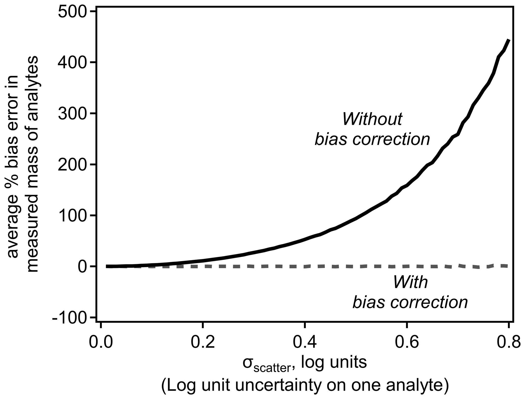
Figure 2Average of bias (percentage) in mass of one or multiple analytes with and without bias correction.
Equations (4) and (8) suggest two important conclusions: (1) summing multiple analytes reduces the uncertainty in the summed concentration, and (2) analytes and sums of analytes calibrated using log-transformed relationships are inherently biased. To explore the combined effects of these two conclusions, we perform a Monte Carlo analysis that simulates the real-world application of log-transformed sensitivity models. N number of simulated analytes are generated with a randomly assigned “true sensitivity” defined by the relationship shown in Fig. 1 with a Gaussian distribution of error, σ. Each analyte is assigned a random “true sampled mass” spanning 6 orders of magnitude (i.e., 10−3 to 103 arbitrary mass units). A simulated signal produced by each analyte is calculated by multiplying its true sensitivity by its true sampled mass. The nominal log-linear model is used to estimate a fitted sensitivity for each analyte, which is used to convert the signal to the fitted mass of an analyte. The summed fitted mass of all N analytes is compared to the summed true sampled mass to calculate the error in the fitted mass; 100 000 such simulations of N analytes yield a probability distribution of expected error.

Figure 3Probability distribution of percent error in the summed mass of N analytes based on the Monte Carlo analysis described in the text. Distributions of 5, 50, and 500 analytes are shown (a) without bias correction and (b) with bias correction using Eq. (8).
The combined effects of the two statistical trends implied by Eqs. (4) and (8) are clear in Fig. 3. As the number of analytes, N, increases, the sum of the mass converges toward a tighter distribution of uncertainty (i.e., the sum becomes less uncertain). However, the mass to which the distribution converges is inherently biased. In other words, the sum of five analytes may span a wide range of potential error, but on average they will be biased high by ∼ 50 %. Increasing the number of analytes just improves the probability that the sum is ∼ 50 % too high. The sum of 500 analytes, each with an uncertainty of a factor of 2.5 has high precision but inherently biased accuracy.
This approach assumes that true sensitivities are not perfectly represented by the nominal relationship (i.e., scatter is “real”); this is in contrast to the case in which each analyte is actually truly described by the fit and deviations are due to measurement uncertainties (i.e., scatter is measurement error). If the latter is discovered in subsequent literature to be the case, no bias would truly exist and the work in this paper would be extraneous. However, we believe the more likely case is that the scatter is a real consequence of the calibration approach for two reasons. Firstly, it is unlikely that an empirically derived relationship captures with perfect fidelity the sensitivity of an analyte. Secondly, because an iodide CIMS classifies analytes by elemental formula with no regard to molecular structure, the dV50 of each analyte (i.e., ion) is typically some combination of multiple compounds (Bi et al., 2021). It therefore inherently represents some composite of a distribution of analytes and is unlikely to equally represent all analytes in the mixture. Nevertheless, scatter measured by a real instrument provides some insight into true scatter; imperfect measurements of many compounds scattered around the nominal relationship would yield the nominal relationship with some uncertainty that represents the true variability (at least to some greater or lesser degree). For the purposes of real-world instruments, then, we suggest that it is reasonable to use observed uncertainty in model parameters as an estimate of their true variability and will do so throughout this work. However, we note that the sensitivity of some compounds predicted by the log-linear relationship between sensitivity and dV50 may have high uncertainty, likely due to the empirical nature of the relationship (Bi et al., 2021).

Figure 4Nominal (black line) log-linear relationship between sensitivity and dV50 following a typical iodide-CIMS calibration form, with labels on the four sources of uncertainty described in the text. Each circle represents one simulated ion generated from the log-linear relationship determined by Isaacman-Vanwertz et al. (2018) within a distribution of uncertainty defined by the values listed in the figure. The dashed line illustrates one possible relationship representing 1 standard deviation away from each nominal value. Note that the use of ΔdV50 in Eq. (9) has changed the sign of the slope compared to when it is plotted against dV50.
4.1 Sources of uncertainty
So far, this work has treated a fairly simple case: normally distributed error in log-transformed data. However, in the case of an iodide-CIMS calibration using voltage scans, this may not accurately represent the form of uncertainty. The true relationship between log(sensitivity) and dV50 has several parameters, each of which could be uncertain or may represent a central tendency of an inherently imperfect relationship. Figure 4 shows the nominal relationship between sensitivity and dV50 of a form that is typically considered for an iodide CIMS using voltage scans, as well as an illustrative potential spread of true sensitivities around this relationship. At some dV50, max, the instrument reaches maximum sensitivity, Smax, and it might be reasonable to expect that analytes closer to this value adhere more closely to the general relationship than compounds that diverge significantly from maximum sensitivity. In this case, variability in sensitivity may itself be partly (but perhaps only partly) a function of dV50 (i.e., heteroscedastic). Note that while compounds near maximum sensitivity are generally well predicted, the nominal relationship in Fig. 4 assumes that sensitivities of low-sensitivity analytes may diverge by roughly an order of magnitude from the general trend.
The relationship shown in Fig. 4 is defined by four critical parameters that may have some uncertainty or may deviate from the nominal relationship. The distribution of sensitivities can be described by some distribution in each of the four parameters, in the units and forms they have been previously considered (Isaacman-Vanwertz et al., 2018).
-
σscatter is the scatter in true sensitivity around the nominal relationship (i.e., the extent to which the average relationship inherently describes the data). Units are log units of sensitivity.
-
σslope is the variability in the slope of the relationship between log(sensitivity) and dV50. Units are log units of sensitivity per volt.
-
is the variability in the inflection point, the dV50 voltage at which sensitivity reaches its maximum. The unit is volts.
-
is the extent to which the nominal maximum sensitivity describes the sensitivity of compounds that are expected to be maximally sensitive. The unit is percent.
Each deviation from the nominal relationship will lead to inherent bias as in the simple log-transformed example discussed above. The exception to this issue is the fourth source of variability, variability in maximum sensitivity. Because this parameter is typically known reasonably well, uncertainty is low and best considered as a percentage. Uncertainty in this parameter is therefore not in log terms and does not introduce bias (i.e., 10 % lower and 10 % higher are equally different from the nominal maximum sensitivity).
4.2 Bias correction
To correct for the three potential sources of bias, we introduce Eq. (9) to calculate the expected sensitivity, S, of an analyte of a given dV50.
A critical term in this calculation is the extent to which the dV50 of an analyte is below the nominal inflection point dV50,max, which is defined as going to 0 in the region of maximum sensitivity, ΔdV50= max(dV50,max − dV50, 0). The use of ΔdV50 has changed the sign of the slope compared to when it is plotted against dV50 (top x axis in Fig. 4). The slope is defined as change in log(sensitivity) per unit ΔdV50 and is therefore necessarily a negative value (i.e., sensitivity decreases with ΔdV50). The first two terms in this equation (i.e., constitute the nominal relationship, while the last three terms introduce corrections for bias due to σscatter, σslope, and , respectively. We note that the first two terms are identical in form to the sensitivity equation used in previous work (Isaacman-Vanwertz et al., 2018), except Eq. (9) excludes an additional correction term (“S0”) that is outside the scope of the present work but is typically included to account for partial declustering at ΔdV50=0.
Unlike in the simple case of σscatter, note that bias correction factors for σslope and are not independent of parameters in the nominal relationship. Bias caused by σslope increases with the range of dV50 across which the relationship is applied. Bias caused by increases with the slope, which makes sense when considered at its extreme – if there were no decrease in sensitivity with dV50, then the inflection point is irrelevant. Given these dependencies, the scope of bias and the efficacy of the bias correction term must be explored using some approximation of typical CIMS conditions. For this work we use the calibration parameters used by Isaacman-Vanwertz et al. (2018): d V, slope = −0.9 log units sensitivity per volt, up to a maximum ΔdV50=2.3 (a minimum effective sensitivity was applied by Isaacman-Vanwertz et al. (2018), which is irrelevant to this work). Using these bounding conditions, the bias introduced by the model parameters is shown in Fig. 5, in which the other sources of variability are held at 0 to isolate the effect of each parameter. As in Fig. 2, bias quickly increases with σ for all parameters except (as expected). The correction factors introduced in Eq. (9) almost fully remove all bias.
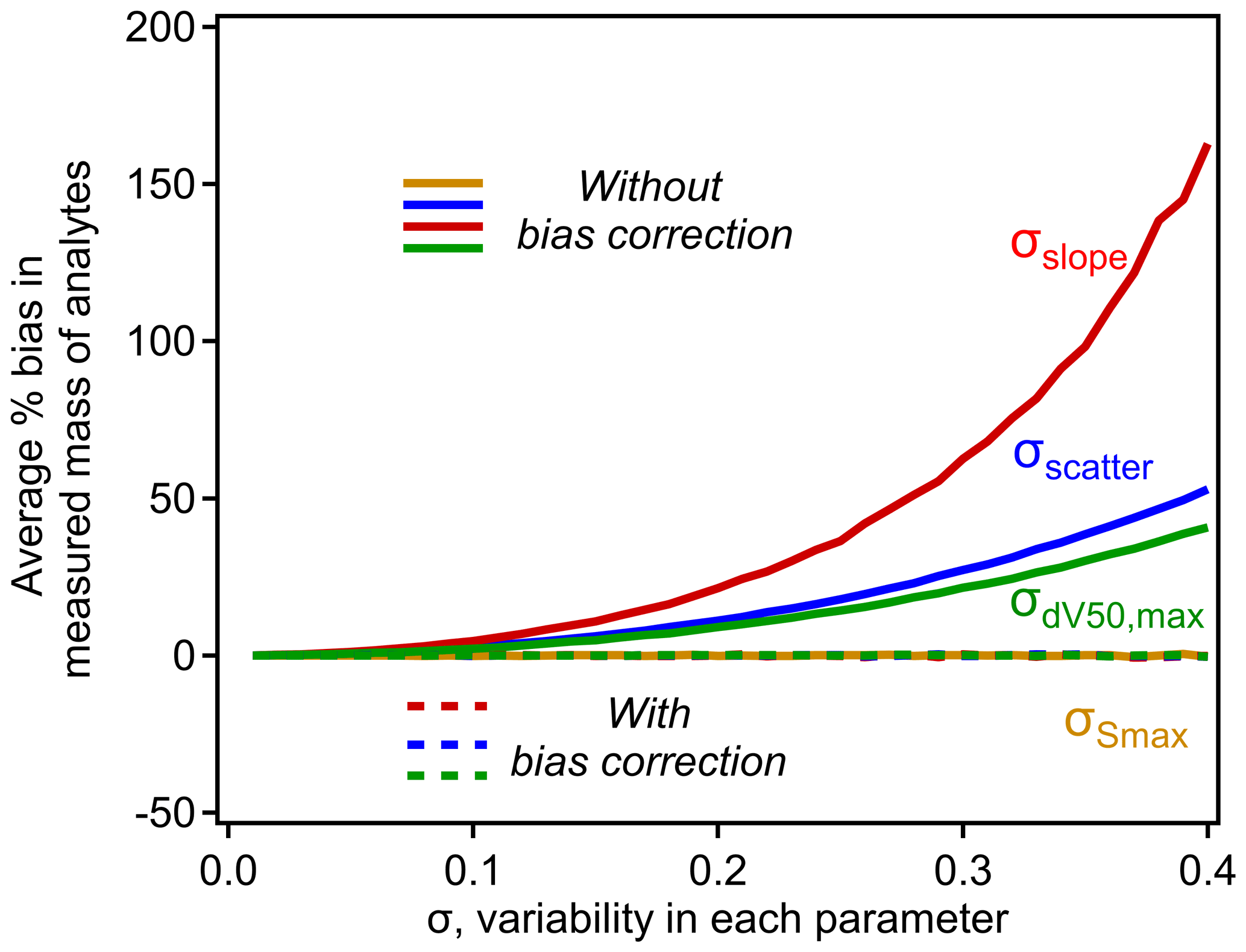
Figure 5The influence of σscatter, σslope, , and on the average percent bias in analytes calibrated using the typical iodide–CIMS relationship shown in Fig. 4. Each curve is calculated empirically using a simulation of N=106 analytes, with operating conditions of d V, slope = −0.9 log units sensitivity per volt, up to a maximum ΔdV50=2.3, following Isaacman-VanWertz et al. (2018). Uncertainty in each parameter not being investigated is held at 0.
To examine the combined effect of variability in all four parameters, we investigate the conditions described for a real-world iodide CIMS by Isaacman-Vanwertz et al. (2018). Uncertainty was estimated based on reported values in that work: σscatter= 0.2 log units, σslope= 0.125 log units per volt, volts, and % (calculated as the approximate standard deviation of their two reported possible values for Smax). No value for σscatter was actually reported as no measurements were available to constrain the inherent scatter in sensitivity, so 0.2 log units is assigned here as an estimate that produces approximately the same average uncertainty reported in that work for individual ions (a factor of ∼ 2.5).

Figure 6Errors in summed mass of ions with and without bias corrections in the case study of the CIMS conditions described by Isaacman-VanWertz et al. (2018), represented by the listed uncertainties and number of analytes. Probability distributions of errors are shown for calibration without including any bias correction (red), including the parameter-explicit bias correction described by Eq. (9) (blue) and including the simplified bias correction described by Eqs. (10) and (11) (green).
The example shown in Fig. 6 provides a case study to examine the importance and the limitations of bias correction. Without introducing the correction parameters, the sum of 225 analytes (ions measured by iodide CIMS) is expected to yield a mass roughly 30 % too high, with a range of possible measurements spanning from negative error to nearly a factor of 2. As described in Sect. 2.2, this 30 % bias in the sum is caused by an average 30 % in each individual analyte, so the bias exists for one analyte as well as for the sum of analytes. Introducing the correction parameters in Eq. (9) removes this bias and tightens the distribution, but the range of possible sums is still substantial. In the work upon which this case study is based, Isaacman-VanWertz et al. (2018) used a similar Monte Carlo approach to calibrate all ions, explicitly considering a distribution of uncertainty in calibration parameters, so likely avoided introducing bias. Notably, they estimated that a factor of 3 uncertainty in any given analyte led to an uncertainty of ∼ 60 % in the sum of the 225 ions measured, comparable to the width of the distribution shown in Fig. 6. The approach described here alleviates the need to perform a full Monte Carlo approach in future work seeking to calibrate large numbers of ions, instead using Eq. (9) to remove the bias in average sensitivities.
To remove bias in CIMS calibration, the correction terms in Eq. (9) should be included in the calculation of an analyte's sensitivity. However, in many real-world cases, the number of calibrants to establish the log-linear relationship is limited (e.g., fewer than 10 in Lopez-Hilfiker et al., 2016; Mattila et al., 2020), so it may not be feasible to separately treat uncertainty in all four parameters. A simplification of the detailed, parameter-explicit approach here could instead treat all forms of uncertainty as some average residual between the nominal and true sensitivities with an effective scatter, . Such an approach would apply only the first correction term using this average scatter, ignoring the terms dependent on dV50 and slope and implicitly assumes that uncertainty is homoscedastic. This simplified approach, shown below in Eq. (10), is mathematically equivalent to the basic log-transformed case of Eq. (8) and roughly works for low to moderate but loses skill as the slope and the range in dV50 increase.
Application of Eq. (10) represents a more feasible approach to the implementation of bias correction under many real-world scenarios than the full, parameter-explicit form of Eq. (9) but requires a careful consideration of the best approach to estimate . In the specific case that σscatter is the only source of uncertainty (i.e., ), must equal σscatter and error is homoscedastic. Because σscatter is by definition a description of the error in the model relationship, it can be estimated as the standard deviation of the residual of the log-linear fit (σresidual), and this value must represent a reasonable estimate of . However, a non-negligible caveat to this approach is that quantitatively impacts the residual of the log-linear fit but does not introduce bias and thus should not influence the bias correction term. Consequently, the effect of needs to be removed from the residual before using it as an estimate of . Fortunately, uncertainty in Smax is often reasonably well constrained based on experimental parameters (e.g., uncertainty in the calibration of a maximum sensitivity analyte), so can be estimated as
where is the log-equivalent uncertainty in Smax, which is typically considered in linear terms. For example in the case of % (i.e., a factor of 0.9), the log-equivalent uncertainty is log(0.9) × (−1) = 0.045. This linear-to-log conversion is only meaningful for relatively low uncertainty (⪅ 50 %), for which can be estimated as
For uncertainty in beyond 50 %, the conversion is provided as Eq. (S1), but uncertainty is probably sufficiently high that it should be considered in log terms in any case. In some cases, may not be available, so in the Supplement, we examine alternative statistical parameters as but find that Eq. (11) is most effective in eliminating the bias.
Table 1Step-by-step guidance to apply the simplified bias correction method.

∗ Equation (S1) should be used to calculate when %.
As shown in Fig. 6 (green line), the average bias in the calibrated mass of analytes can be fully eliminated using the simplified bias corrections. However, a significant shortcoming of this simplified approach is its implicit assumption of homoscedastic error. Some single average correction will necessarily underestimate the bias in some analytes and overestimate the bias in others. Because uncertainty is expected to increase with decreasing sensitivity, this simplified correction will lead to a systematic bias toward overcorrecting high-sensitivity analytes and undercorrecting low-sensitivity analytes. This issue is demonstrated in Fig. 7, in which the simplified bias correction (green line) represents some average representation of the true bias correction (blue). The effect of this issue is strongly dependent on the relative importance of each source of error. Limitations of the simplified approach are more severe in cases where heteroscedastic errors (e.g., σslope) are significant (Fig. S5). Not enough data are yet available in the literature to determine the relative importance of uncertainties in each parameter, so the potential downsides of the simplified approach are not yet well constrained. Therefore, parameter-explicit bias correction should be implemented in cases where all four parameters can be reasonably estimated, but a simplified approach remains reasonable.
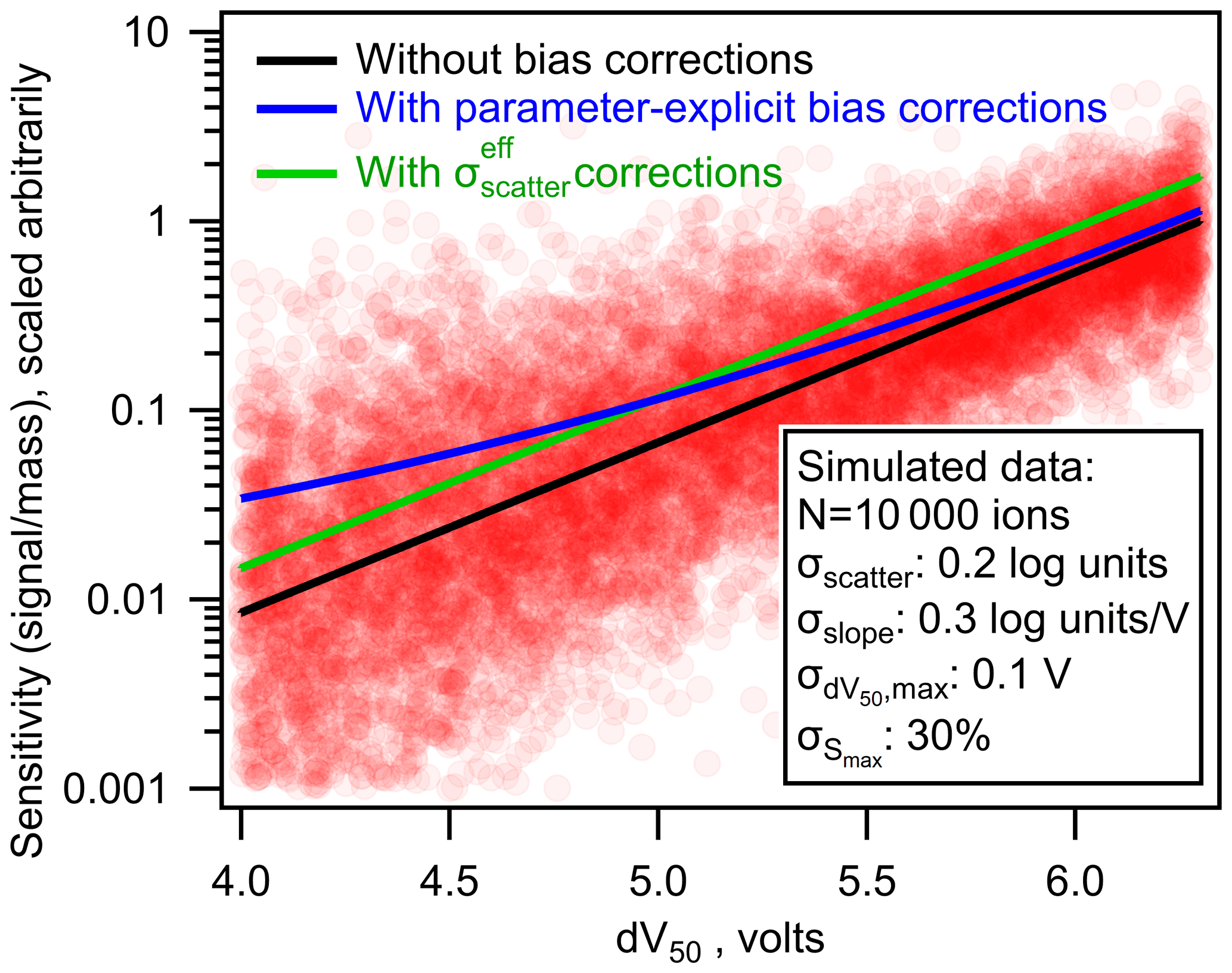
Figure 7The nominal (black line), parameter-explicit bias-corrected (blue line), and bias-corrected (green line) log-linear relationship between sensitivity and dV50. Each pink circle represents one simulated ion generated from the log-linear relationship determined by Isaacman-Vanwertz et al. (2018) with uncertainties replaced with those listed in the figure.
An additional value of is that it can be considered an indicator of magnitude of the potential bias in retrospective analyses of past datasets. In two previous studies implementing the voltage scan calibration, we found that the calculated can be as low as 0.012 (Mattila et al., 2020), or as high as 0.29 (Lopez-Hilfiker et al., 2016; Iyer et al., 2016). Based on the log-linear fit and the calculated in the two previous studies, the average bias in the summed mass of 100 simulated ions would be approximately 2 % and 28 % in Mattila et al. (2020) and Lopez-Hilfiker et al. (2016), respectively, if sensitivities were determined by voltage scanning. However, these two extremes represent voltage scanning of two different instrument voltage regions and are calculated using a limited number of calibrants. The potential range of the therefore remains unclear, and future work is needed to examine this approach in real-world applications, and the real potential for bias in voltage scanning approaches. Furthermore, the number of calibrants in a voltage scan calibration is often limited due to the lack of commercially available standards covering the entire sensitivity range, so σresidual (and thus may not adequately capture the true scatter of residuals.
Uncertainty of instrumental measurements is frequently reported in the literature, which is typically a measure of the combined instrument precision and accuracy. In contrast, bias represents a systematic error in the accuracy and is distinct from these reported uncertainties. It is theoretically worth comparing the relative magnitude of the two types of errors, as a small bias would likely be negligible in the case of large uncertainty. However, this is difficult as bias may vary significantly depending on the uncertainties of the log-linear fit, with examples shown in Fig. S5 ranging from 8 % to 300 % bias in summed mass of analytes. Recent work by Bi et al. (2021) found uncertainties of a factor of 3–10 for individual ions and ∼ 30 % for the sum of many ions using the voltage scanning method. This summed uncertainty is comparable in scale to the bias determined for the data from Isaacman-VanWertz et al. (2018), indicating bias is likely non-negligible. For individual ions, the importance of bias correction depends strongly on the dV50 of the compound and the scale of the bias correction, though a parameter-explicit bias correction always increases accuracy.
In this work, we examine uncertainty in the case where instrument sensitivity is itself a function of some parameter, with a focus on uncertainty in the summation of multiple analytes. We show that when sensitivity is a linear function of a parameter, the sum of multiple analytes necessarily has lower relative uncertainty than any given analyte. However, when an iodide CIMS is calibrated by the voltage scanning method utilizing the linear relationship between log transformation of sensitivity and a parameter, an inherent bias is introduced into the sensitivity of analytes. While summing multiple analytes increases the precision of the sum, the bias can only be eliminated by specifically introducing correction terms to the relationship. Although the discussions of this work mainly focus on iodide CIMS, we believe that this correction can be applied to other CIMSs or more broadly other atmospheric measurement instruments using log-linear calibration relationships.
The correction terms introduced in this work for both the general case of log-transformed relationships and the special case of an iodide CIMS (i.e., Eq. 9), fully remove this bias. We propose that these correction terms should be introduced into any such calibration schemes in future work in order to minimize bias and reduce uncertainty in the literature. Given that real-world calibration scenarios are complex and consequently not all parameters have known uncertainties, we suggest that, at least, a term to correct for the average observed scatter around the nominal relationship, i.e., Eq. (10), should be incorporated in calibrations to remove a major portion of the bias. For the convenience of method users, we summarize correction procedures as a step-by-step guidance to apply the simplified bias correction method in Table 1.
However, we do recommend that this simplified approach be used cautiously to avoid overcorrections of sensitivity for more sensitive analytes and undercorrections for less sensitive ones. While data are limited on the uncertainty in each calibration parameter and the relative merits of simplified vs. parameter-explicit correction, bias-corrected results are expected to be more accurate than uncorrected values, and some form of bias correction should be introduced into instrument calibrations relying on log-transformed calibrations.
All raw and processed data collected as part of this project are available upon request.
The supplement related to this article is available online at: https://doi.org/10.5194/amt-14-6551-2021-supplement.
GIVW developed the thought experiment. CB led the consequent data simulation and analysis under the guidance of GIVW. JEK and MRC contributed to the development of the theory of the described approach. CB and GIVW prepared the manuscript with contributions from all other authors.
Jordan E. Krechmer and Manjula R. Canagaratna are employed by Aerodyne Research, Inc., which commercializes CIMS instruments for geoscience research.
Publisher’s note: Copernicus Publications remains neutral with regard to jurisdictional claims in published maps and institutional affiliations.
We would like to thank the Alfred P. Sloan Foundation Chemistry of the Indoor Environment Program for supporting this work.
This research has been supported by the Alfred P. Sloan Foundation (grant no. P-2018-11129).
This paper was edited by Glenn Wolfe and reviewed by two anonymous referees.
Bertram, T. H., Kimmel, J. R., Crisp, T. A., Ryder, O. S., Yatavelli, R. L. N., Thornton, J. A., Cubison, M. J., Gonin, M., and Worsnop, D. R.: A field-deployable, chemical ionization time-of-flight mass spectrometer, Atmos. Meas. Tech., 4, 1471–1479, https://doi.org/10.5194/amt-4-1471-2011, 2011.
Bi, C., Krechmer, J. E., Frazier, G. O., Xu, W., Lambe, A. T., Claflin, M. S., Lerner, B. M., Jayne, J. T., Worsnop, D. R., Canagaratna, M. R., and Isaacman-VanWertz, G.: Coupling a gas chromatograph simultaneously to a flame ionization detector and chemical ionization mass spectrometer for isomer-resolved measurements of particle-phase organic compounds, Atmos. Meas. Tech., 14, 3895–3907, https://doi.org/10.5194/amt-14-3895-2021, 2021.
Brophy, P.: Development, characterization, and deployment of a high-resolution time-of-flight chemical ionization mass spectrometer (hr-tof-cims) for the detection of carboxylic acids and trace-gas species in the troposphere, Colorado State University, 1–215, 2016.
Brophy, P. and Farmer, D. K.: Clustering, methodology, and mechanistic insights into acetate chemical ionization using high-resolution time-of-flight mass spectrometry, Atmos. Meas. Tech., 9, 3969–3986, https://doi.org/10.5194/amt-9-3969-2016, 2016.
Crounse, J. D., McKinney, K. A., Kwan, A. J., and Wennberg, P. O.: Measurement of gas-phase hydroperoxides by chemical ionization mass spectrometry, Anal. Chem., 78, 6726–6732, https://doi.org/10.1021/ac0604235, 2006.
Hurley, J. F., Kreisberg, N. M., Stump, B., Bi, C., Kumar, P., Hering, S. V., Keady, P., and Isaacman-VanWertz, G.: A new approach for measuring the carbon and oxygen content of atmospherically relevant compounds and mixtures, Atmos. Meas. Tech., 13, 4911–4925, https://doi.org/10.5194/amt-13-4911-2020, 2020.
Isaacman-VanWertz, G., Massoli, P., O'Brien, R. E., Nowak, J. B., Canagaratna, M. R., Jayne, J. T., Worsnop, D. R., Su, L., Knopf, D. A., Misztal, P. K., Arata, C., Goldstein, A. H., and Kroll, J. H.: Using advanced mass spectrometry techniques to fully characterize atmospheric organic carbon: Current capabilities and remaining gaps, Faraday Discuss., 200, 579–598, https://doi.org/10.1039/c7fd00021a, 2017.
Isaacman-Vanwertz, G., Massoli, P., O'Brien, R., Lim, C., Franklin, J. P., Moss, J. A., Hunter, J. F., Nowak, J. B., Canagaratna, M. R., Misztal, P. K., Arata, C., Roscioli, J. R., Herndon, S. T., Onasch, T. B., Lambe, A. T., Jayne, J. T., Su, L., Knopf, D. A., Goldstein, A. H., Worsnop, D. R., and Kroll, J. H.: Chemical evolution of atmospheric organic carbon over multiple generations of oxidation, Nat. Chem., 10, 462–468, https://doi.org/10.1038/s41557-018-0002-2, 2018.
Iyer, S., Lopez-Hilfiker, F., Lee, B. H., Thornton, J. A., and Kurtén, T.: Modeling the Detection of Organic and Inorganic Compounds Using Iodide-Based Chemical Ionization, J. Phys. Chem. A, 120, 576–587, https://doi.org/10.1021/acs.jpca.5b09837, 2016.
Jokinen, T., Sipilä, M., Junninen, H., Ehn, M., Lönn, G., Hakala, J., Petäjä, T., Mauldin, R. L., Kulmala, M., and Worsnop, D. R.: Atmospheric sulphuric acid and neutral cluster measurements using CI-APi-TOF, Atmos. Chem. Phys., 12, 4117–4125, https://doi.org/10.5194/acp-12-4117-2012, 2012.
Krechmer, J. E., Coggon, M. M., Massoli, P., Nguyen, T. B., Crounse, J. D., Hu, W., Day, D. A., Tyndall, G. S., Henze, D. K., Rivera-Rios, J. C., Nowak, J. B., Kimmel, J. R., Mauldin, R. L., Stark, H., Jayne, J. T., Sipilä, M., Junninen, H., St. Clair, J. M., Zhang, X., Feiner, P. A., Zhang, L., Miller, D. O., Brune, W. H., Keutsch, F. N., Wennberg, P. O., Seinfeld, J. H., Worsnop, D. R., Jimenez, J. L., and Canagaratna, M. R.: Formation of Low Volatility Organic Compounds and Secondary Organic Aerosol from Isoprene Hydroxyhydroperoxide Low-NO Oxidation, Environ. Sci. Technol., 49, 10330–10339, https://doi.org/10.1021/acs.est.5b02031, 2015.
Lee, B. H., Lopez-Hilfiker, F. D., Mohr, C., Kurtén, T., Worsnop, D. R., and Thornton, J. A.: An iodide-adduct high-resolution time-of-flight chemical-ionization mass spectrometer: Application to atmospheric inorganic and organic compounds, Environ. Sci. Technol., 48, 6309–6317, https://doi.org/10.1021/es500362a, 2014.
Lindinger, W., Hansel, A., and Jordan, A.: On-line monitoring of volatile organic compounds at pptv levels by means of Proton-Transfer-Reaction Mass Spectrometry (PTR-MS) Medical applications, food control and environmental research, Int. J. Mass Spectrom., 173, 191–241, 1998.
Lopez-Hilfiker, F. D., Iyer, S., Mohr, C., Lee, B. H., D'Ambro, E. L., Kurtén, T., and Thornton, J. A.: Constraining the sensitivity of iodide adduct chemical ionization mass spectrometry to multifunctional organic molecules using the collision limit and thermodynamic stability of iodide ion adducts, Atmos. Meas. Tech., 9, 1505–1512, https://doi.org/10.5194/amt-9-1505-2016, 2016.
Mattila, J. M., Lakey, P. S. J., Shiraiwa, M., Wang, C., Abbatt, J. P. D., Arata, C., Goldstein, A. H., Ampollini, L., Katz, E. F., Decarlo, P. F., Zhou, S., Kahan, T. F., Cardoso-Saldaña, F. J., Ruiz, L. H., Abeleira, A., Boedicker, E. K., Vance, M. E., and Farmer, D. K.: Multiphase Chemistry Controls Inorganic Chlorinated and Nitrogenated Compounds in Indoor Air during Bleach Cleaning, Environ. Sci. Technol., 54, 1730–1739, https://doi.org/10.1021/acs.est.9b05767, 2020.
Miller, D. M.: Reducing Transformation Bias in Curve Fitting, Am. Statist., 38, 124–126, 1984.
Riva, M., Rantala, P., Krechmer, E. J., Peräkylä, O., Zhang, Y., Heikkinen, L., Garmash, O., Yan, C., Kulmala, M., Worsnop, D., and Ehn, M.: Evaluating the performance of five different chemical ionization techniques for detecting gaseous oxygenated organic species, Atmos. Meas. Tech., 12, 2403–2421, https://doi.org/10.5194/amt-12-2403-2019, 2019.
Sekimoto, K., Li, S.-M., Yuan, B., Koss, A., Coggon, M., Warneke, C., and de Gouw, J.: Calculation of the sensitivity of proton-transfer-reaction mass spectrometry (PTR-MS) for organic trace gases using molecular properties, Int. J. Mass Spectrom., 421, 71–94, https://doi.org/10.1016/j.ijms.2017.04.006, 2017.
Slusher, D. L.: A thermal dissociation–chemical ionization mass spectrometry (TD-CIMS) technique for the simultaneous measurement of peroxyacyl nitrates and dinitrogen pentoxide, J. Geophys. Res., 109, 1–19, https://doi.org/10.1029/2004jd004670, 2004.
St Clair, J. M., McCabe, D. C., Crounse, J. D., Steiner, U., and Wennberg, P. O.: Chemical ionization tandem mass spectrometer for the in situ measurement of methyl hydrogen peroxide, Rev. Sci. Instrum., 81, 094102, https://doi.org/10.1063/1.3480552, 2010.
Yuan, B., Koss, A., Warneke, C., Gilman, J. B., Lerner, B. M., Stark, H., and De Gouw, J. A.: A high-resolution time-of-flight chemical ionization mass spectrometer utilizing hydronium ions (H3O+ ToF-CIMS) for measurements of volatile organic compounds in the atmosphere, Atmos. Meas. Tech., 9, 2735–2752, https://doi.org/10.5194/amt-9-2735-2016, 2016.
Zaytsev, A., Breitenlechner, M., Koss, A. R., Lim, C. Y., Rowe, J. C., Kroll, J. H., and Keutsch, F. N.: Using collision-induced dissociation to constrain sensitivity of ammonia chemical ionization mass spectrometry (NH CIMS) to oxygenated volatile organic compounds, Atmos. Meas. Tech., 12, 1861–1870, https://doi.org/10.5194/amt-12-1861-2019, 2019.
- Abstract
- Introduction
- Prior work on uncertainty analysis
- Method for quantifying error in sums of analytes
- Expanding to CIMS-specific parameters
- Corrections in real-world applications
- Conclusions
- Data availability
- Author contributions
- Competing interests
- Disclaimer
- Acknowledgements
- Financial support
- Review statement
- References
- Supplement