Gravity wave instability structures and turbulence from more than 1.5 years of OH* airglow imager observations in Slovenia

We analysed 286 nights of data from the OH* airglow imager FAIM 3 (Fast Airglow IMager) acquired at Otlica Observatory (45.93^∘ N, 13.91^∘ E), Slovenia, between 26 October 2017 and 6 June 2019. Measurements have been performed with a spatial resolution of 24 m per pixel and a temporal resolution of 2.8 s.

A two-dimensional fast Fourier transform is applied to the image data to derive horizontal wavelengths between 48 m and 4.5 km in the upper mesosphere/lower thermosphere (UMLT) region. In contrast to the statistics of larger-scale gravity waves (horizontal wavelength up to ca. 50 km; Hannawald et al., 2019), we find a more isotropic distribution of directions of propagation, pointing to the presence of wave structures created above the stratospheric wind fields. A weak seasonal tendency of a majority of waves propagating eastward during winter may be due to instability features from breaking secondary gravity waves that were created in the stratosphere. We also observe an increased southward propagation during summer, which we interpret as an enhanced contribution of secondary gravity waves created as a consequence of primary wave filtering by the meridional mesospheric circulation.

We present multiple observations of turbulence episodes captured by our high-resolution airglow imager and estimated the energy dissipation rate in the UMLT from image sequences in 25 cases. Values range around 0.08 and 9.03 W kg⁻¹ and are on average higher than those in recent literature. The values found here would lead to an approximated localized maximum heating of 0.03–3.02 K per turbulence event. These are in the same range as the daily chemical heating rates for the entire atmosphere reported by Marsh (2011), which apparently stresses the importance of dynamical energy conversion in the UMLT.

1 Introduction

Fully understanding the contribution of gravity waves to atmospheric dynamics is still a major issue when establishing climate models. Due to the various sources and mechanisms of interactions, the effects of gravity waves have to be represented in these models using advanced parameterizations (Lindzen, 1981; Holton, 1983; de la Cámara et al., 2016) to cover as many aspects as is possible given the restricted model resolution. Gravity waves exist on a large span of timescales ranging from several hours down to the Brunt–Väisälä (BV) period, which corresponds to ca. 4–5 min in the upper mesosphere/lower thermosphere (UMLT) region (Wüst et al., 2017b) and represents the smallest possible period of gravity waves. They show diverse behaviour depending strongly on wave properties like their periodicity (Fritts and Alexander, 2003; Beldon and Mitchell, 2009; Hoffmann et al., 2010; Wüst et al., 2016; Sedlak et al., 2020), which makes it even harder to fully account for them by means of parameterization. Furthermore, gravity wave generation is not restricted to the troposphere but can also take place at higher altitudes, such as secondary wave excitation due to breaking gravity waves (see, for example, Holton and Alexander, 1999; Satomura and Sato, 1999; Vadas and Fritts, 2001; Becker and Vadas, 2018).

As Fritts and Alexander (2003) state, it is necessary to metrologically capture all parts of the gravity wave spectrum. This includes especially dynamics on short scales where gravity wave breaking is induced by the development of instabilities. One of the most prominent features in this context is the formation of Kelvin–Helmholtz instability (KHI), which occurs as a consequence of a dynamically unstable atmosphere due to wind shear (Browning, 1971). Gravity wave instability can also be of convective nature when growing wave amplitudes lead to a superadiabatic lapse rate (Fritts and Alexander, 2003). In general, atmospheric instabilities like KHIs often manifest as so-called ripples – periodic structures with small spatial dimensions and short lifetimes (Peterson, 1979; Adams et al., 1988; Taylor and Hapgood, 1990; Li et al., 2017).

Gravity wave breaking and the conversion of the transported energy into heat takes place in the course of turbulence. Once a wave breaks and motion shifts from laminar to turbulent flow, energy is cascaded to smaller and smaller structures until viscosity becomes dominant over inertia, and energy is dissipated into the atmosphere by viscous damping (see, for example, Lübken et al., 1987).

The process of turbulence manifests as formation of vortices, so-called eddies. They cause turbulent mixing of the medium, resulting in the dissipation of turbulent energy at an energy dissipation rate ϵ. According to the theory of stratified turbulence, ϵ depends on the characteristic length scale L and velocity scale U of the turbulent features. The energy dissipation rate is then given by

$$\begin{array}{}\text{(1)}& \mathit{ϵ}=C_{\mathit{ϵ}}{\displaystyle \frac{U^{\mathrm{3}}}{L}}\end{array}$$

(see, for example, Chau et al., 2020, who apply this equation to radar observations of KHIs). C_ϵ is a constant which is found to be equal to 1 (Gargett, 1999).

Gravity wave dissipation predominantly occurs in the upper mesosphere/lower thermosphere (UMLT) region (Gardner et al., 2002). Hocking (1985) states that the turbulent regime at this altitude manifests on scales shorter than 1 km, which sets high requirements for measurement techniques at these heights. This is why turbulence investigations in the UMLT are challenging, and there are only few values of ϵ available at UMLT heights. Lübken (1997) use rocket measurements to retrieve ϵ in the height range 65–120 km. Baumgarten and Fritts (2014) use imaging techniques of mesospheric noctilucent clouds to investigate the formation of KHIs and the onset of turbulence.

At the same height, remote sensing measurements of the OH* airglow are an established access to UMLT dynamics. The OH* airglow is a layer at an average altitude of ca. 86–87 km with a full width at half maximum (FWHM) of ca. 8 km (Baker and Stair, 1988; Liu and Shepherd, 2006; Wüst et al., 2017b). Remote sensing techniques include spectroscopic measurements of strong emission lines and the analysis of temperature time series derived from these (Hines and Tarasick, 1987; Mulligan et al., 1995; Bittner et al., 2000; Reisin and Scheer, 2001; Espy and Stegman, 2002; Espy et al., 2003; French and Burns, 2004; Offermann et al., 2009; Schmidt et al., 2013, 2018; Wachter et al., 2015; Silber et al., 2016; Wüst et al., 2016, 2017a, 2018) but also two-dimensional imaging in the short-wave infrared (SWIR) range (see, for example, Peterson and Kieffaber, 1973; Hecht et al., 1997; Taylor, 1997; Moreels et al., 2008; Li et al., 2011; Pautet et al., 2014; Hannawald et al., 2016, 2019; Sedlak et al., 2016; Wüst et al., 2019, and many more).

The technology of OH* imaging has undergone a rapid technical progress over the last few decades. Improvements in sensor technology and optics have provided the possibility to observe the signatures of gravity waves that manifest as periodic brightness variations in infrared images of the OH* airglow layer. The observations range from all-sky imaging of large-scale gravity waves (e.g., Taylor, 1997; Smith et al., 2009) to high-resolution images of smaller gravity waves (Nakamura et al., 1999) and their breaking processes (Hecht et al., 2014; Hannawald et al., 2016). Hannawald et al. (2016) use an airglow imager called FAIM (Fast Airglow IMager) that is well suited for the observation of small-scale gravity waves with a high temporal resolution of 0.5 s. Based on 3 years of continuous night-time observations at two different Alpine locations, Hannawald et al. (2019) show statistics of gravity wave propagation for waves with horizontal wavelengths smaller than 50 km based on data of the same kind of instrument.

In 2016 we put into operation another FAIM instrument (FAIM 3) which still has a high temporal resolution of 2.8 s but also a high spatial resolution of up to 17 m per pixel (measurements in zenith direction utilizing a 100 mm SWIR objective lens). We were not only able to observe wave patterns on extraordinary small scales (smallest horizontal wavelength 550 m) but also the formation of a vortex which we interpret as the turbulent breakdown of a wave front (Sedlak et al., 2016).

From October 2017 to June 2019 the instrument observed the area around the Gulf of Trieste from Otlica Observatory, Slovenia (45.93^∘ N​​​​​​​, 13.91^∘ E), which is a partner observatory within the context of the Virtual Alpine Observatory (VAO; https://www.vao.bayern.de, last access: 16 October 2021​​​​​​​). This larger database includes further observations of small-scale wave features and turbulence which are investigated here.

The focus of this paper is on analysing small-scale dynamics in the UMLT region in FAIM 3 images with regard to two aspects:

1. We perform a statistical analysis of wave parameters on scales below 4.5 km using a two-dimensional fast Fourier transform (2D-FFT). Using the same measurement technique and analysis, we are able to directly connect to the short-scale end of the investigations performed by Hannawald et al. (2019).

2. We estimate the dissipated energy by analysing multiple episodes of turbulence (such as the one exemplarily presented in Sedlak et al., 2016).

2 Instrumentation

FAIM 3 is an OH* airglow imager that has been put into operation in February 2016 at the German Aerospace Center (DLR) in Oberpfaffenhofen, Germany. It consists of the SWIR camera CHEETAH CL manufactured by Xenics NV, which has a thermodynamically cooled 640 × 512 pixels InGaAs sensor array (pixel size 20 µm × 20 µm, operating temperature 233 K). The camera is sensitive to electro-magnetic radiation in the wavelength range from 0.9 to 1.7 µm (for further technical details see Sedlak et al., 2016).

From 26 October 2017 to 6 June 2019 automatic measurements with focus on the OH* airglow emissions have been performed at Otlica Observatory (OTL) (45.93^∘ N​​​​​​​, 13.91^∘ E), Slovenia. FAIM 3 was aligned at a zenith angle of 35^∘ and an azimuthal direction of 240^∘ (facing approximately into WSW direction). Measurements are only possible during night-time because OH* emissions are not detectable in the presence of the much stronger solar radiation. A baffle was attached to prevent the images from being disturbed by reflections from the lab interior, e.g., by moon light. As in Sedlak et al. (2016) the camera was equipped with a 100 mm SWIR lens by Edmund Optics^® with aperture angles of 7.3 and 5.9^∘ in horizontal and vertical direction. Neglecting the curvature of the Earth, this configuration leads to a trapezium-shaped field of view (FOV) with a size of ca. 182 km² (13.1–14.1 km × 13.4 km) at the mean peak emission height of the OH* layer at ca. 87 km. The mean spatial resolution is therefore 24 m per pixel. Due to the above-mentioned measurement geometry the FOV is located above the Gulf of Trieste. The integration time of FAIM 3 is 2.8 s, which leads, depending on the season, to the acquisition of ca. 10 000 to 18 000 images per night.

3 Database

All in all, image data were acquired by FAIM 3 at OTL in 477 nights. Since OH* airglow observations are only possible under clear-sky conditions, cloudy episodes are filtered out by analysing keograms. This yields 410 clear-sky episodes (durations between 20 min and 13 h) that are distributed over 286 measurement nights. Thus, ca. 60 % of the acquired nights at OTL include suitable OH* observations.

Before being analysed, the images undergo the same preprocessing steps as in Hannawald et al. (2016, 2019) and Sedlak et al. (2016): a flat-field correction is performed, and the images are transferred to an equidistant grid, which corresponds to a trapezium-shaped FOV due to the inclination from zenith. For each episode, the average image is subtracted to ensure that all remnants of fixed patterns are removed (e.g., reflections of the objective lens in the laboratory window during bright nights). Due to the small FOV of FAIM 3, we renounce the application of a star removal algorithm to avoid an interpolation of too many pixels. In order to extract periodic signatures, a two-dimensional fast Fourier transform (2D-FFT) is applied to squared cut-outs of each image, so neither dimension is favoured by the analysis. These cut-outs were chosen to have a side length of 406 pixels (equals ca. 9.7 km) as this is the largest possible square fitting into the transformed images. The 2D-FFT is performed on the squared image cut-out as described by Hannawald et al. (2019). A fitted linear intensity gradient is subtracted from the input images, and a Hann window is applied during the 2D-FFT to reduce leakage effects. A local maximum filter is applied to automatically find peaks in the spectra and thus plane wave structures, which allows for identifying and analysing single wave events. Zero-padding on the images (to a size of 2160 × 2160 pixels) is used to improve this identification of peaks in the spectra. Hannawald et al. (2019) present a statistical analysis of gravity waves with horizontal wavelengths between 2 and 62 km (with focus on waves with horizontal wavelengths larger than 15 km). With FAIM 3 having a smaller FOV and a higher spatial resolution than the FAIM instrument used therein, we are now able to present statistics of gravity wave parameters that tie in almost seamlessly with the statistics of longer-scale waves of Hannawald et al. (2019): due to the spatial resolution and the FOV size, we cover the horizontal wavelength range from 48 m to 4.5 km. Wave structures with horizontal wavelengths of half the FOV size still showed a strong bias toward phases 0 or π. Extensive testing showed that this effect disappeared when lowering the upper wavelength limit to 4.5 km.

Observed wave structures have to meet several quality criteria in order to be considered a wave event. A wave structure has to be present for at least 20 s and has to be found in at least eight images. This is in contrast to Hannawald et al. (2019), who demand wave signatures to be present for at least 120 s and to appear in at least 100 images within this episode, stating that these restrictions specifically filter out many transient and small-scale wave features as they want to focus on larger persistent waves.

Furthermore, FAIM 3 wave events are considered if they have an amplitude of at least 25 % of the maximum observed wave amplitude. Wave structures with this amplitude can just be recognized in the image by eye. Demanding all the quality criteria mentioned above, a total number of 5697 wave events remains. Further restricting these criteria has not significantly altered the distributions of the wave parameters that are presented in the following. An exemplary event and the respective two-dimensional spectrum are shown in Fig. 1.

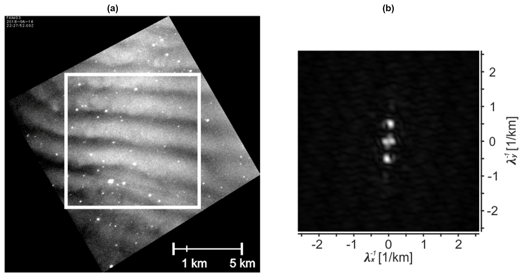
Figure 1 Event from 16 June 2018 22:27:52 UTC. The structure has a horizontal “wavelength” of ca. 1.9 km and extends over the entire image (a). The white square marks the area which is analysed with the 2D-FFT. The respective two-dimensional spectrum is shown in panel (b).

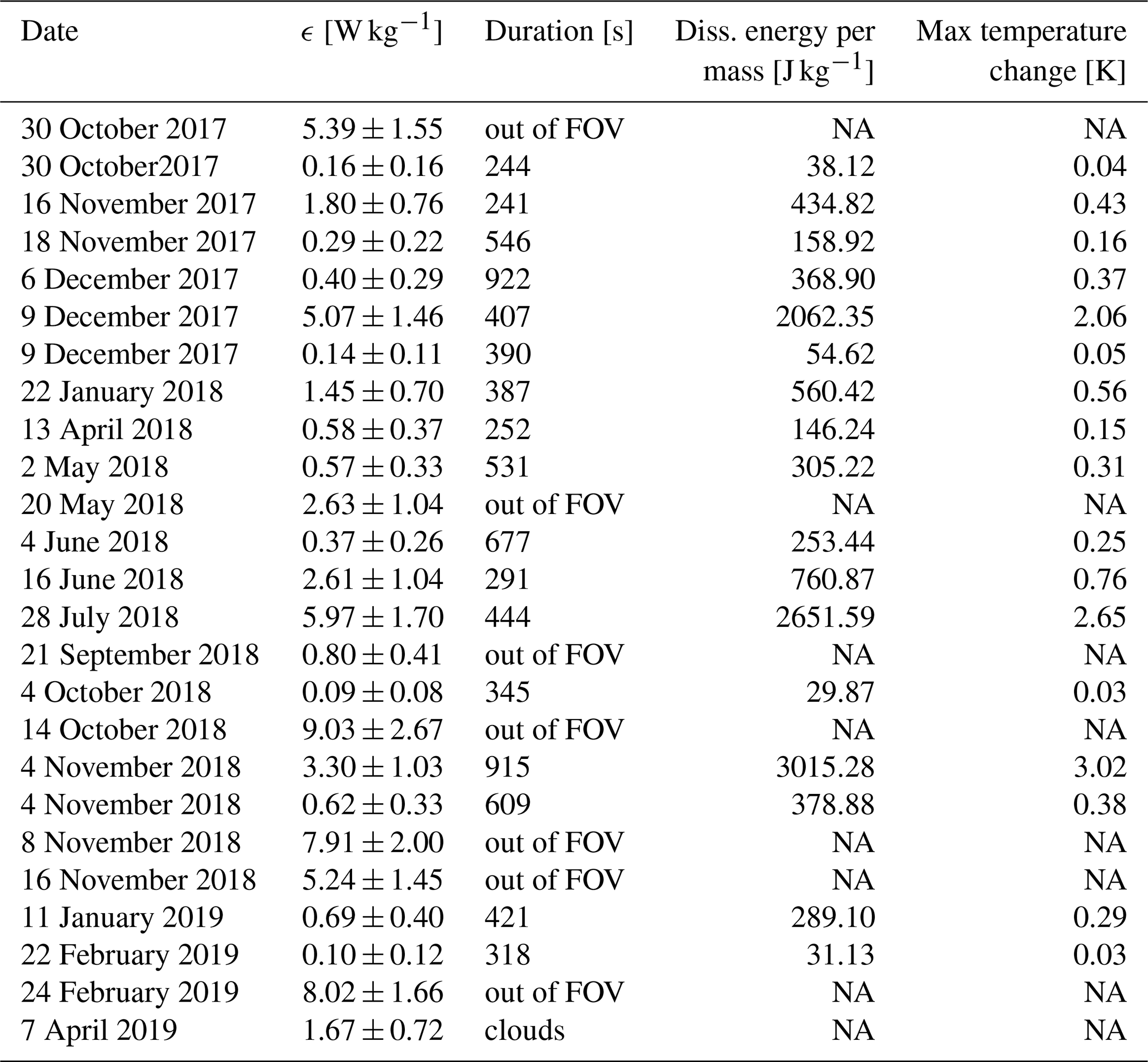
We often observe episodes of turbulence in our image series that exhibit the typical dynamics of vortex formation and quasi-chaotic behaviour. While the identification of wave structures is done automatically by the 2D-FFT, finding turbulent vortices is done by hand. Turbulent eddy formation can be well recognized by eye when viewing the episodes in the dynamical course of a video sequence. However, the combined effect of these vortices having a certain variety of shapes and sizes, being almost invisible in single images without comparison to preceding or successive images, and causing (compared to other features such as wave fronts) rather small brightness fluctuations in the images hampers strongly the application of image recognition algorithms. For the given database, 25 episodes of turbulence with sufficient quality to derive turbulence parameters are found. The dates along with the respective turbulence parameters are summarized in Table 1.

Table 1 Episodes of turbulence observed at OTL and derived parameters from the image sequences. The duration of the turbulence events could not be determined if the vortex was not visible during its entire life span due to being partly outside the FOV (“out of FOV”) of FAIM 3 or covered by clouds (“clouds”). In these cases, we noted the dissipated (Diss.) energy per mass and the maximum temperature change as “not available” (NA).

4 Results

4.1 Statistics of wave parameters

The wave statistics are presented in Figs. 2 and 3. Please note that we a using the word “wave” for all wave-like structures we find in the images. The question of whether these are actual gravity waves is discussed in Sect. 5.

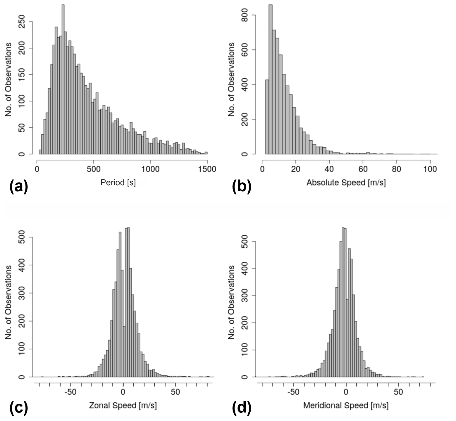
Figure 2 Statistical distribution of observed parameters for wave events with horizontal wavelengths between 48 m and 4.5 km from 26 October 2017 to 6 June 2019 at Otlica, Slovenia. (a) Period; (b) absolute horizontal phase speed; (c) zonal phase speed; (d) meridional phase speed.

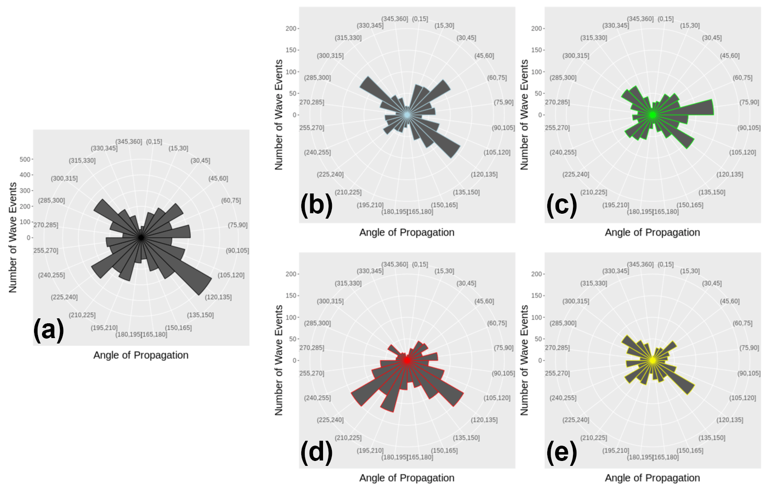
Figure 3 Statistical distribution of observed directions of propagation for wave events with horizontal wavelengths between 48 m and 4.5 km from 26 October 2017 to 6 June 2019 at Otlica, Slovenia. (a) All; (b) winter (December–January–February); (c) spring (March–April–May); (d) summer (June–July–August). (e) Autumn (September–October–November).

Wave periods range from 21 to 1498 s (25 min). The median wave period is 359 s (6 min). The maximum phase speed is 139.8 m s⁻¹ with an average value of 13.3 m s⁻¹ and a standard deviation of 10.3 m s⁻¹. Concerning the zonal distribution, 52.7 % (47.3 %) of the wave events have an eastward (westward) component (consequently no waves with zonal phase speed zero have been observed), and the mean velocity in eastward (westward) direction is 9.4 m s⁻¹ (8.2 m s⁻¹) with a standard deviation of 8.9 m s⁻¹ (7.4 m s⁻¹). We find a small seasonal effect in the distribution of zonal phase speeds: 56.0 % of the waves have an eastward component and 44.0 % a westward component when only considering the winter months December to February, while during summer from June to August 49.5 % of the waves have an eastward component and 50.5 % a westward component. In meridional direction 42.0 % (55.7 %) of the gravity wave events have a northward (southward) component and the mean meridional phase speed is 7.5 m s⁻¹ (9.4 m s⁻¹) in northern (southern) direction with a standard deviation of 7.1 m s⁻¹ (8.7 m s⁻¹). Events with meridional phase speed zero have not been considered for the mean values.

4.2 Wave dissipation

To give an impression of the turbulent dynamics we observe, we present four of our turbulence episodes as video supplement. On 16 November 2017, 02:16 UTC, the turbulent breakdown of parts of an extended wave field can be observed (Video 1 in the Supplement). On 6 December 2017, 00:26 UTC, several fronts seem to be building up and form rotating vortices (Video 2). This can be observed even clearer on 14 October 2018, 17:08 UTC, where the residual movement of turbulent features can be well recognized above the general background movement (Video 3). On 4 November 2018, 19:18 UTC, breaking wave fronts seem to form rotating structures of nearly cylindrical shape, while these are accompanied by other turbulently moving eddies (Video 4).

We estimate the turbulent energy dissipation rate ϵ using Eq. (1). However, in contrast to Chau et al. (2020), who used radar measurements, we only have horizontal information from our airglow imager. Hecht et al. (2021) demonstrate an approach for how to apply Eq. (1) to purely horizontal airglow imager data, which we adapt to our observations in the following. The characteristic length scale L can be read from the images by measuring the size of the turbulent features. The velocity scale is given by the residual velocity v_res of these features. In our observations, they are part of larger instability features, which we assume to be advected by the background wind. We determine v_res by reading the actual velocity of the turbulent features and subtracting the background movement v_bg in the resulting direction. This is exemplarily shown in Fig. 4. The two patches highlighted therein are both moving to the upper right direction but are approaching each other. This helps distinguishing background and residual movement.

Figure 4 Snapshot (01:14:29 UTC) of the turbulence episode from 6 December 2017. Two patches move in the same directions but have different speeds and are approaching each other. While the feature on the right-hand side seems to be advected by the wind (as do the structures in the entire image), the feature on the left-hand side moves even faster and belongs to those structures that creates the impression of turbulent dynamics. The latter patch moves with the residual velocity that is used in Eq. (1) plus the background velocity. The length scale L used in Eq. (1) is given by the size of this feature. This turbulent episode is attached as Video 2 in the Supplement of this article.

As stated in Sect. 3, we found 25 episodes of turbulence that allowed the derivation of L and v_res. Using Eq. (1), the energy dissipation rate is then calculated by $\mathit{ϵ}=\frac{v_{\mathrm{res}}^{\mathrm{3}}}{L}$. The resulting values are shown in Fig. 5​​​​​​​. We assume a general read-out error of ±3 pixels, which corresponds to a distance of ±72 m. Velocities are determined by reading the distance a feature covers within an episode of at least 10 images, which corresponds to a time span of 28 s. Thus, velocities are estimated with an error of ±2.6 m s⁻¹. The arising uncertainties of ϵ are calculated following the rules of error propagation.

The values of ϵ range from 0.08 to 9.03 W kg⁻¹. The median value is 1.45 W kg⁻¹.

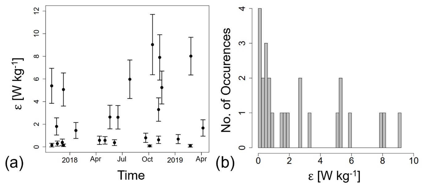
Figure 5 (a) Temporal evolution of energy dissipation rate of observed turbulence events at OTL (see Table 1). (b) Histogram of ε.

Assuming the duration of dissipation being equal to the lifetime of the vortex, the energy dissipation rate can be converted into the amount of dissipated energy per mass. This is only done for those vortices that both form and decay within the FOV. The time intervals of dissipation are between 241 and 922 s (4.0–15.4 min) and can also be found in Table 1. Events are labelled as “out of FOV” or as “clouds” if either the formation or the decay of the vortex cannot be observed. No further analysis is performed for these events.

Multiplying energy dissipation rate and duration of dissipation equals the energy per mass that is released in the turbulent process. We retrieve values between 30 and 3015 J kg⁻¹. Given that the released energy is entirely converted into heat, we can make a rough estimate of the resulting temperature change by assuming isobaric conditions (may be approximately fulfilled due to the stable stratification of the atmosphere and small vertical dimension of eddies) and dividing energy per mass by the specific heat capacity of dry air (10³ J K⁻¹ kg⁻¹). The resulting temperature changes in this work are in the range 0.03–3.02 K (see Fig. 6). All values of dissipated energy per mass and maximum temperature change can be found in Table 1.

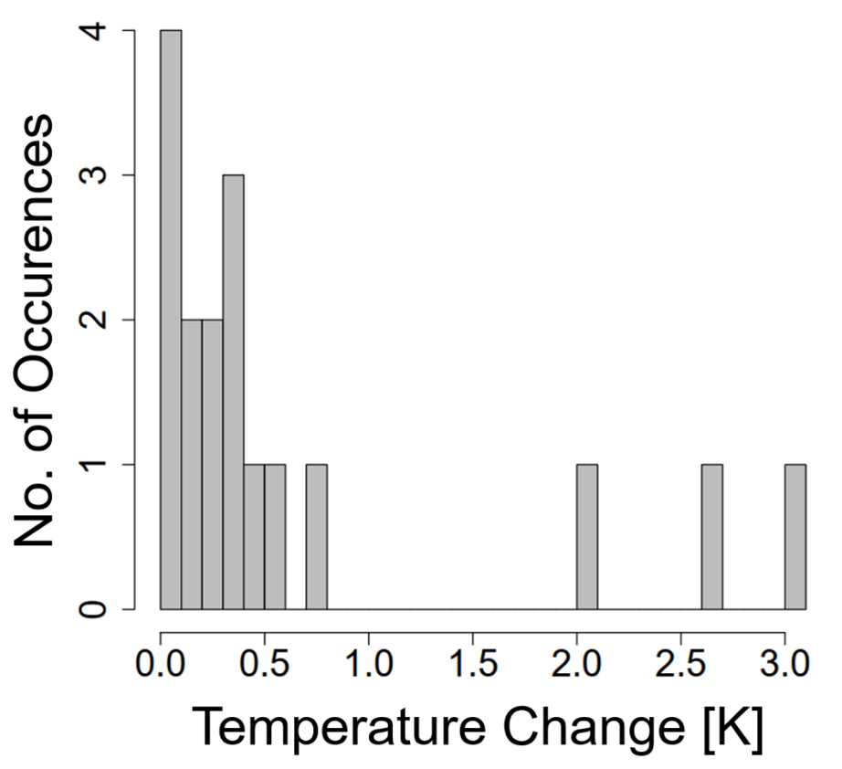
Figure 6 Histogram of temperature change resulting from the observed turbulence events assuming isobaric heating and full conversion into heat.

Since we now have a time series of energy dissipation rate, we can compare them to gravity wave activity in the UMLT above OTL. Parallel to FAIM 3, SWIR spectrometers called GRIPS (GRound-based Infrared P-branch Spectrometer) instruments deliver time series of OH* rotational temperatures derived from the OH(3-1) P-branch (1.5–1.6 µm) at an initial temporal resolution of 15 s. Unlike the general instrument details discussed by Schmidt et al. (2013), the GRIPS 9 at OTL has a reduced aperture angle of 6.2^∘ FWHM, increasing its responsivity to smaller structures. As described in Sedlak et al. (2020), gravity wave activity – the so-called significant wavelet intensity (SWI) – for the periods 6–480 min (period resolution 1 min) can be calculated by applying a wavelet analysis to these temperature time series. The FOV of GRIPS 9 is also located above the Gulf of Trieste and at ca. 30 km distance from the FAIM 3 FOV and has a size of approximately 13 km × 19 km. Since the spectroscopic observations are averaged over the entire FOV, GRIPS is most sensitive for gravity waves with horizontal wavelengths of several hundreds of kilometres (Wüst et al., 2016). The time series of nocturnal SWI is restricted to those nights that exhibited at least one of the turbulence episodes presented above. For each gravity wave period between 6 and 480 min (1 min steps), the correlation between the SWI at the respective period and the energy dissipation rate has been calculated. If there are observations of more than one vortex during one night, the respective energy dissipation rates are averaged to their mean value. The Pearson correlation coefficient and the P value (significance test) are presented in Fig. 7. We find almost no significant correlation for any gravity wave period. Long-period SWI (periods >400 min) shows a slight positive correlation with the energy dissipation rate, which is nearly significant.

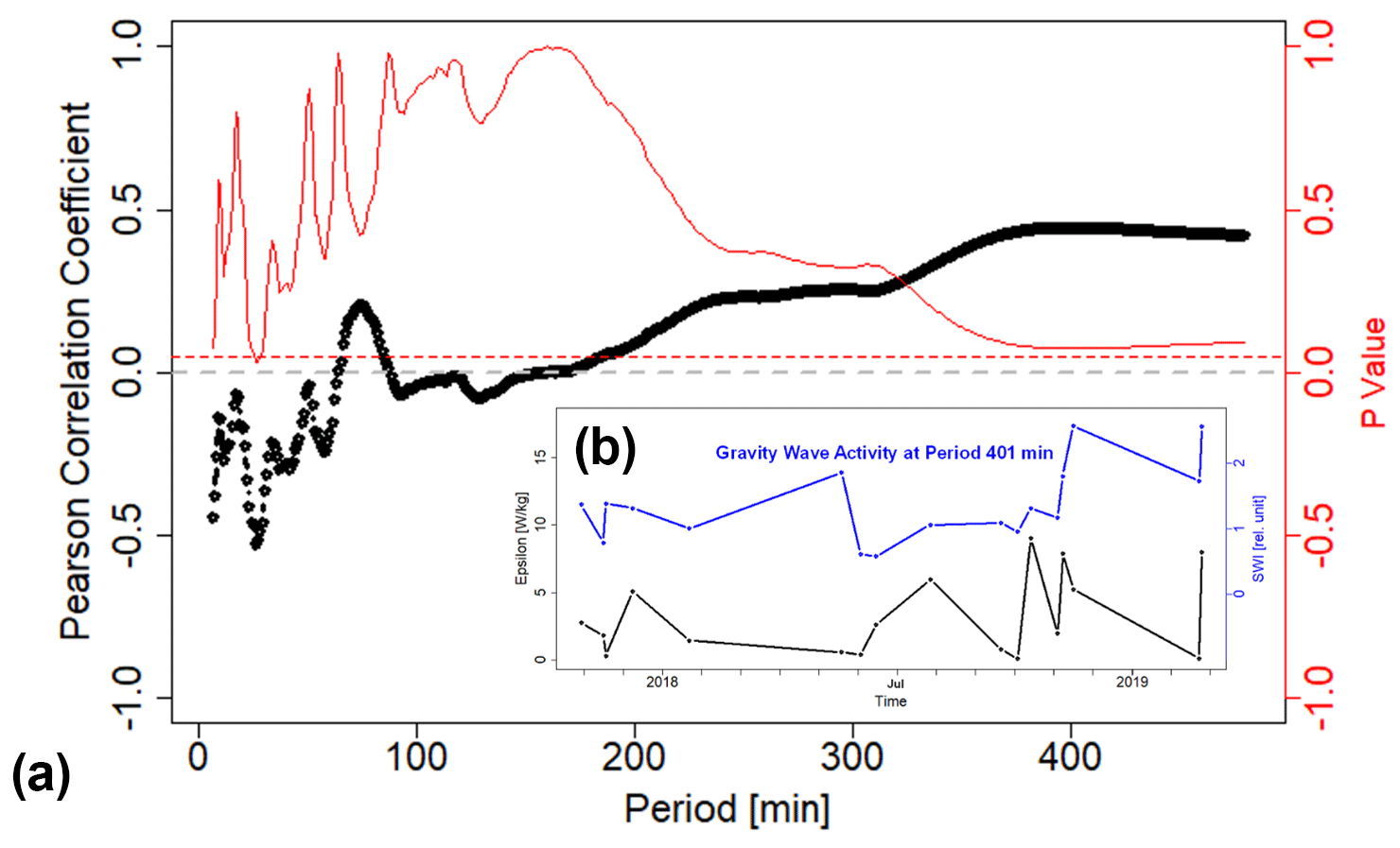
Figure 7 (a) Pearson correlation coefficient (black) between gravity wave activity (SWI) from GRIPS data and energy dissipation rates ϵ from FAIM 3 data above OTL. The P value is plotted in red. For all P values of 0.05 (red horizontal line) or less, the correlation coefficient is considered significant. (b) Comparison of ϵ and the SWI at period 401 min, which is closest to a significant positive correlation in the long-period part of the gravity wave spectrum (Pearson correlation coefficient of 0.45).

5 Discussion

As can be seen in Fig. 3, the wave structures we observed exhibit multiple directions. The strong tendency to the north-eastern direction in summer and to the (south-)west in winter as observed by Hannawald et al. (2019) for medium-scale gravity waves cannot be confirmed for the waves observed here. However, slight tendencies are apparent in Fig. 3. The north-western component these authors observed during winter at Mt Sonnblick in Austria with the FOV being positioned north of the Alps also appears in our data during autumn, winter and spring. During summer we find a conspicuous majority of waves propagating into the southern direction.

The number of waves propagating eastward and westward is almost equal for the entire data set. However, as stated in Sect. 4.1, more waves are oriented in eastward direction during winter, whereas zonal directions are quite balanced during summer. Although the eastward tendency during winter is quite weak, it contradicts the distribution that is expected for gravity waves being created in the lower atmosphere and propagating upward, being subdued to tropospheric and stratospheric wind filtering. The eastward oriented mean wind profile during winter would lead to mainly westward propagating gravity waves reaching the UMLT without encountering critical levels. During summer the stratospheric winds reverse to westward direction, so eastward oriented gravity waves are filtered in the tropopause and westward oriented gravity waves are filtered in the stratosphere (see, for example, Hoffmann et al., 2010; Hannawald et al., 2019).

As we have no accompanying wind measurements in the height of our observations, it is difficult to decide by means of the period whether the wave structures presented in Sect. 4.1 are small-scale gravity waves or instability features. Ca. 63 % of the wave events have an observed period above the BV period (here we used the climatology presented by Wüst et al., 2020); however, these could at least in parts also be Doppler-shifted instability features instead of gravity waves. While the distinction between largely extended wave fields (bands) and small localized wave structures that are related to instability (ripples) is often made at a horizontal wavelength of 10–20 km (Taylor, 1997; Nakamura et al., 1999), Li et al. (2017) remark that even structures with horizontal wavelengths of 5–10 km may sometimes be gravity waves rather than instability features.

If this were true for our small-scale wave structures, they might rather be secondary gravity waves (see, for example, Becker and Vadas, 2018), being generated at greater heights by breaking gravity waves. Secondary gravity waves can either have larger wavelengths and phase speeds than the primary wave if they are created by localized momentum deposition (Vadas and Becker, 2018) or smaller wavelengths and phase speeds if they are induced by the nonlinear flow (wave-mean flow and wave–wave interactions; see, for example, Bacmeister and Schoeberl, 1989; Franke and Robinson, 1999; Bossert et al., 2017). The former type of secondary gravity waves exhibits a rather broad spectrum of wave parameters with horizontal wavelengths longer than 500 km and horizontal phase speeds between 50 and 250 m s⁻¹ (Vadas et al., 2018), resulting in periods longer than ca. 30 min. The wave structures found in this work have smaller horizontal wavelengths, phase speeds and periods and could therefore be more likely related to the latter type of secondary waves created by nonlinearities. However, these small-scale secondary waves are unlikely to propagate large vertical distances due to their small horizontal phase speeds (Becker and Vadas, 2018). They have to be generated at even higher altitudes, i.e., close to the mesopause, to be observable with OH* airglow imagers. Hannawald et al. (2019), for example, deduce from their observations that not only the zonal stratospheric winds but also the meridional circulation in the mesosphere might play a vital role in filtering gravity waves. The meridional mesospheric circulation is oriented southward during summer and northward during winter, being much stronger during summer with ca. 10–14 m s⁻¹ (Yuan et al., 2008). Simulations by Becker and Vadas (2018) show that advection by the background wind determines the direction of a newly created secondary wave. Based on these aspects, the accumulation of southward oriented waves we observe during summer could be a hint for gravity waves being filtered by the mesospheric circulation and generating subsequent secondary waves with shorter wavelengths and periods, which are provided with a southward phase speed due to advection. This theory is also in good agreement with our observed meridional phase speeds: in the above-mentioned velocity range of the summerly meridional mesospheric circulation (10–14 m s⁻¹), meridional phase speeds are southward in 71 % of cases.

However, regarding the small horizontal wavelengths below 4.5 km, it is more likely that the major part of the observations presented in Sect. 4.1 are related to instability features. The quite slow phase speeds (mean value 13.3 m s⁻¹) are one hint for this as typical gravity wave phase speeds accumulate around 40 m s⁻¹ (see, for example, Wachter et al., 2015, and Wüst et al., 2018). If Fig. 2b was the phase speed distribution of gravity waves, it is likely that a majority of them would encounter critical levels somewhere and would not be observable in the OH* layer. The small spatial scales of the wave structures we observe are typical for ripple structures as they were already observed with FAIM 3 (Sedlak et al., 2016). Their short life spans are not excluded by our quality criteria. Tuan et al. (1979) state that oscillations of this type are usually excited at periods of 4–10 min, which would explain the large number of wave events we observe in this period range. Observing ripple structures, it would not be surprising to obtain a certain diversity of directions of propagation. In principle, ripples originating from convective instabilities tend to be aligned perpendicular to the wave fronts of the initial wave, whereas ripples arising from dynamic instabilities form parallel to the initial wave fronts (Andreassen et al., 1994; Fritts et al., 1997; Hecht et al., 2000). However, it has been reported that ripples can be rotated by the background wind and that ripples may even be created by a combination of both dynamical and convective instability (Fritts et al., 1996; Hecht, 2004). Considering the fact that the directional peculiarities of our observed wave events fit well with the expected behaviour of secondary gravity waves, as discussed above, this supports the scenario of the wave structures being ripples from dynamic instabilities of secondary gravity waves, which originate from the stratospheric and mesospheric jet. Capturing structures related to instability is not unlikely, considering the numerous observations of turbulent vortices with the FAIM 3 set-up.

Nevertheless, height-resolved measurements of the horizontal wind would be needed to determine the local wind shear and make a profound statement about atmospheric instability.

It has to be kept in mind that a 2D-FFT was used. Thus, periodic structures are assumed to be stationary, i.e., they extend over the entire image. Faint structures that appear only in small parts of the image (as does, for example, the 550 m wave packet in Sedlak et al., 2016; Fig. 2) would be underrepresented by this analysis.

Measuring the energy dissipation rate in the UMLT is still challenging, and there are only few studies yet. Rocket measurements of Lübken (1997) deliver energy dissipation rates between ca. 0.01 and 0.1 W kg⁻¹ between 85 and 90 km height at high latitudes. Chau et al. (2020) find an energy dissipation rate of 1.125 W kg⁻¹ for their KHI event observed in the summer mesopause and state that this a rather high value compared to the findings of Lübken et al. (2002). Hocking (1999) provides a rescaled overview of earlier values of the energy dissipation rate and these have a maximum magnitude of 0.1 W kg⁻¹. Hecht et al. (2021) derive a value of 0.97 W kg⁻¹ from airglow images of a KHI event. Ranging from 0.08 up to 9.03 W kg⁻¹, the values of energy dissipation rate derived here are higher than reported by other studies. However, the median value of 1.45 W kg⁻¹ is not too far away from the values of Chau et al. (2020) and Hecht et al. (2021). The vortices we observe do not necessarily mark the small-scale end of the energy cascade. It could be possible that the energy is cascaded further to a larger number of smaller eddies that are no longer visible to our instrument. Parallel in situ measurements (e.g., lidar, rockets) could be used to estimate the significance of this effect. Additionally, it has to be kept in mind that – except for the studies of Hecht et al. (2021), whose value is quite similar to the median value of our data – the values compared here arise from different measurement techniques with different horizontal, vertical and temporal resolutions, so the accessible scales are not necessarily identical due to the observational filter effect.

The derivation of the turbulence parameters performed here is challenging due to the blurred shape of dynamic signatures in the OH* layer. The length scale and velocity scale of turbulent features have been extracted manually by measuring distances in the images and calculating distances from pixel values. We tried to quantify the read-out error by providing a measurement uncertainty and minimizing it by repeating the analysis workflow on the same data multiple times. However, using Eq. (1) velocity dominates the length scale due to its power of 3, so ϵ strongly depends on a parameter which is quite difficult to extract from the images. All in all, it seems possible to derive turbulence parameters like the energy dissipation rate from high-resolution imager data.

The values of energy dissipation rate derived here show no significant correlation with gravity wave activity in the period range 6–480 min. Turbulence thus can hardly be related to distinct periods of the gravity wave spectrum with the here-presented data. The slight positive correlation with gravity wave activity at periods larger than 400 min may point to a special contribution of long-period gravity waves to the turbulence events we observe. However, this remains speculative at the current stage of research, since this correlation is beyond the level of significance. A larger database of turbulence parameters and especially observations of period-resolved gravity wave activity at altitudes below will be needed to answer the question of whether all parts of the gravity wave spectrum drive turbulence generation in the UMLT equally.

Assuming that the turbulently dissipated energy is entirely converted into heat, we find temperature changes of 0.03–3.02 K that occur within time spans of 4.0–15.4 min. Marsh (2011) report chemical heating rates in the atmosphere to be around 3–4 K per day. Given that our analysed episodes are typical representatives of turbulent wave breaking, dynamical heating by gravity wave dissipation would deliver the same effect within few minutes at very localized areas in the UMLT as does chemical heating during an entire day for the whole atmosphere.

6 Summary

We present an analysis of small-scale dynamics of instability features and turbulence from OH* imager data acquired between 26 October 2017 and 6 June 2019 at Otlica Observatory, Slovenia. Measurements have been performed with the imager FAIM 3, which has a spatial resolution of ca. 24 m per pixel and a temporal resolution of 2.8 s.

Wave-like structures in the images are systematically identified by applying a 2D-FFT to nocturnal image sequences during clear-sky episodes. All events meeting our persistency criteria were used to derive a statistical analysis of wave-like structures with horizontal wavelengths between 48 m and 4.5 km. The small horizontal scales are a strong hint that these are likely instability features of breaking gravity waves like ripples. We generally find variable directions of propagation, which indicates that these wave-like structures may be mostly created above the stratospheric wind fields. However, a weak seasonal dependency is found: zonal directions of propagation are slightly more eastward during winter and westward during summer. We speculate these to be instability features generated by breaking secondary gravity waves, receiving their zonal direction through advection by the background wind. We find a stronger tendency of southward propagation during summer, which may point to a vital role of gravity wave filtering and excitation of secondary waves and their subsequent instability features by the meridional mesospheric circulation.

Furthermore, we observed and presented OH* imager observations of turbulence with high spatio-temporal resolution. We estimated turbulence parameters from 25 episodes of eddy observations. Following the approach of Hecht et al. (2021), we derived the energy dissipation rates for our observed events by reading the turbulent length and velocity scale from the image series. Our values range between 0.08 and 9.03 W kg⁻¹ and are higher than earlier rocket measurements. The values presented here would cause localized heating of 0.03–3.02 K per turbulence event. The largest of these reach the same order of magnitude as the daily chemical heating rates as reported by Marsh (2011). Given that the observed events are representative of typical processes of gravity wave dissipation, this emphasizes the importance of carefully integrating gravity wave turbulence into climate simulations.

Being able to derive reasonable values of UMLT turbulence parameters from imager data represents an important progress for measurement techniques of atmospheric dynamics. Airglow imagers are much cheaper and more flexible than rockets or lidars. Considering the huge amount of data, artificial intelligence could be used in the future to identify and analyse turbulent episodes.