the Creative Commons Attribution 4.0 License.
the Creative Commons Attribution 4.0 License.
 | 25 Oct 2021
Reconstruction of the mass and geometry of snowfall particles from multi-angle snowflake camera (MASC) images
Jussi Leinonen
Alexis Berne
This paper presents a method named 3D-GAN, based on a generative adversarial network (GAN), to retrieve the total mass, 3D structure and the internal mass distribution of snowflakes. The method uses as input a triplet of binary silhouettes of particles, corresponding to the triplet of stereoscopic images of snowflakes in free fall captured by a multi-angle snowflake camera (MASC). The 3D-GAN method is trained on simulated snowflakes of known characteristics whose silhouettes are statistically similar to real MASC observations, and it is evaluated by means of snowflake replicas printed in 3D at 1:1 scale. The estimation of mass obtained by 3D-GAN has a normalized RMSE (NRMSE) of 40 %, a mean normalized bias (MNB) of 8 % and largely outperforms standard relationships based on maximum size and compactness. The volume of the convex hull of the particles is retrieved with NRMSE of 35 % and MNB of +19 %. In order to illustrate the potential of 3D-GAN to study snowfall microphysics and highlight its complementarity with existing retrieval algorithms, some application examples and ideas are provided, using as showcases the large available datasets of MASC images collected worldwide during various field campaigns. The combination of mass estimates (from 3D-GAN) and hydrometeor classification or riming degree estimation (from independent methods) allows, for example, to obtain mass-to-size power law parameters stratified on hydrometeor type or riming degree. The parameters obtained in this way are consistent with previous findings, with exponents overall around 2 and increasing with the degree of riming.
- Article
(5509 KB) - Full-text XML
- BibTeX
- EndNote


Cloud and precipitation microphysics refer to the interactions and processes that are relevant at the scale of individual particles. Microphysics and microstructure, namely, the distribution of particle properties like size, shape, number density and mass, define together the state and the evolution of clouds and precipitation at this scale (Pruppacher and Klett, 2000). The parametrization of microphysics in numerical weather models has a major impact on how accurately the links within the water cycle are depicted (Thompson et al., 2008; Liu et al., 2011; Morrison et al., 2020). Research on ice-phase precipitation (snowfall) microphysics and microstructure is complicated by the complex geometry of individual or aggregate crystals (see Magono and Lee, 1966; Ford, 2014, for visual examples) and by the multitude of processes influencing the density, size and fall speed of the hydrometeors: riming, aggregation, melting, vapor deposition, sublimation, and secondary ice production, only to cite a few. Not only is the complex three-dimensional structure of snowflakes poorly understood but there is also an active debate on the range of validity and applicability of mass–size relations (Dunnavan et al., 2019; Karrer et al., 2020) as well as on the appropriate shape approximation of snowflakes as oblate or prolate spheroids or ellipsoids (Jiang et al., 2017, 2019; Dunnavan et al., 2019). It seems established that the model of snowflakes as spheroids of constant density is oversimplified and outdated (Dunnavan et al., 2019) as this assumption affects significantly the interpretation or retrievals of active remote-sensing measurements of snowfall (Leinonen et al., 2013; Leinonen and Szyrmer, 2015).
Among the challenges in the field of snowfall microphysics, a key role is played by the difficulty to conduct undisturbed observations of snowflakes in free fall. Garrett and Yuter (2014) underlined how currently used size–fall-speed relations still rely on experiments performed on a limited number of snowflakes (Locatelli and Hobbs, 1974). Particle habits and shapes are even more complicated to study and much of the current knowledge on individual ice crystals is based on controlled laboratory experiments rather than outdoor real-world observations (Takahashi, 2014; Weitzel et al., 2020). The commercialization of a few ground-based instruments designed to collect actual images of falling hydrometeors and estimate at the same time their fall speed has given a noticeable momentum to this field of research. An example is the two-dimensional video disdrometer (2DVD; Kruger and Krajewski, 2002), providing orthogonal silhouettes and speed of falling particles. More recently, accurate and high-resolution depictions of snowflakes could be obtained with imagers like the snow video imager/particle image probe (Newman et al., 2009) or with the multi-angle snowflake camera (MASC; Garrett et al., 2012). The availability of actual images has promoted the development and rapid improvement of several automatic hydrometeor classification techniques (Grazioli et al., 2014; Gavrilov et al., 2015; Praz et al., 2017; Leinonen and Berne, 2020) adapted to the data of these sensors. While the accuracy of the measurements of fall velocity provided by those instruments is often hampered by wind and turbulence (Nešpor et al., 2000; Garrett and Yuter, 2014; Fitch et al., 2021), the added value in terms of microphysical characterization is significant.
Unlike other instruments, MASC captures simultaneously three pictures of falling hydrometeors from three distinct coplanar viewpoints, opening the conceptual possibility to perform a 3D reconstruction of the observed snowflakes. To date, the only documented effort to perform this retrieval has been proposed by the visual hull (VH hereafter) approach by Kleinkort et al. (2017). VH has been shown to produce good retrievals of multi-dimensional shapes from the combination of single-view cameras, especially for a modified version of MASC mounting five cameras instead of three. VH performs an accurate retrieval of volumes, and it does not tackle directly the retrieval of the mass of individual snowflakes, which is one of the focuses and motivations of the method proposed in the present paper. The need to obtain simultaneous measurements or estimates of mass and shape of individual particles has been in fact declared “urgent for the scientific community” by Jiang et al. (2019).
In this article we present a method, based on a generative adversarial network (GAN), to retrieve the three-dimensional distribution of mass of individual snowflakes using as input the two-dimensional triplet of images collected by a MASC. GANs are nowadays finding application in the field of environmental and atmospheric sciences (e.g., Leinonen and Berne, 2020; Leinonen et al., 2021) thanks to their versatility, and their ability to perform 3D reconstruction of images has been already explored, for example, in the medical field (Yang et al., 2017). The GAN presented here is trained on a set of simulated snowflakes (generated using the technique of Leinonen et al., 2013; Leinonen and Moisseev, 2015; Leinonen and Szyrmer, 2015; Karrer et al., 2020) and evaluated on 3D-printed 1:1 scale snowflake replicas repeatedly dropped into the MASC sampling area.
This article is organized as follows. Section 2 describes the MASC, the instrument used in the present study. Section 3 details the methods, data, and the novel mass and shape estimation algorithm. Section 4 is devoted to the evaluation of the retrieval, while Sect. 5 provides examples of applications and potential future studies. Section 6 draws the main conclusions of this work.
The method presented here is built and designed for the data collected by the multi-angle snowflake camera (MASC). We briefly recall here the most important technical characteristics of the instrument and the known limitations, and we refer the interested reader to more detailed literature on the subject at the end of this section.
A MASC is composed of three high-resolution coplanar cameras pointed to a common focal point. Each camera is separated by 36∘ with respect to the next one (rotation around the vertical axis) such that a picture of a given snowflake can be obtained simultaneously at an angle of 0 and ± 36∘. Two infrared (IR) emitter–detector pairs are triggering the cameras and three associated spotlights. The IR arrays are separated vertically by 32 mm, providing in this way an estimate of particle fall velocity. For the data shown here, the MASC system is composed of three 2448×2048 pixels cameras, and the maximum acquisition rate is about 2 Hz (as in Praz et al., 2017).
The data processing steps employed in this study are the same as in Praz et al. (2017), although only a minor part of the information generated is used as actual input of the method described in the following section, while another part can be used to interpret and complement the output (as illustrated in Sect. 5). The preprocessing involves snowflake identification (and matching) in the three images, calculation of geometrical and textural descriptors, image quality evaluation, hydrometeor classification and riming degree estimation.
Although the MASC is a relatively recent instrument, the interested reader can find a fair amount of relevant literature about it. Its measurement principle is detailed in Garrett et al. (2012). Several studies exploited MASC data to investigate geometry and fall speed characteristics of hydrometeors (Garrett and Yuter, 2014; Garrett et al., 2015; Jiang et al., 2019), and others were devoted to hydrometeor classification techniques as in Praz et al. (2017), Hicks and Notaros (2019), and Leinonen and Berne (2020). Recent work tackled the challenge of automatic discrimination of precipitation, wind-blown snow and their mixtures (Schaer et al., 2020). The limitations of the instrument and noteworthy wind-related data degradation issues are well summarized in Garrett and Yuter (2014) and Fitch et al. (2021). Finally, an upgraded version of the MASC equipped with five cameras is described in Kleinkort et al. (2017).
3.1 Generative adversarial networks
GANs, belonging to the family of deep learning techniques (Alom et al., 2019), are generative models that are trained as a combination of two neural networks: the discriminator and the generator. The discriminator is trained to distinguish samples that belong to the training dataset from those that do not, while at the same time the generator is trained to produce outputs that the discriminator considers to be real. This results in the two training processes competing against each other, which is referred to as adversarial training. Since the discriminator is a powerful image recognition network, the generator must learn to produce highly realistic outputs in order to successfully “fool” the discriminator. The generator is able to produce diverse outputs because it is fed random noise as an input, and the generator learns to map the distribution of the noise to the distribution of the input data. In a conditional GAN, both the discriminator and the generator additionally receive a condition as input data; therefore, the generator learns the conditional probability distribution of the input data.
In the original GAN formulation by Goodfellow et al. (2014), the discriminator is a binary classifier, but it was found by Arjovsky et al. (2017) that some of the instability problems of GANs are remedied by reformulating the objective using a dual of the Wasserstein distance of probability distributions. Gulrajani et al. (2017) then combined this approach with a constraint on the gradient of the weights with respect to the training objective; this combination is referred to as a Wasserstein GAN with gradient penalty (WGAN-GP). Given its superior stability with respect to the original GAN, a WGAN-GP is employed in the present study.
3.2 The 3D reconstruction GAN
Our 3D reconstruction GAN, named 3D-GAN hereafter, is formulated as a conditional WGAN-GP, where the desired data are the 3D structure of the snowflake, and the condition is a set of three binary images (silhouettes) captured from the angles at which the MASC sees the snowflake. The objective for the generator is thus to generate a 3D structure that the discriminator considers as appropriate for the image triplet.

Figure 1Illustration of the architectures of the (a) generator and (b) discriminator of the GAN.
The generator network is shown in Fig. 1a. The inputs are three snowflake silhouettes of 128×128 pixels. The first part of the processing passes the inputs through a series of residual downsampling blocks followed by a fully connected layer, resulting in a set of descriptors for each image. Following the “Siamese network” approach (Chicco, 2021), this step is implemented using the same weights for each image. The descriptors are then concatenated and processed through several fully connected layers, resulting in a set of descriptors for the image triplet. At this stage, the noise is also included in the model by multiplying the input of the second fully connected layer with the noise vector. These descriptors are then passed through one more fully connected layer to produce 2048 variables, which are then reshaped to thirty-two 3D feature maps of pixel size. In the final stage of processing, the 3D feature maps are passed through upsampling blocks, eventually producing a 3D grid of 32 × 32 × 32 grid volume elements (voxels). The size of the produced grid was selected as a compromise between resolution and computational requirements.
The inputs to the discriminator (Fig. 1b) are a 3D grid (either from the training dataset or from the generator) and a triplet of images. The images are processed to descriptors using a Siamese network in a manner identical to the generator. Meanwhile, the grid is passed through a set of downsampling 3D convolution blocks, the result of which is flattened into descriptors. The descriptors for both the 3D grid and the images are processed through multiple fully connected blocks. The descriptors for the grid and the images are then combined by multiplying them with each other. The result of this is passed through more fully connected blocks, eventually producing a single scalar as the discriminator output.
While the silhouettes are binary images, the value of each voxel in the 3D grid is proportional to the average density of the ice–air mixture within that voxel, scaled such that the mean density of the nonzero voxels is approximately 1. It is therefore possible to compute the snowflake mass from the outputs of the GAN. We however found that we can achieve better mass estimation with a separate neural network trained specifically to predict the mass. For this, we used a network architecture similar to that of the discriminator (Fig. 1b), except without the 3D grid input and processing branch. This network gives us the total mass m; to estimate the mass mi in each voxel i in the 3D grid output of the generator, we scale the voxel value as
where yi is the generator output at voxel i.
3.3 Training
Training the 3D reconstruction GAN requires large training datasets of 3D structures and MASC imagery. As it is extremely difficult to accurately map the 3D structure of a snowflake, such datasets are currently not available from measurements of real snowflakes. Thus, we train the GAN using synthetic observations from modeled snowflakes created with the snowflake generation model described in Leinonen et al. (2013), Leinonen and Moisseev (2015), and Leinonen and Szyrmer (2015). This model creates volumetric 3D models of snowflakes and is capable of modeling single crystals, aggregation and riming. The degree of riming is indirectly prescribed by the liquid water path (LWP, in kg m−2) parameter (Leinonen and Szyrmer, 2015). The generated snowflake models are defined by a set of volume elements of 40 µm size, each either entirely filled with solid ice of density ρice = 917 kg m−3 or empty. In order to create a training set, snowflakes are generated by randomly selecting a few input parameters. To cite the most important, LWP varies from 0.0 to 2.0 kg m−2; the number of monomers varies between 1 and 50; the monomer type varies among dendrites, needles, rosettes, plates, and columns; and the riming process is chosen as either occurring at the same time with respect to aggregation (simultaneous) or only once aggregation is completed (subsequent). For each snowflake generated with the model, we calculated the silhouettes that would be seen by the MASC from the three different camera angles; the silhouettes were artificially blurred by a randomized amount to simulate conditions where the snowflakes are out of focus.
In order to fully utilize the 3D grid and the projection image in the training process and at the same time operate with data of fixed dimensions, the voxels and the projection pixels can correspond to different physical sizes for different snowflakes. Thus, for example, a snowflake of 5 mm maximum dimension would have a grid element size of approximately 5 mm 32 = 0.156 mm and a silhouette pixel size of approximately 5 mm 128 = 0.0391 mm.
The training samples of the GAN are loaded from data files that contain, for each snowflake, the following: the 3D grid, the grid voxel size, 12 simulated projection silhouettes and the projection pixel size. The 12 silhouettes comprise four image triplets; the images in each triplet are 36∘ apart corresponding to the MASC camera separation, while the four triplets are spaced 90∘ from each other. When training the GAN, we increase sample diversity by selecting one of the four triplets at random for each training sample and training step and then rotating the grid correspondingly. We also randomly apply mirroring for further data augmentation.
As mentioned above, we adopt the approach of using a model instead of real observations in the training process out of necessity, while acknowledging that it has a number of potential drawbacks and uncertainties:
-
The model algorithms may not be representative of the physics of real snowflake formation.
-
Although the model can accept any input parameters, the distribution of the model parameters may not match that of real conditions in nature.
-
The simulation of the image formation is not necessarily accurate.
-
By using the silhouettes instead of the grayscale images captured by the real MASC, we lose the texture information contained in the real MASC images.
For the first point, regarding the realism of the physics of the model, we note that although the model does not implement a fully physical simulation of snowflake formation, it has been found to produce realistic mass–dimensional relations of both unrimed (Leinonen and Moisseev, 2015) and rimed (Leinonen and Szyrmer, 2015) snowflakes, and it has been used successfully for modeling snowflake microphysics (Seifert et al., 2019) and remote-sensing signals from snowflakes (e.g., Leinonen et al., 2018; Tridon et al., 2019).
To mitigate the second issue, we forced the distribution of parameters closer to that found in nature using the following strategy. First, we identified a selection of morphological image features that Praz et al. (2017) found important for identifying snowflakes, which did not use texture information and therefore could be calculated also for the silhouettes. We then extracted these features from the dataset by Praz et al. (2017), collected in Davos, Switzerland, during 2016–2017. We excluded the particles classified as “small particles” by Praz et al. (2017), as their size does not allow for any shape recognition or significant variability in the descriptors, and computed principal component analysis (PCA) of the feature distribution on the rest of the population. This excludes particles with maximum dimension roughly lower than half a millimeter. We kept the three most important PCA components, sorted in order of explained variance. Then, while generating snowflakes, we applied a realistic range of parameters such as snow crystal type, number of crystals per aggregate and amount of riming, and we calculated the same features and PCA components. After generating a large number of crystals, we then accepted the generated snowflakes to the final dataset only when they made the distribution of the PCA components for the generated snowflakes closer to that of the real snowflakes, rejecting the others. Thus, we obtained a distribution of snowflake samples that is close to real ones at least in terms of visual descriptors. After this filtering step, the final training set included 20472 samples.
For the third issue, we attempted to simulate the main features of image formation such as randomly blurring the images to simulate situations where they are out of focus. The primary manner in which we attempted to determine if our simulation of the MASC silhouettes is adequate was to use MASC observations of artificial snowflakes 3D-printed from our models, thus using the real MASC rather than a simulation to produce the images. This method is far too labor-intensive and expensive to create large training datasets, but we use it for evaluating the model, as described in Sect. 4.
As for the fourth issue, we accept the lack of texture identification as a current shortcoming of the model. This is unfortunate because the availability of high-resolution texture is one of the greatest advantages of the MASC; however, the radiative transfer of light inside snowflakes is highly complicated, and to our knowledge, no simulation tools exist that could be used to accurately model it and thereby generate proper simulated 2D images from our 3D models, which additionally does not provide surface properties of ice, such as roughness. On the other hand, using only the silhouette images may make our approach easier to adapt to silhouette-only instruments such as the 2DVD.
4.1 Experiment with snowflake replicas
In order to evaluate the performance of 3D-GAN with real MASC data, we used a set a snowflakes printed in 3D. The snowflake shape models were computer-generated with the technique described in Sect. 3.3.
The printer used to generate the particles is a Nanoscribe Photonic Professional GT+ (PPGT+),1 and the material used is a polymer (IP-Q) supplied by Nanoscribe (Bagheri and Jin, 2019). Once polymerized, the material is similar to polymethyl methacrylate (PMMA). The resolution used to generate the flakes is the 3D laser spot size of 1.5 µm diameter (horizontal plane) and 8 µm height (vertical axis).
A few noteworthy limitations set the boundaries of what we could achieve with this approach:
-
The maximum dimension of the printed snowflakes is in the range of 3–5 mm. Smaller snowflakes could not be practically manipulated and larger ones could not be printed.
-
We could not successfully generate completely unrimed particles (LWP = 0 kg m−2) as they resulted in structures too fragile to be manipulated without breaking.
-
Lightly rimed particles sometimes suffered damage while being handled in the MASC measurement area and could thus be used only for a limited number of times.
Table 13D-printed snowflakes used for the evaluation of the 3D reconstruction.
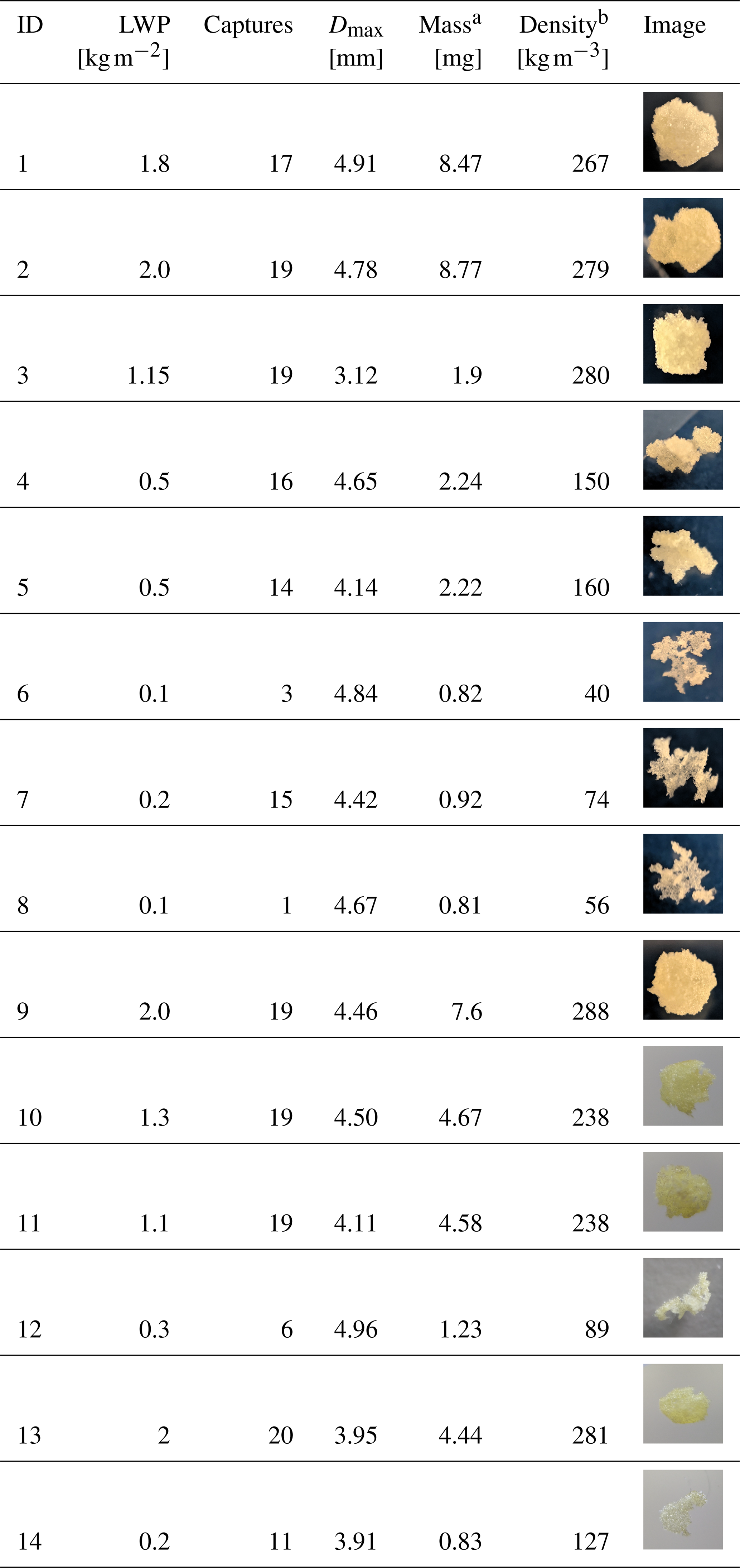
a This is the (ice) mass of the simulated snowflake and not the actual mass of the (polymer) replica. b Calculated using the volume of the convex hull.
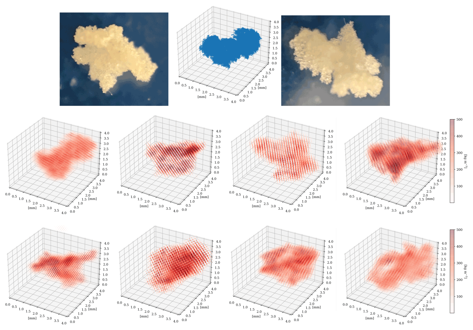
Figure 2Example of the reconstruction outcome obtained while releasing eight consecutive times the same snowflake replica in the MASC measurement area. Top row: actual photos of the replica and a pseudo-3D representation (every blue point represents a voxel filled with ice). Bottom rows: reconstructions obtained with 3D-GAN. Every point is color-coded according to the density (ice mass content) of each voxel.
Fourteen printed snowflakes were used in the evaluation; an overview of their characteristics is shown in Table 1. We dropped each particle several times through the MASC measurement, and after discarding physically damaged particles, a total of 198 MASC triplets (and, accordingly, 198 GAN reconstructions) were obtained. Although a larger population of printed snowflakes would be desirable, we believe that, given the abovementioned limitations and technical difficulties, this training sample is a good starting point, including various snowflake habits as well as different riming degrees. Because the reconstruction is based on the silhouette of MASC images, it follows that, for particles of irregular shape and size, the reconstructed output will vary to a certain extent with the orientation of the falling replicas. This is illustrated in Fig. 2 where one can observe how the reconstruction output varies over several consecutive experimental runs. At the same time, we expect also the reconstruction performance to vary: from some angles the particle may be easier to reconstruct than from others; thus, we performed multiple experiments with the same particles. An additional source of uncertainty may come from the fact that printed snowflakes are not made of ice: their color and optical properties may be different with respect to actual snowflakes. We assume this aspect to be of negligible importance in our case, because only silhouettes are used as input.
4.2 The 1D descriptors
A first evaluation of the ability of 3D-GAN to reconstruct realistic snowflakes can be obtained by looking at one-dimensional descriptors. We selected for this purpose the total snowflake mass m, gyration radius rg, maximum size Dmax and volume of convex hull V𝘾𝙃; Dmax and V𝘾𝙃 are geometric quantities that define exactly the spatial extent of a snowflake. However, the mass distribution of the GAN output is continuously varying; therefore, it is not straightforward to define the exact boundaries of a hydrometeor. The way we tackled this limitation and obtained exact estimates of size and volume is detailed in Appendix A. The evaluation of the descriptors discussed in this section is also summarized in Table 2.
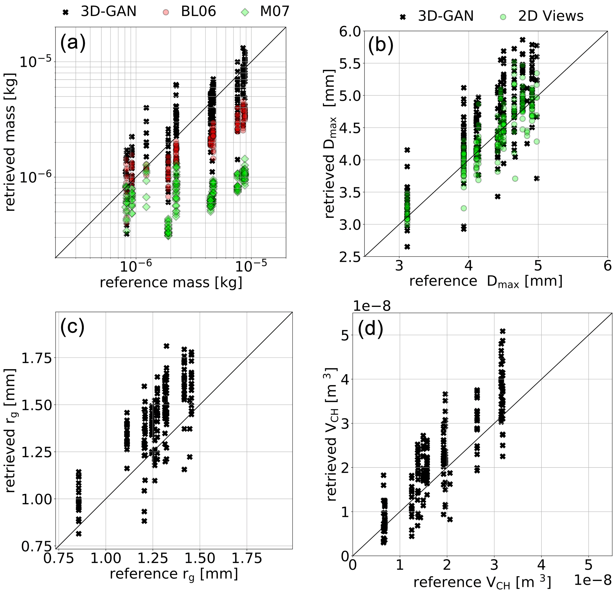
Figure 3Scatterplot of reference (3D-printed replicas) and reconstructed characteristics of the snowflakes used in the evaluation. (a) Mass, (b) Dmax, (c) rg and (d) V𝘾𝙃. For the mass we display 3D-GAN reconstructions as well as mass–size reconstructions by Matrosov et al. (2007) (denoted ML07) and Baker and Lawson (2006) (denoted BL06). M07 and BL06 are calculated on individual MASC views, and the mean value over the three views is shown here in each marker. For Dmax, the estimation obtained using the 2D MASC images is highlighted in green.
Table 2Summary of root-mean-square error (RMSE), normalized RMSE (NRMSE, normalized on the mean value of reference data) and mean normalized bias (MNB) resulting from the comparison with the 3D-printed snowflake replicas.

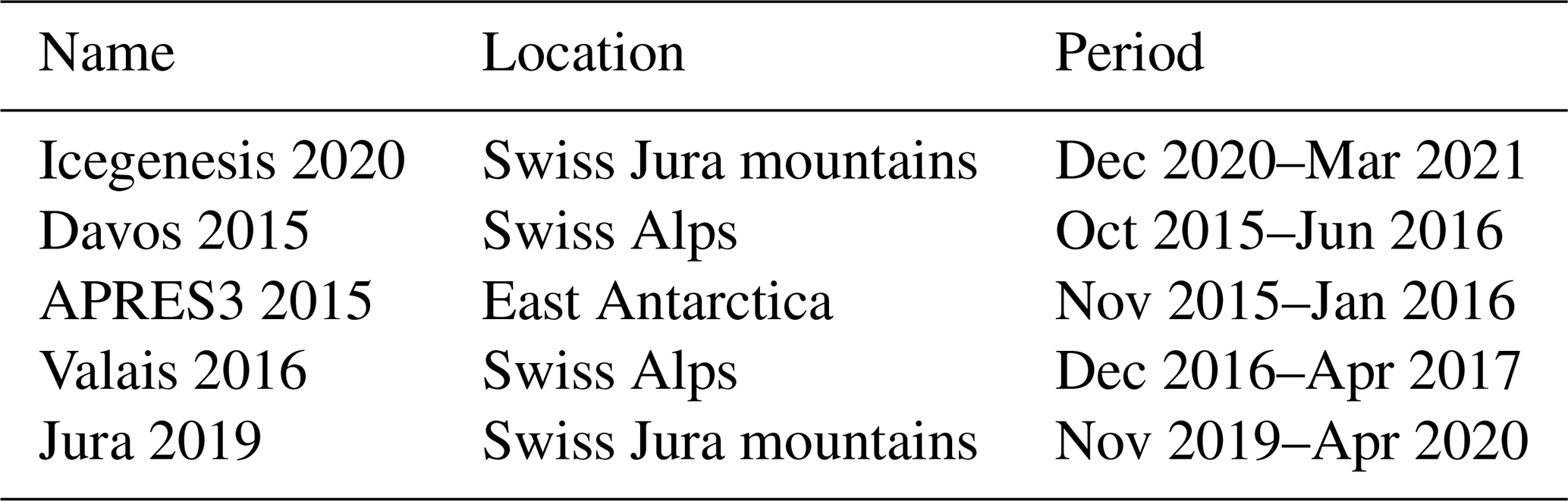
Table 3List of field installations of the MASC instrument, for which data are shown in Figs. 6 and 5.
4.2.1 Mass estimation
Mass estimation is a major added value of the proposed method or at least, in response to the current needs of the scientific community (Jiang et al., 2019), a readily usable product. Figure 3 shows that mass is overall well reconstructed. As a reference, 3D-GAN reconstruction is compared with the methods by Matrosov et al. (2007) (denoted M07) and Baker and Lawson (2006) (denoted BL06). ML07 and BL06 are retrieval formulas designed for two-dimensional images, and we use them here as a benchmark. A large number of mass–size relations exist in the literature, either fine-tuned for specific types of crystals, aggregates, and riming degree (e.g., Leinonen and Moisseev, 2015; Karrer et al., 2020) or obtained by combining the information of several sensors in dedicated field campaigns (e.g., von Lerber et al., 2017). M07 and BL06 are chosen because, like 3D-GAN, they do not require prior knowledge about hydrometeor type and can be readily calculated from the 2-D views of the MASC from silhouette-type images without exploiting textural information. M07 is an adaptive mass–size relation where the exponent and prefactor take different values as the particle dimension (Dmax) increases, and it is a relation in principle valid for unrimed snowflakes. BL06 includes more advanced geometrical considerations, and it uses the maximum dimensions in two orthogonal directions, projected area and perimeter.
The 3D-GAN method largely outperforms both of these estimation approaches, as summarized in Table 2. The normalized root-mean-square error (NRMSE) is roughly 40 % for 3D-GAN, 70 % for BL06 and 103 % for M07, while the mean normalized bias (MNB) is close to 10 %, −40 % and −72 %, respectively. BL06 is able to provide better estimates than M07, although they are both affected by significant negative biases that become mostly evident for the heaviest snowflakes. In our evaluation dataset, the snowflakes having the largest mass are also the ones with the highest degree of riming (see Table 1). In this sense, 3D-GAN shows its ability to indirectly infer the riming degree and the related increase of mass by exploiting the information embedded in the silhouettes. At the same time, heavily rimed particles have more regular shapes and thus represent a less complex geometrical challenge for 3D-GAN. With this in mind, it is also not surprising that BL06, which includes more information on particle geometry and compactness, outperforms a simple mass–size relation as M07.
4.2.2 Geometry estimation
We evaluate here two geometrical quantities: Dmax and V𝘾𝙃 (Fig. 3, bottom panels). Both quantities are reconstructed in a satisfactory manner, with NRMSE of 12 % and 35 %, respectively, and MNB of 7 % and 19 %. The estimation of Dmax is compared with what can be achieved using individual 2D images, selecting the maximum of the three estimates of Dmax, one for each camera view, as, for example, in Praz et al. (2017). Dmax is slightly better reconstructed using the 2D images directly due to the fact that the 3D-GAN mass distribution output varies smoothly, and the exact boundaries can only be approximated with the approach detailed in Appendix A. The retrieval of Dmax from 2D images is practically unbiased, a result in itself interesting for MASC users. Riming has no major impact on the quality of Dmax, while it does affects the retrieval of V𝘾𝙃: particles with LWP greater than 1 are overall better reconstructed (improvements of 15 % in terms of NRMSE while no significant differences in terms of bias, not shown). It is not surprising that heavily rimed particles are better reconstructed in terms of geometry, because their geometry is significantly less complex. In Kleinkort et al. (2017), the performance of the VH reconstruction algorithm for what concerns volume reconstruction (using a standard three-camera MASC) is quantified to be 27 % in terms of absolute error, for a simple spherical test object. The mean absolute error of 3D-GAN for all the printed replicas, thus for significantly more complex shapes, is 30 %. If only heavily rimed particles, thus less complex shapes, are considered (LWP > 1 kg m−2), the error is further reduced down to 26 %. The 3D structure of even heavily rimed particles is certainly more complex than a sphere; thus, it is reasonable and conservative to assume that 3D-GAN performs at least as good as VH for what concerns volume reconstruction, with the significant added value to provide at the same time an estimate of mass m.
The effect of the smooth variation of mass of the 3D-GAN output, without sharp edges, is evident when looking at the gyration radius, rg (Fig. 3), defined in this case as
where N is the number of voxels, is the distance of each voxel with respect to the center of mass of the snowflake and mi is the voxel mass content. rg is overestimated by 3D-GAN (overall by 13 %), indicating that the mass contents of the reconstructed snowflakes have a larger spread around the respective centers of mass in comparison to the structure of the reference snowflakes.
4.3 The 3D mass distribution evaluation
With the evaluation setup described above, the 3D distribution of mass is available. In principle this allows one to compare the reconstructed and reference snowflakes with a voxel-by-voxel approach. Although this 1:1 comparison is undoubtedly ambitious and not straightforward, it is worth it to show here some results in this direction. There are two main preliminary issues to be considered:
-
The orientations of the reconstructed snowflakes depend on the orientation of the printed replicas themselves, as they were falling in the MASC measurement area. The orientation of the reference model is instead fixed.
-
The grid resolution of reference snowflakes is fixed at 40 µm, while the grid resolution of the GAN output varies from flake to flake, as mentioned in Sect. 3.3, and it is generally lower (100 µm or more).
In order to address the first point, a preliminary alignment of each snowflake pair (reconstructed vs. modeled reference) is performed. The snowflakes are considered point clouds, and their best alignment is found with the (rigid-body) point cloud alignment technique implemented in the OPEN3D package by Zhou et al. (2018). The second issue, grid resolution, is tackled by computing voxel-by-voxel performance indicators of mass distribution at various grid resolutions, by first downscaling the data of both snowflakes into a common grid.
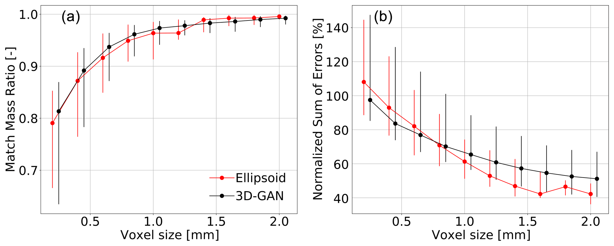
Figure 4Distribution of matched mass ratio (MMR) (a) and normalized sum of errors (NSE) (b) values as a function of the grid volume size at which the evaluation is conducted. Median values over the evaluation sample are indicated by the markers, while the vertical lines overlap the 25th–75th percentile range. An artificial horizontal displacement is added to the data series to enhance readability. The reference method (Ellipsoid) corresponds to an optimal ellipsoidal fit of the reference snowflake with perfect mass match, as described in the text.
Several performance descriptors can be used to evaluate the reconstruction in terms of overlap or quantitative error. We can define here the following two descriptors. Given a pair of three-dimensional snowflakes, one being the 3D-GAN reconstruction and one the reference, let the matched mass ratio (MMR) be
where ΔV is a given voxel size (resolution of the regular grid), and () is the content of mass of the ith voxel of the GAN reconstructed snowflake (reference true snowflake). m3D-GAN (mREF) is the total mass, invariant across scales, of 3D-GAN (reference) snowflake, and N′ defines the set of voxels where the mass content is both nonzero for the GAN and the reference. MMR varies between 0 (worse) and 1 (best), and it evaluates how well the mass of the reconstructed snowflake and the mass of the reference overlap, independently of whether the total mass itself is correctly estimated. A MMR close to 1 indicates that as a whole the combined mass of the two snowflakes occupies the same voxels. A second, significantly more severe and quantitative, indicator is the normalized sum of errors (NSE):
where M is the entire set of voxels where the mass content of 3D-GAN or the reference is nonzero. NSE does not allow for error compensation, and it can in principle be as low as 0 % only if the estimate of total mass of the GAN is perfect.
Figure 4 illustrates the behavior of MMR and NSE across scales. The distribution of mass is overall well matched (mean MMR above 0.8), while the sum of individual errors accumulates, in terms of mean NSE, from 100 % to about 50 % over the range of grid scales. It must be underlined, however, that (i) the best achievable results of NSE are limited to a minimum mean NSE of about 40 %, due to the error in the mass estimation itself, and (ii) the alignment of the two objects is assumed to be optimal. No real adversarial method exists to compute the 3D mass distribution of snowflakes from MASC images, so we decided to show a comparison with an idealized reference as illustrated in the red curves of Fig. 4. This reference corresponds to an ellipsoidal approximation of the reference snowflake with two major competitive advantages with respect to 3D-GAN:
-
The ellipsoid is fitted directly on the original 3D model of the reference snowflake, and not from the MASC captures. The orientation and overlap is thus optimal and no complications and uncertainties due to the realization of an actual measurement can play a role here.
-
The density of the ellipsoid is adapted in order to perfectly match the total mass of the reference snowflake.
The Ellipsoid method is an idealization of the best possible approximation of the snowflakes by means of an ellipsoid of constant density, thus in principle largely superior to any ellipsoidal approximation that can be obtained using actual MASC measurements. The performance of 3D-GAN is close to the one of this idealized retrieval both in terms of MMR and of NSE across all the scales, and most importantly, it is superior at the small scales: up to about 1.25 mm for MMR and up to 0.75 mm for NSE. Regarding NSE, as the scale of the comparison approaches the dimension of the snowflake, the ellipsoid approximation obviously exploits the advantage of “knowing” the exact total mass. Given the idealized nature of the benchmark and the complexity of the retrieval itself, we consider the performance of 3D-GAN satisfactory.
The information provided by 3D-GAN is an important complement to what can be calculated or retrieved from MASC data (e.g., size, shape, complexity, orientation, hydrometeor type or riming degree, as in Praz et al., 2017). We would like to provide the reader with examples and suggestions about possible applications and future research directions that could benefit from the output of 3D-GAN. We consider the retrieval of mass an immediate added value of 3D-GAN and we apply this retrieval here to datasets collected in the past years at various geographical locations. We focus here exclusively on snowfall data, and blowing snow images have been removed using the classification scheme by Schaer et al. (2020).
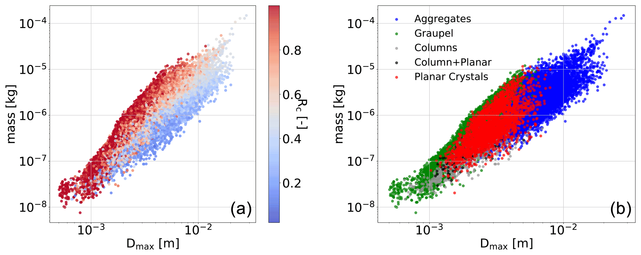
Figure 5m(Dmax) scatterplots for the data of a field campaign, named Davos 2015, which took place in the Swiss Alps in 2015 and 2016. (a) Data are color-coded according to riming index Rc by Praz et al. (2017). (b) Data are color-coded according to the hydrometeor classes, also by Praz et al. (2017).
The availability of both mass and size estimates can be used to construct m(Dmax) relationships using the measurements of a single instrument, the MASC. These relations can then be stratified according to the identified hydrometeor type or as a function of the apparent riming degree, taking advantage of previous work in this direction (Praz et al., 2017). An example is shown in the scatterplots of Fig. 5, for data collected in Switzerland in 2016 and 2017. The same dataset is color-coded according to the apparent riming degree Rc (0 being unrimed particles and 1 fully developed graupel) and according to the classified hydrometeor type. Keeping in mind that 3D-GAN does not have access to textural information other than binary particle silhouettes, it is reassuring to observe in these plots several features that make physical sense. For example, for a given particle maximum size, the riming degree increases the mass content; graupel has the largest mass content (at a given size) while columns the lowest, except for the largest observed sizes that can only be reached by aggregate snowflakes.
Table 4Values of the parameters of the relation m = estimated on the datasets of different field campaigns for various degrees of riming. m is estimated with 3D-GAN, while Rc is the normalized riming index as in Praz et al. (2017), averaged over the three camera views. Dmax is the maximum dimension obtained from the triplet of images of the MASC.
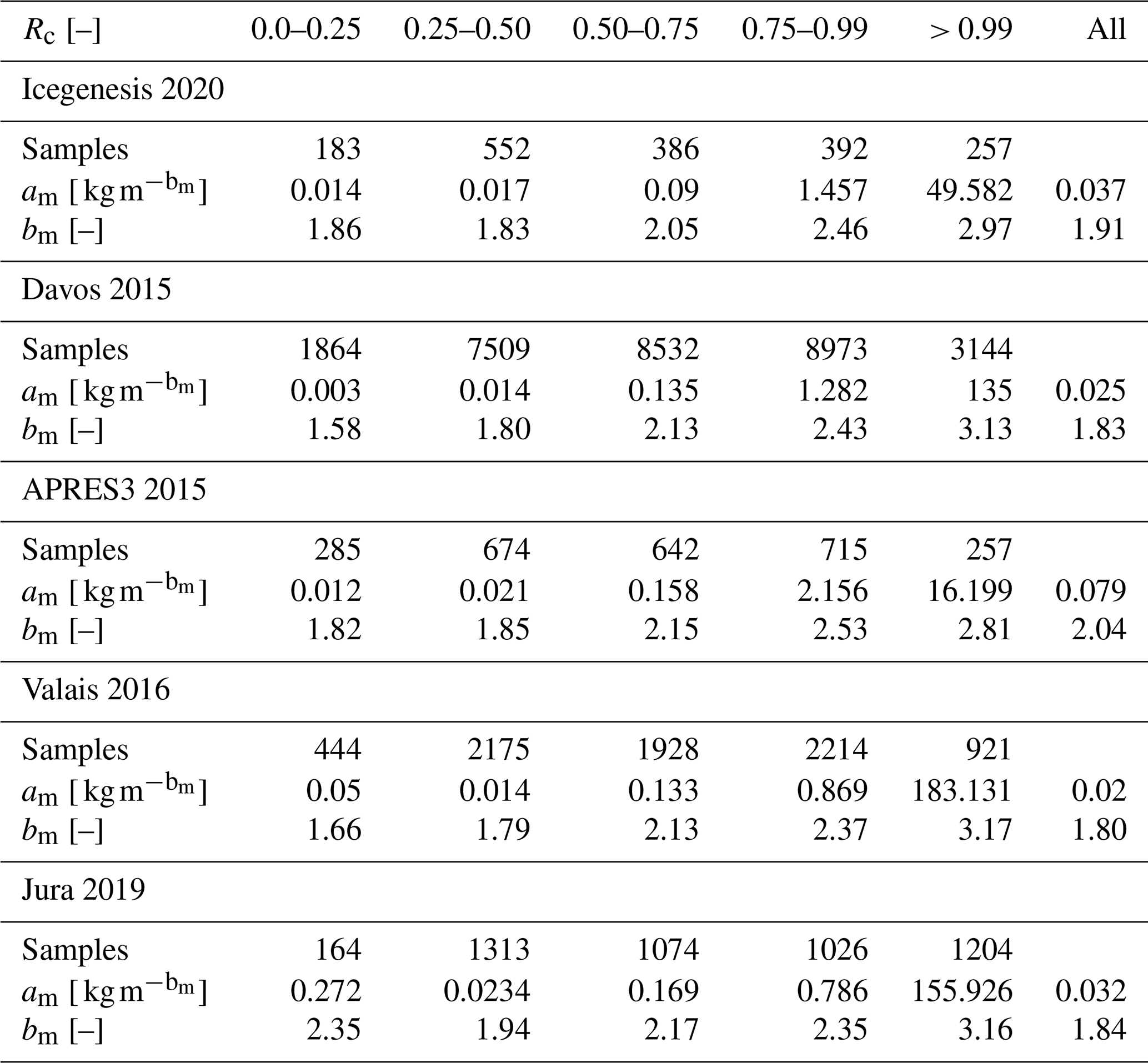
Table 5Values of the parameters of the relation m = estimated on the datasets of different field campaigns for various hydrometeor types. m is estimated with GAN-3D, while the hydrometeor type is obtained with the method by Praz et al. (2017). Dmax is the maximum dimension obtained from the triplet of images of the MASC.
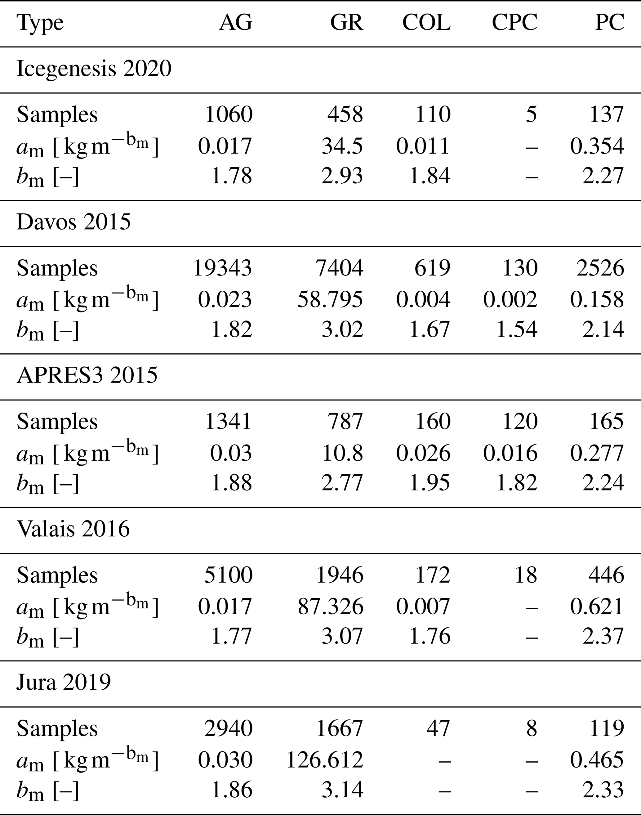
AG: aggregates, GR: graupel, COL: columns, CPC: combination of planar crystals and columns, PC: planar crystals. Results are reported only if at least 80 samples are available.
Tables 4 and 5 provide the parameters of the m(Dmax) power laws calculated for various field campaigns conducted in the Alps and in Antarctica over several years. While an in-depth microphysical interpretation of these results and their differences linked to season and geographical location is beyond the scope of this study, it is worth it to briefly discuss these results and hypothesize how they will be useful to support future research in this direction. Considering the entire datasets of individual field campaigns, values of bm between 1.80 and 2.04 are obtained, in agreement both with studies based on multi-sensor field measurements (e.g., von Lerber et al., 2017, and references therein) and on simulations (Leinonen and Szyrmer, 2015; Karrer et al., 2020). Especially the work by von Lerber et al. (2017) provides bm values also lower than 1.7 and as low as 1.5, as occasionally estimated also by us. Other studies report bm always larger than approximately 1.7 (Mason et al., 2018), 1.9 (Karrer et al., 2020) or 2 (Leinonen and Szyrmer, 2015).
The estimated prefactors am reproduce well the range of values that are documented in the literature.2 In cgs units, the values listed in Tables 4 and 5 span roughly between 0.001 and 0.04 g cm. This range of variation is similar to von Lerber et al. (2017). Also Mason et al. (2018) report values in this range but occasionally higher: up to 0.08 for lump graupel and larger than 0.1 only for hail or solid ice spheres. Leinonen and Szyrmer (2015) obtain a maximum am value of approximately 0.09 g cm but only for a model aiming to reproduce the growth by riming of frozen droplets rather than ice crystals (called rime growth).
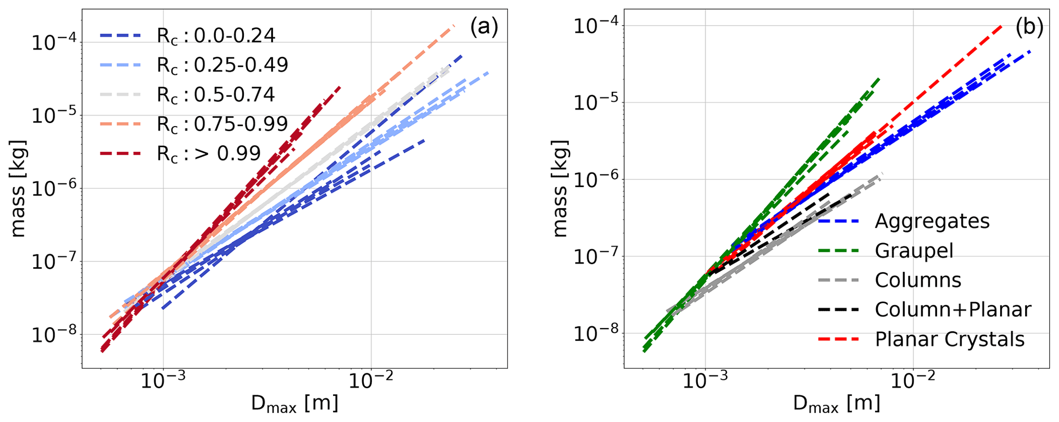
Figure 6m(Dmax) power law relations for the data of various field campaigns, as listed in Tables 4 and 5. (a) Data are color-coded according to riming index Rc by Praz et al. (2017). (b) Data are color-coded according to the hydrometeor classes, also by Praz et al. (2017). Different curves of the same color correspond to different field campaigns.
As shown in Fig. 3 and previously discussed, globally representative m(Dmax) relations can generate very large errors for particles of similar maximum size but different riming degree (i.e., moving along the y dimension of Fig. 5 for a given value on the x axis). For this reason, the possibility to stratify and combine the output of 3D-GAN with hydrometeor classification and riming degree information as shown in this chapter is very relevant for microphysical studies. As detailed in Leinonen and Szyrmer (2015) and von Lerber et al. (2017), both am and bm increase with particle density (riming degree), and bm approaches values of 3 for fully developed graupel. The sharp increase in am and bm for fully rimed particles is a good indication of the change of dominant growth mechanism, switching from aggregation to rime accretion. It is also interesting to observe, in Fig. 6, how the m(Dmax) relations stratified on riming degree and hydrometeor type are relatively consistent from one field campaign to the other, showing, however, a certain level of variability that may leave room to microphysical interpretations. In summary, the availability of an estimate of particle mass from 3D-GAN, in combination with existing retrievals based on MASC data, provides new possibilities for future studies:
-
Investigate how to relate estimates of riming degree based on the appearance of the particles, like Rc by Praz et al. (2017), with physically based riming degree descriptors based on the liquid path encountered like LWP by von Lerber et al. (2017) or Leinonen and Szyrmer (2015);
-
Exploit the availability of mass estimates to find and explain the observed relations with size, shape, fall velocity and vertical structure of precipitation;
-
Exploit the 3D mass distribution for scattering simulations and remote-sensing applications.
The MASC instrument is a state-of-the-art device to investigate and describe the habits and microphysical properties of solid-phase precipitation particles. Large datasets of triplets of hydrometeor images have been gathered worldwide, with more to be collected during present and future field campaigns. MASC data provided already noteworthy contributions to studies of snowfall microphysics, and recent algorithms exist to estimate the hydrometeor type, riming degree and volume properties of the particle pictured by the MASC. With one exception (Kleinkort et al., 2017), limited effort has been conducted so far to exploit the multi-dimensionality of MASC images to retrieve three-dimensional properties of the hydrometeors. We presented here a method, based on machine learning and trained on synthetic data (with verified realistic properties), to retrieve the three-dimensional distribution of mass of individual snowflakes using a triplet of silhouettes as input, corresponding to the MASC images. Unlike the pioneering work by Kleinkort et al. (2017), mass estimation is provided as a key output and not merely shape and volume.
We have conducted a validation of 3D-GAN by means of 3D-printed replicas of realistic snowflakes of known characteristics. Due to technical limitations and difficulties to handle small and fragile particles, the evaluation is limited to a range of values of sizes and masses that does not fully overlap the one of naturally occurring snowflakes. The mass content is estimated with low bias (10 % mean overestimation) and with a normalized RMSE of 40 %. Concerning geometrical features, Dmax is reconstructed with a mean overestimation of 7 % (NRMSE 12 %), the volume of the convex hull V𝘾𝙃 is overestimated by 19 % (NRMSE 35 %) and the gyration radius rg is overestimated by 13 % (NRMSE 16 %). The evaluation of 3D-GAN reconstructions was also conducted on a voxel-by-voxel basis, after alignment of the reconstructed snowflakes and the original model by means of point cloud alignment (technically called registration). We have additionally shown that, in order to provide results comparable to 3D-GAN with an ellipsoidal approximation, one would need to both be able to achieve the best possible 3D fit and to exactly retrieve the mass of the snowflake, two requirements that are extremely unlikely to be fulfilled using MASC data as input.
The 3D-GAN method still has margin for improvement. For example, about the input (black–white silhouettes): future studies may employ image simulation techniques in order to add the missing textural information (including lights and shadows) to the training set and thus to the input. Although we are aware that this is not a straightforward step, it would allow one to fully exploit the MASC data. Our evaluation highlighted a positive bias for rg, V𝘾𝙃 and Dmax, suggesting that 3D-GAN could be improved in terms of particle compactness. When it will be feasible to 3D-print, at lower costs, a large number of snowflakes at a fine resolution (at least the 40 µm voxels used by the model presented here), it will be of interest to extend the validation to a larger and more variate sample.
We have shown some examples of application of the novel method, by combining the retrieved mass with dimensional information as well as hydrometeor type and riming degree and then fitting the coefficients of mass-to-size power laws. We obtained a set of values for the prefactor a and exponent b that are in line with previous theoretical or experimental studies, both in absolute terms and in terms of variation according to riming degree: the increase of exponent with riming degree is well observed in the data collected during various field campaigns. There are a number of future studies that can be conducted with this new tool, including improved scattering simulations, microphysical characterization of the snowfall measured in various locations worldwide and linking the qualitative riming degree as seen on images of rimed particles with the actual liquid water content of the rime accretion.
As discussed in the article, the GAN output consists of a three-dimensional distribution of mass. These values vary smoothly and do not generate a clear cutoff at the edges of the reconstructed snowflakes, artificially expanding their apparent size. For practical purposes, quantities such as Dmax or the volume of the convex hull may be of interest; thus, we propose a simple but conceptually sound method to define the geometrical extent of each snowflake by means of an adaptive minimum density threshold.
The goal is to obtain, for each individual snowflake, an optimal density threshold [ kg m−3] such that only voxels having are used to define the spatial extent of the particle. Let P be the three-dimensional matrix defining the density of each voxel of a given snowflake. As the maximum density can vary for each snowflake, it is normalized between 0 and 1. Let Pth be the same matrix, censored by zeroing the voxels having a lower density content than an arbitrary threshold ρth. Two scalar quantities can be defined, given P and ρth:
-
defines the mean density of nonzero voxels.
-
defines the residual total mass of the censored matrix with respect to the uncensored total mass.
The first scalar quantity increases with increasing threshold levels (as voxels of low density are removed), while the second one decreases. Let us then multiply the two scalars and define a simple weight W∗ as a trade-off between increase of mean density (and compactness), which we want to reward, and the associated loss of mass, which should be penalized.
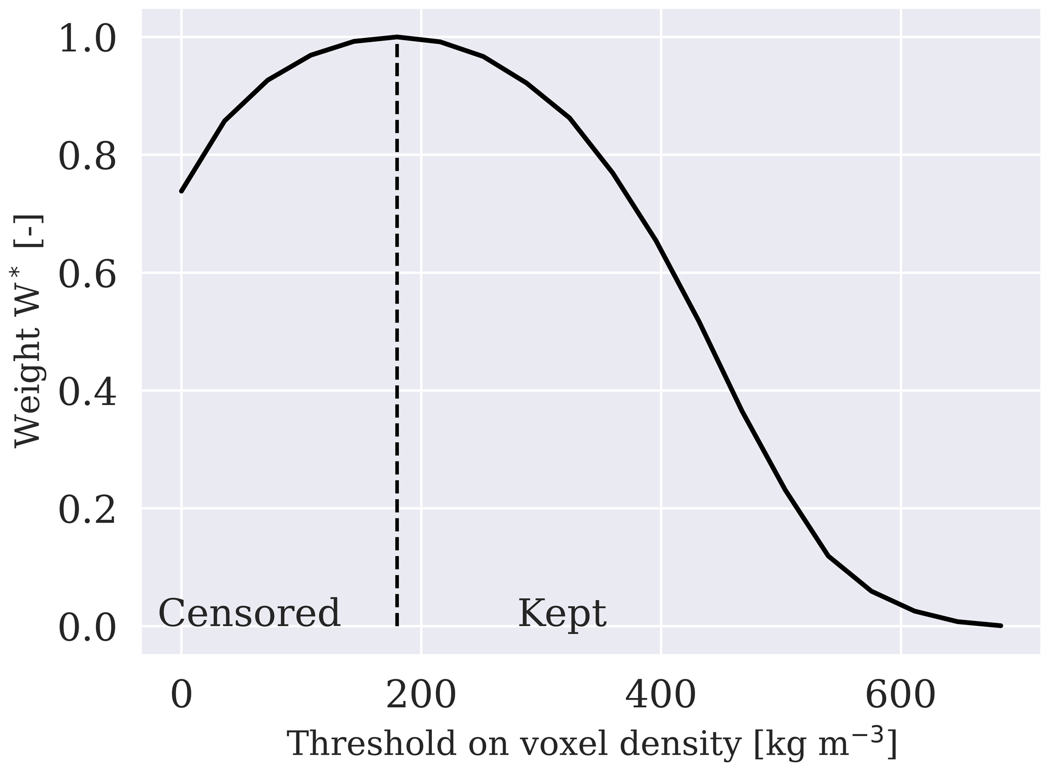
Figure A1Example, for a reconstructed snowflake, of the distribution of the weight W∗ as a function of the threshold on the voxel density content ρ. The weight is displayed here as normalized between 0 and 1. The threshold maximizing W∗ is considered optimal, and it is used to censor the data to calculate geometric descriptors. A maximum could always be obtained for all the reconstructed snowflakes.
The evolution of W∗ as a function of the threshold level has a behavior as illustrated in Fig. A1. We choose an optimal threshold corresponding to the location of maximum W∗ in order to balance the two errors. The final threshold is then applied to define the spatial extent assigned to the snowflake. In this work we used this approach to be able to evaluate the GAN output against the 3D-printed replicas, exclusively for quantities as Dmax or the convex hull volume. The total mass and the gyration radius are calculated on unfiltered data.
The code to generate simulated snowflakes is openly available: https://github.com/jleinonen/aggregation (Leinonen, 2021a). The 3D-GAN code is also available: https://github.com/jleinonen/masc3dgan (Leinonen, 2021b). The codes and data to support the evaluation of the performances of 3D-GAN, including the models and shapefiles of the replica snowflakes are published and available at Grazioli et al. (https://doi.org/10.5281/zenodo.4790962 2021). Raw or processed MASC data for any campaign mentioned in the paper, as well as a MATLAB code to preprocess the data according to the method by Praz et al. (2017) are available upon request to the authors.
JL and AB formulated the project and developed the methodology used in this study. JG performed the evaluation and the applications showed here. JL wrote the software code needed to implement the method. JG wrote the article with contributions from AB and JL.
Some authors are members of the editorial board of Atmospheric Measurement Techniques. The peer-review process was guided by an independent editor, and the authors have also no other competing interests to declare.
Publisher's note: Copernicus Publications remains neutral with regard to jurisdictional claims in published maps and institutional affiliations.
We thank Davide Ori and Adam Hicks for the constructive review of our paper. We would like to thank Julien Dorsaz and the Center of MicroNano Technology at EPFL for the useful exchanges and the 3D printing of snowflakes. We thank Alfonso Ferrone, EPFL-LTE, for the ideas, support and help to conduct the measurements with the replicas. We thank MeteoSwiss and the past and present members of EPFL-LTE for the MASC data of various field campaigns. We thank Boris Aguilar for sharing his implementation of the BL06 mass–size retrieval and several participants of the project ICEGENESIS (https://www.ice-genesis.eu/, last access: 15 October 2021) for the useful exchanges during the past months.
This research has been supported by the Swiss National Science Foundation (grant no. 200020_175700).
This paper was edited by Maximilian Maahn and reviewed by Adam Hicks and Davide Ori.
Alom, M. Z., Taha, T. M., Yakopcic, C., Westberg, S., Sidike, P., Nasrin, M. S., Hasan, M., Van Essen, B. C., Awwal, A. A. S., and Asari, V. K.: A State-of-the-Art Survey on Deep Learning Theory and Architectures, Electronics, 8, 292, https://doi.org/10.3390/electronics8030292, 2019. a
Arjovsky, M., Chintala, S., and Bottou, L.: Wasserstein GAN, arXiv [preprint], arXiv:1701.07875, 2017. a
Bagheri, A. and Jin, J.: Photopolymerization in 3D Printing, ACS Appl. Polym. Mat., 1, 593–611, https://doi.org/10.1021/acsapm.8b00165, 2019. a
Baker, B. and Lawson, R. P.: Improvement in determination of ice water content from two-dimensional particle imagery. Part I: Image-to-mass relationships, J. Appl. Meteorol. Clim., 45, 1282–1290, https://doi.org/10.1175/JAM2398.1, 2006. a, b
Chicco, D.: Siamese Neural Networks: An Overview, in: Artificial Neural Networks, edited by: Cartwright, H., Springer, New York, New York, USA, https://doi.org/10.1007/978-1-0716-0826-5_3, pp. 73–94, 2021. a
Dunnavan, E. L., Jiang, Z., Harrington, J. Y., Verlinde, J., Fitch, K., and Garrett, T. J.: The Shape and Density Evolution of Snow Aggregates, J. Atmos. Sci., 76, 3919–3940, https://doi.org/10.1175/JAS-D-19-0066.1, 2019. a, b, c
Fitch, K. E., Hang, C., Talaei, A., and Garrett, T. J.: Arctic observations and numerical simulations of surface wind effects on Multi-Angle Snowflake Camera measurements, Atmos. Meas. Tech., 14, 1127–1142, https://doi.org/10.5194/amt-14-1127-2021, 2021. a, b
Ford, B.: The Hidden Secrets of Snowflakes, Microscope, 62, 171–181, available at: http://www.mccroneinstitute.org/v/1021/The-Microscope-Volume-62-Fourth-Quarter-2014 (last access: 15 October 2021), 2014. a
Garrett, T. J. and Yuter, S. E.: Observed influence of riming, temperature, and turbulence on the fallspeed of solid precipitation, Geophys. Res. Lett., 41, 6515–6522, https://doi.org/10.1002/2014GL061016, 2014. a, b, c, d
Garrett, T. J., Fallgatter, C., Shkurko, K., and Howlett, D.: Fall speed measurement and high-resolution multi-angle photography of hydrometeors in free fall, Atmos. Meas. Tech., 5, 2625–2633, https://doi.org/10.5194/amt-5-2625-2012, 2012. a, b
Garrett, T. J., Yuter, S. E., Fallgatter, C., Shkurko, K., Rhodes, S. R., and Endries, J. L.: Orientations and aspect ratios of falling snow, Geophys. Res. Lett., 42, 4617–4622, 2015. a
Gavrilov, S., Kubo, M., Tran, V., Ngo, D., Nguyen, N., Nguyen, L., Lumbanraja, F., Phan, D., and Satou, K.: Feature Analysis and Classification of Particle Data from Two-Dimensional Video Disdrometer, Adv. Remote Sens., 4, 1–14, https://doi.org/10.4236/ars.2015.41001, 2015. a
Goodfellow, I., Pouget-Abadie, J., Mirza, M., Xu, B., Warde-Farley, D., Ozair, S., Courville, A., and Bengio, Y.: Generative Adversarial Nets, in: Advances in Neural Information Processing Systems 27, edited by: Ghahramani, Z., Welling, M., Cortes, C., Lawrence, N. D., and Weinberger, K. Q., Curran Associates, Inc., 2672–2680, available at: https://papers.nips.cc/paper/5423-generative-adversarial-nets.pdf (last access: 15 October 2021), 2014. a
Grazioli, J., Tuia, D., Monhart, S., Schneebeli, M., Raupach, T., and Berne, A.: Hydrometeor classification from two-dimensional video disdrometer data, Atmos. Meas. Tech., 7, 2869–2882, https://doi.org/10.5194/amt-7-2869-2014, 2014. a
Grazioli, J., Leinonen, J., and Berne, A.: Support data and codes for the evaluation experiment section of the paper: “Mass and geometry reconstruction of snowfall particles from multi angle snowflake camera (MASC) images”, Zenodo [data set and code], https://doi.org/10.5281/zenodo.4790962, 2021. a
Gulrajani, I., Ahmed, F., Arjovsky, M., Dumoulin, V., and Courville, A. C.: Improved Training of Wasserstein GANs, in: Advances in Neural Information Processing Systems 30, edited by: Guyon, I., Luxburg, U. V., Bengio, S., Wallach, H., Fergus, R., Vishwanathan, S., and Garnett, R., Curran Associates, Inc., 5767–5777, available at: https://papers.nips.cc/paper/7159-improved-training-of-wasserstein-gans.pdf (last access: 15 October 2021), 2017. a
Hicks, A. and Notaros, B. M.: Method for Classification of Snowflakes Based on Images by a Multi-Angle Snowflake Camera Using Convolutional Neural Networks, J. Atmos. Ocean. Tech., 36, 2267–2282, https://doi.org/10.1175/JTECH-D-19-0055.1, 2019. a
Jiang, Z., Oue, M., Verlinde, J., Clothiaux, E. E., Aydin, K., Botta, G., and Lu, Y.: What Can We Conclude about the Real Aspect Ratios of Ice Particle Aggregates from Two-Dimensional Images?, J. Appl. Meteorol. Clim., 56, 725–734, 2017. a
Jiang, Z., Verlinde, J., Clothiaux, E. E., Aydin, K., and Schmitt, C.: Shapes and Fall Orientations of Ice Particle Aggregates, J. Atmos. Sci., 76, 1903–1916, https://doi.org/10.1175/JAS-D-18-0251.1, 2019. a, b, c, d
Karrer, M., Seifert, A., Siewert, C., Ori, D., von Lerber, A., and Kneifel, S.: Ice Particle Properties Inferred From Aggregation Modelling, J. Adv. Model. Earth Sy., 12, e2020MS002066, https://doi.org/10.1029/2020MS002066, 2020. a, b, c, d, e
Kleinkort, C., Huang, G. J., Bringi, V. N., and Notaros, B. M.: Visual Hull Method for Realistic 3D Particle Shape Reconstruction Based on High-Resolution Photographs of Snowflakes in Free Fall from Multiple Views, J. Atmos. Ocean. Tech., 34, 679–702, https://doi.org/10.1175/JTECH-D-16-0099.1, 2017. a, b, c, d, e
Kruger, A. and Krajewski, W. F.: Two-dimensional video disdrometer: a description, J. Atmos. Ocean. Tech., 19, 602–617, 2002. a
Leinonen, J.: jleinonen/aggregation, Github [code], https://github.com/jleinonen/aggregation (last access: 15 October 2021), 2021a. a
Leinonen, J.: jleinonen/masc3dgan, Github [code], https://github.com/jleinonen/masc3dgan (last access: 15 October 2021), 2021b. a
Leinonen, J. and Berne, A.: Unsupervised classification of snowflake images using a generative adversarial network and K-medoids classification, Atmos. Meas. Tech., 13, 2949–2964, https://doi.org/10.5194/amt-13-2949-2020, 2020. a, b, c
Leinonen, J. and Moisseev, D.: What do triple-frequency radar signatures reveal about aggregate snowflakes?, J. Geophys. Res.-Atmos., 120, 2014JD022072, https://doi.org/10.1002/2014JD022072, 2015. a, b, c, d
Leinonen, J. and Szyrmer, W.: Radar signatures of snowflake riming: A modeling study, Earth and Space Science, 2, 2015EA000102, https://doi.org/10.1002/2015EA000102, 2015. a, b, c, d, e, f, g, h, i, j
Leinonen, J., Moisseev, D., and Nousiainen, T.: Linking snowflake microstructure to multi-frequency radar observations, J. Geophys. Res.-Atmos., 118, 3259–3270, https://doi.org/10.1002/jgrd.50163, 2013. a, b, c
Leinonen, J., Lebsock, M. D., Tanelli, S., Sy, O. O., Dolan, B., Chase, R. J., Finlon, J. A., von Lerber, A., and Moisseev, D.: Retrieval of snowflake microphysical properties from multifrequency radar observations, Atmos. Meas. Tech., 11, 5471–5488, https://doi.org/10.5194/amt-11-5471-2018, 2018. a
Leinonen, J., Nerini, D., and Berne, A.: Stochastic Super-Resolution for Downscaling Time-Evolving Atmospheric Fields With a Generative Adversarial Network, IEEE T. Geosci. Remote, 59, 7211–7223, https://doi.org/10.1109/tgrs.2020.3032790, 2021. a
Liu, C., Ikeda, K., Thompson, G., Rasmussen, R., and Dudhia, J.: High-Resolution Simulations of Wintertime Precipitation in the Colorado Headwaters Region: Sensitivity to Physics Parameterizations, Mon. Weather Rev., 139, 3533–3553, https://doi.org/10.1175/MWR-D-11-00009.1, 2011. a
Locatelli, J. D. and Hobbs, P. V.: Fall speeds and masses of solid precipitation particles, J. Geophys. Res., 79, 2185–2197, https://doi.org/10.1029/JC079i015p02185, 1974. a
Magono, C. and Lee, C. W.: Meteorological classification of natural snow crystals, J. Fac. Sci., Hokkaido Univ., Series VII, 2, 321–335, 1966. a
Mason, S. L., Chiu, C. J., Hogan, R. J., Moisseev, D., and Kneifel, S.: Retrievals of Riming and Snow Density From Vertically Pointing Doppler Radars, J. Geophys. Res.-Atmos., 123, 13807–13834, https://doi.org/10.1029/2018JD028603, 2018. a, b
Matrosov, S. Y., Clark, K. A., and Kingsmill, D. E.: A polarimetric radar approach to identify rain, melting-layer, and snow regions for applying corrections to vertical profiles of reflectivity, J. Appl. Meteorol. Clim., 46, 154–166, 2007. a, b
Morrison, H., van Lier-Walqui, M., Fridlind, A. M., Grabowski, W. W., Harrington, J. Y., Hoose, C., Korolev, A., Kumjian, M. R., Milbrandt, J. A., Pawlowska, H., Posselt, D. J., Prat, O. P., Reimel, K. J., Shima, S.-I., van Diedenhoven, B., and Xue, L.: Confronting the Challenge of Modeling Cloud and Precipitation Microphysics, J. Adv. Model. Earth Sy., 12, e2019MS001689, https://doi.org/10.1029/2019MS001689, 2020. a
Nešpor, V., Krajewski, W. F., and Kruger, A.: Wind-induced error of raindrop size distribution measurement using a two-dimensional video disdrometer, J. Atmos. Ocean. Tech., 17, 1483–1492, 2000. a
Newman, A. J., Kucera, P. A., and Bliven, L. F.: Presenting the Snowflake Video Imager (SVI), J. Atmos. Ocean. Tech., 26, 167–179, https://doi.org/10.1175/2008JTECHA1148.1, 2009. a
Praz, C., Roulet, Y.-A., and Berne, A.: Solid hydrometeor classification and riming degree estimation from pictures collected with a Multi-Angle Snowflake Camera, Atmos. Meas. Tech., 10, 1335–1357, https://doi.org/10.5194/amt-10-1335-2017, 2017. a, b, c, d, e, f, g, h, i, j, k, l, m, n, o, p, q, r
Pruppacher, H. R. and Klett, J. D.: Microphysics of clouds and precipitation, 2nd rev. and enl. edn., with an introduction to cloud chemistry and cloud electricity edn., Kluwer Academic Publishers, Dordrecht, 2000. a
Schaer, M., Praz, C., and Berne, A.: Identification of blowing snow particles in images from a Multi-Angle Snowflake Camera, The Cryosphere, 14, 367–384, https://doi.org/10.5194/tc-14-367-2020, 2020. a, b
Seifert, A., Leinonen, J., Siewert, C., and Kneifel, S.: The Geometry of Rimed Aggregate Snowflakes: A Modeling Study, J. Adv. Model. Earth Sy., 11, 712–731, https://doi.org/10.1029/2018MS001519, 2019. a
Takahashi, T.: Influence of Liquid Water Content and Temperature on the Form and Growth of Branched Planar Snow Crystals in a Cloud, J. Atmos. Sci., 71, 4127–4142, https://doi.org/10.1175/JAS-D-14-0043.1, 2014. a
Thompson, G., Field, P. R., Rasmussen, R. M., and Hall, W. D.: Explicit Forecasts of Winter Precipitation Using an Improved Bulk Microphysics Scheme. Part II: Implementation of a New Snow Parameterization, Mon. Weather Rev., 136, 5095–5115, https://doi.org/10.1175/2008MWR2387.1, 2008. a
Tridon, F., Battaglia, A., Chase, R. J., Turk, F. J., Leinonen, J., Kneifel, S., Mroz, K., Finlon, J., Bansemer, A., Tanelli, S., Heymsfield, A. J., and Nesbitt, S. W.: The Microphysics of Stratiform Precipitation During OLYMPEX: Compatibility Between Triple-Frequency Radar and Airborne In Situ Observations, J. Geophys. Res.-Atmos., 124, 8764–8792, https://doi.org/10.1029/2018JD029858, 2019. a
von Lerber, A., Moisseev, D., Bliven, L. F., Petersen, W., Harri, A.-M., and Chandrasekar, V.: Microphysical Properties of Snow and Their Link to Z(e)-S Relations during BAECC 2014, J. Appl. Meteorol. Clim., 56, 1561–1582, https://doi.org/10.1175/JAMC-D-16-0379.1, 2017. a, b, c, d, e, f
Weitzel, M., Mitra, S. K., Szakáll, M., Fugal, J. P., and Borrmann, S.: Application of holography and automated image processing for laboratory experiments on mass and fall speed of small cloud ice crystals, Atmos. Chem. Phys., 20, 14889–14901, https://doi.org/10.5194/acp-20-14889-2020, 2020. a
Yang, B., Wen, H., Wang, S., Clark, R., Markham, A., and Trigoni, N.: 3D Object Reconstruction from a Single Depth View with Adversarial Learning, in: 16th IEEE International Conference on Computer Vision (ICCV), Venice, ITALY, 22–29 October 2017, 679–688, https://doi.org/10.1109/ICCVW.2017.86, 2017. a
Zhou, Q.-Y., Park, J., and Koltun, V.: Open3D: A Modern Library for 3D Data Processing, arXiv: preprint, available at: https://arxiv.org/abs/1801.09847 (last access: 15 October 2021), 2018. a
See https://www.nanoscribe.com/en/products/photonic-professional-gt2, (last access: 15 October 2021).
Note that am is often given in cgs units in published research, while the mkgs convention is used in the tables of the present paper.
- Abstract
- Introduction
- The multi-angle snowflake camera (MASC)
- Methods
- Evaluation
- Examples of application
- Summary, conclusions and outlook
- Appendix A: Approximation of geometrical features
- Code and data availability
- Author contributions
- Competing interests
- Disclaimer
- Acknowledgements
- Financial support
- Review statement
- References