Retrieving microphysical properties of concurrent pristine ice and snow using polarimetric radar observations

Ice and mixed-phase clouds play a key role in our climate system because of their strong controls on global precipitation and radiation budget. Their microphysical properties have been characterized commonly by polarimetric radar measurements. However, there remains a lack of robust estimates of microphysical properties of concurrent pristine ice and aggregates because larger snow aggregates often dominate the radar signal and mask contributions of smaller pristine ice crystals. This paper presents a new method that separates the scattering signals of pristine ice embedded in snow aggregates in scanning polarimetric radar observations and retrieves their respective abundances and sizes for the first time. This method, dubbed ENCORE-ice, is built on an iterative stochastic ensemble retrieval framework. It provides the number concentration, ice water content, and effective mean diameter of pristine ice and snow aggregates with uncertainty estimates. Evaluations against synthetic observations show that the overall retrieval biases in the combined total microphysical properties are within 5 % and that the errors with respect to the truth are well within the retrieval uncertainty. The partitioning between pristine ice and snow aggregates also agrees well with the truth. Additional evaluations against in situ cloud probe measurements from a recent campaign for a stratiform cloud system are promising. Our median retrievals have a bias of 98 % in the total ice number concentration and 44 % in the total ice water content. This performance is generally better than the retrieval from empirical relationships. The ability to separate signals of different ice species and to provide their quantitative microphysical properties will open up many research opportunities, such as secondary ice production studies and model evaluations for ice microphysical processes.

1 Introduction

Ice-containing clouds play an important role in Earth's radiation budget and global precipitation (Baran et al., 2009; Field and Heymsfield, 2015; Mulmenstadt et al., 2015; Li et al., 2014). Their formation and evolution involve processes of ice nucleation, ice multiplication, aggregation, and riming, which are closely linked to atmospheric conditions and dynamics (DeMott et al., 2011; Field et al., 2017; Gultepe et al., 2017; Korolev et al., 2020). Such complex interactions make it challenging to complete our understanding of these ice microphysical processes and represent them well in models (Korolev et al., 2017; Morrison et al., 2020).

Polarimetric radar measurements contain information on ice properties and have been proven useful for studying ice microphysical processes (e.g. Kennedy and Rutledge, 2011; Grazioli et al., 2015; Moisseev et al., 2015). Many empirical relationships were developed to provide important bulk properties such as the ice water content (e.g. Ryzhkov et al., 1998; Lu et al., 2015), median volume diameter, and number concentration (e.g. Murphy et al., 2020), but they cannot inform the partitioning between ice species. The ability of the partitioning is of particular importance for studying the aggregation process because it provides information on the size and number concentration of pristine ice and aggregates.

However, separating signals of pristine ice from aggregates in polarimetric radar data is challenging because larger snow aggregates often dominate the radar reflectivity and mask contributions of smaller pristine ice crystals (Hogan et al., 2002; Keat and Westbrook, 2017). As a result, information from horizontal reflectivity (Z_H) alone is insufficient to characterize mixtures of ice hydrometeors (Oue et al., 2018), and it is necessary to incorporate other radar observables in retrieval methods. By exploiting distinct fall behaviours between pristine ice and aggregates, Spek et al. (2008) used Z_H, differential reflectivity (Z_DR), and the Doppler spectrum to retrieve particle size distribution (PSD) parameters of pristine ice and snow aggregates. Without the use of the Doppler spectrum, Schrom et al. (2015) used Z_H, Z_DR, and specific differential phase shift (K_DP) to estimate the PSD of pristine ice in the dendritic growth zone of Colorado winter storms. K_DP is a great addition in their approach since it is mainly determined by ice number concentration. Unfortunately, these three radar observables remain insufficient, and their partitioning between pristine ice and aggregates was weakly constrained. To improve the partitioning, Keat and Westbrook (2017) showed that the relative radar signal contributions of pristine ice embedded in snow aggregate populations can be quantified using Z_H, Z_DR, and the co-polar correlation coefficient (ρ_hv), but they have not attempted to use their partitioning to provide quantitative retrievals of pristine-ice number concentration, water content, and particle size.

The objective of the paper is to present an ensemble cloud retrieval method (dubbed ENCORE-ice) for simultaneously retrieving the number concentrations, sizes, and ice water contents of concurrent pristine ice and snow aggregates from measurements of Z_H, Z_DR, K_DP, and ρ_hv. This framework provides full error statistics and characterizes sub-species from radar signals, which is an advance on the existing methods. The polarimetric radar observations and the retrieval method are detailed in Sect. 2. The ancillary datasets for evaluations are introduced in Sect. 3. Section 4 presents evaluation results using synthetic datasets and actual observations from Chilbolton, United Kingdom, in 2018. Finally, Sect. 5 summarizes the key findings and discusses potential applications.

2 Radar observations and ENCORE-ice

2.1 Polarimetric radar data

Our retrieval method uses four polarimetric observables. The first observable is the horizontal reflectivity Z_H, which provides information on particle size and concentration, but its dependence on size is much stronger. As such, Z_H is dominated by contributions from snow aggregates because their sizes, and thus their backscatter cross-sections, are typically much larger than those of pristine ice crystals. The second observable is the differential reflectivity Z_DR, which provides information on particle shape and orientation. A Z_DR of 0 dB indicates spherical particles because of equal backscattered power in each polarization. Snow aggregates yield low Z_DR values (about 0–0.6 dB; see Hogan et al., 2012) as a result of their sparse and irregular morphology, with the component crystals oriented at a wide range of angles. In contrast, pristine ice particles can yield Z_DR values of several decibels because of their aspect ratios and preferential horizontal orientation when falling. Heterogenous regions with concurrent pristine ice and snow aggregates are therefore associated with higher Z_DR values than if only snow aggregates were present. The third observable is the co-polar correlation coefficient ρ_hv, the correlation coefficient between horizontally and vertically backscattered power, which provides information on the diversity of particle shape in a radar sample volume (Kumjian, 2013; Keat et al., 2016). ρ_hv is unity in homogenous regions but tends towards lower values (e.g. ∼ 0.97) in the presence of heterogenous hydrometeor types. Finally, the fourth observable is the specific differential phase shift K_DP, which provides information on particle number concentration, shape, and orientation.

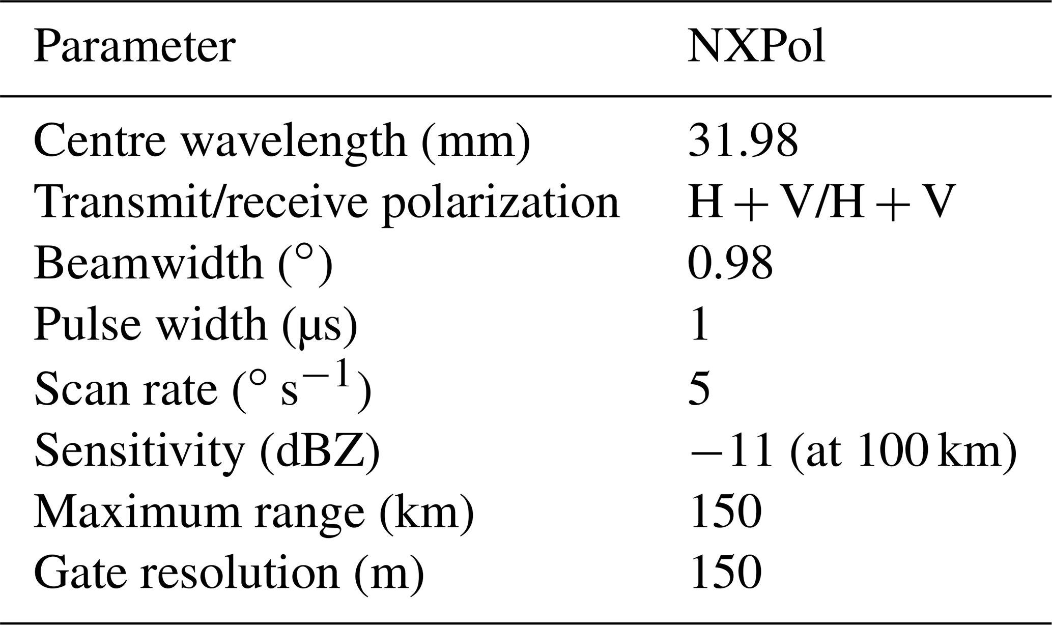
Our case study is based on polarimetric radar data (Bennett, 2020) from the Parameterizing Ice Clouds using Airborne obServationS and triple-frequency dOppler radar data (PICASSO) field campaign in Chilbolton, UK, in 2018–2019. During the campaign, the National Centre for Atmospheric Science mobile X-band dual-polarization Doppler weather radar (NXPol; Neely et al., 2018) operated with a 0.98^∘ beam width, 150 m range resolution, and maximum range of 150 km. The radar performed two back-to-back, fixed-azimuth range–height indicator (RHI) scans every 7 min, and each scan was completed in 18 s. Throughout 13 February 2018, RHI scans were performed along the 243^∘ radial and intercepted by the NCAS-managed Facility for Airborne Atmospheric Measurements (FAAM) aircraft on several occasions, providing a unique opportunity for evaluation. Key characteristics of NXPol are summarized in Table 1.

Table 1 Characteristics of the NXPol polarimetric radar. Further specifications and details can be found in Neely et al. (2018).

2.2 ENCORE-ice

ENCORE is an ensemble-based retrieval method that has previously been used to retrieve three-dimensional cloud microphysical properties (Fielding et al., 2014) and one-dimensional cloud and drizzle properties (Fielding et al., 2015), but several key components are modified here for ice retrieval.

2.2.1 Particle size distribution

We approximate the PSD of pristine ice and aggregates by normalized gamma distributions, given as (Testud et al., 2001)

$$\begin{array}{}\text{(1)}& n\left(D\right)=N_{\mathrm{0}}{f}_{\mathit{\mu }}\left(D;D_{\mathrm{0}}\right),\end{array}$$

where N₀ is the normalized number concentration and n(D)dD is the number of particles in the range of the maximum particle dimensions ($D,D+\mathrm{d}D$). The choice of the size descriptor in Eq. (1) is because in situ cloud probe data and the ice scattering database are both given based on the maximum particle dimension. The function f_μ is defined as

$$\begin{array}{}\text{(2)}& \begin{array}{rl}{f}_{\mathit{\mu }}\left(D;D_{\mathrm{0}}\right)& ={\displaystyle \frac{\mathrm{6}}{{\mathrm{3.67}}^{\mathrm{4}}}}\cdot {\displaystyle \frac{{\left(\mathrm{3.67}+\mathit{\mu }\right)}^{\mathrm{4}+\mathit{\mu }}}{\mathrm{\Gamma }\left(\mathrm{4}+\mathit{\mu }\right)}}{\left({\displaystyle \frac{D}{D_{\mathrm{0}}}}\right)}^{\mathit{\mu }}\\ & \cdot \exp \left[-\left(\mathrm{3.67}+\mathit{\mu }\right){\displaystyle \frac{D}{D_{\mathrm{0}}}}\right],\end{array}\end{array}$$

where μ is the shape parameter of the PSD and D₀ is the diameter used for normalizing D. Following Mason et al. (2018), we assume a constant shape parameter of μ=2. Several studies have shown that the retrieved ice water content is relatively insensitive to the choice of shape parameter (e.g. Delanoë et al., 2005; Spek et al., 2008); we also found that our number concentration retrieval is not sensitive to μ.

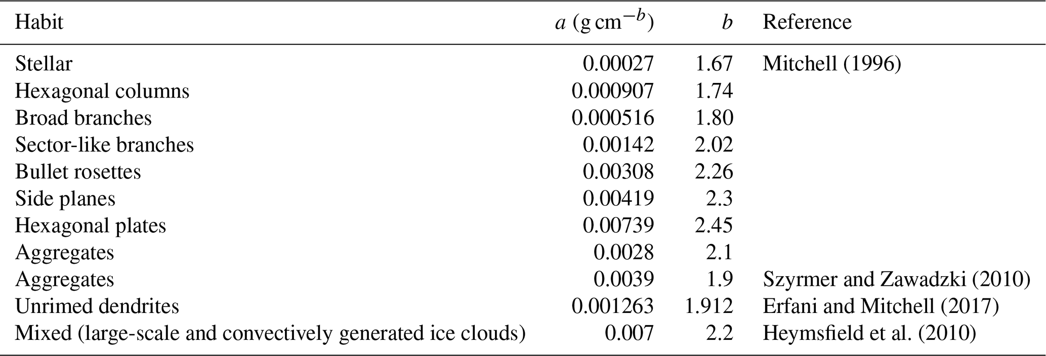
Table 2 Examples of mass–size relationships (taken from Mason et al., 2018).

From the PSD, the total ice number concentration (N_I) and the total ice water content (q_I) can be computed by

$$\begin{array}{}\text{(3)}& \begin{array}{rl}{N}_{\mathrm{I}}& =\underset{\mathrm{0}}{\overset{\mathrm{\infty }}{\int }}n\left(D\right)\mathrm{d}D=\underset{\mathrm{0}}{\overset{\mathrm{\infty }}{\int }}\left[n_{\mathrm{P}}\left(D\right)+n_{\mathrm{A}}\left(D\right)\right]\mathrm{d}D\\ & =\underset{\mathrm{0}}{\overset{\mathrm{\infty }}{\int }}{N}_{\mathrm{0},\mathrm{P}}{f}_{\mathit{\mu }}\left(D;D_{\mathrm{0},\mathrm{P}}\right)\mathrm{d}D+\underset{\mathrm{0}}{\overset{\mathrm{\infty }}{\int }}{N}_{\mathrm{0},\mathrm{A}}{f}_{\mathit{\mu }}\left(D;D_{\mathrm{0},\mathrm{A}}\right)\mathrm{d}D\\ & =N_{\mathrm{P}}+N_{\mathrm{A}}\end{array}\end{array}$$

and

$$\begin{array}{}\text{(4)}& \begin{array}{rl}{q}_{\mathrm{I}}& =\underset{\mathrm{0}}{\overset{\mathrm{\infty }}{\int }}m\left(D\right)n\left(D\right)\mathrm{d}D\\ & =\underset{\mathrm{0}}{\overset{\mathrm{\infty }}{\int }}{m}_{\mathrm{P}}\left(D\right)n_{\mathrm{P}}\left(D\right)\mathrm{d}D+\underset{\mathrm{0}}{\overset{\mathrm{\infty }}{\int }}{m}_{\mathrm{A}}\left(D\right)n_{\mathrm{A}}\left(D\right)\mathrm{d}D\\ & =q_{\mathrm{P}}+q_{\mathrm{A}},\end{array}\end{array}$$

respectively, where n(D) is the combined PSD from n_P(D)+n_A(D) and the subscripts P and A denote contributions from pristine ice and snow aggregates, respectively. m(D) is the mass at a given maximum particle dimension D. The mass–size relationship can be formulated as

$$\begin{array}{}\text{(5)}& m\left(D\right)=a{D}^b,\end{array}$$

where a and b are the pre-factor and exponent, respectively. These coefficients depend on ice habit and have been estimated from past aircraft in situ and surface observations as shown in Table 2. From the PSD, we define and calculate the effective mean diameters (D_eff) as

$$\begin{array}{}\text{(6)}& D_{\mathrm{eff}}={\displaystyle \frac{{\int }_{\mathrm{0}}^{\mathrm{\infty }}n\left(D\right)D^{\mathrm{4}}\mathrm{d}D}{{\int }_{\mathrm{0}}^{\mathrm{\infty }}n\left(D\right)D^{\mathrm{3}}\mathrm{d}D}},\end{array}$$

which is the ratio of the fourth to the third moment of the PSD. To compare our retrieval with the empirical estimates (as discussed in Sect. 3), we also calculate an effective mean diameter using the equivalent melted diameter (D_mlt) as the size descriptor, defined as

$$\begin{array}{}\text{(7)}& D_{\mathrm{eff},\mathrm{mlt}}={\displaystyle \frac{{\int }_{\mathrm{0}}^{\mathrm{\infty }}n\left(D_{\mathrm{mlt}}\right)D_{\mathrm{mlt}}^{\mathrm{4}}\mathrm{d}{D}_{\mathrm{mlt}}}{{\int }_{\mathrm{0}}^{\mathrm{\infty }}n\left(D_{\mathrm{mlt}}\right)D_{\mathrm{mlt}}^{\mathrm{3}}\mathrm{d}{D}_{\mathrm{mlt}}}},\end{array}$$

where

$$\begin{array}{}\text{(8)}& D_{\mathrm{mlt}}={\left[{\displaystyle \frac{\mathrm{6}m\left(D\right)}{\mathit{\pi }{\mathit{\rho }}_{\mathrm{w}}}}\right]}^{\frac{\mathrm{1}}{\mathrm{3}}}={\left[{\displaystyle \frac{\mathrm{6}a{D}^b}{\mathit{\pi }{\mathit{\rho }}_{\mathrm{w}}}}\right]}^{\frac{\mathrm{1}}{\mathrm{3}}}\end{array}$$

and ρ_w is water density.

2.2.2 The basis of ENCORE-ice

The state vector (x, i.e. variables to be retrieved) for each ensemble member is defined as

$$\begin{array}{}\text{(9)}& \begin{array}{rl}\mathit{x}=& \left({\log }_{\mathrm{10}}{N}_{\mathrm{0},\mathrm{P}}^{\left(i=\mathrm{1}\mathrm{\dots }G\right)},{\log }_{\mathrm{10}}{D}_{\mathrm{0},\mathrm{P}}^{\left(i=\mathrm{1}\mathrm{\dots }G\right)},{\log }_{\mathrm{10}}{N}_{\mathrm{0},\mathrm{A}}^{\left(i=\mathrm{1}\mathrm{\dots }G\right)},\right.\\ & {\left.{\log }_{\mathrm{10}}{D}_{\mathrm{0},\mathrm{A}}^{\left(i=\mathrm{1}\mathrm{\dots }G\right)}\right)}^T,\end{array}\end{array}$$

where the superscript i represents the index of the range gate and the total number of gates to be retrieved is G. Let us use Q members to form an ensemble; i.e.

$$\begin{array}{}\text{(10)}& \left\{{\mathit{x}}_{\mathrm{1}},\mathrm{\dots },{\mathit{x}}_Q\right\}\end{array}$$

such that the mean $\stackrel{\mathrm{‾}}{\mathit{x}}$ represents the best estimate of the state vector and the spread of the ensemble members around the mean represents the uncertainty in the best estimate.

Using the iterative stochastic ensemble Kalman filter approach (Evensen et al., 2019), each ensemble member is updated based on

$$\begin{array}{}\text{(11)}& {\mathit{x}}_k^{\mathrm{a}}={\mathit{x}}_k^{\mathrm{f}}+{\mathbf{E}}^{\mathrm{f}}{\mathit{w}}_k,\end{array}$$

in which ${\mathit{x}}_k^{\mathrm{f}}$ and ${\mathit{x}}_k^{\mathrm{a}}$ are the prior and posterior ensemble member k, respectively;

$$\begin{array}{}\text{(12)}& {\mathbf{E}}^{\mathrm{f}}=\left[{\mathit{x}}_{\mathrm{1}}^{\mathrm{f}}-{\stackrel{\mathrm{‾}}{\mathit{x}}}^{\mathrm{f}},\mathrm{\dots },{\mathit{x}}_Q^{\mathrm{f}}-{\stackrel{\mathrm{‾}}{\mathit{x}}}^{\mathrm{f}}\right]\end{array}$$

is the initial ensemble matrix with the prior mean (${\stackrel{\mathrm{‾}}{\mathit{x}}}^{\mathrm{f}}$) subtracted; and w_k comprises weight vectors that are calculated from iteratively minimizing the following cost function:

$$\begin{array}{}\text{(13)}& \begin{array}{rl}J\left({\mathit{w}}_k\right)& ={\displaystyle \frac{\mathrm{1}}{\mathrm{2}}}{\mathit{w}}_k^T{\mathit{w}}_k+{\displaystyle \frac{\mathrm{1}}{\mathrm{2}}}{\left(\mathit{y}-h\left({\mathit{x}}_k^{\mathrm{f}}+{\mathbf{E}}^{\mathrm{f}}{\mathit{w}}_k\right)-{\mathit{\epsilon }}_k\right)}^T\\ & \cdot {\mathbf{R}}^{-\mathrm{1}}\left(\mathit{y}-h\left({\mathit{x}}_k^{\mathrm{f}}+{\mathbf{E}}^{\mathrm{f}}{\mathit{w}}_k\right)-{\mathit{\epsilon }}_k\right).\end{array}\end{array}$$

In Eq. (13), the observation vector y is defined as gate-by-gate radar observables:

$$\begin{array}{}\text{(14)}& \begin{array}{rl}\mathit{y}=& \left(Z_{\mathrm{H}}^{(i=\mathrm{1},\mathrm{\dots },G)},Z_{\mathrm{DR}}^{(i=\mathrm{1},\mathrm{\dots },G)},-\ln K_{\mathrm{DP}}^{\left(i=\mathrm{1},\mathrm{\dots },G\right)},\right.\\ & {\left.-\ln {\mathit{\rho }}_{\mathrm{hv}}^{\left(i=\mathrm{1},\mathrm{\dots },G\right)}\right)}^T,\end{array}\end{array}$$

where Z_H and Z_DR are in decibels. Radar observations at one range gate will influence the estimation of the state vector at another gate if these two gates are within the pre-defined radius, which will be explained in more detail in Sect. 2.3. h(x) represents the forward model for simulating polarimetric radar observables from the state vector x, and ε_k is a random perturbation vector drawn from the observation error distribution, which is estimated to be Gaussian with a mean of zero and covariance matrix R (Evensen et al., 2019, with modification from Van Leeuwen, 2020). The covariance matrix R is diagonal with standard deviations given in Table 3.

Table 3 Estimated observational errors for X-band observables based on standard and benchmark procedures, adapted from Bringi and Chandrasekar (2001, pp. 359–376) and Wang and Chandrasekar (2009).

^a Estimated by the uncertainty of 0.05^∘ km⁻¹ for a typical value of K_DP=0.5^∘ km⁻¹. ^b Estimated by the uncertainty of 0.01 for ρ_hv=0.95.

As detailed later in Sect. 2.3, the prior is assumed Gaussian, and there is no prior correlation between variables N_0,P, D_0,P, N_0,A, and D_0,A. But there is correlation in the vertical (i.e. between gates) for each variable in our setup. We have also used a prior with large uncertainty, approximately 1–2 orders of magnitude in the state variables, such that the influence of the prior is minimal. In contrast to the prior, no Gaussian assumption is made in the posterior ensemble members, although the retrieval statistics are largely focused on their means and standard deviations.

2.2.3 Simulating radar observables for h(x)

To model polarimetric radar observables from the assumed PSD, knowledge of the single-scattering properties of ice particles is required. Many scattering databases of realistically shaped ice particles at radar wavelengths are available, and we used Lu et al. (2016) because of the following considerations. Several existing scattering databases assume a total random orientation of the scatterers, e.g. Liu (2008), Hong et al. (2009), Kuo et al. (2016), and Eriksson et al. (2018). Such assumption cannot explain polarimetric radar signals which are produced by non-spherical scatterers with preferred orientations with respect to the zenith direction. The database of Brath et al. (2020) assumes scatterers possess arbitrary fixed orientations relative to the zenith direction but includes only hexagonal plates and aggregates consisting of hexagonal plates. We found that the database described in Lu et al. (2016) fits our needs in the current polarimetric radar study since it contains all necessary polarimetric scattering data in many fixed orientations of a large variety of ice crystal species, including plates, columns, dendrites, and aggregates. The single-scattering properties for each species are available for a range of crystal maximum dimensions, thickness ratios, and types. The pristine habits generally begin at ∼ 0.1 mm and do not exceed 6 mm, whereas the aggregates begin at ∼ 0.4 mm and extend to approximately 18–45 mm. Multiple morphological realizations per maximum dimension are available for dendrites and aggregates to account for their complexities. Note that for a given size, natural aggregates may have substantially different properties compared to the realizations available in the database.

The scattering calculations were conducted using the generalized multi-particle Mie method (GMM; Xu, 1995) and the discrete dipole approximation (DDA; Yurkin and Hoekstra, 2011). We used properties calculated from GMM because DDA calculations are not available for aggregates. Specifically, we use the amplitude scattering matrix elements in the forward and backward direction for horizontally and vertically polarized radiation, denoted as $S_{\mathrm{hh}}^{\mathrm{f},\mathrm{b}}$ and $S_{\mathrm{vv}}^{\mathrm{f},\mathrm{b}}$, where the superscript and subscript represent the scattering direction (i.e. forward or background) and the polarization status (horizontally or vertically), respectively. From the assumed PSD and the amplitude scattering matrix elements, radar observables for a single sample volume containing multiple ice particle habits can be derived as shown in Appendix A.

2.3 Practical considerations

There are several practical considerations for ENCORE-ice implementation. The first consideration is ice habit. The scattering database provides three habits (plates, dendrites, and columns) for pristine ice. Since the temperature found in PICASSO mostly ranged between −5 and −25 ^∘C, all three types of pristine ice can be the preferred habit (see examples in Fig. 1). Currently, we do not predetermine the ice habit. Instead, we ran our retrieval algorithm for all three habits independently and then selected the most appropriate one based on the agreement in the measured and forward-simulated radar observables.

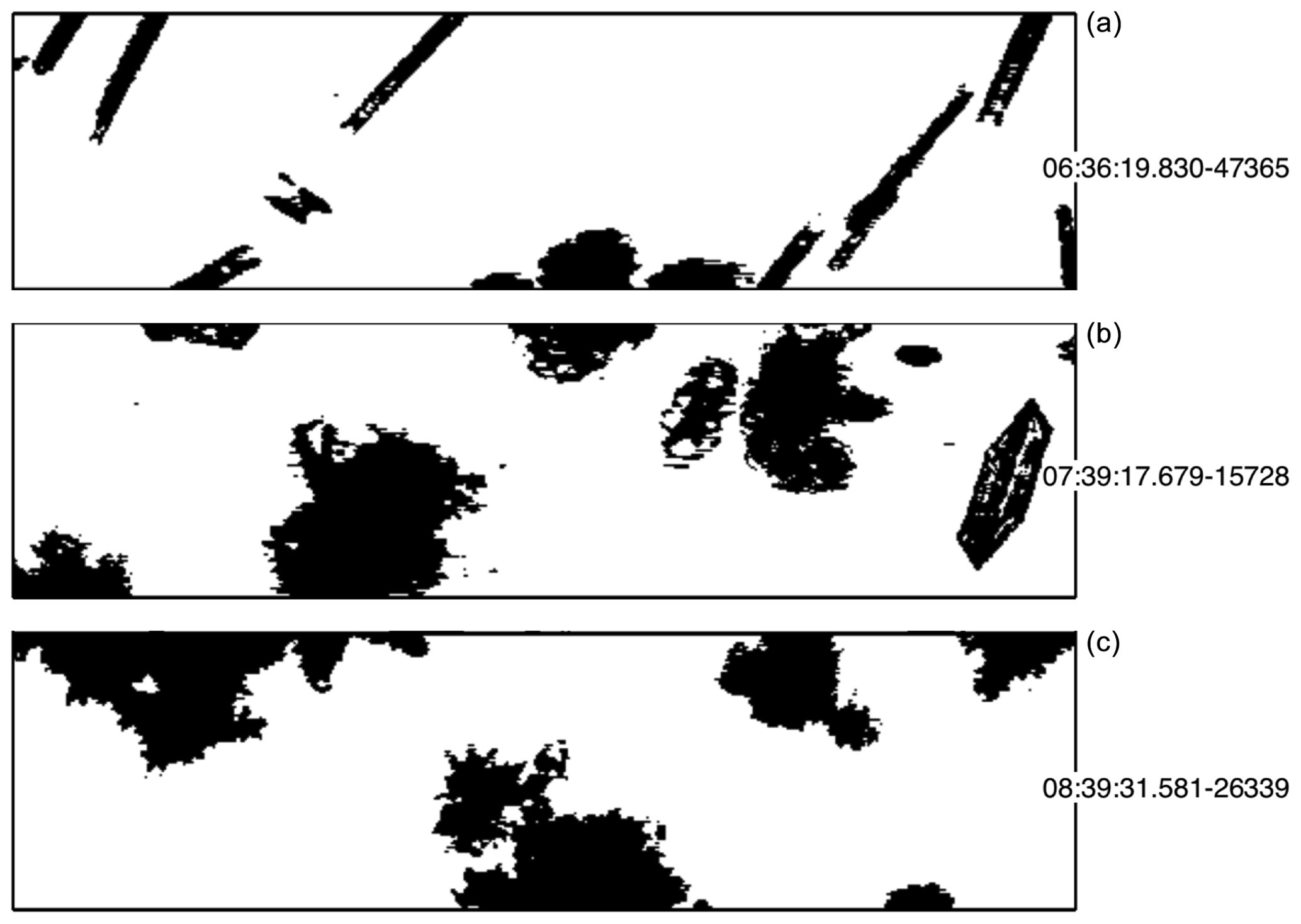
Figure 1 Examples of particle images from the Stratton Park Engineering Company Two-Dimension Stereo (2D-S) probe, showing the presence of (a) column, (b) plate, and (c) aggregates of dendrites on 13 February 2018. Each image frame is 1.28 mm high, taken from one of the probe channels only since the other channel was not working properly on this day.

Similarly, the scattering database provides five types of aggregates: two of them were constructed using ice columns (LD-N1e and HD-N1e) and three of them using stellar ice crystals (LD-P1d, LDt-P1d, and HD-P1d). Each aggregate in the database (Lu et al., 2016) was generated by first specifying a reference spheroid with a given horizontal maximum dimension and an aspect ratio of 0.6, defined as the ratio of the lengths of the polar axes to the equatorial axes. Then, small monomers were added to the reference spheroid one at a time; any parts of the monomer that were outside the reference spheroid were removed. This procedure was repeated until the mass of the aggregate reached the desired total mass. As a result, the aspect ratio of the aggregate generated in the database was not necessarily the same as the reference spheroid (0.6).

Figure 2 shows the average aspect ratios for aggregate types available in the database, which were calculated by averaging ratios of the maximum vertical dimension to the maximum horizontal dimension for all realizations within one size bin. Compared to Garrett et al. (2015) and Jiang et al. (2017), who reported an aspect ratio range between 0.3 to 0.6 from observations of falling aggregates at the surface, we found that LDt-P1d and HD-P1d exhibit a similar aspect ratio range. In the mass–size relationship for LDt-P1d we used a=0.000482 and b=1.97 in units of centimetres, grams, and seconds (cgs) as in Table 2, based on aggregates composed of ordinary dendritic crystal (Kajikawa, 1989; Botta et al., 2011), whereas for HD-P1d we used a=0.00145 and b=1.80 in units of cgs, based on aggregates of thin plate (Mitchell and Heymsfield, 2005; Botta et al., 2011). The mass–size relationship of HD-P1d is very close to unrimed aggregates (Erfani and Mitchell, 2017) and more aligned to values in the recent literature listed in Table 2. Hence, we select HD-P1d as the prescribed choice for aggregates.

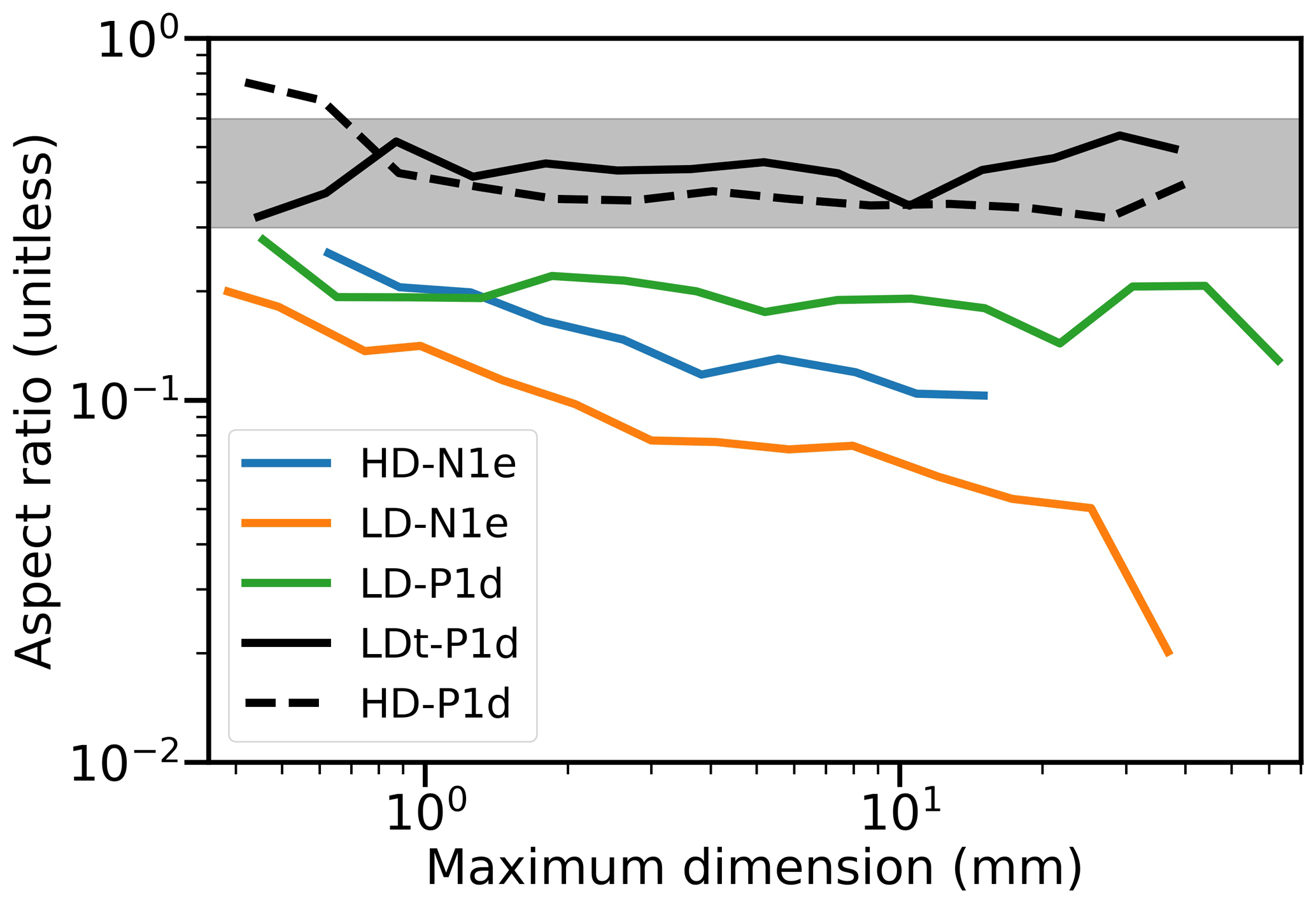
Figure 2 Aspect ratios of various aggregate types available in the scattering database as a function of their maximum dimensions. The aspect ratio is defined as the ratio of the sizes of the minor axes to the major axes. The grey shading between 0.3 and 0.6 represents the typical range of snow aggregate aspect ratios observed in nature (Garrett et al., 2015; Jiang et al., 2017).

The second consideration is the prior used to generate the first guess for ensemble members. Using over 70 h of in situ aircraft observations from a wide range of field campaigns spanning diverse cloud and temperature regimes, Delanoë et al. (2014) characterized the PSDs of ice particles by the normalized gamma distribution. They found that N₀ ranged between 1 and 10 000 L⁻¹ mm⁻¹ with a mean of 100 L⁻¹ mm⁻¹, and the median volume diameter (MVD) ranged between 0.2–0.8 mm with a mean of 0.5 mm for the temperature zone of −10 to −20 ^∘C. Additionally, Tiira et al. (2016) analysed surface measurements of ice particle number concentration from the Precipitation Imaging Package during the Biogenic Aerosols – Effects on Clouds and Climate field campaign. They found that N₀ ranged mainly from 1 to 100 L⁻¹ mm⁻¹ and MVD ranged from 0.5 to 5 mm. As these were surface based, the measured PSDs from Tiira et al. (2016) are more representative of the characteristics of snow aggregates. Note that these values were derived using the equivalent melted diameter as the size descriptor, not the maximum particle dimension. Hence, these values are used only to point out a possible range and serve as a starting point for us to construct the prior.

Table 4 The prior and uncertainty used in ENCORE-ice. The means at the lowest radar gate are given in the physical state space, and the rest are in the transformed state space (i.e. log ₁₀). Retrieval is performed using two different sets of the prior; the second set uses values in the parentheses, and the rest remain unchanged. All radar gates above the lowest gates are perturbed by an AR1 red noise process with a vertical correlation of 0.999 and a standard deviation that is half of the standard deviation at the lowest gates.

Based on these observational ranges mentioned above, our prior is designed as follows. We started with the lowest radar gate, randomly assigning (N_0,P, D_0,P, N_0,A, D_0,A) from normal distributions with the means and standard deviations listed in Table 4. Next, we applied a slope for each ray to provide initial guesses for other radar gates. The slope was randomly selected from a normal distribution described in Table 4. Because the prevalence of active ice nuclei is a function of temperature and thus a function of height as well (DeMott et al., 2010), N_0,P likely increases with height, and thus the slopes in the prior are assumed to have a positive mean. In contrast, the dependence of D_0,P, N_0,A, and D_0,A on height is less clear (e.g. Field et al., 2005). For practical reasons, the slopes applied for D_0,P, N_0,A, and D_0,A are assumed to have a slightly negative mean. The slightly negative slope avoids unrealistic priors for radar gates at higher altitudes since we used the logarithm form in the state vector. Finally, red (AR1) noise was added over the vertical with a correlation coefficient of 0.999 and a zero-mean random perturbation with a standard deviation that is half that of the lowest radar gate. Note that without this noise term each ensemble member would be a straight line in the vertical for each variable with a different slope. Since the fundamental idea behind ensemble retrievals is that the true atmospheric profile is drawn from the same distribution as the prior ensemble members and we know the true atmospheric profile is not a straight line, we add random noise with non-zero vertical correlation to each ensemble member profile to make each of them more realistic.

Compared to values reported in Delanoë et al. (2014) and Tiira et al. (2016), we have chosen lower means for N_0,P and N_0,A to start with. This is because the state vector space is the logarithm of N₀. Positive slopes make the changes in N₀ much more dramatic in the vertical than those with negative slopes. As a result, large starting values of N_0,P and N_0,A will lead to unrealistically high concentrations at higher altitudes in the prior. In contrast, we choose larger means for D_0,P and D_0,A because of the assumed negative slopes in both D_0,P and D_0,A. In general, the range in our prior is large, approximately 1–2 orders of magnitude across all ensemble members over all the vertical profiles. For such a widely spread prior the solution will be dominated by the observations.

The third consideration is the number of the ensemble members used in ENCORE-ice. Ideally, a large ensemble size is needed to ensure that the sampled prior, as well as the solution, is representative. However, a large ensemble size is computationally expensive. Therefore, we applied a localization scheme to reduce the required number of ensemble members so that we shorten the computational time while achieving the same mean retrieval and associated uncertainty. The localization scheme operates on each gate and takes only observations close to that gate into account to find the solution. This is implemented by multiplying the observation error variance of each observation with an exponential function of the distance between that observation and the gate that is being updated, such that observations far from the gate have less influence. The influence radii vary linearly with height, with one gate at the lower level and about five gates at the upper level. Using our synthetic datasets, we have found that 50 ensemble members with the localization scheme are able to produce similar mean retrievals and associated uncertainty to a non-localized ensemble of size 500. The number of iterations is set to 20, although the solutions often converge at the 10th iteration.

Finally, all radar data underwent the following quality checks and corrections before being used for retrieval:

• Z_H and Z_DR were corrected for attenuation due to liquid water, using the method described in Bringi and Chandrasekar (2001, pp. 490–512). The attenuation due to ice at the X-band is negligible and thus ignored here (Vivekanandan et al., 1999).

• Systematic biases in Z_DR were identified using zenith-pointing Z_DR observations. As hydrometeors produce a Z_DR of 0 dB when viewed at the zenith angle due to their spherical symmetry (e.g. for raindrops) or lack of preferential azimuthal orientation (e.g. for ice particles), any residual Z_DR can be treated as bias and removed (Seliga et al., 1981). We have found the Z_DR correction factors to be 0.2 dB for the PICASSO cases.

• K_DP was calculated using the method of Wang and Chandrasekar (2009).

• Once all corrections are applied, measurement noises were removed using a cubic spline approach (Craven and Wahba, 1979).

Additionally, to ensure that gates are associated with sufficient information for our method, we exclude gates that exhibit one or more of the following conditions:

• gates within 500 m of the 0 ^∘C level, avoiding contamination from liquid hydrometeors in the radar sample volume because our state vector is not designed for that;

• gates where ρ_hv exceeds 1.0 because these values are unphysical;

• gates with a signal-to-noise ratio (SNR) of less than 20 dB because of a lack of detectable hydrometeors, a threshold chosen because the precipitating region and its surrounding area typically have SNR values larger than 30–40 dB;

• radar rays with elevation angles greater than 50^∘ because Z_DR tends towards 0 dB at higher elevation angles and polarimetric information becomes ambiguous;

• gates with Z_DR below 0.25 dB, regardless of their elevation angles, because the relative contributions of pristine ice and aggregates become ambiguous at lower values, as indicated in Keat and Westbrook (2017);

• gates with K_DP below 0.1^∘ km⁻¹ to ensure a sufficient number concentration of pristine ice.

Note that negative K_DP values indicate the presence of conical graupel (Aydin and Seliga, 1984) or the vertical reorientation of pristine ice crystals in the presence of thunderstorm electric fields (Hubbert et al., 2014). Since our state vector includes only aggregates and horizontally oriented pristine ice, excluding gates with low K_DP values is necessary.

3 Independent observations and retrievals for evaluations

3.1 In situ aircraft measurements from PICASSO

During PICASSO, the FAAM aircraft performed multiple transects from Chilbolton to Dorset (50.82^∘ N, 2.56^∘ W) at varied altitudes. Figure 3 depicts the flight path for 13 February 2018, which was a typical pattern during the campaign.

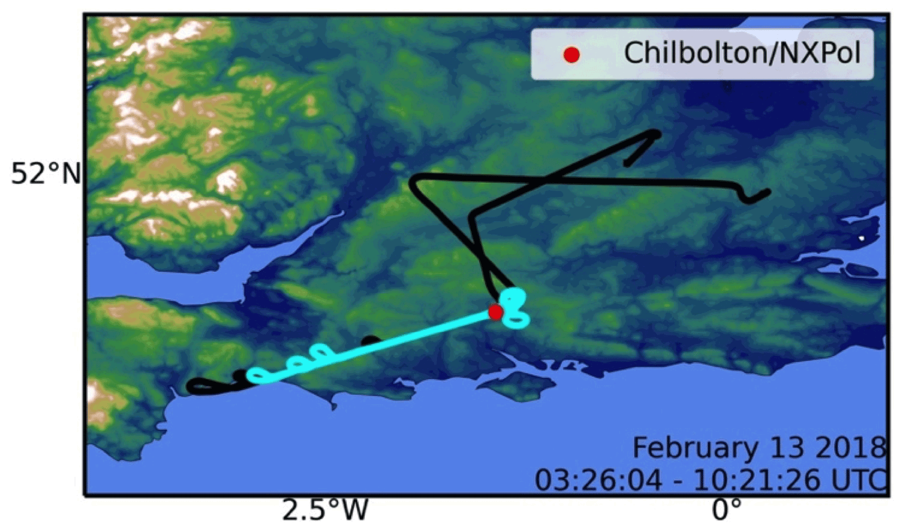
Figure 3 Flight paths on 13 February 2018 between 03:26 and 10:21 UTC. The red dot denotes the location of NXPol in Chilbolton, UK, while the path in cyan denotes the path during 06:00–09:00 UTC in which retrievals are evaluated in Sect. 4.2.

To evaluate our cloud retrieval, we use in situ measurements of liquid water content and total water content (i.e. the sum of ice and liquid water contents) from a Nevzorov probe and PSD measurements from a high-volume precipitation spectrometer (HVPS; SPEC Inc, USA). The HVPS is an optical-array particle-imaging probe, which collects images of ice crystals with a pixel resolution of 150 µm. Size distributions of particles between 75 and 19 275 µm were derived from their images and reported here using the maximum particle dimension as the size descriptor. A description of the data processing and quality control can be found in Crosier et al. (2011), and the sources of uncertainties were discussed in O'Shea et al. (2021). All in situ datasets were averaged to 5 s intervals for statistical reliability (Protat et al., 2007). We only use in-cloud samples, defined as having an ice water content (IWC) greater than 0.01 g m⁻³. Additionally, although our retrieval provides microphysical properties of pristine ice and aggregates separately, we focus on evaluating bulk properties to avoid the ambiguity introduced by applying a threshold to separate these two species in observed PSDs.

Three bulk properties are used for evaluations. Firstly, the total ice number concentration (denoted as N_I,HVPS) is calculated by integrating the observed PSD. The associated counting uncertainty is estimated as

$$\begin{array}{}\text{(15)}& {\displaystyle \frac{\mathrm{100}\mathit{\%}}{\sqrt{N_{\mathrm{I},\mathrm{HVPS}}\cdot V_{\mathrm{HVPS}}\cdot \mathrm{\Delta }t}}},\end{array}$$

where Δt is the HVPS sampling time resolution and V_HVPS is the sample volume, approximately 310 L s⁻¹. Secondly, IWC, denoted as q_I,NEV, was derived by taking the difference between the total and liquid water contents measured by the Nevzorov probe. Similarly to Abel et al. (2014), both the total and liquid water contents were corrected for changes in aircraft altitude and environmental conditions. Finally, effective mean diameters from HVPS PSDs, D_eff,HVPS, defined as

$$\begin{array}{}\text{(16)}& D_{\mathrm{eff},\mathrm{HVPS}}={\displaystyle \frac{{\int }_{\mathrm{0}}^{\mathrm{\infty }}{n}_{\mathrm{HVPS}}\left(D\right)D^{\mathrm{4}}\mathrm{d}D}{{\int }_{\mathrm{0}}^{\mathrm{\infty }}{n}_{\mathrm{HVPS}}\left(D\right)D^{\mathrm{3}}\mathrm{d}D}},\end{array}$$

were calculated, using the same definition as that of Eq. (6).

The evaluations in the total ice number concentration, ice water content, and effective mean diameter all together allow us to indirectly examine whether the partitioning between pristine ice and aggregates is appropriate. A more direct comparison would be ideal but requires classifying each individual particle in image data, which is not trivial and is beyond the scope of this work.

3.2 Bulk ice properties from empirical relationships

As mentioned in Sect. 1, several studies have proposed empirical relationships for estimating IWC, particle size, and ice number concentration. In this study, we compare our retrieval with estimates from Ryzhkov and Zrnic (2019) because of their availability of the ice number concentration estimates. The relationships in Ryzhkov and Zrnic (2019) were based on theoretical calculations, using an assumed exponential size distribution for 12 ice habits. Their method takes advantage of the features that the reflectivity difference between horizontal and vertical polarization (Z_DP) is proportional to the third moment of the PSD and that K_DP is proportional to the first moment of the PSD. As a result, the ratio of Z_DP to K_DP is proportional to the second moment of the PSD and can be used to estimate the mean volume diameter of ice particles (Murphy et al., 2020):

$$\begin{array}{}\text{(17)}& D_{\mathrm{emp}}=-\mathrm{0.1}+\mathrm{2}{\left({\displaystyle \frac{Z_{\mathrm{DP}}}{K_{\mathrm{DP}}\mathit{\lambda }}}\right)}^{\frac{\mathrm{1}}{\mathrm{2}}},\end{array}$$

where D_emp is the mean volume diameter in millimetres with the subscript emp denoting empirical estimates, Z_DP is in units of mm⁶ m⁻³, K_DP is in ^∘ km⁻¹, and λ is the radar wavelength in millimetres. Murphy et al. (2020) also estimated the number concentration and IWC using

$$\begin{array}{}\text{(18)}& {\displaystyle }{\log }_{\mathrm{10}}{N}_{\mathrm{emp}}=\mathrm{0.1}{Z}_{\mathrm{H}}-\mathrm{2}{\log }_{\mathrm{10}}{\displaystyle \frac{Z_{\mathrm{DP}}}{K_{\mathrm{DP}}\mathit{\lambda }}}-\mathrm{1.11},\text{(19)}& {\displaystyle }{q}_{\mathrm{I},\mathrm{emp}}=\mathrm{0.004}\left({\displaystyle \frac{K_{\mathrm{DP}}\mathit{\lambda }}{\mathrm{1}-Z_{\mathrm{DR}}^{-\mathrm{1}}}}\right),\end{array}$$

where N_emp and q_I,emp are in units of L⁻¹ and g m⁻³, respectively; Z_H is in units of decibels relative to Z; and Z_DR is unitless. For convenience, we refer to retrievals from these empirical relationships as “Murphy20” hereafter. Based on the evaluation conducted by Murphy et al. (2020) for a stratiform region of a mesoscale convective system over Oklahoma, N_emp scatters significantly with respect to in situ measurements; q_I,emp and D_emp tend to be systematically biased low but outperformed other empirical relationships. Since, in theory, these derived relationships are not sensitive to ice particle shape and orientation, they remain a good starting point for intercomparisons.

Note that these empirical relationships are designed for radar volumes that include only one species. Hence, if a radar volume is known to include a mixture of different species, caution should be exercised when interpreting their results. Additionally, Eq. (17) was derived using the equivalent volume diameter as the size descriptor in the PSD, and thus D_emp cannot be used directly for comparisons to our retrieval that is based on the maximum particle dimension as the size descriptor. Instead, we need to trace back their derivations to find their retrieved PSD, convert the equivalent volume diameter to the equivalent melted diameter (D_mlt), and then calculate the effective mean diameter (D_eff,mlt) using Eq. (7) for intercomparisons. The details can be found in Appendix B.

4 Results

4.1 Evaluation using synthetic data

In this section we use synthetic polarimetric radar data to evaluate our retrieval and identify any potential issues. The synthetic dataset was generated as follows. We first generated 501 profiles from the prior used in ENCORE-ice and then randomly selected a profile that has a relatively wide range of Z_H and Z_DR values for testing. Along with the forward model described in Sect. 2.2.3, this selected profile is used to generate synthetic radar measurements and serves as the “truth” in this evaluation experiment. Because the truth profile and the initial ensemble members were generated from the same prior and used the exact same forward models, any retrieval error found in this experiment is due to the combination of the observed uncertainty and the retrieval method itself only. Hence, the design of this experiment does not allow us to evaluate errors due to the representativeness of forward models or the prior, which likely exist in real-world applications.

Figure 4 shows the synthetic radar measurements over 20 gates with a resolution of 50 m at a given elevation angle of 30^∘, based on the truth profile shown in Fig. 5. The chosen number of gates is arbitrary but represents a frequent scenario in the radar scans collocated with in situ data during PICASSO. In this scenario, the total ice number concentration is dominated by pristine ice and the total ice water content is dominated by aggregates. The truth has an N_P range of between 5–20 L⁻¹ and an N_A range between 1–3 L⁻¹; D_0,P ranges between 0.4–1 mm, while D_0,A ranges between ∼ 2–5 mm. The combined D_eff varies from 1.5 to ∼ 5 mm, generally close to D_0,A as expected, since it is weighted by size to the third power and mainly controlled by the species with large particle sizes.

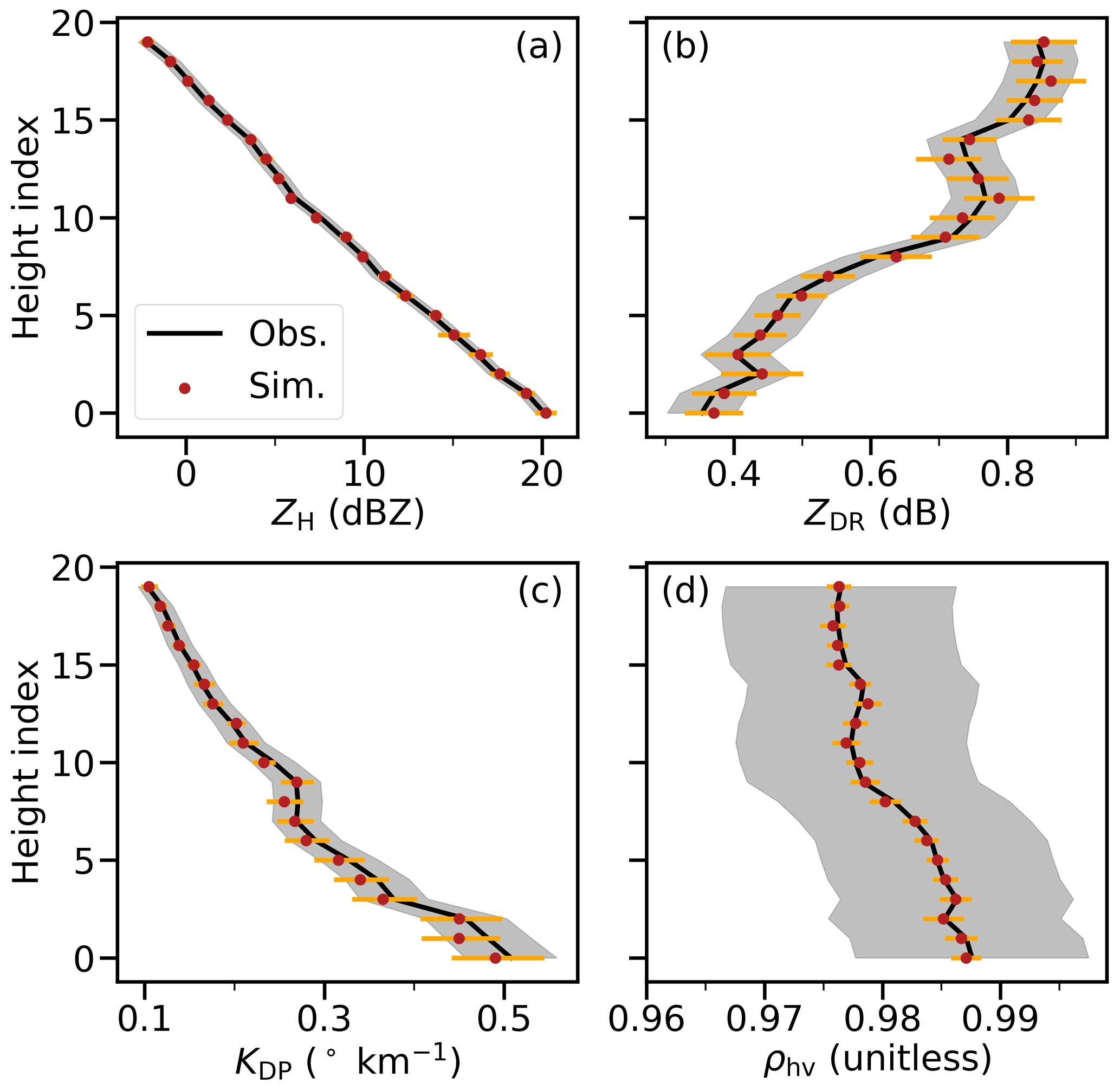
Figure 4 Profiles of (a) Z_H, (b) Z_DR, (c) K_DP, and (d) ρ_hv for synthetic observations (black line) calculated from the ice cloud properties given in Fig. 5 and for the mean of forward simulations from the ensemble (red dots). Grey shading denotes the observational uncertainties given in Table 3, while error bars in orange denote retrieval uncertainty calculated as the 1-standard-deviation spread of the ensemble simulations.

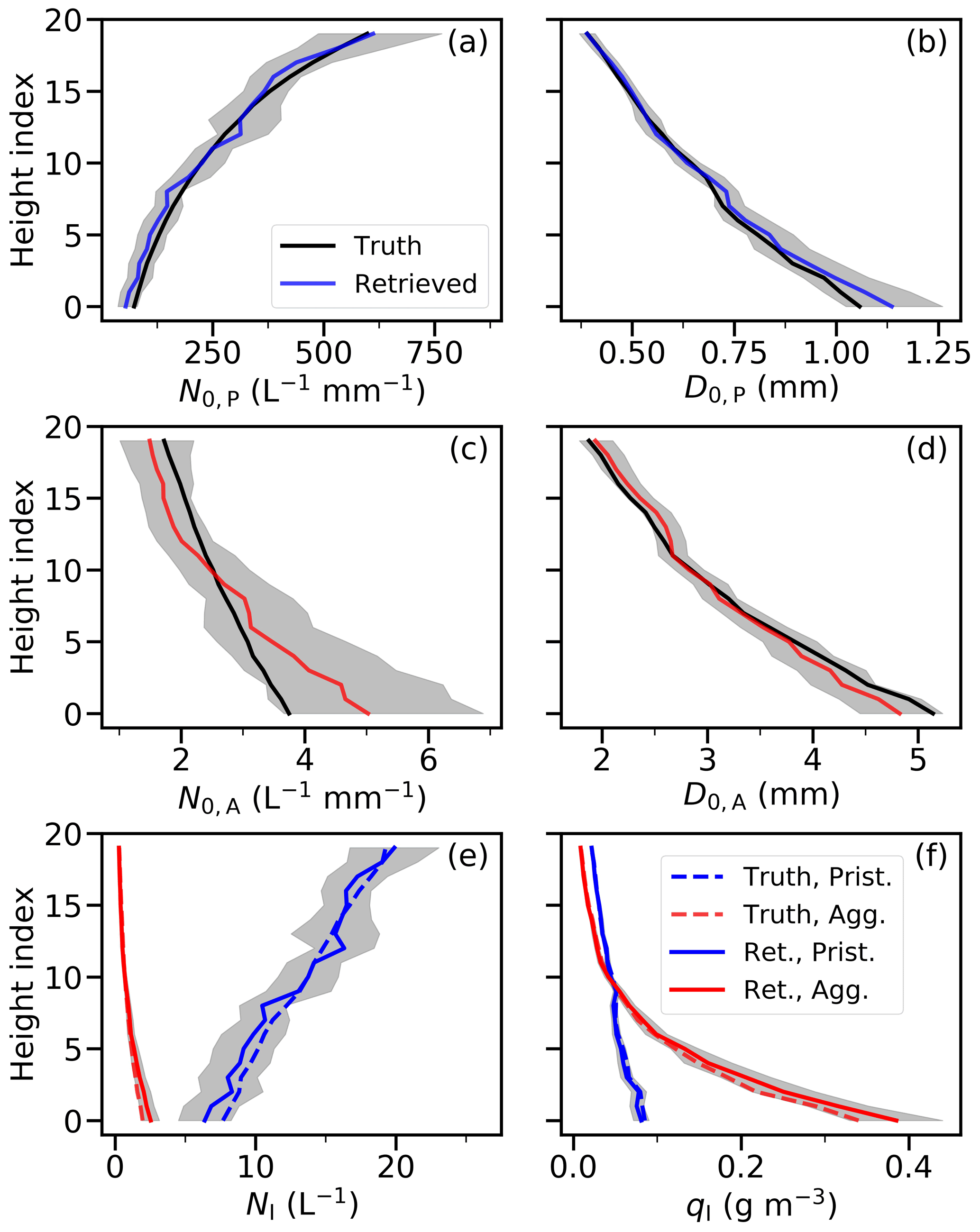
Figure 5 Profiles of (a) normalized number concentration and (b) normalization diameter for pristine ice and (c) normalized number concentration and (d) normalization diameter for aggregates. Panel (e) represents the total number concentrations, and panel (f) represents ice water contents of pristine ice and aggregates. Truth is denoted by solid black lines in (a)–(d) and by dashed lines in (e) and (f). The retrieved ensemble means are denoted by solid blue and red lines with shading that represents the 1-standard-deviation spread of the ensemble members. The habit of pristine ice is plate in this experiment.

Table 5 Truth means and the means, root-mean-square error (RMSE), and biases in retrieval in the synthetic dataset experiment.

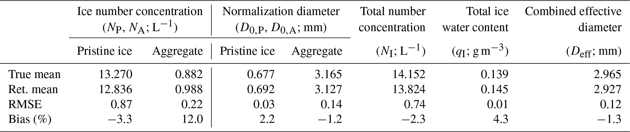
The forward-modelled observables of the ENCORE-ice solution in Fig. 4 agree well within the uncertainty in the synthetic values, providing confidence in retrievals. As shown in Fig. 5, the retrieval captures the vertical trend of the truth; the retrieval uncertainty estimated from the spread of the ensemble members also appears reasonable since the truth falls within the retrieval uncertainty. Because many combinations of N_0,A and D_0,A could lead to the same Z_H, we see some compensatory effects between N_0,A and D_0,A in aggregates at the lower layer. The errors are compensated for so that the error in the total ice water content is not enhanced, as shown in Table 5. Overall, the retrieval biases in the combined total number concentration, water content, and effective diameter properties are within 5 %, and the root-mean-square errors are small (see Table 5).

To conclude, this evaluation experiment demonstrates that the combination of these four radar observables is appropriate and the current observational uncertainty is sufficient for us to separate signals of pristine ice from aggregates. The errors in retrieved pristine-ice properties are small, and thus further physical interpretation based on the associated vertical profiles can be made to understand the underlying microphysical processes. For aggregates, the errors in retrieved size diameter and water content are small, but the vertical variations in retrieved number concentration may not follow the truth exactly due to the possible compensatory effects between number concentration and particle size.

4.2 Evaluation using PICASSO data

The case of 13 February 2018 from the PICASSO campaign represents a stratiform precipitating cloud system associated with a frontal passage. Using a radar scan at 08:37 UTC as an example, Fig. 6 shows a significant area with reduced ρ_hv, and enhanced Z_DR and K_DP at ∼ 3 km height, which suggests the presence of enhanced pristine ice embedded in snow aggregates. Based on the temperatures measured by the aircraft (Fig. 7), this area is in a temperature zone approximately between −12 and −18 ^∘C, and thus the preferred ice habit is likely to be dendrite and plate for this radar scan. During this radar scan, the FAAM aircraft was too far away to provide meaningful comparison, but cloud images showed that dendrites were present most of time during this period.

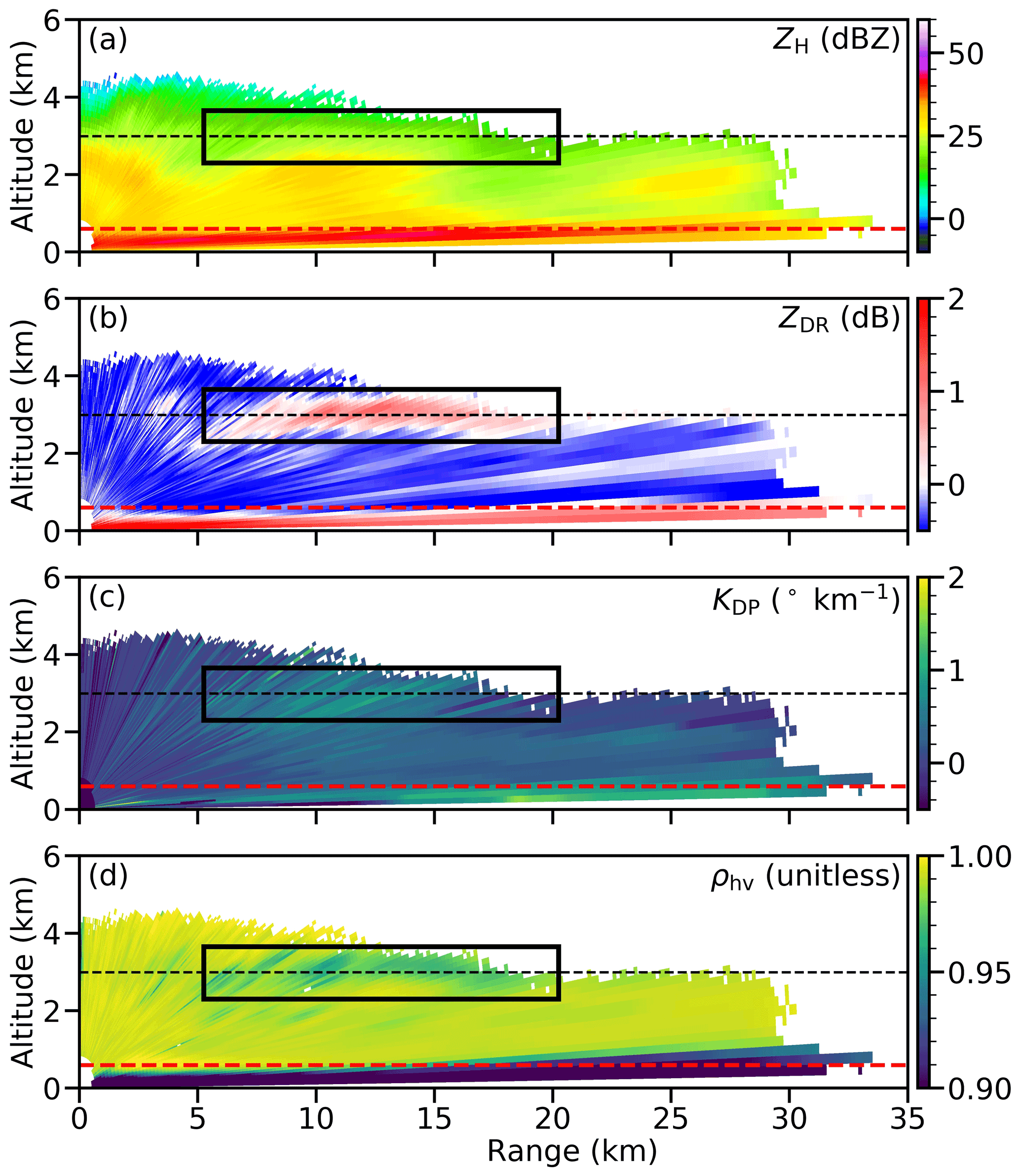
Figure 6 Height–range plots of observed (a) Z_H, (b) Z_DR, (c) K_DP, and (d) ρ_hv from the RHI scan at 08:37 UTC on 13 February 2018 during the PICASSO field campaign. The dashed red line denotes the 0 ^∘C level, while the dashed black line denotes the approximate flight altitude of the FAAM aircraft during the scan. The black polygon denotes the region that has enhanced Z_DR and K_DP and reduced ρ_hv.

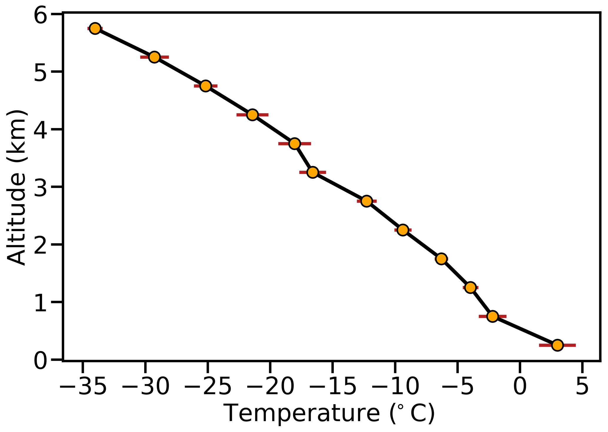
Figure 7 A temperature profile composited from aircraft in situ data during 06:00–09:00 UTC on 13 February 2018. Data between 06:33:30–06:39:20 UTC were unphysical and thus excluded. The error bars represent 1 standard deviation of sampled observations.

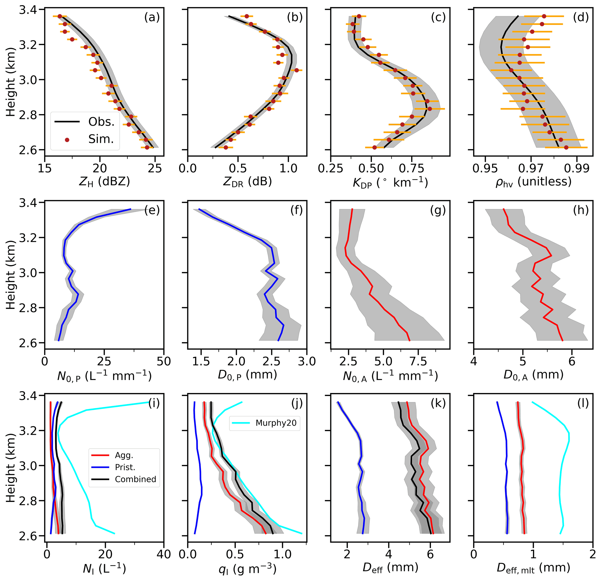
Figure 8 Retrieval performance for a radar ray at 08:37:39 UTC. Observed and forward-simulated profiles of (a) Z_H, (b) Z_DR, (c) K_DP, and (d) ρ_hv. The shading in (a)–(d) represents the observational uncertainty. The red dots represent the mean of the ensemble simulations, and the error bars represent 1 standard deviation in forward simulations. Panels (e)–(j) represent the retrieved mean normalized pristine-ice number concentration, pristine-ice normalization diameter, normalized aggregate number concentration, aggregate normalization diameter, the total number concentrations, and the total ice water content, respectively. Panels (k) and (l) represent the individual and combined effective mean diameters using the maximum particle dimension and the equivalent melted particle size as the size descriptor, respectively. The shading in (e)–(l) represents 1-standard-deviation uncertainty in retrieval. For comparisons, retrievals from Murphy20 are co-plotted in (i), (j), and (l).

Figure 8 shows detailed retrieval performance for a ray taken from the radar scan in Fig. 6. For this case, retrievals using the dendrite habit perform best; the habit suggested by our retrieval is consistent with observed particle images. As shown in Fig. 8a–d, the forward modelled radar observables agree well with the observed vertical profiles. The normalization diameters for pristine ice and aggregates ($D_{\mathrm{0},\mathrm{P}},D_{\mathrm{0},\mathrm{A}}$) are about 2.5 and 5–6 mm, respectively. Retrieved N_I is relatively constant at ∼ 5 L⁻¹, due to the opposite vertical variations between N_P (increasing with height) and N_A (decreasing with height). In contrast, q_I decreases with height from 1 to 0.2 g m⁻³ because both N_A and D_0,A decrease with height.

Compared to Murphy20 retrievals, a few findings stand out. Firstly, retrieved q_I profiles from the two methods follow each other closely. This is not surprising because both q_I profiles are largely constrained by the same Z_H observations. Secondly, the retrieved Murphy20 N_I is much larger than that from ENCORE-ice. These results suggest that Murphy et al. (2020) have attributed all radar signals to one species like our pristine ice. Due to the smaller size of pristine ice compared to aggregates, the retrieved Murphy20 N_I must be much larger than that of ENCORE-ice to make up for having the same q_I value. This also explains why N_I and q_I in Murphy20 retrievals have similar profile shapes. Considering that the observed ρ_hv is not close to 1, the attribution to single species is likely inappropriate, leading to a large error in ice number concentration, even though q_I may seem reasonable. Finally, D_eff,mlt, the effective mean diameter using the equivalent melted diameter as the size descriptor, from Murphy20 retrievals tends to be larger than that from ENCORE-ice. This is partly because Murphy et al. (2020) have used denser ice particles; i.e. both the pre-factor and the exponent in their mass–size relationship are slightly larger than our aggregates. Since D_eff,mlt depends on the assumed mass–size relationship, Fig. 8l is used for a qualitative comparison only.

Extending the evaluation from one ray to collocated data, a set of thresholds for matching space and time is needed. Since the enhanced area in Fig. 6 is about 15 km wide and 1 km deep, we use this scale as one of our criteria and consider in situ observations and radar gates collocated if their distance is within 15 km in the horizontal and 1 km in the vertical. The time difference threshold for collocation is set to be within 3.5 min because a pair of back-to-back radar RHI scans were performed every 7 min (see Sect. 2). These spatial and temporal thresholds lead to six clusters of radar scans for intercomparison, which comprise 105 rays with a total of 1675 gates. For a given ray, if the root-mean-square difference between the measured and the forward-simulated radar observable is greater than 0.1 dB in Z_DR, 0.1^∘ km⁻¹ in K_DP, or 0.01 in ρ_hv, we consider that the retrieval quality for the entire ray is poor and exclude all the retrievals. After this exclusion, 81 rays with 1237 radar gates remain for the evaluation. Most unsuccessful retrievals are likely due to an inappropriate prior. To make the retrieval method work for those unsuccessful cases, we may need to assume priors with different shapes of vertical profiles. Unfortunately, we do not have good knowledge of those shapes and will need to rely on future campaigns to help gather this information by taking frequent multiple-layer flights around the radar site.

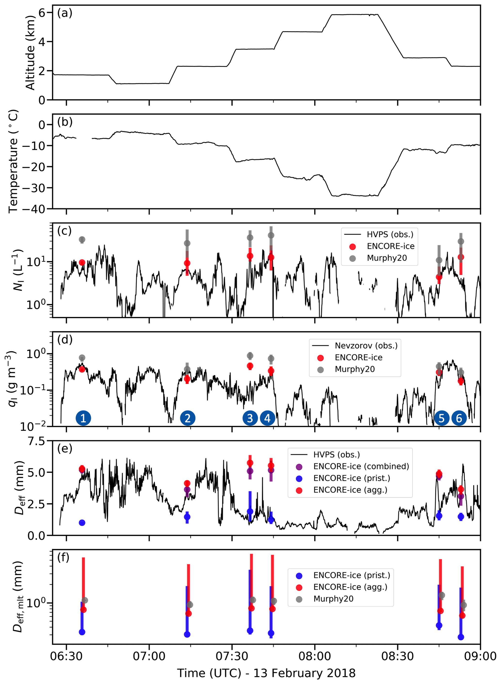
Figure 9 Time series of (a) flight altitude; (b) temperature; and observed and retrieved (c) total ice number concentration, (d) ice water content, (e) effective mean diameter using the maximum particle dimension as the size descriptor, and (f) effective mean diameter using the equivalent melted diameter as the size descriptor. Retrievals from ENCORE-ice and Murphy20 empirical relationships are denoted by dots, explained by detailed legends. The dots represent the median of retrievals from all collocated gates, and the vertical bars denote the range between the 25th and 75th percentiles. Note that the counting uncertainty in the total ice number concentration in (c) is plotted but too small to see. All calculations are based on the size range of HVPS observations, except Murphy20 retrievals in (c) and (d). For convenience, we index six retrieval clusters from 1 to 6 as shown in (d).

Figure 9 shows the time series of in situ observations and collocated retrievals. We expect column ice crystals at the beginning and very end of the time series because of the measured temperature higher than −10 ^∘C. The flight height was maintained at ∼ 2 km from 06:30 to 06:40 UTC, suggesting that the missing temperatures due to a data glitch at ∼ 06:40 UTC are likely to be about −5 ^∘C. During 07:10–08:45 UTC, the temperatures are between −10 and −20 ^∘C and likely favour the presence of both dendrite and plate. These expectations about prevalent ice habits are confirmed by visually checking the in situ cloud particle images (see Fig. 1 for examples).

In our retrievals, 40 % of the collocated radar observables are best fit with plate as the pristine-ice habit, 20 % with dendrite, and 40 % with columns. In general, when the cloud particle images were indeed dominated by columns, we have also found that retrievals with columns as the pristine-ice habit provide the best agreement between the measured and forward-simulated radar observables. In the period between 07:00–08:45 UTC when dendrites appeared much more frequently than plates in cloud particle images, our retrievals suggest the opposite because 40 % of best-fit retrievals are associated with plates and only 20 % of best-fit retrievals are associated with dendrite. Therefore, we consider that there remains a large uncertainty in distinguishing plate and dendrites using our retrievals. Note that even with this habit uncertainty, the choice of plate and dendrite does not lead to significantly different retrievals in N_I and q_I.

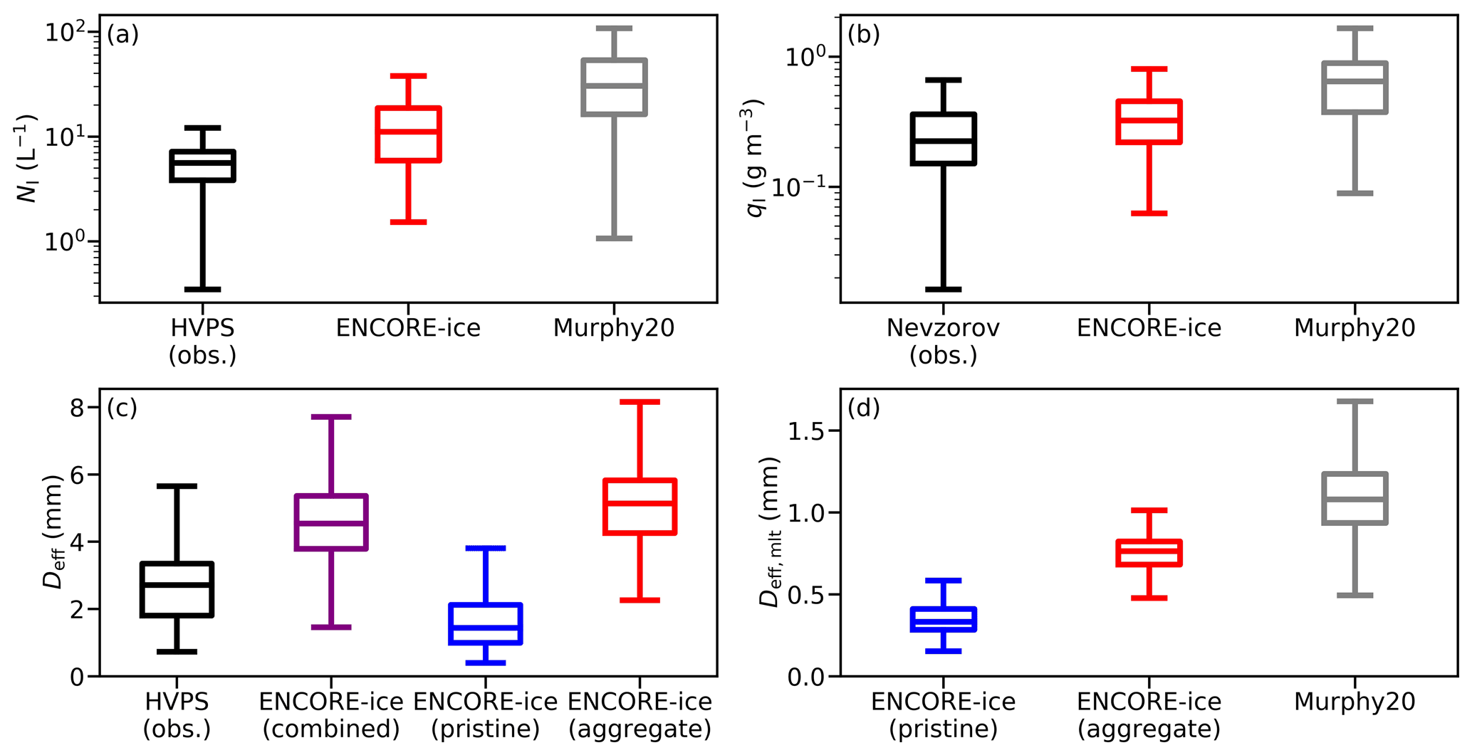
Figure 10 Box plots of in situ observations and retrievals from ENCORE-ice and Murphy20 for (a) total ice number concentration, (b) ice water content, (c) effective mean diameter using the maximum particle dimension as the size descriptor, and (d) effective mean diameter using the equivalent melted diameter as the size descriptor. The bottom and top of each box represent the 25 % and 75 % quartiles, and the line inside the box represents the median. The whiskers represent the range of data points within 1.5 times the interquartile distance. The included sample sizes for in situ data and radar gates are 347 and 1237, respectively.

The collocated retrievals in Fig. 9c and d show that N_I retrieved from ENCORE-ice is approximately on the same order of magnitude as observations and that the retrieved q_I values are close to the Nevzorov probe observations. N_I and q_I from ENCORE-ice generally perform better than those from Murphy20, but they are both overestimated as indicated by the box plots in Fig. 10. The overestimations in the median of N_I and q_I are 98 % and 44 %, respectively, for ENCORE-ice, and 445 % and 187 %, respectively, for Murphy20. Note that Murphy20 retrievals in N_I and q_I are based on empirical relationships derived from size bins between zero and infinity, while HVPS-based and ENOCRE-ice-based estimates are derived using HVPS size bins from between 75 and 19 275 µm. This difference in size ranges is not a concern for comparisons of q_I, but it contributes to part of the overestimation in N_I in Murhpy20 retrievals. Using our retrieved PSD, we have found that the median N_I derived from zero- and infinity-sized bins is ∼ 3 % larger than that derived from the HVPS size range. This suggests that the difference in the size range for integration calculations is not the main cause for the 445 % overestimation in Murphy20 N_I retrievals. Additionally, similarly to in Fig. 8l, Murphy20 D_eff,mlt tends to be larger than our D_eff,mlt from aggregates by 0.3 mm in the overall median, as shown in Figs. 9f and 10d.

Recall as per Eq. (6) that the effective mean diameter is weighted by size and thus strongly influenced by large particles. When observations sample both pristine ice and aggregates, the combined mean particle size is expected to be close to the size of aggregates, not pristine ice. The results in Fig. 9e generally match this expectation, showing a reasonable agreement between the observed and the combined mean diameter, except three data clusters during the period between 07:30 and 08:45 UTC. For Cluster 5 around 08:45 UTC, the D_eff from HVPS has a large variation, ranging between 1.4 and ∼ 5 mm with a median of 2.8 mm. This range is on the same order of the median D_eff of pristine ice (1.5 mm) and of aggregates (∼ 5 mm), though the median combined D_eff of 4.7 mm is significantly larger than the observed median. For clusters 3 and 4 between 07:30 and 07:45 UTC, the observed effective mean diameter is closer to the retrieved pristine-ice diameter. This unexpected behaviour might suggest a few scenarios, which are discussed in detail next.

The first scenario is that the radar volume might include pristine ice only or aggregates only. However, as shown in Murphy20 retrievals, assuming single species leads to a large error in N_P. The observed ρ_hv is also too low to support this scenario. The second scenario is that the separation between pristine ice and aggregates in our retrieval is inappropriate. To assess this possibility, we tested various combinations of N₀ and D₀ and found that the following two conditions must be met for the combined size to be close to the size of pristine ice. The first is that N_P needs to be at least 1 order of magnitude larger than N_A, and the second is that D_0,P cannot be much smaller than D_0,A. To meet the first condition, let us assume that our retrieved N_A is supposed to be 10 times smaller because our retrieved N_P from ENCORE-ice is already overestimated compared to the in situ observations and should not be even higher. Under that assumption, D_0,A needs to increase by a factor of 1.5 to maintain the same radar reflectivity observation. An increase in D_0,A, however, would make the difference between D_0,P and D_0,A even larger, which violates the second required condition. The combination of reduced N_A and increased D_0,A by the factors used above would also reduce q_I by a factor of 3. Then, to make up for the reduction in q_I, one can increase D_0,P to remediate the second required condition. This eventually leads to a scenario where two species are alike, as in the first scenario, which is not supported by the observations.

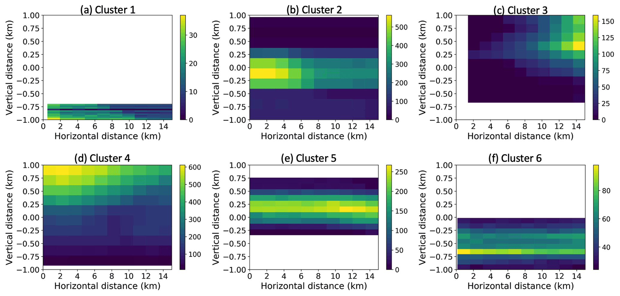
Figure 11 Two-dimensional histograms of occurrences of distances in the vertical and horizontal between in situ measurements and radar gates for Cluster 1–6 in (a)–(f), respectively. Note that occurrences are counted for all pairs of in situ data points and radar gates. In calculations of retrieval errors, selected in situ data points and radar gates are only used once with equal weights.

The third scenario is that the discrepancy in D_eff is due to a sampling issue. Figure 11 shows two-dimensional histograms of occurrences of the vertical and horizontal distance in the collocated in situ and radar dataset. The distance was calculated with respect to the radar gate; i.e. the positive vertical distance represents the flight altitude being higher than the radar gate of interest. Interestingly, for clusters 1, 2, and 6, in situ samples were taken largely at radar scan heights or below. It is likely that both aircraft and radar have sampled the same regime with notable aggregations, which explains why the observed D_eff is close to the retrieved D_eff of aggregates. In contrast, in situ samples were taken at higher altitudes over the radar scans for clusters 3–5. In these cases, aircraft may have sampled a pristine-ice growth zone aloft, but the radar gates below sampled the subsequent aggregations, which explains why the observed D_eff is closer to the retrieved D_eff of pristine ice, rather than of aggregates. Further studies using more datasets and retrievals would be needed to assess the third scenario. Overall, when including clusters 1, 2, and 6, the difference between the observed and the retrieved combined median D_eff is about 0.55 mm.

5 Summary

We have introduced a new method for retrieving microphysical properties of concurrent pristine ice and snow aggregates from X-band polarimetric radar observations. The radar observables used here include horizontal reflectivity, differential reflectivity, the co-polar correlation coefficient, and specific differential phase shift. The first observable provides constraints on the combined aggregate and pristine-ice population, while the last three observables provide constraints on the partitioning between aggregates and pristine ice, as well as on the ice number concentration and size of pristine ice. The observations are combined with our prior knowledge via an ensemble retrieval framework to find the best estimates of microphysical properties. Since properties of pristine ice and snow aggregates vary significantly in nature, we apply a widely spread prior, and thus the retrieval is mainly dominated by the observations.

Based on the evaluation using synthetic observations, we have found that the current observational uncertainty is sufficient for quantifying properties of pristine ice and snow aggregates. The retrieval was able to reproduce vertical profiles similar to the truth, and the root-mean-square error with respect to the truth is within the retrieval uncertainty. The biases in the combined total ice number concentration, ice water content, and effective mean diameter are all within 5 %. This exercise demonstrates that our retrieval method works well if the prior and the forward models for simulating radar observables are chosen appropriately and are representative of reality. In general, the appropriateness and representativeness of the prior and forward model can be confirmed by examining the agreement between the observations and the forward simulations.

We have also evaluated our retrieval against in situ cloud probe observations taken from a recent field campaign in Chilbolton, UK, which was coordinated to have collocated X-band radar scans and aircraft flights. We analysed a 3 h long case that had 1237 collocated radar gates. Although the period was not particularly long, the aircraft sampled ice particles in temperature zones from −5 to −35 ^∘C, allowing us to assess the retrieval performance for cases that are dominated by column, plate, or dendrite. The collocated in situ data have a median number concentration of 5.6 L⁻¹, ice water content of 0.2 g m⁻³, and 2.7 mm effective mean diameter. Compared to in situ medians, our retrieved total number concentration and ice water content are overestimated by 98 % and 44 %, respectively. This performance is generally better than that from empirical relationships, which has differences of 445 % and 187 % in the total number concentration and ice water content, respectively, with respect to the in situ medians. For the effective mean diameter, the in situ observations agree with our effective mean diameter combined from pristine ice and aggregate in three data clusters with a difference of 0.55 mm. In other clusters, the observed effective mean diameters agree better with the retrieved size of pristine ice, likely because the aircraft sampled pristine-ice growth zones aloft instead of the aggregation zones that the radar sampled. Since planar crystal growth and subsequent aggregation can lead to zones with distinct ice bulk properties, taking frequent aircraft measurements at multiple vertical layers around the radar location would be particularly helpful to improve collocations and allow us to analyse individual rays in more detail.

Currently, our method is designed to work for conditions with a mixture of pristine ice and aggregates. In the presence of rimed particles, the state vector should be expanded to include additional variables that can accommodate and inform the degree of riming, e.g. the riming factor described in Masson et al. (2018), or to include appropriate rimed species explicitly. When triple-frequency measurements are available and can be used to distinguish particle types effectively (e.g. Kneifel et al., 2015; Barrett et al., 2019), such information on particle types can also be incorporated into our method to provide retrievals for off-zenith radar scans that are more challenging for triple-frequency techniques. It is also possible to expand the observation vector with other radar observables at multiple wavelengths, providing further constraints on retrieval if added information exists.

This work is the first step towards quantifying microphysical properties of concurrent ice species, using a framework that considers our prior knowledge and the observational uncertainties. Since we have focused on radar signals with a reduced co-polar correlation coefficient and enhanced differential reflectivity and specific differential phase shift (i.e. cases with a potentially high ice number concentration), the immediate application will be to study dendritic growth zones commonly found in thick stratiform clouds. In particular, the Atmospheric Radiation Measurement (ARM) user facility has operated X-band polarimetric radars at fixed sites since 2011. Comprehensive X-band measurements from various scan strategies are also available from the Biogenic Aerosols – Effects on Clouds and Climate field campaign in Finland, which took place in 2014. These rich datasets will allow us to study formation of new crystals via either primary nucleation or a secondary ice process, their growth into planar crystals and dendrites, and the subsequent aggregations. The retrieved ice properties can be further compared to model simulations to understand what controls the ice number productions.

Appendix A

Radar equations for a single sample volume containing multiple ice particle habits are given as (Jung et al., 2010)

$$\begin{array}{}\text{(A1)}& {\displaystyle }\begin{array}{rl}{Z}_{\mathrm{h}}& ={\displaystyle \frac{\mathrm{4}{\mathit{\lambda }}^{\mathrm{4}}}{{\mathit{\pi }}^{\mathrm{4}}{\left|K_{\mathrm{w}}\right|}^{\mathrm{2}}}}\sum _{i=\mathrm{1}}^J\underset{\mathrm{0}}{\overset{\mathrm{\infty }}{\int }}\left\{\stackrel{\mathrm{‾}}{A{\left|S_{\mathrm{hh},i}^{\mathrm{b}}\right|}^{\mathrm{2}}+B{\left|S_{\mathrm{vv},\mathrm{i}}^{\mathrm{b}}\right|}^{\mathrm{2}}}\right.\\ & \left.\stackrel{\mathrm{‾}}{+\mathrm{2}C\mathrm{Re}\left[S_{\mathrm{hh},i}^{\mathrm{b}}{S_{\mathrm{vv},\mathrm{i}}^{\mathrm{b}}}^{\ast }\right]}\right\}n\left(D\right)\mathrm{d}D,\end{array}\text{(A2)}& {\displaystyle }\begin{array}{rl}{Z}_{\mathrm{v}}& ={\displaystyle \frac{\mathrm{4}{\mathit{\lambda }}^{\mathrm{4}}}{{\mathit{\pi }}^{\mathrm{4}}{\left|K_{\mathrm{w}}\right|}^{\mathrm{2}}}}\sum _{i=\mathrm{1}}^J\underset{\mathrm{0}}{\overset{\mathrm{\infty }}{\int }}\left\{\stackrel{\mathrm{‾}}{B{\left|S_{\mathrm{hh},i}^{\mathrm{b}}\right|}^{\mathrm{2}}+A{\left|S_{\mathrm{vv},\mathrm{i}}^{\mathrm{b}}\right|}^{\mathrm{2}}}\right.\\ & \left.\stackrel{\mathrm{‾}}{+\mathrm{2}C\mathrm{Re}\left[S_{\mathrm{hh},i}^{\mathrm{b}}{S_{\mathrm{vv},\mathrm{i}}^{\mathrm{b}}}^{\ast }\right]}\right\}n\left(D\right)\mathrm{d}D,\end{array}\text{(A3)}& {\displaystyle }\begin{array}{rl}{Z}_{\mathrm{hv}}& ={\displaystyle \frac{\mathrm{4}{\mathit{\lambda }}^{\mathrm{4}}}{{\mathit{\pi }}^{\mathrm{4}}{\left|K_{\mathrm{w}}\right|}^{\mathrm{2}}}}\sum _{i=\mathrm{1}}^J\underset{\mathrm{0}}{\overset{\mathrm{\infty }}{\int }}\left\{\stackrel{\mathrm{‾}}{C\left[{\left|S_{\mathrm{hh},i}^{\mathrm{b}}\right|}^{\mathrm{2}}+{\left|S_{\mathrm{vv},\mathrm{i}}^{\mathrm{b}}\right|}^{\mathrm{2}}\right]}\right.\\ & \left.\stackrel{\mathrm{‾}}{+A\left[S_{\mathrm{hh},i}^{\mathrm{b}}{S_{\mathrm{vv},\mathrm{i}}^{\mathrm{b}}}^{\ast }\right]+B\left[S_{\mathrm{vv},\mathrm{i}}^{\mathrm{b}}{S_{\mathrm{hh},i}^{\mathrm{b}}}^{\ast }\right]}\right\}n\left(D\right)\mathrm{d}D,\end{array}\text{(A4)}& {\displaystyle }{Z}_{\mathrm{dr}}={\displaystyle \frac{Z_{\mathrm{h}}}{Z_{\mathrm{v}}}},\text{(A5)}& {\displaystyle }{\mathit{\rho }}_{\mathrm{hv}}={\displaystyle \frac{\left|Z_{\mathrm{hv}}\right|}{{\left[\left(Z_{\mathrm{h}}\right)\left(Z_{\mathrm{v}}\right)\right]}^{\mathrm{1}/\mathrm{2}}}},\end{array}$$

and

$$\begin{array}{}\text{(A6)}& K_{\mathrm{DP}}={\displaystyle \frac{\mathrm{0.18}\mathit{\lambda }}{\mathit{\pi }}}\sum _{i=\mathrm{1}}^J\underset{\mathrm{0}}{\overset{\mathrm{\infty }}{\int }}\left\{\stackrel{\mathrm{‾}}{C_k\mathrm{Re}\left[S_{\mathrm{hh},i}^{\mathrm{f}}-S_{\mathrm{vv},\mathrm{i}}^{\mathrm{f}}\right]}\right\}n\left(D\right)\mathrm{d}D,\end{array}$$

where Z_h, Z_v, and Z_hv are in units of mm⁶ m⁻³; D is the maximum particle dimension; λ is the radar wavelength; K_w is the dielectric factor of water and ${\left|K_{\mathrm{w}}\right|}^{\mathrm{2}}=\mathrm{0.93}$; and the amplitude scattering matrix elements (S) are in units of millimetres. The vertical bars represent the magnitude of the terms within them, while Re represents the real part of the complex number, and the asterisk indicates its complex conjugate. The index i represents the species existing in the radar volume, and the index J represents the number of species. Note that the amplitude scattering matrix elements in the database are tabulated for various elevation angles, azimuth angles, and habit realizations. To apply these amplitude elements to Eqs. (A1)–(A6), $S_{\mathrm{hh}}^{\mathrm{f},b}$ and $S_{\mathrm{vv}}^{\mathrm{f},b}$ are first linearly interpolated with respect to elevation angles for radar rays. The interpolated $S_{\mathrm{hh}}^{\mathrm{f},b}$ and $S_{\mathrm{vv}}^{\mathrm{f},b}$ are then used to calculate the terms in the parentheses for all azimuth angles and habit variations. Because the azimuthal orientation of hydrometeors relative to the radar is random and unknown and because the exact morphological characteristics of these particles at any given time in nature are also unknown, the terms in the parentheses are averaged over azimuth angles and habit realizations, which are represented by the horizontal bar over the parentheses.

Coefficients A, B, C, and C_k are included to account for the effects of canting on the polarimetric radar moments. Following Jung et al. (2010) and Ryzhkov et al. (2011), the canting angle distributions are assumed to be Gaussian, and their effects can be parameterized using the mean and standard deviation of the distribution. Supposing that all oblate species fall with their major axes preferentially oriented in the horizontal plane, the mean canting angle can be set to zero (Ryzhkov et al., 2011). The width of the canting angle distribution is set to 10^∘ for pristine ice crystals and 60^∘ for snow aggregates, similarly to in Ryzhkov et al. (2011) and Matsui et al. (2019). All detailed equations and coefficients can be found in Jung et al. (2010).

Appendix B

Ryzhkov and Zrnic (2019) used a power-law dependence to describe particle density, given as

$$\begin{array}{}\text{(B1)}& \mathit{\rho }=\mathit{\alpha }{D}_{\mathrm{e}}^{-\mathrm{1}},\end{array}$$

where the density ρ is in g cm⁻³, coefficient α is in g cm⁻², and D_e is the equivalent volume diameter. They also assumed an exponential particle size distribution; i.e.

$$\begin{array}{}\text{(B2)}& N\left(D_{\mathrm{e}}\right)=N_{\mathrm{0},\mathrm{s}}{e}^{-\wedge D_{\mathrm{e}}},\end{array}$$

with an intercept N_0,s and the exponent ∧. From their Eqs. (11.32) and (11.33) in Ryzhkov and Zrnic (2019), we can calculate these two parameters by

$$\begin{array}{}\text{(B3)}& {\displaystyle }\wedge ={\displaystyle \frac{\mathrm{4}}{D_{\mathrm{emp}}}},\text{(B4)}& {\displaystyle }\mathit{\alpha }=\mathrm{0.00309}{\displaystyle \frac{Z}{q_{\mathrm{I},\mathrm{emp}}\cdot D_{\mathrm{emp}}^{\mathrm{2}}}},\end{array}$$

and

$$\begin{array}{}\text{(B5)}& N_{\mathrm{0},\mathrm{s}}={\displaystyle \frac{q_{\mathrm{I},\mathrm{emp}}}{\mathrm{0.0003811}\cdot {\mathit{\alpha }}^{-\mathrm{0.2}}{Z}^{\mathrm{0.6}}}},\end{array}$$

where the exponent ∧ is in mm⁻¹, N_0,s is in m⁻³ mm⁻¹, α is in g cm⁻², Z is the radar reflectivity in mm⁶ m⁻³, q_I,emp is the retrieved ice water content from Eq. (19) in g m⁻³, and D_emp is the retrieved diameter from Eq. (17) in millimetres.

Once N_0,s and ∧ are known in Eq. (B2), we further convert the size descriptor D_e to the equivalent melted diameter (denoted as D_mlt) by

$$\begin{array}{}\text{(B6)}& D_{\mathrm{mlt}}={\left({\displaystyle \frac{\mathit{\alpha }}{{\mathit{\rho }}_{\mathrm{w}}}}{D}_{\mathrm{e}}^{\mathrm{2}}\right)}^{\frac{\mathrm{1}}{\mathrm{3}}}\end{array}$$

and then calculate the effective mean diameter D_eff,mlt using Eq. (7).