An unmanned aerial vehicle sampling platform for atmospheric water vapor isotopes in polar environments

Above polar ice sheets, atmospheric water vapor exchange occurs across the planetary boundary layer (PBL) and is an important mechanism in a number of processes that affect the surface mass balance of the ice sheets. Yet, this exchange is not well understood and has substantial implications for modeling and remote sensing of the polar hydrologic cycle. Efforts to characterize the exchange face substantial logistical challenges including the remoteness of ice sheet field camps, extreme weather conditions, low humidity and temperature that limit the effectiveness of instruments, and dangers associated with flying manned aircraft at low altitudes. Here, we present an unmanned aerial vehicle (UAV) sampling platform for operation in extreme polar environments that is capable of sampling atmospheric water vapor for subsequent measurement of water isotopes. This system was deployed to the East Greenland Ice-core Project (EastGRIP) camp in northeast Greenland during summer 2019. Four sampling flight missions were completed. With a suite of atmospheric measurements aboard the UAV (temperature, humidity, pressure, GPS) we determine the height of the PBL using online algorithms, allowing for strategic decision-making by the pilot to sample water isotopes above and below the PBL. Water isotope data were measured by a Picarro L2130-i instrument using flasks of atmospheric air collected within the nose cone of the UAV. The internal repeatability for δD and δ¹⁸O was 2.8 ‰ and 0.45 ‰, respectively, which we also compared to independent EastGRIP tower-isotope data. Based on these results, we demonstrate the efficacy of this new UAV-isotope platform and present improvements to be utilized in future polar field campaigns. The system is also designed to be readily adaptable to other fields of study, such as measurement of carbon cycle gases or remote sensing of ground conditions.

1 Introduction

The Greenland and Antarctic ice sheets interact with the atmosphere through continuous exchange of water vapor by condensation and sublimation, as well as through precipitation events (Fettweis et al., 2020). The planetary boundary layer (PBL, the lowest layer of the troposphere directly influenced by the surface) generally has a thickness of tens to hundreds of meters above the ice sheet and exchanges water vapor with the free troposphere (FT) (Helmig et al., 2002; Galewsky et al., 2016). It is not clear how much water vapor is exchanged from surface sublimation flux, nor if the exchange ultimately results in a significant mass loss or mass gain for the ice sheet (Boisvert et al., 2017). The exchange of water vapor between the ice sheet and different parts of the atmosphere has importance for varying fields of study, including (1) ice–atmosphere modeling and mixing processes, (2) ice sheet mass balance, (3) satellite detection algorithms, (4) moisture tracking, (5) ice core science, and (6) modeling of the hydrologic cycle in general. In each of these cases, a critical missing component is the reliable measurement of the water vapor flux across the PBL border with the free troposphere. We hypothesize that atmospheric water vapor isotopes at altitudes within or above the PBL and especially in the few hundred meters above the ice sheet represents a measurable quantity, which allows us to quantify this flux.

Stable isotopes have been used to characterize the hydrological cycle since the first precipitation observations made by Dansgaard (1954). More recent studies have treated transport, phase changes, and other factors not available from precipitation records alone (e.g., Galewsky et al., 2016). For ice sheets, a common assumption that has persisted since early studies is that the isotopic composition of the ice sheets is solely informed by precipitation events. Yet, this assumption is being overturned with clear evidence that the ice sheet and the atmosphere constantly exchange water isotopologues with different rates leading to post-depositional change in the snow isotopic composition (Steen-Larsen et al., 2013, 2014a; Ritter et al., 2016; Hughes et al., 2021). This paradigm shift has not been fully accounted for in models, nor are these findings utilized for constraining ice-sheet–atmosphere interactions. This forms a substantial motivation for this study.

Early attempts to measure atmospheric water vapor isotopes were made by cryogenically trapping water vapor for subsequent analysis of the liquid, typically with mass spectrometers (Arnason, 1969) and over the ice sheet (Steen-Larsen et al., 2011; Landais et al., 2012). With the advent of laser-based isotopic instruments (Baer et al., 2002; Crosson et al., 2002; Gupta et al., 2009; Iannone et al., 2010), measurements in remote locations have become much more feasible, including the polar regions (Steen-Larsen et al., 2013; Bastrikov et al., 2014; Bonne et al., 2019; Leroy-Dos et al., 2021). A comprehensive listing of atmospheric water vapor isotopic measurements can be found in Wei et al. (2019). Direct measurements of water vapor isotopes collected from various elevations on small towers above the ice surface in Greenland (Steen-Larsen et al., 2013; Berkelhammer et al., 2016; Madsen et al., 2019) along with laboratory experiments (Ebner et al., 2017) have opened the pathway to understanding vapor transport and exchange with surface snow. In addition, satellite measurements (e.g., Worden et al., 2006; Frankenberg et al., 2009) and ground-based remote sensing data using spectra measured within global networks (Schneider et al., 2012, 2017; Rokotyan et al., 2014) offer greatly increased spatial coverage and typically measure the total atmospheric column. However, because of the different vertical sensitivities of ${{\mathrm{H}}_{\mathrm{2}}}^{\mathrm{16}}\mathrm{O}$, ${{\mathrm{H}}_{\mathrm{2}}}^{\mathrm{18}}\mathrm{O}$, and HDO of columnar retrievals, these data must be used carefully. So far, modeling based on water stable isotope observations of the exchange between the PBL and free troposphere has only been done for the marine boundary layer and only using ground-based observations (Benetti et al., 2018).

Bridging the two different scales of satellite remote sensing and in situ ground-based measurements is a challenging necessity for understanding the hydrologic cycle. Most efforts and testing have occurred at lower latitudes, far from the ice sheet. Franz and Röckmann (2005) developed a cryogenic sampler and protocol to collect stratospheric water vapor from very small mixing ratios (<10 ppm) flown on a C-17 aircraft during flights between New Zealand and Antarctica. In 2007, Strong et al. was successful in using pre-evacuated 650 cm³ glass flasks to collect atmospheric water vapor samples in the field and then cryogenically extracting the water and reducing it to hydrogen (Friedman et al., 1954), followed by mass spectrometer analysis. Vertical profiles were collected in approximately 300 m intervals using a light manned aircraft with a ceiling of 2–3 $\mathrm{km}\mathrm{a}.\mathrm{g}.\mathrm{l}.$ (above ground level) in the desert southwest of the US (Strong et al., 2007). As the engine of the aircraft was turned off during sampling in the Strong el al. study, obtaining airborne samples near the surface would be too dangerous.

There have been two recent measurement campaigns that utilized in situ optical water vapor isotope instruments to constrain remote sensing water isotope products. Herman et al. (2014) utilized a Picarro L1115-i CRDS analyzer across 27 flights by a Navion L-17a aircraft in the lower and mid-troposphere over the Alaskan boreal forest in a bias estimation study with the remote Aura Tropospheric Emission Spectrometer (TES). They estimated up to a +37 ‰ δD bias in the TES PBL estimate with a 20 ‰ uncertainty in that bias. Dryoff et al. (2015) flew seven profiles of δD with a CASA C-212 aircraft with the onboard ISOWAT-II instrument over the Canary Islands to triangulate between ground-based Fourier transform infrared (FTIR) spectrometer measurement and space-based IASI (infrared atmospheric sounding interferometer) during the MUSICA campaign (MUlti-platform remote Sensing of Isotopologues for investigating the Cycle of Atmospheric water). A validation study estimated a 40 ‰ uncertainty of δD in the lower troposphere and 15 ‰ in the upper troposphere against the FTIR product. Uncertainty in IASI was estimated by Schneider et al. (2015) to be 15 ‰ in the mid-troposphere with a +30 ‰–70 ‰ bias. Uncertainties of this magnitude are inadequate for constraining water vapor across the PBL and remain a target for improved methodologies.

We present results from a UAV pilot study at the East Greenland Ice-core Project (EastGRIP) site in northeast Greenland, occurring in summer 2019. We describe how customized UAVs can now be used to safely bridge satellite and ground-based measurements, all while overcoming the challenging polar conditions to sample atmospheric air in the low to mid-troposphere above the Greenland Ice Sheet. This is accomplished by designing an effective yet relatively inexpensive sampling platform with 3D-printed parts and accessible control devices on a commercially available fixed-wing UAV that collects air samples aloft for analysis immediately following flight with ground-based instrumentation. We show that water vapor isotope measurements can be achieved with sufficient precision relative to the magnitude of the observed gradient across the PBL and comparable with independent measurements made at the EastGRIP 10 m tower. We also demonstrate algorithmic methods of evaluating clustering indices of real-time onboard sensors to determine the altitude of the PBL, which can be used by the flight team to make informed sampling decisions mid-flight. We make recommendations for future field deployments to polar ice sheets and discuss the potential for how the observations can be used to improve the scientific understanding of varying fields of study.

2 Methods

2.1 Water isotope measurements

In this study, we made atmospheric water vapor measurements at the EastGRIP ice core field site in northeast Greenland (75.63^∘ N, 35.99^∘ W; 2700 $\mathrm{m}\mathrm{a}.\mathrm{s}.\mathrm{l}.$). A cavity ring-down laser spectroscopy (CRDS) instrument, model L2130-i (Picarro Inc., Santa Clara, CA), was used in conjunction with a custom inlet to introduce both samples and standards with equal treatment, described in more detail in Sect. 2.6. The standard water isotope data were analyzed on a continuous flow analysis (CFA) system adapted from Jones et al. (2017a). Results were validated against measurements made by the SNOWISO project (H2020 European Research Council Start Grant no. 759526), also using a Picarro L2130-i instrument (Sect. 2.3).

The data consist of measurements of hydrogen and oxygen isotopes in water vapor, where the ratio of heavy to light water isotopes in a sample is expressed in δ notation (Epstein et al., 1953; Mook and Rozanski, 2000) relative to internationally recognized primary reference materials Vienna Standard Mean Ocean Water (VSMOW) and normalized to Standard Light Antarctic Precipitation (SLAP) in accordance with IAEA reference material (2017):

$$\begin{array}{}\text{(1)}& {\displaystyle }{\displaystyle }{\mathit{\delta }}_{\text{sample}}=\left[\left({\displaystyle \frac{R_{\text{sample}}}{R_{\text{VSMOW}}}}\right)-\mathrm{1}\right]\times \mathrm{1000},\end{array}$$

where R is the isotopic ratio ${}^{\mathrm{18}}\mathrm{O}{/}^{\mathrm{16}}\mathrm{O}$ or D$/$H (i.e., ${}^{\mathrm{2}}\mathrm{H}{/}^{\mathrm{1}}\mathrm{H}$). The δD and δ¹⁸O symbols refer to fractional deviations from VSMOW, normally expressed in parts per thousand (per mill or ‰) . In practice, we maintain a suite of secondary reference waters that are rigorously calibrated to the primary reference materials (VSMOW and SLAP). Storage of our secondary reference waters is in accordance with methods described in IAEA technical note no. 43 (Newman et al., 2009).

2.2 EastGRIP hydrological cycle

The hydrological cycle on the Greenland ice sheet has several isotopic reservoirs and exchanges (Fig. 1). The dominant reservoir is the ice sheet, composed of ice, firn, and snow with a relatively positive water isotope value compared to the overlying atmosphere (Steen-Larsen et al., 2011). At the ice-sheet–atmosphere interface, both radiative (shortwave and longwave) and non-radiative (sensible and latent heat) energy fluxes occur, affecting the energy mass balance of the ice sheet. The summation of these processes leaves a diurnal imprint on the water isotopes in the upper few centimeters of the firn (Ritter et al., 2016; Madsen et al., 2019; Hughes et al., 2021). Within the PBL, turbulent mixing occurs with a magnitude largely dependent on stratification and wind shear. Significantly stable stratification of the PBL (e.g., during polar nights) may serve in part as a preventative mechanism of vapor leaving the ice sheet (Berkelhammer et al., 2016).

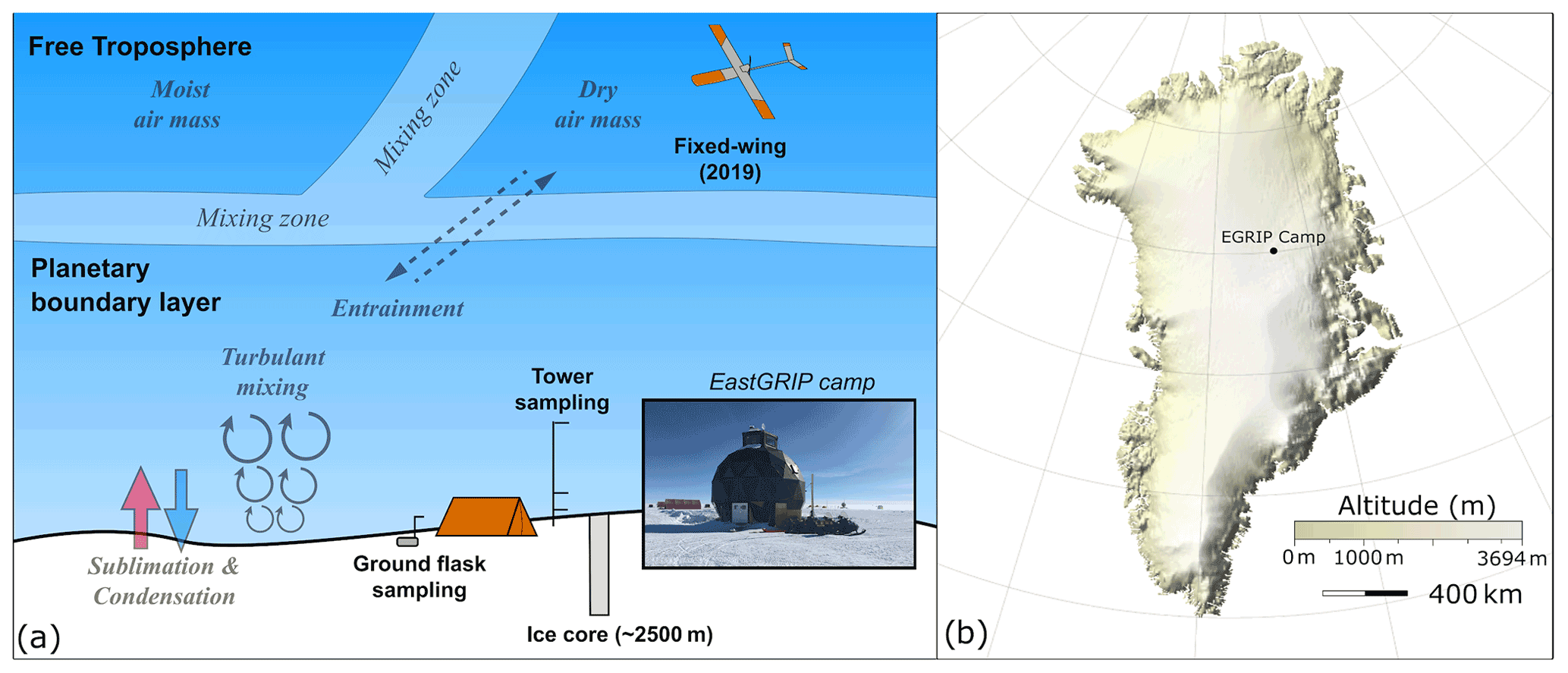
Figure 1 (a) Overview of the local hydrological cycle (excluding precipitation events) at the EastGRIP ice core camp. The water isotope sampling projects at EastGRIP in 2019 included ice core drilling, surface snow/ice sampling, continuous measurements of atmospheric air from a ∼7 m tower, and UAV sampling of atmospheric air. (b) Location of the EastGRIP ice core camp on the Greenland Ice Sheet at 75.6^∘ N, 35.9^∘ W (Wolfram Research, 2020).

At a constantly varying height above the ice sheet (tens to hundreds of meters in summer, lower in winter), a mixing zone between the surface and the PBL–free-troposphere boundary allows for entrainment of water vapor from the free troposphere into the PBL. This exchange is not well understood due to the inability thus far to make measurements across the full PBL (Boisvert et al., 2017). The inclusion of outside air parcels is mediated by synoptic changes in atmospheric general circulation (Schuenemann et al., 2009). Characterization of these synoptic-scale changes have been shown to be important to large-scale melt events, such as the 2012 event across the Greenland Ice Sheet where changes in atmospheric circulation resulted surface melt (Hanna et al., 2014). Due to the conservation of water isotopes through mixing, gradients in water isotopes across the PBL–free-troposphere mixing zone may provide evidence of the amount of water vapor exchange between air parcels. As UAV methodologies improve, it will eventually be possible to provide constraints on net exchange of water vapor across the PBL–free-troposphere interface.

2.3 EastGRIP tower measurements

During our UAV field campaign, simultaneous measurements of water isotopes were continuously taken at several heights above the snow surface. The tower setup used for these measurements was similar to the system described in Madsen et al. (2019). Four air intake inlets were installed at 0.5, 1.0, 2.0, and 7.1 m height above the snow surface, from which air was pumped to a Picarro L2140-i analyzer in a temperature-controlled tent ∼15 m away using an auxiliary pump.

In addition to documenting a diurnally varying water vapor isotope signal, the tower measurements have successfully been used to observe a gradient in the isotopic concentration in the lowest part of the PBL (Ritter et al., 2016; Madsen et al., 2019). This gradient has been used to argue that the exchange between the atmosphere and snow surface is driving the diurnal water isotope variations. Extending beyond tower heights will allow for the observation of entrainment processes and a better understanding of the formation of the ambient isotopic composition.

2.4 Fixed-wing UAV flight system

While at the EastGRIP camp in 2018 the team performed a proof of concept for airborne sampling and surface analysis using a small remote-controlled sampling package and a multi-rotor UAV (DJI S-1000, DJI, Inc.). The system was able to obtain data and samples for analysis up to 400 $\mathrm{m}\mathrm{a}.\mathrm{g}.\mathrm{l}.$, but navigation and control were very problematic, due to proximity to the magnetic pole and batteries at low temperature limiting flight times to less than 15 min. Knowing that sampling was possible and effective, we moved our attention to fixed-wing platforms that fly longer, fly higher, and are more stable to operate.

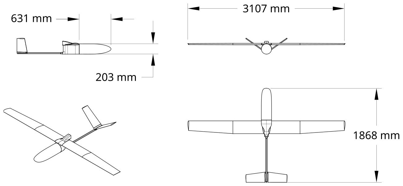
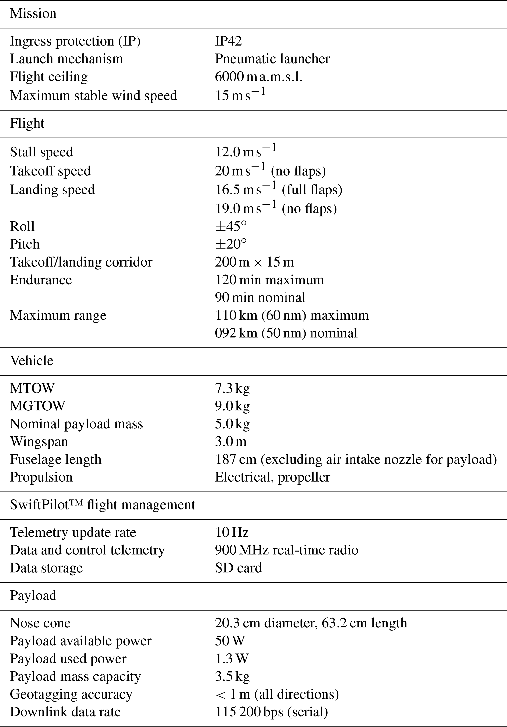
The S2 fixed-wing aircraft was the chosen platform for the 2019 campaign. The S2 is a modular, autonomous aircraft designed by Black Swift Technologies, LLC (BST) for science missions, based on simple-to-operate electric propulsion aircraft with a modular payload. It includes a lightweight composite airframe design (Fig. 2). The S2 is capable of conducting fully autonomous flights in unimproved areas such as an ice sheet in part due to its pneumatic launch system. The aircraft can adjust to changing wind conditions in real time, ensuring a high degree of stability for predefined mapping or atmospheric sampling applications (Elston et al., 2015). The aircraft can carry up to a 3.5 kg payload for up to 90 min. At arctic temperatures with the payload used in this study, we found 45 min of flight time typical and apt for climbing 1600 m and including needed sampling time. The broader technical specifications for the S2 are listed in Appendix C. A typical flight day including sampling is found in Sect. 2.8.

Figure 2 Overview of the S2 fixed-wing aircraft.

SwiftPilot™ (Black Swift Technologies, Boulder, CO) is a miniaturized autopilot system developed specifically for UAV applications, allowing for remote operation and autonomous operation monitoring with capability for intervention, and was used in this study. Its modular CAN-bus architecture enables a large number of connectivity options, simplifying payload integration into the processing stream. Communication with the ground is enabled through the SwiftStation™ (BST), a portable tripod-mountable ground station (1.8 kg) that supports user-specific sensor payload integration, downlink, waypoint programming and digital terrain model custom inputs, and operation control. The standard configuration, used in this study, contains a 3 dBi gain 900 MHz dipole as well as a GPS antenna.

2.4.1 Nose cone sampling pod

The flask sampling apparatus is contained within the nose cone, and a schematic of the system is shown in Fig. 3. The payload is suspended on four carbon fiber rods spaced 140 mm×80 mm apart which slide into the frame of the main aircraft, where a manufacturer-supplied baseplate secures the payload in place with two spring-loaded latches. We explored and tested the efficacy of holding water vapor within Teflon, Tedlar, and stainless-steel bags, and we observed memory effects in all three of those options. As such, eight glass flasks (Precision Glassblowing, Denver, Colorado) are suspended with memory foam in a series of modeled and 3D-printed nylon-12 plates (KODAK Nylon 12). Due to 12 G launching force from the pneumatic launching process, we found foam and the elastic properties of nylon-12 to be critical for flask safety. The printing was done on a XYZprinting da Vinci Super and sliced at a 15 % hex infill with XYZware Pro. The glass flasks are approximately 181 g each, are 500 cm³ in volume, and include a supported dip tube to ensure the sample is adequately flushed during fill. A series of $\mathrm{1}/\mathrm{4}$ in. o.d. Bev-A-Line V tubing (Cole-Parmer) connects the glass flasks to a common inlet and outlet aluminum manifold (SMC, model SS073B01-08C) fitted with 12 V DC solenoid valves (SMC, model S070B-6AC-M). The total weight of the sample pod is ∼2.3 kg. Air samples are loaded into the glass flasks during a 5 min flushing with air pulled from the intake port on the nose cone through the manifold and the selected flask to the diaphragm pump (KNF model DC-B 12V UNMP850). The pump is rated at 8 L min⁻¹, but with altitude and system restrictions the flow rate is reduced to ∼5 L min⁻¹, yielding approximately 50 flask volumes of flushing over the 5 min flush–fill process for each sample. Inlet and outlet valves are closed simultaneously so that flasks are not pressurized and remain at the ambient pressure of sampling. One of the extra valves is used for purging the manifold during sample analysis (see Sect. 2.6).

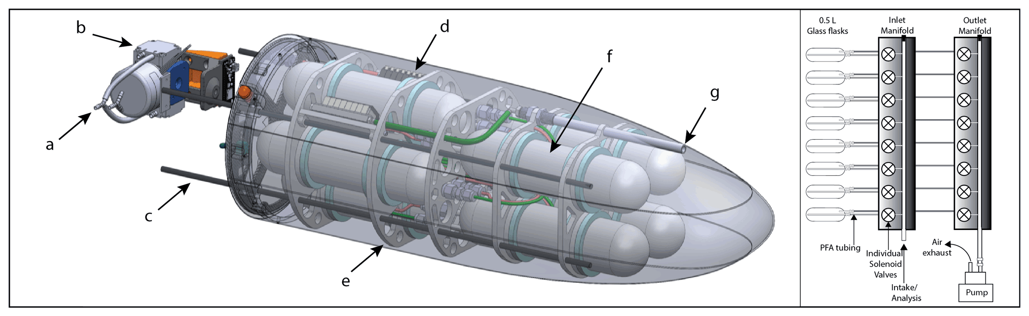
Figure 3 Left: overview of the custom nose cone sampling pod. (a) Air exhaust to outside the fuselage. (b) 8 L m⁻¹ KNF pump. (c) Supporting rods for payload connection to UAV fuselage. (d) Eight-port valve manifolds to inlet and outlet. (e) Nylon-12 baseplates with memory foam for flask suspension. (f) 500 cm³ glass flasks with a two-port dip tube. (g) Air intake. Right: schematic diagram of the same nose cone sampling pod, showing flow path of air from intake manifold, through flasks to outlet manifold and pump air exhaust.

2.4.2 Measurement scheme

Similar sample pod control systems were used for both airborne and ground sampling. For sampling during flight, the onboard microcontroller (Adafruit Feather M0) works through the BST SwiftCore™ flight system to communicate to the ground station. Payload control is managed by a laptop with Linux (Ubuntu 18.04.2) connected over Wi-Fi to the ground station. The microcontroller receives and manages commands to toggle valves and enable pumping. Environmental sensing is also fed into the BST SwiftCore™ and down to the ground station. The temperature and humidity is determined by an E + E Elektronik EE03-FT9 sensor (±0.3 ^∘C and ±3 % RH), and the pressure is determined by a high-resolution (±1.5 mbar) MEMS sensor (TE Connectivity MS5611). Both sensors are included as part of the forward-pointing package to assist in autopilot flight on the underside of the right wing of the aircraft to minimize solar radiation, a well-known issue with UAV applications (Greene et al., 2019). A detailed physical description of the sensor can be found in E + E Elektronik (2021). While underwing sensor placement may protect against top-down solar radiation, surface albedo is high over the Greenlandic ice sheet and may contribute to an unknown positive bias in measurement (Box et al., 2012).

In addition to measurements of samples taken during flights, a small (2 m) sampling tower was used for flask sampling to provide an additional near-surface data point and also allow an intercomparison with tower measurements of water vapor isotopes at EastGRIP. On the ground, a second microcontroller was connected to the sample pod with a USB cable. Its tasks included (1) controlled functions flushing dry air through flasks prior to flight, (2) sample acquisition from the 2 m tower, and (3) computer-controlled release of samples for isotopic analysis. Flasks from both flights and ground sampling are introduced to an L2130-i Picarro instrument for isotopic analysis by opening a single port on the flask. Before air sample ports are opened, dry air is plumbed into a spare valve at the back of the manifold to push out atmospheric air left in the manifold. In this manner the Picarro analyzer is pulling the sample air from the dead end of the flask, reducing the pressure slowly over time. Air samples are pulled from the flask into the instrument via the common port of the manifold at 30 sccm for approximately 12 min. Pressure within the analyzer cavity is carefully controlled at 50 Torr by the instrument with high-speed PID-controlled valves on both ends of the cavity. As water vapor is introduced to the CRDS cavity, isotopic mixing with the previous dry air parcels can affect the instrument's response to new samples. To address this, the first 3 min of observation for any one sample is cropped from averaging. Additionally, to address any issues associated with any reductions in flask pressure near the end, the last 3 min is also cropped. These timings were empirically derived from consistent plateaus of both isotopes and water concentrations between the beginning and ending tails. Cropping in this way also allows a mixing ratio/specific humidity to be determined for calibration. Values for any one sample are determined from the average over approximately 6 min. For a systematic diagram of the drone and ground sampling, see Appendix A.

The methods insured equal treatment of samples collected in flight or on the ground. This served two purposes: (1) to establish the isotopic bottom end-member of the vertical profile and (2) to enable the comparison of the sample pod measurements with the established in situ tower measurements of water vapor concentration and isotopes (Picarro L2140-i), taken at the same time within a distance of 10 m.

2.5 Water vapor isotope measurements and calibration

Systems have been developed by numerous groups to calibrate Picarro CRDS instruments used in continuous flow applications (Gkinis et al., 2011; Steen-Larsen et al., 2014b; Jones et al., 2017a), and each represents an evolution in design and performance. Due to the proven success with multiple measurement campaigns completed on ice cores with the calibration setup described in Jones et al. (2017a), we used the same principles in this setup for the calibration of the system in the field. It meets the ideal criteria for a calibration system as described in Bailey et al. (2015), which includes (a) enabling the introduction of low volume mixing ratios for calibration, (b) mitigating standard drift, and (c) utilizing multiple water standards in the calibration scheme. The system schematic is shown in Fig. 4.

Figure 4 System diagram of the inlet system that introduces water vapor from a suite of isotope standards or from glass flasks in the nose cone sample pods.

A Valco six-port stream selector valve (Valco Instruments Co. Inc.) controls selection of water standards in 30 mL Pyrex glass vials fitted with a $\mathrm{1}/\mathrm{16}$ in. capillary and a pigtail vent tube. The selected water standard is introduced to the flash evaporator system through a concentric nebulizer (Meinhard, TL-HEN-150-A0.2), powered by high-pressure (80 psi) dry air. The nebulizer inducts the water at 160–250 µL min⁻¹ and converts the liquid to a fine spray of approximately 1.5 µm droplets inside a 20 cm×1.8 cm diameter Pyrex tube heated to 200 ^∘C by a surrounding ceramic tube furnace (Watlow, VC400N06A). The spray is mixed with a separate flow of compressed dry air at 3.5 L min⁻¹ to achieve a vapor concentration of approximately 20 000 ppm. At the end of the furnace tube is an open-split-style intake line (Swagelok $\mathrm{3.175}\mathrm{mm}\mathrm{o}.\mathrm{d}.\times \mathrm{2}\mathrm{mm}\mathrm{i}.\mathrm{d}.\times \mathrm{10}$ cm stainless-steel tubing) inserted approximately 5 cm into the Pyrex furnace tube. Excess water vapor from the open split then vents to the room. Additional dry air (<50 ppm H₂O) is then introduced through a mass flow controller (Alicat Scientific, MC-100SCCM-D/5M) into the output line to further dilute water vapor down to desired concentrations necessary for calibration. At this stage, a manual three-way valve selects either the vapor output of the calibration system or selected glass flasks of the sample pod to enter the CRDS system. Control of the sample pod valves is coordinated with the microcontroller and the CRDS computer. The flow rate into the CRDS analyzer is approximately 30 sccm and controlled by a critical orifice inside the instrument and a pump (Vacuubrand MD1) attached to the Picarro L2130-i.

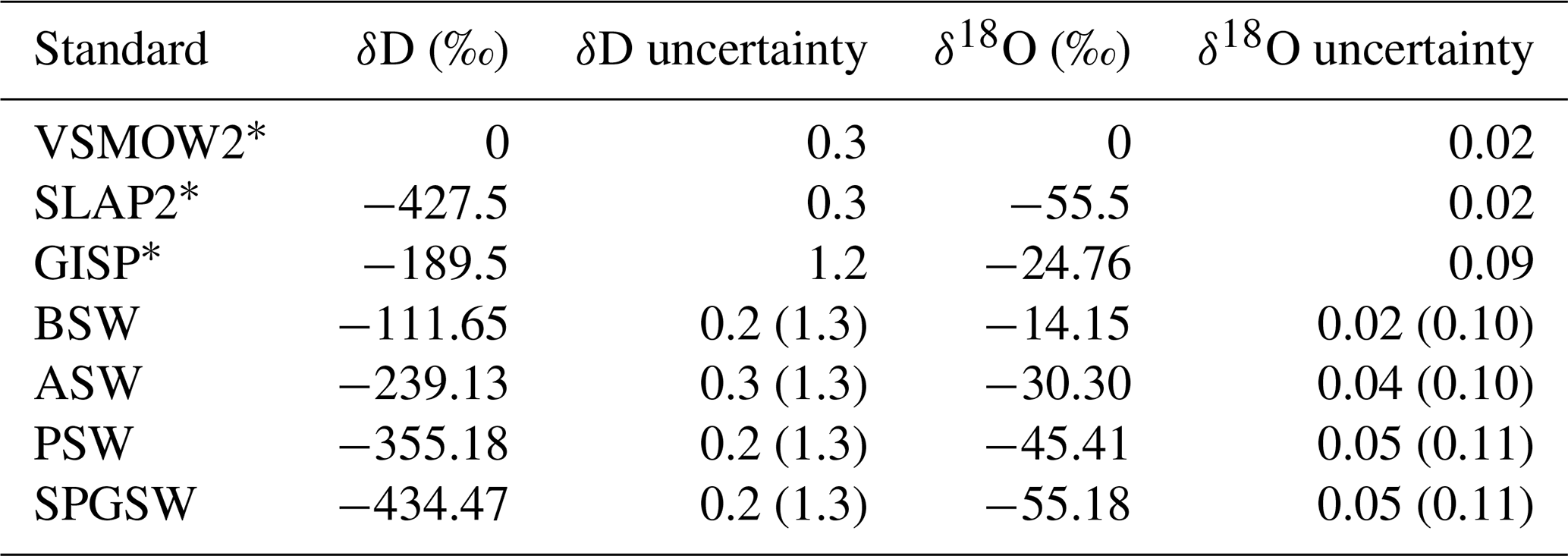
Raw values from the CRDS system are corrected in post-processing and tied to known values of isotopic water standards and corrected for the instrument's response to humidity. This is required because our atmospheric water vapor samples (typically <5000 ppm H₂O) are outside of the standard operating range of the Picarro L2130-i, which is optimized for the analysis of liquid water samples (10 000 to 25 000 ppm H₂O). Counting statistics for CRDS instruments are heavily dependent on sufficient concentration of gas species warranting calibration across a range of humidities and isotope standards. The isotopic water standards and their uncertainties are given in Table 1.

Table 1 Tracing of uncertainties is provided for primary reference water standards (^*) and secondary water standards developed in the laboratory, which are reported in units of per mil. The four secondary standards (BSW, ASW, PSW, and SPGSW) are previously calibrated in the laboratory and are defined relative to the primary standards (VSMOW2, SLAP2, and GISP) on which values and uncertainty are reported by the IAEA. Secondary standards are reported with uncertainty determined across multiple IRMS and CRDS platforms. In parentheses is the combined uncertainty of both the primary and secondary standard tie, added in quadrature. Additional details describing the calibration scheme can be found in Jones et al. (2017b).

To characterize the instrument's isotopic response to different water vapor concentrations, suites of measurements for each water standard are made under a range of humidities, from 500 to 25 000 ppm water vapor. This is accomplished on the system by adding measured amounts of additional dry air to the open-split vaporizer that feeds the instrument. Dry air was provided by one of two sources: a dry air generator (model CDA-10 by Altec Air, Broomfield, Colorado) that produced 10 L min⁻¹ air at −73 ^∘C dew point or dry air from a size 300 compressed air tank (zero grade, Airgas, USA). Both were capable of supplying air with less than 50 ppm H₂O. A mass flow controller (Alicat model MC-100SCCM-D) metered dry air to achieve a suite of desired humidities for calibration purposes. The resulting data were used to create an interpolated surface (Hermit Interpolation, Mathematica) of measured vs. adjusted, or true, isotopic values.

This calibration procedure was done several times throughout the 2019 field season to capture long-term instrument noise in response to humidity. Atmospheric samples were calibrated to the set of humidity measurements closest in time, ranging from as long as 7 d apart but typically 1–3 d throughout the season. Steen-Larsen et al. (2013) indicate that correctable linear drift may occur local in time to the measurement period due to strong diurnal temperature changes around the instrument. Because humidity calibrations were not regular about each measurement at the timescale of diurnal temperature change, the correction was not performed in this study. Future campaigns will include a higher calibration density to account for this.

2.6 Uncertainty in sampling and intercomparison with on-site water vapor tower

Outside of CRDS instrument performance, the UAV sampling system itself introduces sources of error. This uncertainty is associated with acquisition and transport of the sample water vapor as well as environmental change during the flight period. To understand the uncertainty in captured water vapor during the 2019 season, two different flask pod intercomparisons were performed in conjunction with the separate 2 m tower-isotope setup detailed in Sect. 2.3. For the intercomparison, each of the six flasks from three different sample pods was flushed with air from 2 m altitude for 5 min. As a total of 18 flask measurements correspond with an hour and half of sampling, this test is sensitive to changes in atmospheric water vapor isotopic composition. A more appropriate test would be to produce standardized water vapor as described in Sect. 2.5 and sample from that stream. This is challenging because the most accurate test would be to produce water vapor at a rate that can match the 5 L min⁻¹ sampling throughput of the pump, which is currently unachievable due to limited amounts of water standards. Though sampling was performed over this longer period of time without standard water vapor, the highest 1σ standard deviations of any one pod were of 0.45 ‰ in δ¹⁸O and 2.80 ‰ in δD. These values can be seen as the pessimistic view of uncertainty due to the non-ideal sampling situation but are reasonable given that previous uncertainty estimates on in situ water vapor isotope measurements range from 0.14 ‰ in δ¹⁸O and 0.85 ‰ in δD (Steen-Larsen et al., 2014b) to 0.23 ‰ in δ¹⁸O and 1.4 ‰ in δD (Steen-Larsen et al., 2013) depending on the environmental conditions.

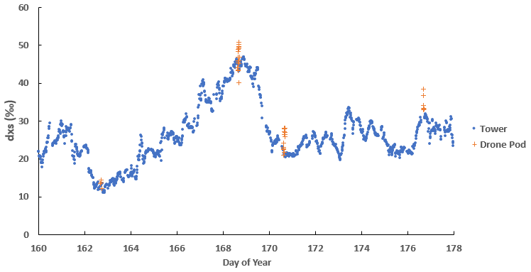
Figure 5 Comparison in second-order parameter dxs between the tower setup present at the EastGRIP camp in 2019 and 2 m pod intercomparison measurements. Drone pod measurements on 163 DOY (day of year) and 176 DOY correspond to flask measurements taken at 2 m during a flight mission. All measurements from both tower and UAV are tied to the same isotopic water standards listed in Table 1.

A comparison of UAV and tower deuterium excess (dxs) data is shown in Fig. 5. Deuterium excess is defined by Dansgaard (1964) as $\text{dxs}=\mathit{\delta }\mathrm{D}-\mathrm{8}{\mathit{\delta }}^{\mathrm{18}}\mathrm{O}$. The dxs is a more sensitive intercomparison metric than δ¹⁸O and δD and will more clearly show discrepancies between different measurement schemes. An intercomparison was done at four different times: (1) during 2 m sampling during two different flights and (2) during two different pod intercomparison measurements at 2 m. There is general agreement for dxs across the two platforms with a slightly more positive value for the UAV-isotope system. The positive relation is seen in both δD and δ¹⁸O, implying that the positive bias is due to an interplay of both measurements. Figures of separated δD and δ¹⁸O can be found in Appendix A.

2.7 Boundary layer prediction

During the 2019 field campaign, we used environmental measurements (pressure, potential temperature, specific humidity) taken in real time during each flight to evaluate Euclidean distance in the measurement domain to infer where the PBL–free-troposphere transition occurs in the spatial domain (Appendix D). The results were used by the pilot to make in-flight decisions about sampling altitudes for isotopic analysis. After the 2019 field campaign, we explored additional PBL identification algorithms. The PBL and free troposphere are largely decoupled, allowing for cluster density evaluation to determine the PBL height (Krawiec-Thayer, 2018). As the PBL structure varies in shape and magnitude for any one observational parameter, other methods such as gradient interpretation of single environmental variables are less useful (Krawiec-Thayer, 2018). The most promising algorithm, the Calinski–Harabasz criterion index (CHCI), is explained in Appendix D. The global maximum of this index is assumed to be the height of the PBL. The Calinski–Harabasz criterion index will be utilized in future field campaigns to detect the PBL in real time during flight in addition to user judgment. An example of the CHCI for PBL height determination is shown in Fig. 6.

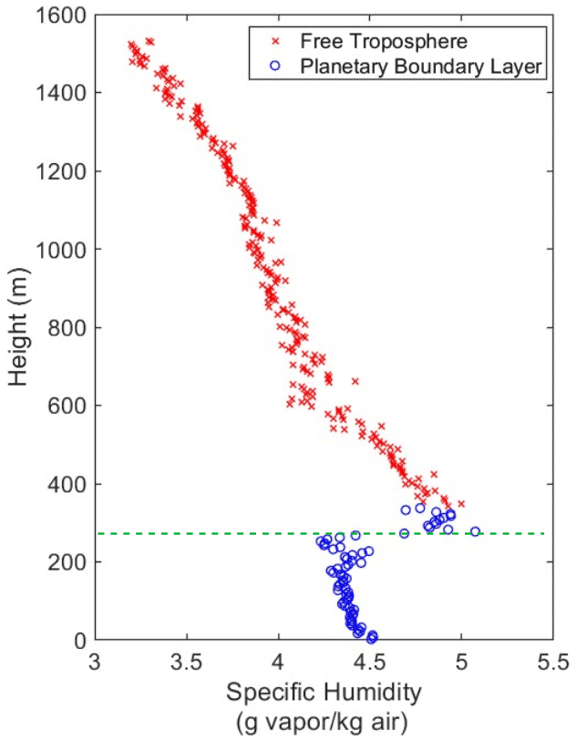
Figure 6 The Calinski–Harabasz criterion index (CHCI) applied to the sampling flight on 12 June with a priori assumption of K=2. Groups are assumed to represent the free troposphere and PBL, though more structure may exist. The boundary at ∼325 m using CHCI is not in agreement with that determined using the Euclidian distance in Fig. 7, which shows a likely boundary at ∼275 m. This value was chosen by the operator of the flight and shown as the dashed green line. Figure 10 shows an example of a failure in Euclidian distance to predict the boundary layer. The use of CHCI improves the PBL prediction algorithm, as determined in this study.

2.8 Typical analysis day and sample acquisition

Before flight is considered, the local weather is evaluated to determine the potential for mission success. To prevent potential icing, a nearby ceilometer (Vaisala Ceilometer CL31, Vaisala, Boulder, Colorado) present at the EastGRIP camp was used to safely determine that cloud cover was significantly higher than the highest flight altitude in the flight plan. Flights were not performed during precipitation events. Acceptable wind speeds were considered less than 10 m s⁻¹, two-thirds of maximum wind operation of 15 m s⁻¹ for the Black Swift S2 aircraft.

For any given analysis flight, a sequence of steps are completed to ensure quality control: (1) calibration of the water isotope measurement system (Sect. 2.6), (2) ongoing isotopic measurements at a 2 m tower during the flight (Sect. 2.7), (3) identification of the PBL during flight using real-time temperature and R$/$H from the aircraft (Sect. 2.8), (4) atmospheric sample acquisition during flight, and (5) isotope measurement following the flight, in a heated field tent (Sect. 2.6).

A calibration of the Picarro L2130-i is performed close to the time of flight. Before a flight, both ground-based and UAV-based glass flasks are flushed with dry air (75 ppm water vapor) for 10 min. Before launch (time permitting), an extra 2 m measurement is taken with the ground sampling system detailed in Sect. 2.5.2. After launch, the pilot ascends at an autopilot-controlled rate of 2 m s⁻¹ in a circular pattern (a 60 m diameter orbital). The ascension rate can be affected by local wind speeds requiring a slower vertical climb than the UAV is otherwise capable of. While a faster ascension is possible, a slower climb also minimizes hysteresis for the atmospheric sensors aboard the UAV. At the top of the climb, the aircraft automatically enters a holding orbital pattern at constant altitude while the operator assesses the real-time algorithmic determination of the PBL. The operator then inputs the altitude of the sampling locations for water isotopes above and below the PBL.

The UAV then descends to the first/highest sampling altitude. At each sampling altitude, the pilot initiates flask sampling. The sample procedure can be broken into three steps: (1) holding altitude, (2) flushing, and (3) equilibration. When the UAV reaches the first sampling altitude, the UAV will maintain altitude for approximately 1 min to eliminate hysteresis of the environmental sensors. The diaphragm pump is then turned on, and each port on the flask is opened for a 5 min flush of ambient air to address memory effects on the interior glass surfaces. Then, the pump is turned off in order for the flask to equilibrate to ambient pressure for 10 s. Finally, the valves are closed, and the process is repeated for a second flask, providing paired measurements at each altitude. Paired sampling was motivated primarily by the inability to test the low temperatures, the 12 G forces exerted on the flasks during launch, and in-flight vibration forces in a “benchtop” setting. The nose cone sampling pod holds eight flasks, allowing for paired measurements at four altitudes. However, due to battery limits on site, the payload was generally flown with six flasks (three pairs). The aircraft is then directed to land. Both the UAV atmospheric samples and ground-based samples (from 2 m height) are then analyzed on the water isotope measurement system and calibrated to the most recent system calibration (Sect. 2.5).

3 Results and discussion

3.1 Retrieval of water vapor isotopic composition about the PBL

Though CRDS measurement of water vapor isotopes by aircraft is not new (Sect. 1), its capture and retrieval by UAV for later measurement is novel. Arctic environments present major logistical challenges for fieldwork. The remoteness of field camps, such as EastGRIP, makes logistics challenging and limits the amount of field personnel. The potential for extreme weather, cold temperatures, blowing snow, and safety are all significant factors that limit scientific outcomes. For these reasons, even the most careful planning will still result in some unforeseen challenges. During our field campaign, we realized that we had to improve system sampling turnover time to produce more flights per day, that hysteresis in the environmental sensor could produce artifacts in PBL detection, and that our two-to-three-person field crew was inadequate to have good diurnal sampling coverage since all people slept during the same hours. A larger team would have provided an option for day and night shifts as there were 24 h of sunlight during the field campaign.

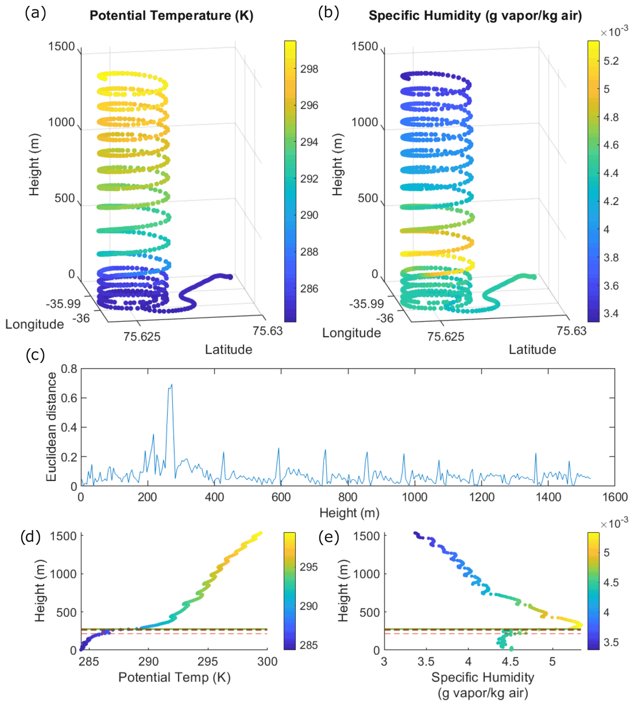
Figure 7 The ascension profile for the 12 June flight mission available to the operator to determine PBL location. The flight path reached a maximum altitude of ∼1500 $\mathrm{m}\mathrm{a}.\mathrm{g}.\mathrm{l}.$ (a and b). The potential candidate for the Euclidean distance determination of the PBL is shown to be at approximately 272.5 $\mathrm{m}\mathrm{a}.\mathrm{g}.\mathrm{l}.$ (c). The top three candidates for PBL all correspond to approximately the same location (green and dotted lines d–e). There is a modest gradient in potential temperature over the flight path of about 16 ^∘K (d). Specific humidity shows an inversion in the first few hundred meters of flight at the determined location of the PBL (e).

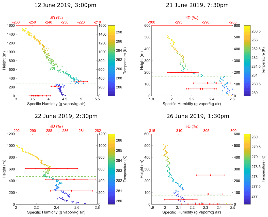
Figure 8 The four flights during the 2019 summer field session at the EastGRIP field camp. Times are presented as local time (UTC − 02:00). Each flight includes a specific humidity and temperature measurement, which is binned for the values at each altitude during the ascension and descent. The result of the determination of the PBL by the operator outlined in Sect. 2.7 is plotted as the dashed green line. The resulting isotope measurements at sampled altitudes are shown in red. Error bars are determined from flask intercomparisons (Sect. 2.6). Additional plots of δ¹⁸O and its relation to δD can be found in Appendix A.

Despite unforeseen challenges, we achieved a total of four sample-taking flights from 12 to 26 June 2019. An example of environmental sensor data for 12 June is shown in Fig. 7. We found varying amounts of structure in isotope space across all four flights (Fig. 8). Large transitions between water vapor isotope surface measurements at 2 m and values above and below the PBL–free-troposphere (FT) transition are apparent in the 12 June flights (Fig. 8). The other flights in contrast had little variability, suggesting that the PBL was unstable (i.e., well mixed). Berkelhammer et al. (2016) suggested that summertime nights at Summit, Greenland, would present the conditions for stable stratification of the atmosphere but that this claim was unprovable using towers alone. In 2022, we will use an improved UAV-system setup to generate a comprehensive diurnal data set spanning many weeks' worth of time.

3.2 Hysteresis and Calinski–Harabasz criterion index (CHCI) and PBL detection

The CHCI was calculated post-flight for comparison with (1) the self-similarity of Euclidean distance (used during the 2019 field campaign but later updated to the CHCI approach) and (2) the operator determination of the PBL. The results are shown in Appendix A. The CHCI had a direct match with Euclidean distance for half of the flights. In the other half, the CHCI predicted altitudes significantly higher than the other determinations. The results of our comparison reveal that our original PBL-detection algorithm using Euclidian distance needs improvement (Fig. 9). Specifically, we have determined that Euclidean distance can under- or overestimate the height of the PBL due to sensor (temperature and humidity) hysteresis. This hysteresis exceeded the stated manufacturer response time for the atmospheric temperatures we encountered, discussed in Appendix B. The hysteresis could be the result either of errors introduced from the changing rate of ascent during flight or from inconsistent airflow over the sensor package resulting from a varying angle of attack of the aircraft (Stickney et al., 1994). Before a flight, the UAV is static at ground level; thus, temperature and humidity measurements will be stable, varying only slightly with small changes in surface conditions. The energetic pneumatically driven launch of the aircraft (a 12 G force) results in a rapid increase in altitude that can introduce a bias into the sensor output due largely to the thermal mass of the sensor and slow response to rapidly changing conditions. A similar effect occurs anytime the rate of ascent is not constant, such as when the UAV transitions between different orbitals (i.e., a sampling orbital and landing orbital).

A case study in Fig. 9 illustrates a shift in orbitals from the 21 June mission. The operator moved from the initial launch orbital to a lower altitude to begin an ascension profile. During the transition between the two orbitals, the aircraft moved from about 110 to 60 m in altitude in ∼1 min. During the transition and immediately during the ascent, multiple temperature and humidity values were generated for the same altitude, creating a region of varying hysteresis effects that can bias PBL prediction by Euclidean distance, ultimately causing the operator to misidentify the altitude of the PBL. More concisely, the algorithm detected this data anomaly as atmospheric structure, when in fact it was due to hysteresis. While removing these skewed data could be an easy fix, the stabilization of temperature and humidity to that new starting altitude biases the beginning of the climb just as it does at the surface before launch.

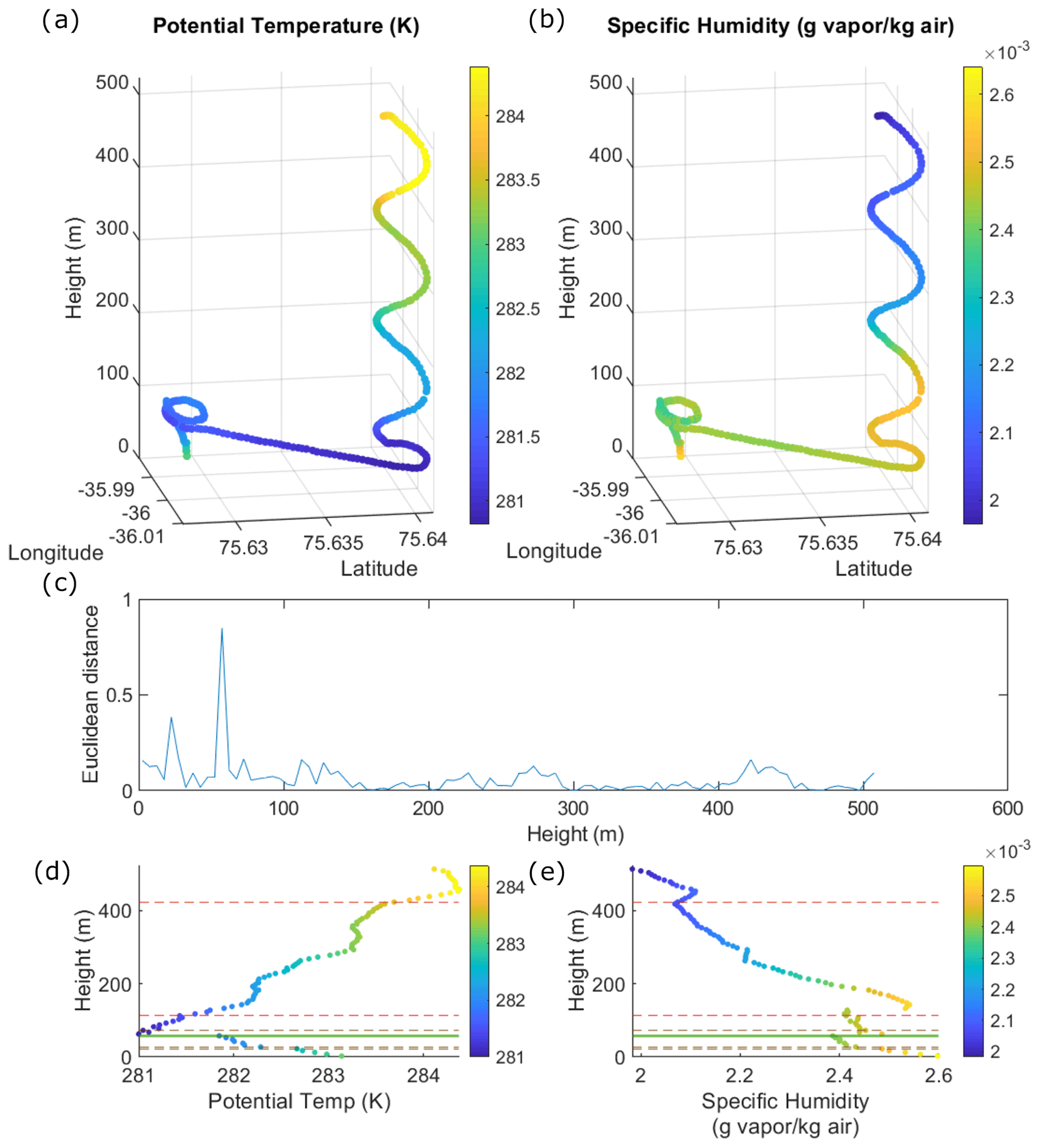
Figure 9 The ascension profile for the 21 June flight mission available to the operator to determine PBL location. The flight reached a maximum altitude of ∼500 m (a and b). Post launch, the operator flew from the initial launch at ∼110 to ∼60 $\mathrm{m}\mathrm{a}.\mathrm{g}.\mathrm{l}.$ over the course of ∼1 min. Settling of both temperature and humidity due to hysteresis during that time was flagged incorrectly by Euclidean distance (c). The resulting predictions of PBL locations (solid green line for the most likely, dashed line for the next four likely, d, e) are scattered across the space.

The hysteresis effect is also noticeable in the CHCI (Fig. 10, green circles). Relaxing the a priori assumption of a single PBL that separates the surface atmosphere from the free troposphere, additional transition regions can be identified. As CHCI uses Euclidean distance to establish variances, it is also subject to potentially poor predictions in situations of significant hysteresis. However, its ability to establish regions of similarity, such as the case of the transition region between launch orbital and the ascension orbital during the 21 June mission, provides an objective method of informing the operator of potential false positives for the boundary layer altitude. In this specific case, three of the top five PBL altitudes predicted by the Euclidean distance algorithm can be flagged as incorrect. However, even with sensor hysteresis, we determine the CHCI to be an effective tool to assist in fast mid-flight evaluation of the boundary layer by the drone operator.

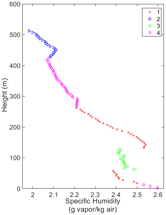
Figure 10 Specific humidity over the ascension for the 21 June flight partitioned into groups by the CHCI with the a priori assumption of K relaxed from 2 to 4. The region of transition the operator took post launch between ∼110 and ∼60 m is clearly evident as a separate group (green circles). In cases where artificial structure exists due to sampling patterns, CHCI may assist the operator by flagging those areas.

Overall, there are two options for overcoming the effects of hysteresis: (1) better sensors and (2) changes to flight mission plans. We have identified the Vaisala RSS-421 sonde sensor to meet the first requirement. The RSS-421 includes a low-thermal-mass fine-wire thermocouple and heated humidity sensor with a bakeout unit, which will allow for faster response in arctic conditions. This sensor has already been shown to be capable of producing accurate temperatures in challenging UAV fixed-wing missions (Frew et al., 2020). For flight planning, relocating launch sites to be as close to the ascension orbital as possible will reduce hysteresis during horizontal transitions between orbitals. The ascension rate can also be slowed to less than 2 m s⁻¹, allowing the maximum time for sensors to equilibrate with the surrounding atmospheric conditions. The tradeoff is that this may require reducing the maximum flight altitude to conserve battery life and reduce the bank angle. A sharp bank angle decreases the lift coefficient (Williamson, 1979), and a higher angle of attack is needed to maintain ascension rate in tailwind situations (Blakelock, 1991). Larger angles of attack could be detrimental as they are known to introduce temperature errors, favoring the use of slower ascension rates (Stickney et al., 1994). Slower ascension rates may be required regardless of when the pitch angle needed is too high, and outside the flight envelope, the Black Swift Technologies autopilot will slow ascension to protect the aircraft. It is assumed that variability in temperature, pressure, and humidity is small in the x and y plane, allowing for a large increase in orbital diameter to reduce bank angle significantly. In future field campaigns, we will test the effect that ascension rate has on hysteresis with the new RSS-421 sonde along with the current sensor, which will remain on the aircraft. We do not expect to eliminate hysteresis entirely, but we do expect to reach precisions appropriate to model PBL–free-troposphere atmospheric isotopic exchange.

4 Conclusions and outlook

We have presented a UAV-isotope sampling platform and methodology capable of measuring atmospheric water vapor and its stable isotopes within the planetary boundary layer (PBL) and lower troposphere in a polar environment. We utilize a fixed-wing UAV (Black Swift Technologies) with flight times in excess of 45 min with the capability to reach 1600 $\mathrm{m}\mathrm{a}.\mathrm{g}.\mathrm{l}.$ Multiple nose cones allow for collection of air in eight glass flasks, enclosed within a 3D-printed support structure that critically withstands 12 G's of force during takeoff. In this study, the total system is used to sample above and below an algorithmically detected PBL, resulting in the first measurements of atmospheric water isotopes above and below the PBL on the high-altitude Greenland Ice Sheet.

Across four sample-taking missions at the EastGRIP ice core site in 2019, we observed significant variation in water isotopes on either side of the PBL; the variability exceeded our conservative precision estimates of 2.8 ‰ in δD and 0.45 ‰ in δ¹⁸O. These results form the basis for future campaigns to collect high-temporal-density measurements (flights every 4–6 h across many weeks) at key missing scales that will improve ice-to-atmosphere modeling and mixing processes, ice sheet mass balance, satellite detection algorithms, moisture tracking, ice core science, and modeling the hydrologic cycle in general.

A field campaign for return to EastGRIP is scheduled for summer 2022. Future improvements to the UAV-isotope system will be primarily focused on logistical improvements that increase the number and frequency of flights. Additional flight crew will be available for nighttime flight missions. To ensure a balanced diurnal flight schedule over weeks of time, with the goal of one flight every 4–6 h, a precessing schedule of calibration times will be used. Each calibration will be done every 2–4 d, lasting 12 h, starting at different times of day. This ensures that we do not consistently lose the ability for UAV sampling at the same time for every calibration, e.g., from 12:00–00:00. The combination of these improvements will allow the potential maximum number of flights per day to increase from two to as many as six, while balancing the timing of calibration. In flight, we will carefully regulate the rate of ascent and include better-performing temperature and humidity sensors with minimal time constants, all of which will reduce hysteresis for PBL detection. We plan to leverage an existing anemometer used by the autopilot in order to assist in the correction as well as produce an additional 2D wind speed for the flight. Additional improvements will include a lighter pump and manifold system that should allow greater flight time. Beyond Greenland, this platform is readily adaptable to other scientific disciplines and will be used in an upcoming permafrost project to measure atmospheric methane emissions and soil moisture content in Alaska.

Appendix A: Additional schematics and figures

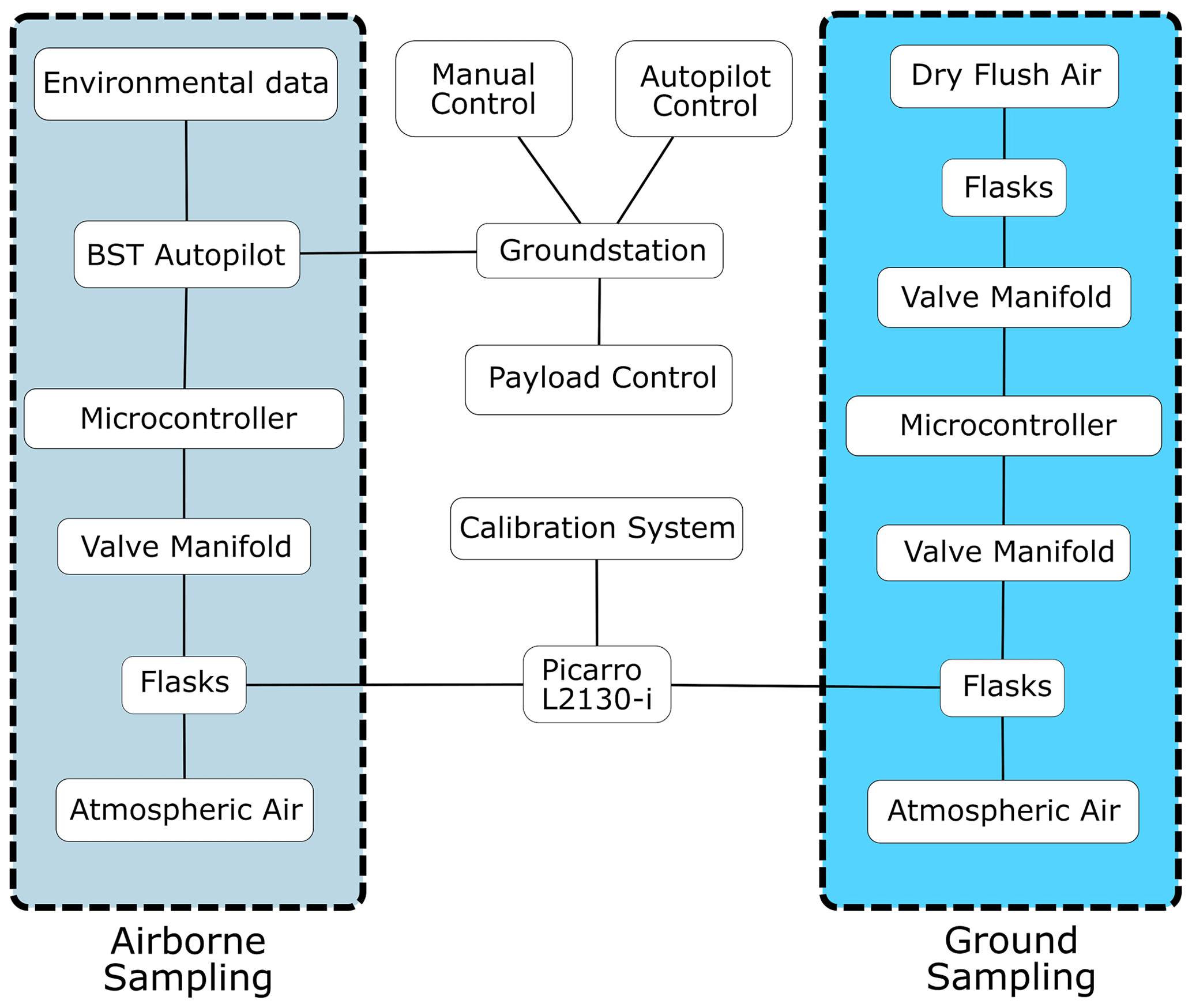
Figure A1 UAV-isotope system diagram showing control and sample exchange between airborne/ground sampling and measurement subsystems. Both ground and airborne sampling are performed identically, though their control methods differ.

Figure A2 Design document for the glass flasks aboard the S2 payload.

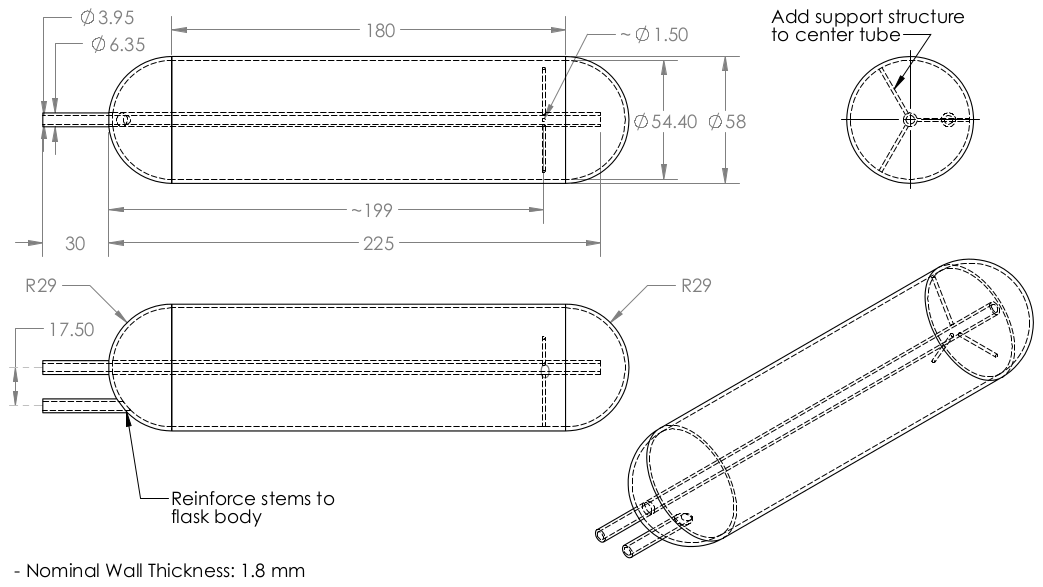
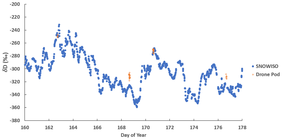
Figure A3 Comparison in δD between the tower setup present at the EastGRIP camp in 2019 and 2 m pod intercomparison measurements. Drone pod measurements on 163 DOY (day of year) and 176 DOY correspond to flask measurements taken at 2 m during a flight mission. All measurements from both tower and UAV are tied to the same isotopic water standards listed in Table 1.

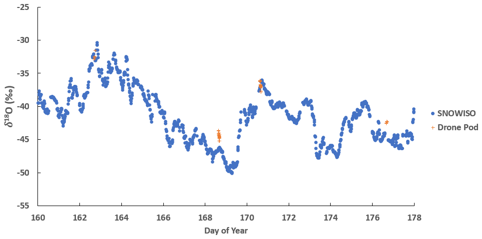
Figure A4 Comparison in δ¹⁸O between the tower setup present at the EastGRIP camp in 2019 and 2 m pod intercomparison measurements. Drone pod measurements on 163 DOY (day of year) and 176 DOY correspond to flask measurements taken at 2 m during a flight mission. All measurements from both tower and UAV are tied to the same isotopic water standards listed in Table 1.

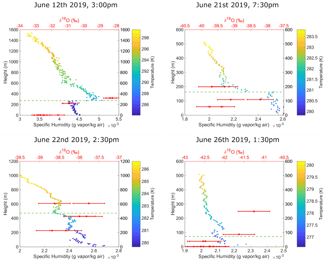
Figure A5 The four flights during the 2019 summer field session at the EastGRIP field camp. Includes collected environmental data during flight for both ascent and descent as well as measured isotope values for oxygen.

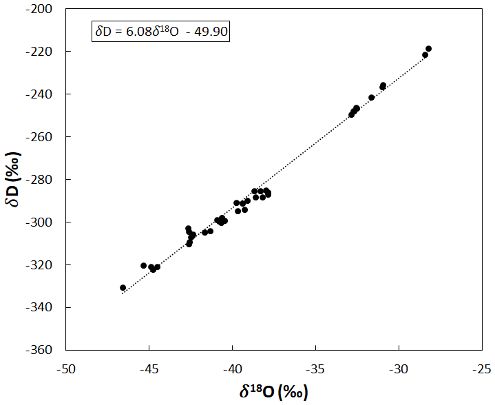
Figure A6 Relation plot between δD and δ¹⁸O for all four flights as well as pod intercomparison tests taken at 2 m.

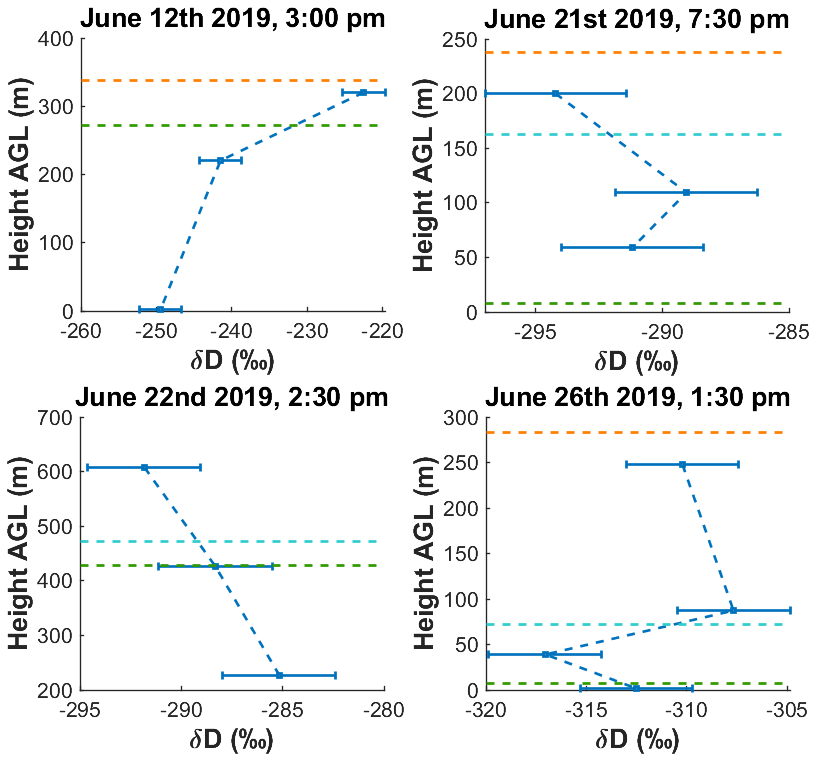
Figure A7 A comparison between different methods of determining the location of the PBL. The location predicted from the first off-diagonal of Euclidean distance is indicated by the green dashed line. When the CHCI prediction is different, it is plotted in orange. When the operator determined a different location of the PBL, it is plotted in cyan. To illustrate the structure observed relative to these predictions, average isotopic values of δD for flasks taken at each height are shown in blue.

Appendix B: Hysteresis correction

A supplier-listed hysteresis curve was used to correct for the capacitive humidity sensor (HC103M2) aboard the ee03 sensor used on the Black Swift Technologies S2. Note that observed hysteresis was much greater than this.

Table B1 Empirically determined response times for the HC103M2 humidity sensor at different temperatures provided by the supplier.

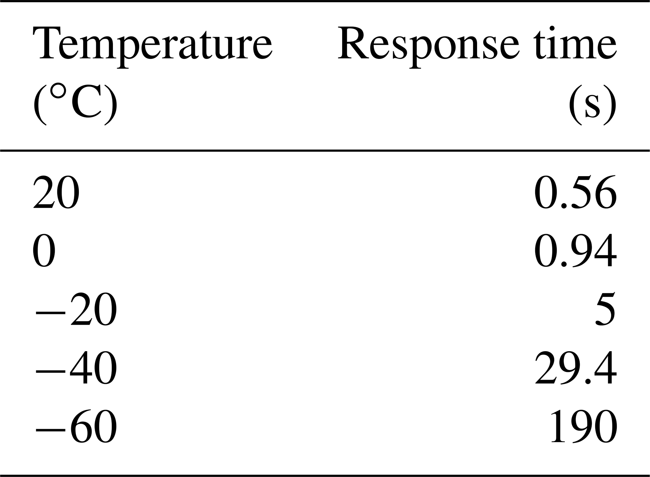
The correction was made by linearly interpolating a function (MATLAB fit() function) with the above values to determine measured time vs. true time and then applied to the altitude that represents the new time for the measurement. https://www.epluse.com/fileadmin/data/product/hc103m2/datasheet_HC103M2.pdf (last access: October 2020).

A supplier-listed response time for temperature measurement of the ee03 sensor was not available within the temperature ranges measured within the study and assumed to be negligible.

Appendix C: The S2 drone

Scientific missions the S2 has flown prior to this study include mapping soil moisture with a radiometer (Dai et al., 2017 ), a calibration mission including a 12-band multispectral camera system (Wang et al., 2016), measuring snow-water equivalent with a radiometer (Yueh et al., 2018), and a volcano sampling mission that involves difficult operations into the plume of an active volcano (Wardell et al., 2017). The S2 is currently in use by the National Oceanic and Atmospheric Administration (NOAA) for wildfire applications (Gao et al., 2018), and it has flown in various challenging environments, including at high altitude during atmospheric sampling campaigns in the San Luis Valley in Colorado (de Boer et al., 2018). The S2 is designed for operations at altitudes up to 6000 $\mathrm{m}\mathrm{a}.\mathrm{m}.\mathrm{s}.\mathrm{l}.$ in support of the National Aeronautics and Space Administration (NASA) science missions (Elston and Stachura, 2018).

The S2 utilizes the SwiftCore™ Flight Management System for avionics control, communication, and command, designed by BST. It comprises the SwiftPilot™, SwiftStation™, and SwiftTab™ user interface, along with support electronics. SwiftTab™ runs on Android devices like smartphones or tablets. Flight plans (1) can be uploaded, created, and modified before and during flight; (2) can use georeferenced data points for systematic surveying, including pre-defined banking and spirals; and (3) are fully autonomous from launch to landing. Immediate preliminary analysis and decision-making is supported via real-time telemetry and control capabilities.

Table C1 Black Swift Technologies S2™ specifications.

Appendix D: Euclidean distance and the Calinski–Harabasz criterion index

To compare clusters, a distance needs to be established. The abstract length of a vector in a real vector space is the L^p-norm (Eq. D1), defined as distance d_p between two points a and b with m features, where p is any real number and p≥0.

$$\begin{array}{}\text{(D1)}& {\displaystyle }\begin{array}{rl}{d}_p[a,b]=& \left(\right|b_{\mathrm{1}}-a_{\mathrm{1}}{|}^p+|b_{\mathrm{2}}-a_{\mathrm{2}}{|}^p+\mathrm{\cdots }+\\ & |b_m-a_m{|}^p{)}^{\mathrm{1}/p}\end{array}\end{array}$$

The Euclidean distance (L²-norm) between specific humidity and potential temperature was chosen to be an effective distance (Toledo et al., 2014). In a self-similarity plot of pairwise distance between all points, the maximal distance between points, represented as the first off diagonal, provides a predictive tool for PBL height (Fig. 7). In the clustering analysis, environmental measurements were averaged into 5 m vertical bins and normalized between 0 and 1.

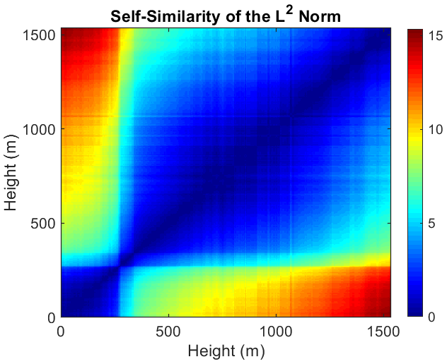
Figure D1 Plot of the self-similarity matrix of the L²-norm of atmospheric values determined for the sampling flight on 12 June 2019. The first off diagonal represents the comparison of every value against every other value. This method was used to identify the PBL during all 2019 flight operations, later updated with the Calinski–Harabasz criterion index.

While Euclidean distance is more robust than individual gradient analysis (Krawiec-Thayer, 2018), the technique still returns multiple candidates for the PBL height. Instead, indexing methods can provide a deterministic global maximum of centroid partitions associated with the data set. For the Calinski–Harabasz criterion index, the centroid is determined with a nonhierarchical k-means method. k-means is a data-partitioning algorithm that determines groupings of k amount of centroid clusters of n total observations converging to a maximum criterion value or index between centroids. k is determined a priori to be 2, corresponding to the assumed present atmospheric regions, the PBL and free troposphere. The Calinski–Harabasz criterion index has been used successfully with k-means methods in previous remote sensing and weather balloon studies (Toledo et al., 2014; Caicedo et al., 2017).

The Calinski–Harabasz index is the ratio of variance within one centroid and the variance between origin locations of all other centroids. Let m_i be the centroid of cluster i containing n_i data points and c be an origin point for the data set. The variance within one cluster is defined below in Eq. (D2):

$$\begin{array}{}\text{(D2)}& {\displaystyle }{\displaystyle }{D}_W=\sum _{x\mathit{ϵ}\mathit{\alpha }}\left(d_{\mathrm{2}}\right[x,m_a]{)}^{\mathrm{2}}+\sum _{x\mathit{ϵ}\mathit{\beta }}(d_{\mathrm{2}}[x,m_{\mathit{\beta }}]{)}^{\mathrm{2}}.\end{array}$$

The expression for variance between clusters is defined as

$$\begin{array}{}\text{(D3)}& {\displaystyle }{\displaystyle }{D}_B=n_{\mathit{\alpha }}\left(d_{\mathrm{2}}\right[m_a,c]{)}^{\mathrm{2}}+n_{\mathit{\beta }}(d_{\mathrm{2}}[m_{\mathit{\beta }},c]{)}^{\mathrm{2}}.\end{array}$$

The ratio of variances, the Calinski–Harabasz index, then follows as

$$\begin{array}{}\text{(D4)}& {\displaystyle }{\displaystyle }\text{CH}=(n_{\mathit{\alpha }}+n_{\mathit{\beta }}-\mathrm{2})D_B{D}_W^{-\mathrm{1}}.\end{array}$$

The centroid pair with the highest index is then the most significant group of partitions, and the height that corresponds with the boundary of the two groups is assumed to be the upper layer of the PBL. An example of this method is shown in Figs. 6 and 10.