the Creative Commons Attribution 4.0 License.
the Creative Commons Attribution 4.0 License.
 | 17 Nov 2021
Correction of wind bias for the lidar on board Aeolus using telescope temperatures
Fabian Weiler
Michael Rennie
Thomas Kanitz
Lars Isaksen
Elena Checa
Jos de Kloe
Ngozi Okunde
Oliver Reitebuch
The European Space Agency (ESA) Earth Explorer satellite Aeolus provides continuous profiles of the horizontal line-of-sight wind component globally from space. It was successfully launched in August 2018 with the goal to improve numerical weather prediction (NWP). Aeolus data have already been successfully assimilated into several NWP models and have already helped to significantly improve the quality of weather forecasts. To achieve this major milestone the identification and correction of several systematic error sources were necessary. One of them is related to small fluctuations of the temperatures across the 1.5 m diameter primary mirror of the telescope which cause varying wind biases along the orbit of up to 8 m s−1. This paper presents a detailed overview of the influence of the telescope temperature variations on the Aeolus wind products and describes the approach to correct for this systematic error source in the operational near-real-time (NRT) processing. It was shown that the telescope temperature variations along the orbit are due to changes in the top-of-atmosphere reflected shortwave and outgoing longwave radiation of the Earth and the related response of the telescope's thermal control system. To correct for this effect ECMWF model-equivalent winds are used as a reference to describe the wind bias in a multiple linear regression model as a function of various temperature sensors located on the primary telescope mirror. This correction scheme has been in operational use at ECMWF since April 2020 and is capable of reducing a large part of the telescope-induced wind bias. In cases where the influence of the temperature variations is particularly strong it was shown that the bias correction can improve the orbital bias variation by up to 53 %. Moreover, it was demonstrated that the approach of using ECMWF model-equivalent winds is justified by the fact that the global bias of model u-component winds with respect to radiosondes is smaller than 0.3 m s−1. Furthermore, this paper presents the alternative of using Aeolus ground return winds which serve as a zero-wind reference in the multiple linear regression model. The results show that the approach based on ground return winds only performs 10.8 % worse than the ECMWF model-based approach and thus has a good potential for future applications for upcoming reprocessing campaigns or even in the NRT processing of Aeolus wind products.
- Article
(3561 KB) - Full-text XML
- BibTeX
- EndNote


The European Space Agency (ESA) Earth Explorer satellite Aeolus was successfully launched into space in August 2018 with an intended mission lifetime of 3 years (Kanitz et al., 2019; Reitebuch et al., 2020). Aeolus, built by Airbus, is equipped with the first-ever functioning space-borne Doppler wind lidar (DWL) instrument ALADIN (Atmospheric LAser Doppler INstrument) and provides globally distributed vertically resolved wind measurements from the ground up to 30 km (ESA, 1999; Reitebuch, 2012a). It measures the component of the wind vector along the instrument's line of sight by emitting ultraviolet (UV) laser pulses into the atmosphere and detecting the frequency-shifted backscatter signal from molecules and particles (ESA, 2008). The main goal of Aeolus is to improve numerical weather prediction (NWP) by filling gaps for global wind measurements in the Global Observation System of the World Meteorological Organization (WMO), especially in the tropics and the Southern Hemisphere (Andersson, 2018; Stoffelen et al., 2005, 2020). Another goal is to improve our understanding of the atmospheric dynamics, especially in the tropics. As spin-off data products, Aeolus provides continuous information about aerosol and cloud distribution, including vertical profiles of backscatter and extinction coefficients (Ansmann et al., 2007; Flamant et al., 2008).
The operational assimilation of Aeolus observations into the European Centre for Medium-Range Weather Forecasts (ECMWF) NWP system was started (Rennie and Isaksen, 2020) on 9 January 2020, followed by other weather centers around the world, such as the German weather service DWD (Deutscher Wetterdienst), Météo-France and the UK Met Office. A prerequisite for this major milestone was the quick identification and correction of the two most important systematic error sources of the Aeolus wind measurements (Reitebuch et al., 2020; Rennie, 2018). The first one was linked to dark current anomalies, so-called “hot pixels”, on the Aeolus detectors which cause systematic wind errors of up to several meters per second. This issue was successfully mitigated on 14 June 2019 by applying appropriate correction methods based on dedicated dark signal calibration measurements (Weiler et al., 2021). The second one, independent of the hot pixel issue, was linked to unexpectedly large systematic errors which strongly vary with geolocation. Thanks to the collaborative effort of the teams within the Aeolus Data Innovation and Science Cluster (DISC) (Reitebuch et al., 2019) and the first discovery at ECMWF (Rennie and Isaksen, 2020), a strong correlation of the wind bias with temperature variations across the primary mirror of the telescope could be identified as the root cause of the latter issue.
The small primary mirror temperature variations of 0.3 ∘C, which are related to varying outgoing top-of-atmosphere (TOA) radiation and corresponding response of the primary mirror's thermal control (TC) to that, lead to varying wind errors along the orbit of up to 8 m s−1. Thermal changes in the instrument's components along the orbit were already expected before launch. However, it was assumed that these variations would be of smaller error magnitude and would be mainly of a harmonic orbit-related nature (Reitebuch et al., 2018b). As the telescope-induced bias turned out to be strongly scene-dependent and not perfectly harmonic, bias correction tools, which were developed before the Aeolus launch, could not be applied to the discovered complexity. As a consequence, a new bias correction method using the temperatures of the Aeolus telescope from the Aeolus housekeeping telemetry as independent variables was developed and has been successfully implemented into the operational near-real-time (NRT) processing chain of Aeolus since 20 April 2020.
This article aims to provide a detailed overview of the influence of the telescope temperature variations on the Aeolus winds and the method to correct for the telescope temperature-induced wind bias. Section 2 of the paper briefly describes the measurement principles of Aeolus, the design and thermal control of the telescope, and the Aeolus wind data products. Section 3 depicts the telescope-induced wind bias and explains the bias correction method in detail. Section 4 demonstrates the performance of the wind bias correction scheme based on a case study with special settings for the telescope temperatures and also shows the reliability of the method when applied to the complete observation period of 6 months using Aeolus data from the first data reprocessing campaign from June to December 2019. The paper concludes with a summary and an outlook for further analysis.
This section gives an overview of the measurement principle of ALADIN followed by a description of the instrument's telescope and its thermal control. Finally, the Aeolus data products and variables necessary for this study are presented. For more detailed information about the instrument, please refer to ESA (2008), Reitebuch et al. (2018a), Reitebuch (2012a), or Lux et al. (2021).
2.1 ALADIN configuration and measurement principle
Aeolus flies in a sun-synchronous dusk/dawn orbit at a mean altitude of 320 km with a repeat cycle of 7 d. The satellite carries one single payload, the direct-detection Doppler wind lidar which is pointing toward the Earth under a 35∘ off-nadir angle towards the dark side of the terminator, the line separating the sunlit from the nighttime areas (Reitebuch, 2012a). The instrument consists of three main components, the laser transmitter, the telescope and the receiver unit. The ultra-violet laser transmitter emits nanosecond pulses with a pulse repetition frequency of 50.5 Hz and an energy of ∼ 60 mJ into the atmosphere (Lux et al., 2020a) where the light is scattered on air molecules, aerosols and cloud particles (Reitebuch, 2012b). The backscattered light from the atmosphere is collected by a Cassegrain-type telescope which consists of two mirrors. The primary mirror collects the light and the secondary mirror reflects it through a hole in the primary mirror to the receiver unit where the Doppler frequency shift of the backscatter light is analyzed. The receiver combines a Fizeau interferometer (FIZ) to analyze the narrow spectral bandwidth backscatter signal from aerosols and cloud particles (Mie channel) and two sequential Fabry–Pérot interferometers (FPIs) (Rayleigh channel) to measure the broad bandwidth backscatter signal from molecules. The Mie channel uses the fringe-imaging technique which is based on measuring the wind-speed-dependent horizontal displacement of interference patterns (McKay, 1998). The Rayleigh channel incorporates the double-edge technique which uses two FPIs as spectral filters that are symmetrically placed around the transmitted laser wavelength (Chanin et al., 1989; Flesia and Korb, 1999; Garnier and Chanin, 1992). In the presence of a Doppler frequency shift the Rayleigh spectrum is shifted towards the spectral peak transmission of one of the two filters. Thus, from the contrast between the transmission of two filters the wind speed along the line of sight of the instrument can be determined. Afterwards, a projection to the horizontal plane, the so-called horizonal line of sight (HLOS), is obtained.
For both channels accumulation charged-coupled devices (ACCDs) are used to image the output of the spectrometers (ESA, 2008; Weiler et al., 2021). In the 16×16 pixel illuminated imaging area the return signal is integrated over time based on the vertical range gate settings. The integration time is adjustable and can be changed from 2.1 to 16.8 µs which corresponds to vertical sampling of 250 to 2000 m, considering the 35∘ off-nadir angle of the instrument. Afterwards, the signals of each range gate are binned together and are continuously shifted downwards to the non-illuminated memory zone of the ACCD which consists of 16×16 pixels in which each row corresponds to one range gate. In the memory zone the return signals of 18 consecutive laser pulses are accumulated to so-called measurements with a duration of 0.4 s (∼ 2.9 km horizontal resolution). Afterwards, the accumulated charges are digitized with 16-bit accuracy and converted into numbers of least significant bits (LSBs). In the on-ground processing the signal of typically 30 measurements is accumulated to so-called observations with a duration of 12 s which corresponds to a spatial horizontal resolution of 86.4 km (see Fig. 1) for a satellite ground track speed of 7.34 km s−1.
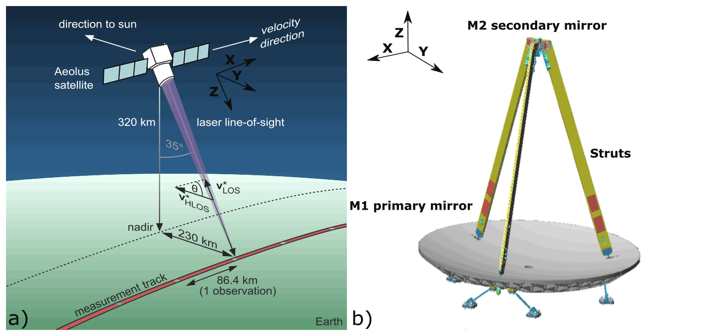
Figure 1(a) Aeolus observational geometry (adapted from Lux et al., 2020b) and (b) the setup of the Aeolus telescope consisting of the M1 primary and M2 secondary mirrors and the mounting struts (adapted from https://directory.eoportal.org/web/eoportal/satellite-missions/a/aeolus, last access: 23 August 2021).
2.2 Aeolus telescope
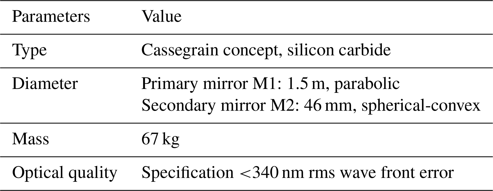
Aeolus is operated in a mono-axial transceiver configuration which means that the same telescope is used to transmit and receive the light. The Cassegrain telescope consists of a parabolic 1.5 m diameter primary “M1” mirror and a convex, spherical 46 mm diameter secondary “M2” mirror attached to three mounting struts (see Fig. 1). The main components of the telescope are made of silicon carbide (SiC).The wave front error, defined as the deviation of the telescope's wave front from the perfect spherical, was determined after the instrument assembly to be below 150 nm rms (root mean square) which is within the specification of 340 nm rms (Korhonen et al., 2008). The distance between the M1 and M2 mirrors is 1.32 m. The main specifications of the Aeolus telescope are summarized in Table 1. A baffle around the complete telescope structure is used to shield the secondary mirror and the mounting struts from direct sun illumination. On the sun-remote side of the satellite the baffle is shortened to reduce mass and air drag. As Aeolus is facing different thermal conditions on its orbit which influence the thermal stability of the M1 mirror, an active thermal control system is used. The thermal control of the M1 mirror aims to keep the temperature of the M1 mirror stable at a fixed temperature setpoint of 12 ∘C throughout the orbit, using thermal control (TC) thermistors located on the back side of the mirror. For additional temperature monitoring further temperature sensors also located on the back side of the mirror, the so-called accurate housekeeping thermistors (AHTs), are available. The AHT sensors are not used in the active thermal control system of the telescope. Measurements of both sensor types are provided for each observation every 12 s in the Aeolus data products. The location of the sensors on the M1 mirror is indicated in Fig. 2. The sensors TC-23, TC-29 and TC-32 which are mounted on the bottom and lateral shields of the mirror are not indicated in the figure and are not used in the thermal control loop of the telescope.
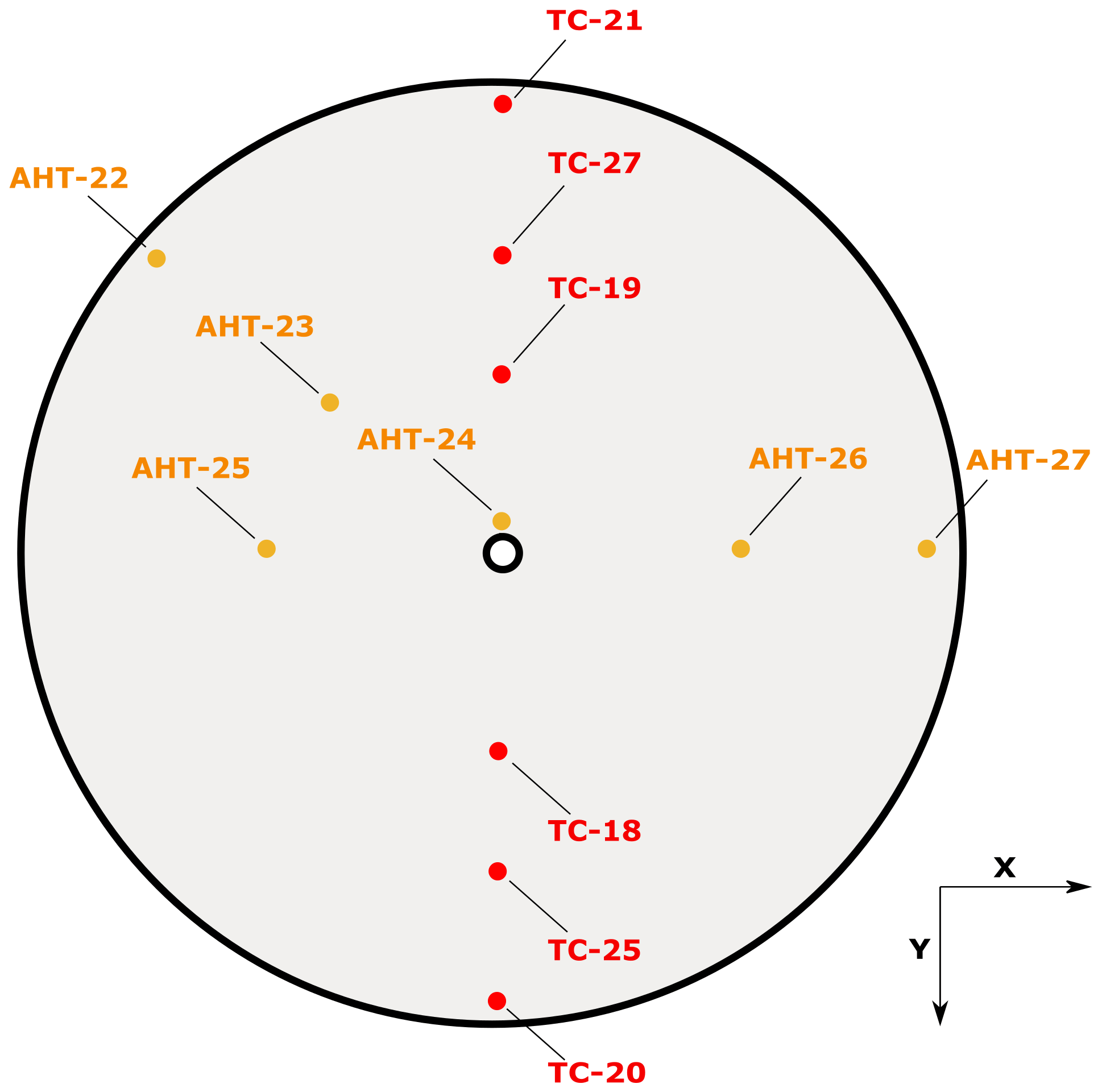
Figure 2A schematic illustration of the Aeolus M1 mirror. The red and orange dots indicate the positions of the thermal control (TC) and accurate housekeeping (AHT) thermistors. X indicates the flight direction. Note that TC-23, TC-29 and TC-32 are not shown.
To control the focus of the telescope the thermal control of the struts and the M2 mirror can be adjusted using dedicated heaters. This allows us to change the distance between the M1 and the M2 mirrors which affects the focus of the telescope. So-called instrument telescope refocus (ITR) measurements are carried out on a regular basis to determine the best focus with respect to the radiometric performance of the instrument and using the spot width on the Rayleigh channel ACCD as a measure for the telescope's focus. During these measurements, the temperature setpoints of the strut's and M2 control thermistors are varied in the range between 6 to 16 ∘C in order to derive the optimum setpoint with the best focus.
2.3 Aeolus data products
The Aeolus data processing which is managed by ESA's Payload Data Ground Segment (PDGS) includes several stages to process the raw detector counts up to the main wind product, namely the Level 2B (L2B) data product which contains the fully processed horizontal line-of-sight (HLOS) winds for the Mie and Rayleigh channels (Straume, 2018; Rennie et al., 2020). To continuously improve the quality of the Aeolus data products for use of Aeolus products in operations at NWP centers, the operational processors are usually updated twice a year. Updates for auxiliary files which are used to control certain settings of the processors do not follow a fixed schedule and are updated more often. The term “baseline” is part of the PDGS administration and is used to describe a collection of products that have been produced in a similar way, i.e., using processor versions with similar major version numbers and mostly unchanged algorithm settings.
2.3.1 Level 1B
In the L0 and L1A steps, the housekeeping information which consists of various satellite and instrument parameters (e.g., temperatures, pressure, currents, etc.) is processed, and the raw signal data are geo-referenced. The L1B processor provides processed ground echo data and preliminary winds which are not corrected for atmospheric temperature and pressure influences (Reitebuch et al., 2018a) at the so-called observation level which corresponds to a temporal resolution of 12 s corresponding to a spatial horizontal resolution of 86.4 km (see Fig. 1). Within the various processing steps, the L1B processor uses a ground detection scheme to flag return signals as ground return signals (Weiler, 2017) with the aim to use these ground detections for zero-wind calibration (ZWC). Solid ground is assumed to be a non-moving object and thus can be used as a zero-wind speed reference. In addition, this also allows possible ground-affected range bins to be flagged since mixing ground and atmospheric backscatter in the same range bin will lead to incorrect wind retrievals. In a first step, the L1B ground detection algorithm identifies ground bin candidates based on a signal-gradient threshold approach (Weiler, 2017). Next, several checks are performed to further restrict the selection of ground bins. For instance, the distance of the ground bin candidates to a model of the Earth's surface is evaluated, and the signal intensity of the ground bin candidates is also assessed to identify valid ground bins. In a final step, the wind retrieval is applied to the valid ground bin signals to retrieve the ZWC winds (Reitebuch et al., 2018a). The ZWC winds are contained for each channel at observation level in the L1B products and can be used as reference for the M1 bias correction (see Sect. 3.3). The sensitivity of the ground detection algorithm can be controlled by several parameters. For the presented work reprocessed Aeolus L1B data products, processed using the same processor versions as for baseline 1B11 but with custom ground detection settings, from June to December 2019 were used. For these data products quite relaxed parameter settings for the ground detection were used. The minimum ground useful signal thresholds were set to zero for both channels, which leads to a high number of ground returns in the L1B product. Since also the ground return signal is reported in the L1B product, it is possible to use the ground useful signal as quality criterion by applying a minimum threshold. In the framework of this analysis, a minimum useful signal threshold of 9700 LSBs is applied to the Rayleigh ZWC winds, making sure that gross outliers are removed from the dataset.
2.3.2 Level 2B
The L2B processing (Tan et al., 2008) includes a correction of the Rayleigh winds for temperature and pressure broadening effects (Dabas et al., 2008). This correction is based on a priori temperature and pressure information from short-range forecasts from the ECMWF weather forecast model. Moreover, the measurement signals (∼ 2.9 km horizontal resolution) from the Mie and Rayleigh channels are classified according to their optical properties based on the scattering ratio and signal-to-noise ratio (SNR) derived from the Mie channel. This allows for the classification of measurements into so-called “clear” (molecular backscatter) and “cloudy” (particulate backscatter) results to avoid contamination from spectrally narrow bandwidth Mie signals in the Rayleigh channel, which would result in errors in the retrieved wind speed (when not accounted for). The classified measurements are then grouped together and horizontally accumulated to optimize the signal-to-noise ratio. The accumulation length is variable and depends on the processor settings and the characteristics of the measurement signals. Due to the different SNR characteristics of the Mie and Rayleigh signals, the accumulation length is also different for both channels. For the Mie channel, the signals are typically accumulated over a horizontal scale of at most ∼ 10 km, whereas the accumulation length for the Rayleigh (clear air) signals is at most ∼ 86 km. It should be noted that for mixed scenes containing both clear and cloudy sections, the accumulation length may be smaller, and this may differ for different altitudes. Afterwards, the wind retrieval is separately applied to each accumulated signal portion to yield two HLOS so-called “wind results” for each channel: Rayleigh clear and cloudy; and Mie clear and cloudy. In general, the focus lies on the Rayleigh clear and Mie cloudy wind results since they are of better quality. It should be noted that the Mie clear wind results are physically not meaningful and are a result of the classification process. As part of the wind retrieval, a cross-talk correction is applied to the Rayleigh wind results to further minimize Mie contamination (Rennie et al., 2020). Moreover, the L2B products also contain quality flags and wind error estimates for each wind result.
For the presented work Aeolus L2B data products produced by the PDGS, labeled with baseline 2B10, from June to December 2019 were used.
2.4 ECMWF model and O−B statistics
For monitoring purposes, equivalent HLOS winds from the ECMWF model are calculated for each L2B wind result. For this, information from the Aeolus auxiliary meteorological files (AUX_MET) which amongst many variables contains wind vector information along the predicted Aeolus track is used (Rennie et al., 2020). The information in the AUX_MET file is updated every 12 h and is based on short-range forecasts obtained from the operational ECMWF high-resolution model TCO1279 (∼ 9 km grid spacing, cubic-octahedral spectral transform with spectral truncation of n=1279) (Malardel et al., 2016) with a maximum forecast range of up to 30 h. The information in the AUX_MET files is provided every 3 s along the orbit at 137 model levels interpolated (nearest neighbor) to the Aeolus track. To compute observation minus background (O−B) statistics, the L2B processor uses a nearest-neighbor approach in the horizontal and uses the closest profile in the AUX_MET file in the selected time window. In the vertical dimension a spline interpolation is used to get a value at the proper altitude. The O−B statistics have been used to analyze the systematic and random wind errors of the Aeolus observations at a global scale (Martin et al., 2021). The term “background” refers to the background model forecast which serves as a priori information for the next analysis run in the data assimilation (Rennie and Isaksen, 2020). From 20 April 2020 (as implemented in L2BP v.3.30, starting with Level 2B products labeled baseline 09) onwards, O−B statistics also have been added to the operational Aeolus L2B products. The first reprocessed dataset from June to December 2019 also includes this improvement.
For the following analysis of the dependency of the wind bias on the M1 temperatures, a representative average O−B value “E(O−B)” is calculated from the L2B O−B values. For this only L2B wind results with the overall validity flag set to “true” are used. In addition, HLOS error estimates, reported for each L2B wind result, are used as quality criterion. Only Mie and Rayleigh wind results with HLOS error estimates smaller than 4 and 8 m s−1, respectively, are considered. As mentioned above, the O−B values are available for each L2B wind result. However, to decrease the variance of the bias, the O−B values are horizontally averaged to the L1B observation granularity (12 s temporal and 86.4 km horizontal resolution). For long wind result accumulation lengths, the L1B observation might be covered by only one single wind result. In such cases, no averaging is performed. Afterwards, the O−B values are averaged over all range gates to yield the E(O−B) value. This is justified by the lack of altitude dependency of the M1 bias effect as the measured M1 temperatures are constant over all altitudes. Figure 3 shows the typical distribution of the center-of-gravity altitudes of the L2B Mie cloudy and Rayleigh clear wind results. This plot indicates that for the Mie channel a large fraction of wind results in the lower altitudes contribute to the E(O−B) statistics. In contrast, the Rayleigh wind results show a broad distribution with an equal contribution of the wind results in the altitude range between 5000 and 18 000 m. As explained in the following sections, the E(O−B) value is used to derive the fit coefficients for the M1 bias correction. Thus, the information from Fig. 3 should be kept in mind when analyzing the altitude dependency of the error of M1 bias-corrected L2B wind results.
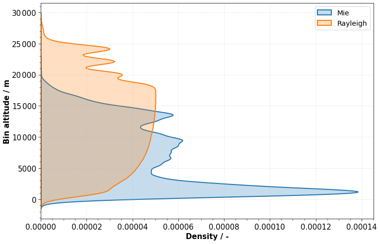
Figure 3Density curves of the center-of-gravity altitudes of the Mie cloudy (blue) and Rayleigh clear (orange) L2B wind results. A total of 74 202 Mie and 132 042 Rayleigh wind results obtained from 8 August 2019 were used to derive the probability density curves. Only valid wind results with HLOS error estimates smaller than 4 and 8 m s−1 for the Mie and Rayleigh channels, respectively, are shown.
It is obvious that the use of the NWP model for the bias correction introduces some NWP model bias dependency since the ECMWF model wind biases are not zero. However, this is justified by the fact that on average the global bias of the model wind u components with respect to reference measurements based on radiosondes is relatively small. This is demonstrated in Fig. 4, which shows the time series of daily averages of E(O−B) values of the ECMWF's u-component winds computed for radiosondes and pilots (radiosondes that only measure wind). It should be mentioned that the comparison is restricted to locations where radiosondes and pilots are available, which is mainly above the Northern Hemisphere land surface. Thus, it is difficult to accurately assess the model bias in the Southern Hemisphere or above oceans. Nevertheless, Fig. 4 shows that during all days the bias is clearly below 0.3 m s−1, which is significantly smaller than the Aeolus M1-related bias (for the Rayleigh), justifying the choice of the ECMWF model as a reference for the bias correction. To mitigate the influence of model wind bias, 24 h of global model winds averaged over all altitudes are used in the M1 bias correction. On the one hand, this makes sure that localized small-scale model biases (e.g., in the tropics) appear only as a noise source in the fit procedure. On the other hand, averaging over all altitudes ensures that any altitude-varying model bias is not an issue.
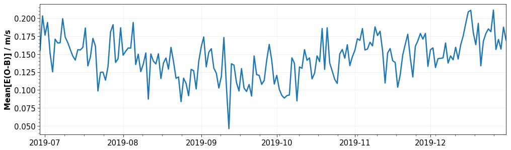
Figure 4Time series of global (at all available radiosonde and pilot locations) 24 h averages of E(O−B) values of ECMWF's u-component winds computed for radiosondes and pilots (radiosondes that only measure wind) at all model levels.
The following section describes the correlation between the wind bias and the M1 telescope temperatures. Moreover, the approach to remove the M1-dependent bias using O−B values and ZWC winds as a bias reference is explained, and its limitations are discussed.
3.1 Telescope-induced wind bias
Before launch, harmonic (with respect to the orbit phase) bias contributors, induced by thermal effects and pointing variations of the attitude control system that mainly depend on the latitudinal position of the satellite and the orbit phase, were expected to be dominant. These kinds of error contributors were supposed to be corrected with the so-called harmonic bias estimator (Reitebuch et al., 2018b). This tool was set up before launch based on end-to-end simulations of the assumed harmonic errors using ZWC winds as a reference to correct for harmonic bias variations. However, it turned out that this kind of correction was far from being sufficient to correct the bias variation as seen in Aeolus in-orbit data despite the wind biases having some harmonic behavior.
Figure 5 shows in-orbit measurements of the Rayleigh clear E(O−B) values as a function of the orbit phase angle (argument of latitude) on 11 August (blue) and 11 November (orange) 2019. The argument of latitude describes the position of the satellite and is defined as 0∘ at the ascending node Equator crossing and 360∘ at the descending node Equator crossing. For both cases the bias shows complex and non-perfectly harmonic dependencies with the orbit phase. Moreover, it was found that the bias structure changes over the seasons and is strongly dependent on the atmospheric scene, i.e., cloudiness and the TOA temperature. Comparing both cases in Fig. 5 shows smaller bias amplitudes in the Southern Hemisphere in November than in August. On top of that, the bias shows strong longitudinal dependencies, i.e., non-harmonic elements, which are indicated by the large spread of the bias at a fixed orbit phase, e.g., at around 45∘ argument of latitude for the August case.
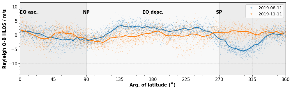
Figure 5Rayleigh clear E(O−B) HLOS statistics as a function of the argument of latitude on 11 August (blue) and 11 November (orange) 2019. The argument of latitude describes the position of the satellite along its orbit in the ascending (asc., dark grey) and descending (desc., light grey) orbit phase (EQ: Equator; NP: North Pole; SP: South Pole). The blue and orange dots indicate the E(O−B) values which correspond to averaged O−B values over all altitudes at observation level (introduced in Sect. 2.4). The blue and the orange lines show the E(O−B) values as binned averages using a bin size of 5∘ for the argument of latitude.
Bell et al. (2008) found strong correlations between housekeeping temperature data and biases for the Special Sensor Microwave Imager/Sounder (SSMI/S) mission, so easy access to housekeeping data for Aeolus was requested early on during the design of the ground segment. The comparison of the O−B statistics with available housekeeping data then revealed a high correlation of the Rayleigh bias with the M1 temperatures. In particular, a strong linear correlation was found between the Rayleigh bias and the radial temperature gradients of the M1 telescope mirror. This relationship was first discovered at ECMWF and is described in more detail in Rennie and Isaksen (2020). The radial temperature gradient can be described by the following combination of the sensors located at the outer and inner parts of the telescope (see Fig. 2): (mean(AHT_27, TC_20, TC_21) – mean(AHT_24, AHT_25, AHT_26, TC_18, TC_19)). Thus, negative values for the radial temperature gradient indicate a warmer central part of the telescope and vice versa.
Further investigations have shown that the orbital variations in the radial temperature gradient are linked to changes in TOA radiation. Figure 6 shows the relationship between the radial temperature gradient measured by Aeolus and the outgoing longwave radiation (OLR) obtained from the NOAA Climate Data Record (CDR) of daily OLR. This dataset is derived from observations from imagers on board several geostationary satellites such as the High-resolution Infrared Radiation Sounder (HIRS) instrument on board the NOAA19 satellite, and it provides daily averages of global OLR measurements (Lee and NOAA CDR Program, 2011). OLR measurements from 1 October 2019 were collocated with Aeolus measurements from the same day and averaged along the Aeolus orbit for 60 observations (720 s) resulting in 1388 collocations. It has to be noted that the relationship was found to be not perfectly linear (depicted by the red line in Fig. 6), and for other days the nonlinearity seems to be stronger. But due to the response of the thermal control of the telescope to the changing environment and the fact that shortwave radiation is not considered in the regression analysis, no perfectly linear relation is expected. However, the results depicted in Fig. 6 clearly demonstrate the correlation between TOA OLR and changes in the radial temperature gradient of the M1 telescope and motivated further studies of the wind bias correlation with the radial temperature gradient.
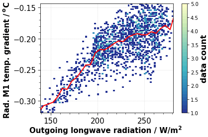
Figure 6Correlation between the radial M1 mirror temperature gradient and the daily-averaged TOA outgoing longwave radiation measured by the HIRS instrument on board several NOAA satellites on 1 October 2019 (Lee and NOAA CDR Program, 2011). The red line shows the radial M1 temperature gradient as a function of the outgoing longwave radiation as binned averages (5 W m−2 bin size).
To illustrate the relationship between the Rayleigh bias and the mirror temperatures Hovmöller diagrams are generated. Hovmöller diagrams allow us to analyze temporal as well as spatial characteristics of a quantity at the same time. Typically, time is plotted on the x axis, and the spatial variable, in this case the latitude of the observation, is used as the y axis. In the Hovmöller diagrams of Fig. 7, the mean over all M1 temperature sensors (top), the radial temperature gradients (middle) and the Rayleigh clear E(O−B) values (bottom) are shown at observation level for the complete observation period. It shows that the mean M1 temperature values vary quite remarkably with geolocation and time in the range between 12.9 and 14.5 ∘C. The observed patterns suggest that the variations are due to the changes in the TOA short- and longwave radiation of the Earth and the response of the thermal control to that. The mean M1 temperatures show a quadrupole-like structure which is visible for ascending as well as descending orbits. Minimum values appear in Northern Hemisphere summer (June to July) and winter (November to February) in the region of the North Pole and South Pole, respectively. Two dominant maximum regions occur in the Southern Hemisphere between July and November and in the Northern Hemisphere between September and January. During polar summer in both hemispheres the high outgoing shortwave radiation fluxes in the polar regions heat up the M1 mirror. This is then compensated for by the thermal control system which explains the colder mean M1 temperature values in these regions for these periods. In a similar way the positive anomalies during Northern Hemisphere and Southern Hemisphere winter can be explained. Here, the reduced reflected solar radiation cools down the M1 mirror which is compensated for by actively heating up the M1 mirror. It is remarkable that the intertropical convergence zone (ITCZ) which is characterized by low longwave outgoing radiation is visible in the M1 temperatures. When the satellite passes by the ITCZ, the thermal control reacts by heating the mirror which increases the mean M1 temperatures after the ITCZ. Comparing the mean M1 temperatures between ascending and descending orbits indicates a slight phase shift of the structures between both phases. This can be explained by the inertia of the thermistors and the reaction of the thermal control system. When the satellite crosses the relatively cold ITCZ it takes some time for the thermal control to respond. As a result, the ITCZ appears slightly shifted to the north and south for ascending and descending orbits, respectively.
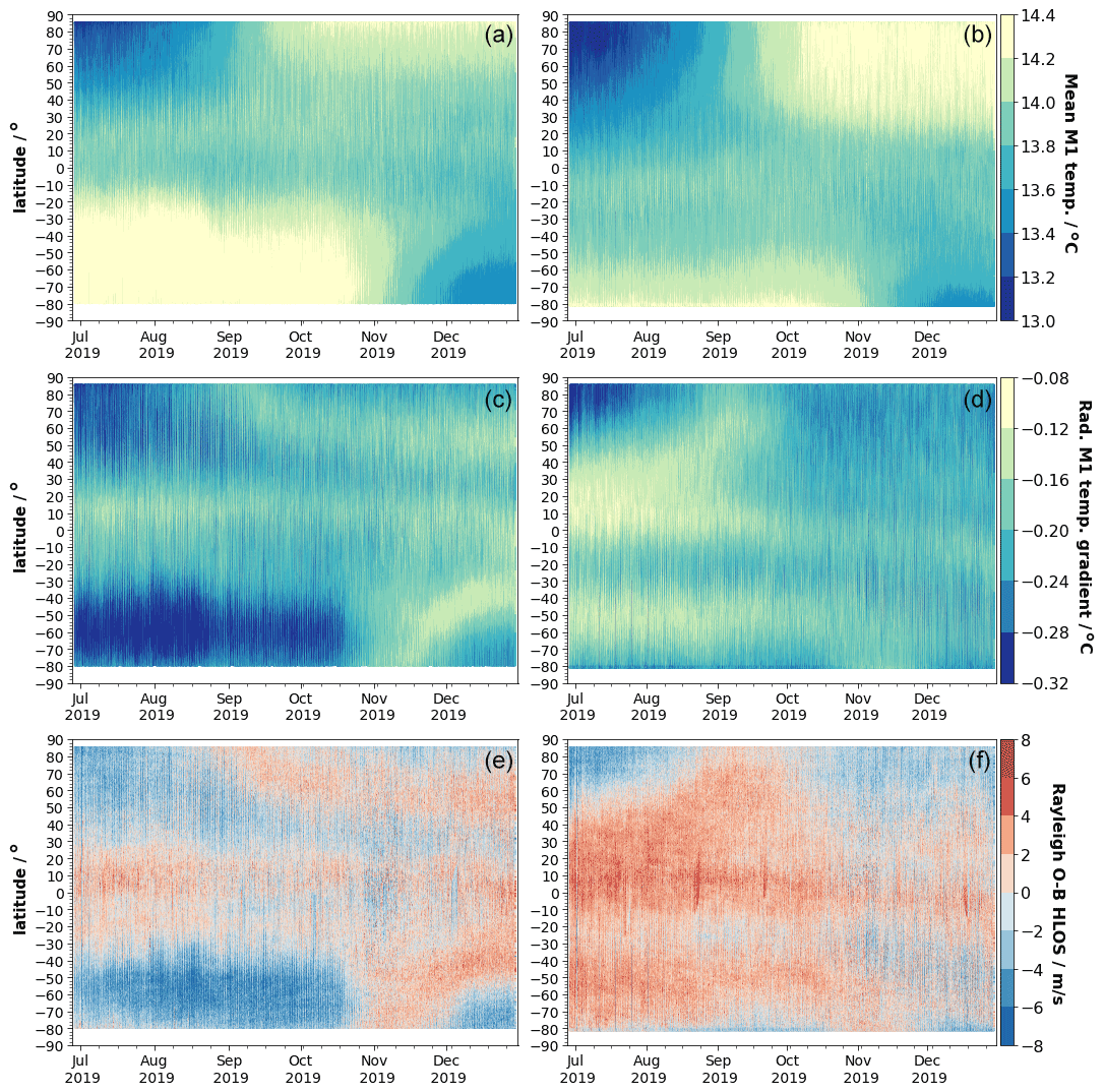
Figure 7Hovmöller diagrams of the average over all M1 temperatures (a, b), the radial temperature gradient of the M1 telescope (c, d) and the Rayleigh clear E(O−B) HLOS values (e, f) from 28 June to 31 December 2019 split up into ascending (a, c, e) and descending (b, d, f) orbit phases.
The middle panel of Fig. 7 shows the radial temperature gradients (as introduced above) along the M1 mirror. Knowing that the central part of the mirror is more exposed to radiation changes, many of the features can be explained such as the difference of the radial gradients between ascending and descending orbits around the South Pole during Southern Hemisphere winter. Here, the satellite crosses the very cold areas of the Southern Hemisphere polar vortex which makes the central part of the mirror relatively cold (red colors). Afterwards, on the ascending orbit phase the thermal control responds by heating the central part, which results in relatively warmer inner telescope temperatures (blue colors). Comparing the radial temperature gradients (middle) with the Rayleigh clear E(O−B) values (bottom) demonstrates the strong correlation between the bias and the M1 radial temperature gradients. Note that sometimes the bias is due to other issues than changes in the M1 temperatures. For instance, the striking bias anomalies close to the Equator for descending paths around mid-August or mid-September are related to the star tracker of the spacecraft being blinded by the moon leading to an incorrect determination of the satellite-induced LOS velocity and thus systematic wind errors.
The radial temperature changes in the M1 mirror along the orbit which are up to 0.4 ∘C most likely affect the shape of the mirror. This would change the focus of the telescope and other higher order aberrations, and hence, it causes slightly different angular illumination patterns (e.g., incidence angle and divergence) of the light passing through the field stop and illuminating both spectrometers. Both spectrometers are sensitive towards angular changes in the incoming light and thus produce an apparent frequency shift which manifests as wind bias. Further analysis also shows that the radiometric performance of the instrument is affected by the thermal variations in the telescope (Flament et al., 2021).
It should be noted that also sensitivity of the Mie bias to the M1 temperatures was thoroughly investigated. The sensitivity was found to be ∼ 10 times less than for the Rayleigh channel. This could be explained by the fact that the beam for the Mie spectrometer is increased by a beam expander in front of the Mie spectrometer by a factor of 1.8, thus reducing the divergence of the light. Furthermore, the Rayleigh spectrometer is specifically sensitive to the incidence angle variation because of its sequential implementation of the two Fabry–Pérot interferometers (Reitebuch, 2012b). Hence, the focus of the analysis below is on the correction of the Rayleigh wind bias.
3.2 Bias correction using the ECMWF model
The discovery of the strong linear correlation between the radial gradients of the M1 telescope temperatures (Rennie et al., 2021) and the wind bias paved the way towards the development of an operational bias correction scheme. For this, a multiple linear regression (MLR) approach choosing all available thermistors as independent variables is used to describe the E(O−B) values as a function of the following 15 M1 temperatures: AHT-22, AHT-23, AHT-24, AHT-25, AHT-26, AHT-27, TC-18, TC-19, TC-20, TC-21, TC-23, TC-25, TC-27, TC-29 and TC-32 (Fig. 2). A prerequisite for the operational correction was the adaption of the L1B and L2B processors to include these variables in the operational data products (since baseline 2B09), which was a huge achievement by the DISC team given the short amount of time for preparation. With this information the MLR model can be defined as follows:
where β0 is the intercept, β1⋯β15 are the coefficients for each temperature variable, and ε denotes the error term. In terms of reducing the bias, it turned out that the MLR showed better mathematical performance than a linear model that is based on the radial physical temperature gradient of the telescope (see Sect. 3.1; Rennie and Isaksen, 2020).
Figure 8 demonstrates that the MLR model described in Eq. (1) is a suitable choice for this task. For the diagnosis, in the same way as is done for the NRT processing, past data, in this case from 11 August 2019, are used to predict the bias on 12 August 2019. Note that for the reprocessing data from the same time period are used to derive the fit coefficients. The big advantage for reprocessing is the availability of the complete dataset which makes it possible to apply the MLR model to the same time period that was used to train the model. This even further improves the performance of the bias correction scheme as no predictions with unseen data have to be performed. The left scatter plot indicates the high correspondence between the model prediction and the measured bias values. This is demonstrated by the high R2 value of 0.78. The right panel of Fig. 8 is generally used to indicate if the model residuals show remaining patterns that are not fully captured by the model (James et al., 2014). This is done by plotting the model residuals against the predicted values. In our case, the residuals are equally scattered around zero without dominant patterns justifying the MLR approach. There seems to be a slight hint for remaining residual bias (<0.3 m s−1) in the range between 0 to 2 m s−1. This is shown by the smooth curve fitted using weighted least squares (red line) fit to the residuals which shows slightly negative values in this region.
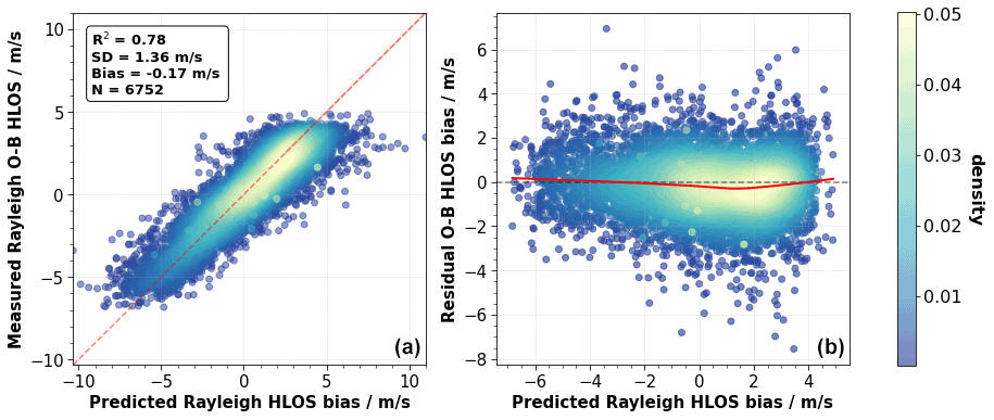
Figure 8Diagnostic plots for the multiple linear regression with the measured Rayleigh clear E(O−B) values (a) and the model residual (b) as a function of the predicted bias (a). Data from 11 August 2019 are used to predict the bias on 12 August 2019. The red line in (a) indicates the diagonal. In the text box of (a) values for the coefficient of determination (R2 ), standard deviation (SD) ]and the bias of the corrected values, as well as the number of data points (N) used in the regression, are shown. The red line in (b) indicates the smooth function obtained after applying locally weighted smoothing. The color coding in both panels indicates the kernel density.
Figure 9 demonstrates the application of the M1 bias correction for 12 August 2019. For this example, the model fit coefficients β0,⋯β15 are derived from Rayleigh clear E(O−B) values from 11 August 2019 and are used to predict the Rayleigh clear E(O−B) values on the next day. The panels compare corrected (orange) with uncorrected (blue) E(O−B) values as a function of time (Fig. 9a) and the argument of latitude (Fig. 9b). To measure the performance of the bias correction approach to decrease the bias variation along the orbit, the standard deviation of the E(O−B) values, i.e., SD(E(O−B)), can be used. In the case depicted in Fig. 9, this value is reduced by 52.8 % from 2.89 to 1.36 m s−1 (also see the text box in Fig. 8), which clearly demonstrates how well this method works to reduce most of the M1-induced bias variation along the orbit. The remaining residual variation of 1.36 m s−1 is considered to be of a random nature arising from instrumental and forecast model random errors, and it does not contain any obvious regular patterns. It should be noted that this value of the standard deviation is representative for altitude averages of the E(O−B) value at L1B observation granularity, in contrast to the wind random error which is defined as the standard deviation of each single observation within a vertical profile.
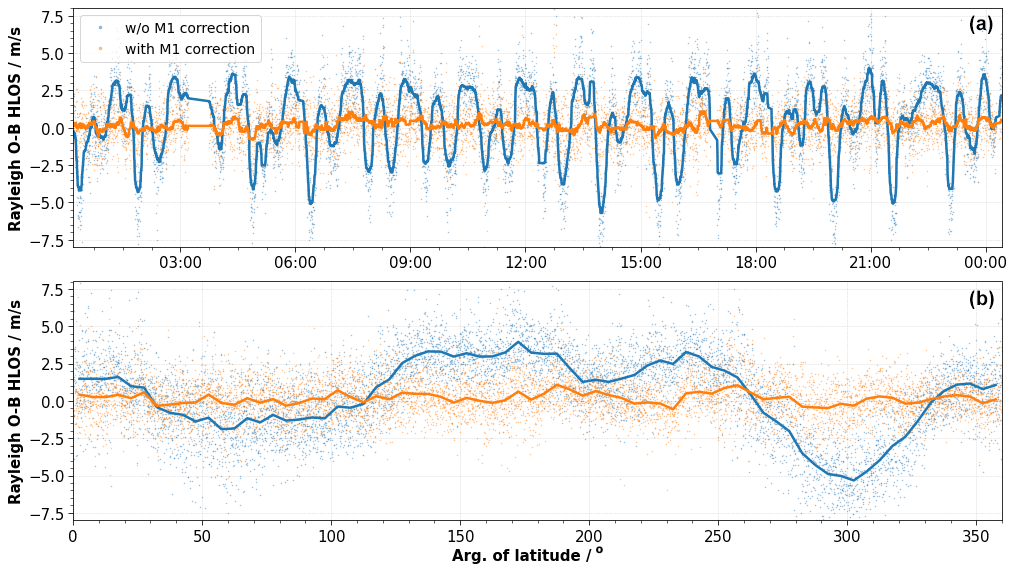
Figure 9Rayleigh clear E(O−B) HLOS values as a function of time (a) and the argument of latitude (b) during 12 August 2019. The blue and the orange dots indicate the bias without and with M1 bias correction, respectively. The blue and the orange lines show temporal (5 min interval) and binned (5∘ bin size for the argument of latitude) averages of the E(O−B) values, respectively. The M1 bias correction coefficients are derived from data from 11 August 2019.
For the M1 bias correction in the operational processing chain, dedicated software was developed which was put into operation on 20 April 2019 (starting with Level 2B products labeled baseline 09). Figure 10 depicts the flow chart of the M1 bias correction for the Aeolus NRT operational processing chain. The AUX_TEL software uses 24 h of past L2B data as input, performs the MLR (see Eq. 1) and writes the model coefficients β0⋯β15 into an auxiliary telescope (AUX_TEL_12) file. The generation of the AUX_TEL_12 file is updated every 12 h. The AUX_TEL_12 file is used as input by the L2B processor for the M1 bias correction of the wind results. This is done by solving Eq. (1) using measured M1 temperatures and the derived model fit coefficients to yield an M1 bias correction value for each L2B wind result of both channels. As a next step, the bias correction values are subtracted from the measured wind results and provided in the L2B products as bias-corrected winds. Note that bias correction values are also written into the Earth Explorer format L2B product, which allows users to undo the M1 bias correction.
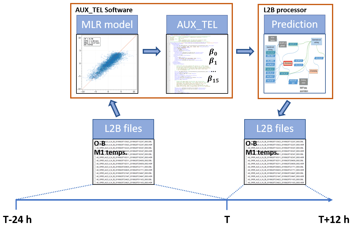
Figure 10Flow chart of the operational M1 bias correction of the L2B wind results. In the AUX_TEL software, 24 h of past L2B data with the E(O−B)-values as dependent and the 15 M1 temperatures as independent variables are used as input for the multiple linear regression (MLR) model. The model software produces an AUX_TEL file which contains the model coefficients β0⋯ β15. Afterwards, the L2B processor uses the AUX_TEL files to make a prediction for the wind bias and to correct the wind results of the subsequent 12 h window. Then, the AUX_TEL file is updated in the same way.
The high update frequency of 12 h for the AUX_TEL_12 generation is necessary because the model parameters β0⋯β15 are slowly changing with time, which indicates that the sensitivity of the instrument towards telescope temperature variations is changing over time. Moreover, this allows us to capture the slowly drifting global average bias. Investigations have shown that the global average bias changes are due to a slow drift of illumination of the Rayleigh spectrometers in the internal path (particularly for the second laser, the Flight Model (FM)-B laser). In order to capture this effect, it was decided to implement an intercept term, β0 (see Eq. 1), into the model which makes sure that the mean of the model residuals, i.e., the mean [E(O−B)] value of the analyzed period, is zero. To avoid large constant bias offsets from the model, the mean winds are anchored to the ECMWF model twice per day, and the AUX_TEL_12 generation is updated every 12 h. The introduced bias offset depends on the change rate of the internal reference response in the 12 h interval. For the analyzed period, the maximum change (worst case) was considerably small at 0.78 m s−1. To make sure that the sample size is large enough and the fit coefficients are derived with a sufficiently high enough accuracy, 24 h of past data (∼ 6500 samples) are used in the MLR.
As mentioned before, the Mie cloudy winds are much less affected by thermal variations in the M1 mirror. However, it was decided to also use the same correction approach for the Mie winds mainly for the reason to correct for global bias offsets of the Mie cloudy winds, again related to internal path drifts.
3.3 Bias correction using ground return winds
The operational M1 bias correction procedure makes use of ECMWF model winds and thus introduces some dependency on the NWP model. But as mentioned in Sect. 2.4, this is justified by the low model wind bias with respect to radiosondes (see Fig. 4). In addition, the M1 bias correction uses 24 h of global model winds averaged over all altitudes, which is why small-scale model biases (e.g., in the tropics) appear only as an additional noise source in the fit procedure. Moreover, altitude-dependent ECMWF model bias is not an issue as vertically averaged E(O−B) statistics are used in the MLR model.
However, to overcome this issue of model dependency, it is also possible to use Aeolus' L1B ground return winds (see Sect. 2.3) as a reference instead of E(O−B) values. Ground return winds can be seen as a zero-wind reference to correct for systematic wind error sources such as the M1 temperature-induced wind bias. However, the use of ground return winds as reference is hampered by the limited spatial and temporal coverage of ground returns. The availability of ground returns with high enough ground signals is mainly restricted to polar regions with high surface albedo. The top panel of Fig. 11, which displays Rayleigh clear O−B HLOS and ZWC winds before the application of the M1 correction as a function of the argument of latitude during 11 August 2019, shows the large difference of the data availability between O−B and ZWC values. In this case, the availability of winds is mainly restricted to the ice-covered regions around Antarctica, which results in a rather small sample size of 659 ZWC winds compared to 6897 O−B values. However, it turned out that the coverage of ZWC winds is sufficiently high, i.e., enough different O−B values are covered, to use ZWC winds as a bias reference in the M1 bias correction. The plot shows a large correspondence between O−B and ZWC values as both indicate the same M1-dependent bias structure. Note that the constant offset of about 3 m s−1 between O−B and ZWC values is due to the different calibration procedure between L1B and L2B winds and is quite consistent with time (Dabas et al., 2008; Reitebuch et al., 2018a; Rennie et al., 2020). It is not considered to be a problem for the bias correction since this offset could be corrected in the data processing.
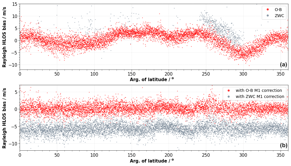
Figure 11(a) Rayleigh clear O−B HLOS values (red) and Rayleigh ZWC HLOS winds (grey) without M1 correction as a function of the argument of latitude during 12 August 2019. (b) The red and grey points indicate the Rayleigh clear O−B HLOS values after the M1 correction using O−B values and ZWC values as a bias reference, respectively. The M1 bias correction coefficients for both approaches (ZWC, O−B) are derived from data from 11 August 2019.
In contrast to the MLR model defined in Eq. (1) a slightly different approach is used to describe the ZWC winds as a function of the M1 temperatures. Due to the lower sample size a simplified model with fewer independent variables has to be used. In the case that the sample size is small compared to the number of model coefficients, overfitting can occur, meaning that the model tends to describe the noise rather than the physical relationship in the data. In such a case, the capability of the model performing predictions with unseen data is drastically reduced. To avoid this issue, different MLR model combinations were tested, and for each combination the skill in predicting the bias was evaluated. It was found that a grouping of the thermistors into two groups which describe the temperature at the outer and inner parts of the M1 mirror provides the best results: G1 = mean(AHT27, TC20, TC21) and G2 = mean(AHT24, AHT25, AHT26, TC18, TC19). The bias correction model is then described as follows:
where α0 is the intercept, α1 and α2 are the coefficients for each temperature group G1 and G2, and ε denotes the error term. For the M1 bias correction of L2B winds Eq. (2) is solved using measured M1 temperatures and the derived model coefficients α1 and α2 to yield an M1 bias correction value for each L2B wind result. The bottom panel of Fig. 11 shows the application of the ZWC-based M1 correction for 12 August 2019. The grey curve indicates the Rayleigh clear O−B HLOS values after the ZWC-based M1 correction. To compare both approaches, the O−B bias after the ZWC-based M1 correction (grey) is shown together with the operational O−B-based bias correction (red). This demonstrates that also the ZWC-based approach is capable of reducing most of the M1 temperature-induced bias variation. The ZWC approach reduces the SD(E(O−B)) from 2.89 to 1.40 m s−1, which is only slightly worse than the O−B-based approach achieving a reduction to 1.36 m s−1. The offset between both curves is a result of the different calibration procedure between L1B and L2B winds as discussed above. The similar performance of the ZWC approach also helps us to confirm that the O−B approach is doing the correct thing and not introducing too many ECMWF model bias-related artifacts.
In this section, it is demonstrated that the M1 bias correction also works with different temperature set point conditions for the thermal control thermistors of the primary telescope mirror (see Sect. 2.2). Moreover, the performance of the M1 bias correction using O−B values is evaluated for the completed observation period from 28 June to 31 December 2019, demonstrating the reliability of this method. In addition, the performance of the bias correction using ground return winds is shown.
4.1 Case study
In order to decrease the orbital variation in the wind bias and increase the atmospheric return signal, in-orbit tests were carried out to optimize the thermal control of the telescope from 6 to 10 July 2020. The main goal of the tests was to decrease the orbital variations in the M1 mirror radial thermal gradients by modifying the control law coefficients of the heater lines. The thermal control of the M1 mirror is based on a proportional integration differential (PID) control loop which controls the heating power applied to the TC sensors. The control law coefficients can be used to optimize the response of the control loop. Figure 12a shows the evolution of the radial M1 temperatures (see Sect. 3.1) before and during the M1 optimization tests. The radial gradients are shifted towards higher values, and the range is also increased from −0.3 to −0.1 ∘C before the test to −0.25 to 0.1 ∘C during the test. As a result, the Rayleigh clear bias (blue line in bottom panel of Fig. 12) also changed significantly. The panel indicates a decrease in the variability in the bias on sub-orbital timescales but an increase in the bias variability on longer timescales. However, the orange line that indicates the M1-corrected bias clearly demonstrates the capability of the M1 bias correction approach to also perform well with new temperature settings. In this case, data from the same day are used to derive the fit coefficients. During the optimization test the M1 bias correction improved the standard deviation of the O−B values by 53.2 % from 5.09 to 2.70 m s−1. This example also shows how the M1 bias correction removes the global offset introduced by changes in the illumination in the internal path (see Sect. 3.2). In this case, the offset improves on average from −7.49 to 0.0 m s−1.
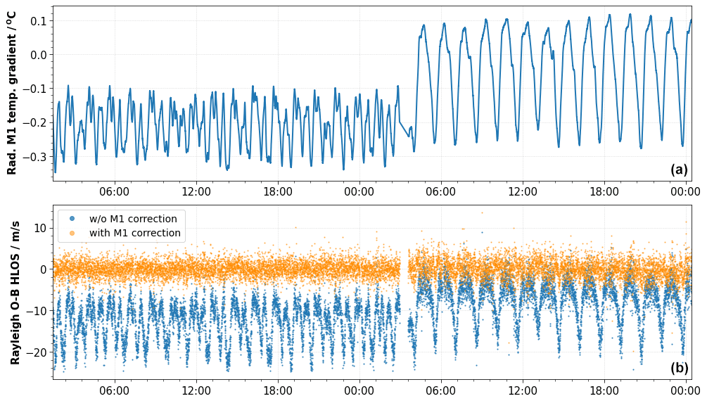
Figure 12The radial temperature gradient of the M1 telescope (a) and the Rayleigh clear E(O−B) HLOS values (b) as a function of time during the M1 optimization tests on 5 and 6 July 2020. The blue and the orange dots indicate the bias without and with M1 bias correction, respectively. Data from day N are used to predict the bias on day N. The periodicity (especially visible in the second half of the plot) is related to the orbital phase of the satellite which is ∼ 91 m.
This important finding implies that the M1 telescope-induced bias can be handled by ground processing in all circumstances, and further M1 optimization tests can now be fully focused on optimizing the radiometric performance of the instrument.
4.2 Performance time series
Figure 13 shows the performance of the M1 bias correction for the period from 28 June to 31 December 2019. To generate the time series, data from day N were used to predict the wind bias on day N+1. The top panel shows daily averages of the standard deviation of the Rayleigh values SD(E(O−B)) before and after the application of the M1 correction based on O−B and ZWC values. In general, this panel shows a changing seasonal influence of the M1 temperature-induced Rayleigh bias. At the beginning of the period from July to October the largest variability in the radial gradients of the M1 temperatures along the orbit can be observed (see Fig. 7), which leads to large M1 temperature-induced wind bias and hence a large improvement by both bias correction approaches. For instance, on 15 July 2019 M1 bias correction drastically reduces the SD(E(O−B)) values from 2.29 to 1.24 and 1.37 m s−1 for the O−B and ZWC approaches, respectively. For the following period between August and October a steady decrease in the M1 influence on the Rayleigh wind bias can be seen. This is mostly related to a seasonal effect that decreases the orbital variability in the radial temperature gradients on the descending orbit phase (see Fig. 7). In October and November, the M1 temperature-induced bias variability reaches its minimum. During this period, the influence of the bias correction on the Rayleigh wind bias is very small. The plateau of increased standard deviation values between 28 October and 15 November is during a campaign period with a special range gate setting with smaller range gates to achieve finer altitude resolution around the tropopause, resulting in higher random wind errors. Afterwards, the seasonal effect on the M1 temperature variations slowly starts to increase again.
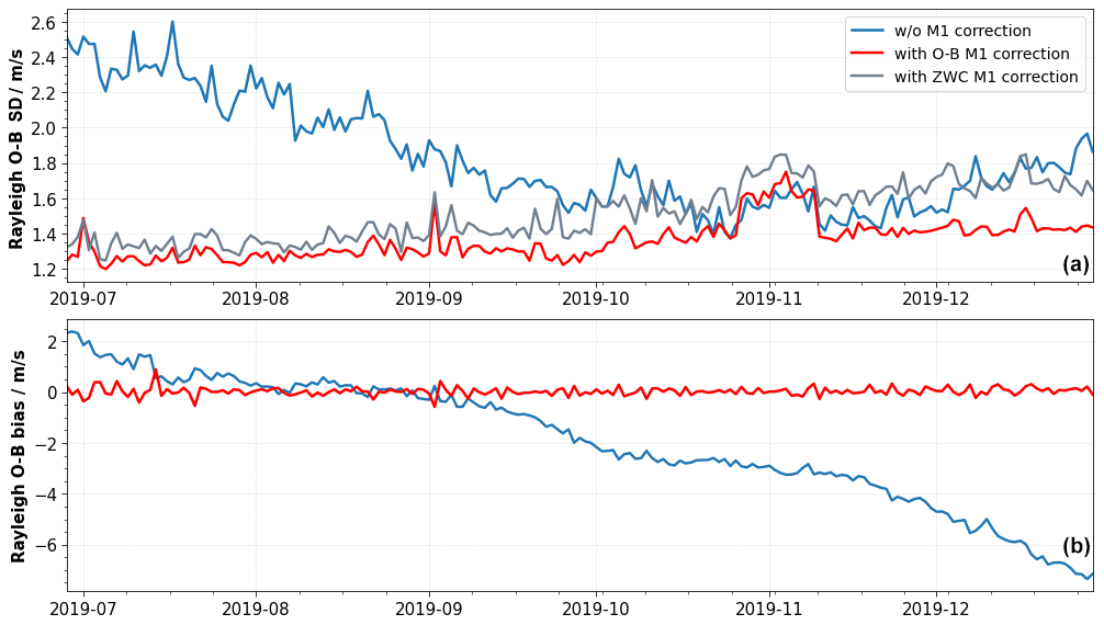
Figure 13Performance of the O−B (red) and ZWC M1 bias correction (grey) methods for the period from 28 June to 31 December 2019. (a) Time series of daily averages (15 orbits) of the standard deviation (SD) of the Rayleigh clear E(O−B) HLOS values before (blue) and after the O−B- and ZWC-based M1 correction (red and grey, respectively). (b) Daily averages of the bias of the Rayleigh clear E(O−B) HLOS values before (blue) and after the O−B-based M1 bias correction (red). Data from day N are used to predict the bias on day N+1.
The difference between the performance of the O−B (red) and ZWC (grey) approaches is not constant. On average, the ZWC approach is 10.8 % worse than the O−B-based correction with a maximum deviation of up to 25.6 %. However, one should bear in mind that the verification against O−B itself will naturally favor the O−B method. Especially at the end of period, when the M1 influence on the wind bias is low, the performance of the ZWC approach decreases and is not able to further improve the SD(E(O−B)) values. As a consequence, it was decided to use the ECMWF model as reference for the operational correction of the NRT products. However, methods to further improve the performance of the ZWC-based approach are still under investigation, which might allow us to use this approach for future reprocessing or even NRT processing of the Aeolus data products, removing the need for ECMWF model winds as a reference. Other NWP centers have confirmed the low biases with respect to their own independent NWP models following the operational implementation of the M1 temperature bias correction, which is reassuring.
It is worth noting that the M1 bias-corrected SD(E(O−B)) values show a steady increase of 11.3 % from 1.24 m s−1 at the beginning to 1.40 m s−1 (O−B based) at the end of the period. This is due to a combination of decreasing laser emitted energy from 65 to 61 mJ and a loss of the optical signal throughput in the receive path of the instrument. Without the implementation of the accurate M1 bias correction, it would not have been possible to observe the increase in the random error based on wind error statistics as the M1 effect dominates the SD(E(O−B)) values. The daily averages of the uncorrected SD(E(O−B)) values (blue curve in the top panel of Fig. 13) show a decrease from the beginning of the period until October 2019, related to the changing seasonal influence of the M1 temperature-induced bias. This decrease could be misinterpreted as a decrease in the random wind error. Only after correcting for the M1 effect is the true random error evolution revealed.
The bottom panel of Fig. 13 shows the temporal evolution of daily averages of the Rayleigh clear mean(E(O−B)) values with (red) and without (blue) O−B-based M1 correction. As mentioned in Sec. 3.2, the M1 bias correction also removes the constant offset from the winds which is due to changes in the illumination of the spectrometers for the internal path. The blue curve shows that the daily averages of the mean(E(O−B)) values slowly decreased at different drift rates from +2.1 to −7.5 m s−1. To correct for this effect, the M1 bias correction is updated once per day. In the operational processing, the updates are even performed twice per day, which allows for a more accurate and reactive correction of the constant bias offset. After the M1 correction the bias using O−B values (red line) is in the range between +0.9 and −0.6 m s−1, proving the capability of bias correction to remove the constant offset. Smaller peaks of the corrected bias, e.g., on 15 July or 1 September, are related to larger steps in the bias development and could be avoided by further increasing the update frequency of the bias correction. For the reprocessing, this issue is solved by using data from the same day to derive the MLR coefficients.
Figure 14 shows the global distribution of the Rayleigh clear (E(O−B)) values obtained from 1 week of data from 15 to 22 August 2019 before (Fig. 14a) and after the M1 bias correction (Fig. 14b), using O−B values as a bias reference. As discussed in Sect. 3.1, the Rayleigh bias is a complex function of the changes in the M1 radial temperatures gradients and the response of the thermal control. During this week, the temperature variations were particularly strong, which explains the strong orbital bias variations in the range between −6 and 8 m s−1. However, the M1 bias correction successfully removes latitudinal and longitudinal bias patterns from the winds and reduces the SD(E(O−B)) value for this period from 2.84 to 1.35 m s−1. It is important to mention that the M1 bias correction aims at globally removing the average offset, i.e., the mean(E(O−B)), with respect to the ECMWF model. The operational correction makes sure that the vertically averaged mean wind bias is removed; i.e., mean(E(O−B)) equals zero. As a consequence, when smaller data samples, e.g., in the framework of localized comparisons between Aeolus and ground-based or airborne measurements, are analyzed, it might be that the bias of M1-corrected Aeolus winds is not zero (Belova et al., 2021; Guo et al., 2021; Martin et al., 2021). This also becomes clear when looking closely at the bottom panel of Fig. 14 where the bias of the corrected O−B values, despite showing some residual effects, is in the range between −3 and 3 m s−1, depending on the geolocation. However, for the purpose of improving NWP prediction at a global scale this approach is considered to be the best method available at the moment, allowing for the operational assimilation of the Aeolus wind product and demonstrating the positive impact on numerical weather forecast (Rennie and Isaksen, 2020; Rennie et al., 2021).
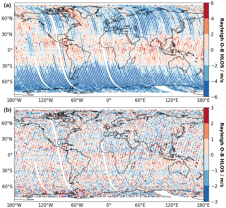
Figure 14Global distribution of the Rayleigh clear E(O−B) HLOS values, vertically averaged over all range gates, before (a) and after (b) the M1 bias correction. A total of 1 week of data (111 orbits, only ascending orbits) from 15 to 22 August 2019 is shown. The gaps are due to calibration procedures such as “hot-pixel-related” calibration measurements or calibration measurements of the internal path.
Already shortly after the successful launch of the Aeolus satellite in 2018, the operational assimilation of Aeolus wind products started at ECMWF in January 2020. A major milestone on the road to this achievement was the identification and correction of one of the most important systematic error sources for the Aeolus wind measurements. It was found that small temperature variations of about 0.3 ∘C across the primary M1 mirror of the Aeolus telescope lead to varying wind errors along the orbit of up to 8 m s−1. This paper presents a detailed characterization of the telescope-induced wind bias, describes the approach to correct for this bias source and discusses the performance of the bias correction based on data between June and December 2019.
Our analyses have shown that the orbital variation in the Rayleigh wind bias changes over seasons and, on top of that, strongly depends on the atmospheric scene. It turned out that the observed bias patterns are highly correlated with the temperatures measured at the primary telescope mirror. The telescope temperatures vary along the orbit as a result of changing TOA short- and longwave radiation of the Earth and the response of the telescope's thermal control system to that. The temperature changes affect the shape of the primary mirror which changes the focus of the telescope, and it is assumed that this leads to a change in the angle of incidence of the incoming light at the spectrometers of the instrument and hence to a wind bias. Moreover, it was found that the sensitivity of the Mie bias on the M1 temperatures is ∼ 10 times less than for the Rayleigh channel.
To correct for the M1 temperature effect a dedicated operational software was developed which describes the wind bias as a function of the M1 telescope temperature in a multiple linear regression (MLR) model. This approach is based on ECMWF model-equivalent HLOS winds as a bias-free reference and has been used operationally successfully at ECMWF since April 2020. The software uses 24 h of past data to derive the model fit coefficients and is updated twice per day. In this way, also the slowly drifting constant part of the wind bias can be corrected. It was demonstrated that the bias correction is capable of removing a large part of the M1-induced wind bias. In periods when the M1 influence on the wind bias is particularly strong, the bias correction can improve the SD(E(O−B)) value of the Rayleigh clear HLOS winds by up to 53 % from 2.89 to 1.36 m s−1. The remaining residual bias variation is considered to be of a mostly random nature and does not contain any obvious regular patterns. Moreover, the bias correction approach was also tested under special conditions during M1 optimization tests with changed thermal control law coefficients for the thermal control of the telescope. The results proved the reliability of the bias correction method even under these circumstances, paving the way for further in-orbit tests to improve the thermal control system of the telescope.
Despite the fact that on average the global bias of the u components of the ECMWF model with respect to radiosonde observations is smaller than 0.3 m s−1, the use of the numerical weather prediction model as a bias reference in the linear regression model is not ideal. Thus, this paper also presents the alternative of using ground return winds as a bias reference. The availability of ground returns is mainly restricted to polar regions with high surface albedo, which makes the task of bias modeling based on this more challenging. Hence, a downsized MLR approach with fewer independent variables is introduced. The results show that the approach based on ground return winds also reduces most of the M1-induced bias variations and performs in most cases only slightly worse than the operational ECMWF model-based approach. However, it was also shown that the performance of the ground return approach on average is 10.8 % worse than the ECMWF model-based bias correction, with maximum deviations of up to 25.6 %. Thus, it was decided to use ECMWF model winds as a bias reference. Nevertheless, the goal is to remove the model dependence in the calculation of winds, so for the future, further improving the performance of the ground-return-based approach and using it for upcoming reprocessing campaigns or even in the near-real-time-processing of the Aeolus products are planned. In addition, more sophisticated regression models, such as random forests (Svetnik et al., 2003) or generalized additive models (Hastie and Tibshirani, 1986), will be tested to further improve the performance of the M1 bias correction. With the knowledge obtained during this study, it will be possible in principle to improve both the thermal design of the telescope and the optical setup to reduce the bias contributions from the telescope temperature variation for a potential follow-on wind lidar mission. The goal would be to base the bias correction on measured ground return speeds, as was also initially foreseen for Aeolus.
The L1B products are processed in the framework of the second Aeolus reprocessing campaign and are available on the ADDF dissemination server under https://aeolus-ds.eo.esa.int/oads/access/collection/L1B_Wind_Products/tree (last access date: 15 November 2021) (ESA, 2021). The CDR OLR data are available at the NOAA National Climatic Data Center (https://doi.org/10.7289/V5SJ1HH2, Lee and NOAA CDR Program, 2011).
FW performed the data analysis and prepared the manuscript. MR, TK and LI largely contributed to the development of the presented methods and the operational M1 bias correction. EC is the thermal engineer of Aeolus at ESA-ESTEC and provided valuable input to improve the understanding of the thermal control of the telescope. JdK is the developer of the L2B processor and adapted the software for the M1 bias correction. NO analyzed the relationship between outgoing longwave radiation and the M1 radial temperature gradient. OR is the scientific coordinator of the Aeolus DISC and supported the investigation. All authors reviewed the initial draft version of the manuscript and helped to continuously improve the manuscript.
The contact author has declared that neither they nor their co-authors have any competing interests
The processor
development, improvement and product reprocessing preparation are performed
by the Aeolus DISC (Data, Innovation and Science Cluster), which involves
DLR, DoRIT, ECMWF, KNMI, CNRS/Météo-France, S&T, ABB
and Serco, in close cooperation with the Aeolus PDGS (Payload Data Ground
Segment). The analysis has been performed in the frame of the Aeolus DISC.
Publisher’s note: Copernicus Publications remains neutral with regard to jurisdictional claims in published maps and institutional affiliations.
This article is part of the special issue “Aeolus data and their application (AMT/ACP/WCD inter-journal SI)”. It is not associated with a conference.
The authors thank the Aeolus Space and Ground Segment Operations teams, the Aeolus Data Innovation and Science Cluster, and the technology centers at Airbus Defence and Space and ESA for their innovative spirit. The authors thank Gerhard Ehret for the internal review of this manuscript.
The article processing charges for this open-access publication were covered by the German Aerospace Center (DLR).
This paper was edited by Simone Lolli and reviewed by Hui Liu and two anonymous referees.
Andersson, E.: Statement of Guidance for Global Numerical Weather Prediction (NWP), World Meteorological Society, available at: https://docplayer.net/194586713-Statement-of-guidance-for-global-numerical-weather-prediction-nwp.html (last access date: 15 November 2021), 2018.
Ansmann, A., Wandinger, U., Rille, O. L., Lajas, D., and Straume, A. G.: Particle backscatter and extinction profiling with the spaceborne high-spectral-resolution Doppler lidar ALADIN: methodology and simulations, Appl. Optics, 46, 6606–6622, https://doi.org/10.1364/AO.46.006606, 2007.
Bell, W., English, S. J., Candy, B., Atkinson, N., Hilton, F., Baker, N., Swadley, S. D., Campbell, W. F., Bormann, N., Kelly, G., and Kazumori, M.: The Assimilation of SSMIS Radiances in Numerical Weather Prediction Models, IEEE T. Geosci. Remote, 46, 884–900, https://doi.org/10.1109/TGRS.2008.917335, 2008.
Belova, E., Kirkwood, S., Voelger, P., Chatterjee, S., Satheesan, K., Hagelin, S., Lindskog, M., and Körnich, H.: Validation of Aeolus winds using ground-based radars in Antarctica and in northern Sweden, Atmos. Meas. Tech., 14, 5415–5428, https://doi.org/10.5194/amt-14-5415-2021, 2021.
Chanin, M. L., Garnier, A., Hauchecorne, A., and Porteneuve, J.: A Doppler lidar for measuring winds in the middle atmosphere, Geophys. Res. Lett., 16, 1273–1276, https://doi.org/10.1029/GL016i011p01273, 1989.
Dabas, A., Denneulin, M. L., Flamant, P., Loth, C., Garnier, A., and Dolfi-Bouteyre, A.: Correcting winds measured with a Rayleigh Doppler lidar from pressure and temperature effects, Tellus A, 60, 206–215, https://doi.org/10.1111/j.1600-0870.2007.00284.x, 2008.
ESA: The four Candidate Earth Explorer Core Missions – Atmospheric Dynamics Mission, available at: https://earth.esa.int/eogateway/documents/20142/37627/The four Candidate Earth Explorer Core Missions - Atmospheric Dynamics Mission?text=worldview-3 (last access: 15 November 2021), 1999.
ESA: ADM-Aeolus Science Report, European Space Agency, SP-1311, ISBN 978-92-9221-404-3, ISSN 0379-6566, available at: https://esamultimedia.esa.int/multimedia/publications/SP-1311/SP-1311.pdf (last access: 15 November 2021), 2008.
ESA: Aeolus Online Dissemination System, ESA [data set], available at: https://aeolus-ds.eo.esa.int/oads/access/collection/L1B_Wind_Products/tree, last access: 15 November 2021.
Flamant, P., Cuesta, J., Denneulin, M.-L., Dabas, A., and Huber, D.: ADM-Aeolus retrieval algorithms for aerosol and cloud products, Tellus A, 60, 273–288, https://doi.org/10.1111/j.1600-0870.2007.00287.x, 2008.
Flament, T., Trapon, D., Lacour, A., Dabas, A., Ehlers, F., and Huber, D.: Aeolus L2A Aerosol Optical Properties Product: Standard Correct Algorithm and Mie Correct Algorithm, Atmos. Meas. Tech. Discuss. [preprint], https://doi.org/10.5194/amt-2021-181, in review, 2021.
Flesia, C. and Korb, C. L.: Theory of the double-edge molecular technique for Doppler lidar wind measurement, Appl. Optics, 38, 432–440, https://doi.org/10.1364/AO.38.000432, 1999.
Garnier, A. and Chanin, M. L.: Description of a Doppler rayleigh LIDAR for measuring winds in the middle atmosphere, Appl. Phys. B, 55, 35–40, https://doi.org/10.1007/BF00348610, 1992.
Guo, J., Liu, B., Gong, W., Shi, L., Zhang, Y., Ma, Y., Zhang, J., Chen, T., Bai, K., Stoffelen, A., de Leeuw, G., and Xu, X.: Technical note: First comparison of wind observations from ESA's satellite mission Aeolus and ground-based radar wind profiler network of China, Atmos. Chem. Phys., 21, 2945–2958, https://doi.org/10.5194/acp-21-2945-2021, 2021.
Hastie, T. and Tibshirani, R.: Generalized Additive Models, Statist. Sci., 1, 297–310, https://doi.org/10.1214/ss/1177013604, 1986.
James, G., Witten, D., Hastie, T., and Tibshirani, R.: An Introduction to Statistical Learning: with Applications in R, Springer, New York,426 pp., ISBN 978-1-0716-1305-4, 2014.
Kanitz, T., Lochard, J., Marshall, J., McGoldrick, P., Lecrenier, O., Bravetti, P., Reitebuch, O., Rennie, M., Wernham, D., and Elfving, A.: Aeolus first light: first glimpse, in: International Conference on Space Optics – ICSO 2018, International Conference on Space Optics – ICSO 2018, Chania, Greece, 111801R, https://doi.org/10.1117/12.2535982, 2019.
Korhonen, T., Keinanen, P., Pasanen, M., and Sillanpaa, A.: Polishing and testing of the 1.5 m SiC M1 mirror of the ALADIN instrument on the ADM-Aeolus satellite of ESA, in: Optical Fabrication, Testing, and Metrology III, Optical Fabrication, Testing, and Metrology III, 710219, https://doi.org/10.1117/12.797730, 2008.
Lee, H.-T. and NOAA CDR Program: NOAA Climate Data Record (CDR) of Daily Outgoing Longwave Radiation (OLR), NOAA National Climatic Data Center [data set], Version 1.2 olr-daily_v01r02_20190101_20191231.nc, https://doi.org/10.7289/V5SJ1HH2, 2011.
Lux, O., Wernham, D., Bravetti, P., McGoldrick, P., Lecrenier, O., Riede, W., D'Ottavi, A., Sanctis, V. D., Schillinger, M., Lochard, J., Marshall, J., Lemmerz, C., Weiler, F., Mondin, L., Ciapponi, A., Kanitz, T., Elfving, A., Parrinello, T., and Reitebuch, O.: High-power and frequency-stable ultraviolet laser performance in space for the wind lidar on Aeolus, Opt. Lett., 45, 1443–1446, https://doi.org/10.1364/OL.387728, 2020a.
Lux, O., Lemmerz, C., Weiler, F., Marksteiner, U., Witschas, B., Rahm, S., Geiß, A., and Reitebuch, O.: Intercomparison of wind observations from the European Space Agency's Aeolus satellite mission and the ALADIN Airborne Demonstrator, Atmos. Meas. Tech., 13, 2075–2097, https://doi.org/10.5194/amt-13-2075-2020, 2020b.
Lux, O., Lemmerz, C., Weiler, F., Kanitz, T., Wernham, D., Rodrigues, G., Hyslop, A., Lecrenier, O., McGoldrick, P., Fabre, F., Bravetti, P., Parrinello, T., and Reitebuch, O.: ALADIN laser frequency stability and its impact on the Aeolus wind error, Atmos. Meas. Tech., 14, 6305–6333, https://doi.org/10.5194/amt-14-6305-2021, 2021.
Malardel, S., Wedi, N., Deconinck, W., Diamantakis, M., Kuehnlein, C., Mozdzynski, G., Hamrud, M., and Smolarkiewicz, P.: A new grid for the IFS, ECMWF, 146, 23–28, https://doi.org/10.21957/zwdu9u5i, 2016.
Martin, A., Weissmann, M., Reitebuch, O., Rennie, M., Geiß, A., and Cress, A.: Validation of Aeolus winds using radiosonde observations and numerical weather prediction model equivalents, Atmos. Meas. Tech., 14, 2167–2183, https://doi.org/10.5194/amt-14-2167-2021, 2021.
McKay, J. A.: Modeling of direct detection Doppler wind lidar. II. The fringe imaging technique, Appl. Opt., 37, 6487–6493, https://doi.org/10.1364/AO.37.006487, 1998.
Reitebuch, O.: The Spaceborne Wind Lidar Mission ADM-Aeolus, in: Atmospheric Physics: Background – Methods – Trends, edited by: Schumann, U., Springer, Berlin, Heidelberg, 815–827, https://doi.org/10.1007/978-3-642-30183-4_49, 2012a.
Reitebuch, O.: Wind Lidar for Atmospheric Research, in: Atmospheric Physics: Background – Methods – Trends, edited by: Schumann, U., Berlin, Heidelberg, 487–507, https://doi.org/10.1007/978-3-642-30183-4_49, 2012b.
Reitebuch, O., Huber, D., and Nikolaus, I.: ADM-Aeolus, Algorithm Theoretical Basis Document (ATBD), Level1B Products, DLR Oberpfaffenhofen, available at:https://earth.esa.int/eogateway/documents/20142/37627/Aeolus-L1B-Algorithm-ATBD.pdf (last access: 15 November 2021), 2018a.
Reitebuch, O., Marksteiner, U., Rompel, M., Meringer, M., Schmidt, K., Huber, D., Nikolaus, I., Dabas, A., Marshall, J., de Bruin, F., Kanitz, T., and Straume, A.-G.: Aeolus End-To-End Simulator and Wind Retrieval Algorithms up to Level 1B, EPJ Web Conf., 176, 02010, https://doi.org/10.1051/epjconf/201817602010, 2018b.
Reitebuch, O., Marksteiner, U., Weiler, F., Lemmerz, C., Witschas, B., Lux, O., Meringer, M., Schmidt, K., Huber, D., Dabas, A., Flament, T., Stieglitz, H., Mahfouf, J.-F., Isaksen, L., Rennie, M., Stoffelen, A., Marseille, G., Kloe, J., Donovan, D., and Lodovico, I.: The Aeolus Data Innovation and Science Cluster DISC – Overview and First Results, ESA Living Planet Symposium, Milan, Italy, 13–17 May 2019, 2019.
Reitebuch, O., Lemmerz, C., Lux, O., Marksteiner, U., Rahm, S., Weiler, F., Witschas, B., Meringer, M., Schmidt, K., Huber, D., Nikolaus, I., Geiss, A., Vaughan, M., Dabas, A., Flament, T., Stieglitz, H., Isaksen, L., Rennie, M., Kloe, J. de, Marseille, G.-J., Stoffelen, A., Wernham, D., Kanitz, T., Straume, A.-G., Fehr, T., Bismarck, J. von, Floberghagen, R., and Parrinello, T.: Initial Assessment of the Performance of the First Wind Lidar in Space on Aeolus, EPJ Web Conf., 237, 01010, https://doi.org/10.1051/epjconf/202023701010, 2020.
Rennie, M. P.: An assessment of the expected quality of Aeolus Level-2B wind products, EPJ Web Conf., 176, 02015, https://doi.org/10.1051/epjconf/201817602015, 2018.
Rennie, M. and Isaksen, L.: The NWP impact of Aeolus Level-2B Winds at ECMWF, ECMWF Technical Memoranda, technical report, 110 pp., https://doi.org/10.21957/alift7mhr, 2020.
Rennie, M., Tan, D., Poli, P., Dabas, A., De Kloe, J., Marseille, G.-J., and Stoffelen, A.: Aeolus Level-2B Algorithm Theoretical Basis Document, ECMWF, available at: https://earth.esa.int/eogateway/documents/20142/37627/Aeolus-L2B-Algorithm-ATBD.pdf (last access: 15 November 2021), 2020.
Rennie, M. P., Isaksen, L., Weiler, F., de Kloe, J., Kanitz, T., and Reitebuch, O.: The impact of Aeolus wind retrievals on ECMWF global weather forecasts, Q. J. Roy. Meteor. Soc., 147, 3555–3586, https://doi.org/10.1002/qj.4142, 2021.
Stoffelen, A., Pailleux, J., Källén, E., Vaughan, J. M., Isaksen, L., Flamant, P., Wergen, W., Andersson, E., Schyberg, H., Culoma, A., Meynart, R., Endemann, M., and Ingmann, P.: The Atmospheric Dynamics Mission for global wind field measurement, B. Am. Meteorol. Soc., 86, 73–88, https://doi.org/10.1175/BAMS-86-1-73, 2005.
Stoffelen, A., Benedetti, A., Borde, R., Dabas, A., Flamant, P., Forsythe, M., Hardesty, M., Isaksen, L., Källén, E., Körnich, H., Lee, T., Reitebuch, O., Rennie, M., Riishøjgaard, L.-P., Schyberg, H., Straume, A. G., and Vaughan, M.: Wind Profile Satellite Observation Requirements and Capabilities, B. Am. Meteorol. Soc., 101, E2005–E2021, https://doi.org/10.1175/BAMS-D-18-0202.1, 2020.
Straume, A. G.: Aeolus Sensor and Product Description, European Space Agency, available at: https://earth.esa.int/pi/esa?type=file&table=aotarget&cmd=image&alias=Aeolus_Sensor_Processing_and_Product_Description, last access: 15 November 2021, 2018.
Svetnik, V., Liaw, A., Tong, C., Culberson, J. C., Sheridan, R. P., and Feuston, B. P.: Random Forest: A Classification and Regression Tool for Compound Classification and QSAR Modeling, J. Chem. Inf. Comp. Sci., 43, 1947–1958, https://doi.org/10.1021/ci034160g, 2003.
Tan, D. G. H., Andersson, E., Kloe, J. D., Marseille, G.-J., Stoffelen, A., Poli, P., Denneulin, M.-L., Dabas, A., Huber, D., Reitebuch, O., Flamant, P., Rille, O. L., and Nett, H.: The ADM-Aeolus wind retrieval algorithms, Tellus A, 60, 191–205, https://doi.org/10.1111/j.1600-0870.2007.00285.x, 2008.
Weiler, F.: Bias correction using ground echoes for the airborne demonstrator of the wind lidar on the ADM-Aeolus mission, Master Thesis, University of Innsbruck, Innsbruck, 89 pp., available at: https://diglib.uibk.ac.at/ulbtirolhs/content/structure/2143358 (last access: 15 November 2021), 2017.
Weiler, F., Kanitz, T., Wernham, D., Rennie, M., Huber, D., Schillinger, M., Saint-Pe, O., Bell, R., Parrinello, T., and Reitebuch, O.: Characterization of dark current signal measurements of the ACCDs used on board the Aeolus satellite, Atmos. Meas. Tech., 14, 5153–5177, https://doi.org/10.5194/amt-14-5153-2021, 2021.