Unravelling a black box: an open-source methodology for the field calibration of small air quality sensors

The last 2 decades have seen substantial technological advances in the development of low-cost air pollution instruments using small sensors. While their use continues to spread across the field of atmospheric chemistry, the air quality monitoring community, and for commercial and private use, challenges remain in ensuring data quality and comparability of calibration methods. This study introduces a seven-step methodology for the field calibration of low-cost sensor systems using reference instrumentation with user-friendly guidelines, open-access code, and a discussion of common barriers to such an approach. The methodology has been developed and is applicable for gas-phase pollutants, such as for the measurement of nitrogen dioxide (NO₂) or ozone (O₃). A full example of the application of this methodology to a case study in an urban environment using both multiple linear regression (MLR) and the random forest (RF) machine-learning technique is presented with relevant R code provided, including error estimation. In this case, we have applied it to the calibration of metal oxide gas-phase sensors (MOSs). Results reiterate previous findings that MLR and RF are similarly accurate, though with differing limitations. The methodology presented here goes a step further than most studies by including explicit transparent steps for addressing model selection, validation, and tuning, as well as addressing the common issues of autocorrelation and multicollinearity. We also highlight the need for standardized reporting of methods for data cleaning and flagging, model selection and tuning, and model metrics. In the absence of a standardized methodology for the calibration of low-cost sensor systems, we suggest a number of best practices for future studies using low-cost sensor systems to ensure greater comparability of research.

1 Introduction

Air pollution remains a leading cause of premature death globally (Landrigan et al., 2018). The recent trend in air pollution research of using low-cost sensors (LCSs) to measure common gas-phase and particulate air pollutants (e.g. CO, NO_x, O₃, PM) is an attempt to close gaps in our understanding of air pollution and make its measurement cheaper, widespread, and more accessible (Kumar et al., 2015; Lewis et al., 2016, 2018). The development of these new technologies represents a paradigm shift that has opened up air pollution monitoring to a much wider audience (Morawska et al., 2018; Snyder et al., 2013). In recent years, LCSs have been used to develop or supplement existing air pollution monitoring networks to provide higher spatial resolution (e.g. CitiSense, U.S. EPA Village Green), as well as in a citizen science context to report on and share information about air quality (e.g. AirVisual, Purple Air) (Morawska et al., 2018; Muller et al., 2015). Projects like these are a promising step towards empowering citizens with greater knowledge of their local air quality.

However, as there are myriad commercially available LCSs that use a variety of sensors and have substantial differences in quality, standardizing their application remains challenging and urgent (Karagulian et al., 2019). In measuring gas-phase pollutants, for example, metal oxide sensors (MOSs) and electrochemical sensors (ECs) are often used, although they have different limits of detection and cross-sensitivities that need to be taken into account (Lewis et al., 2016, 2018; Rai et al., 2017). Under ambient conditions, the performance of these two sensor types varies substantially, with some studies reporting moderate to good agreement with concentrations measured by reference instrumentation, whereas others find very poor agreement (Lewis et al., 2018). A further challenge is that many LCSs are in the form of small sensor systems ¹ sold as ready-to-use products to customers, most often using a “black box” proprietary calibration algorithm for producing concentrations which, along with raw data, is not publicly available (Karagulian et al., 2019). Furthermore, a wide range of calibration techniques have been applied to LCSs in field studies, but lack uniformity in metrics used, experimental setup, reference equipment, and environmental conditions, making it difficult to draw conclusions about their overall performance (Karagulian et al., 2019; Rai et al., 2017).

In general, pairwise reference calibration has been done on an individual sensor system basis as well as a sensor system cluster basis, also known as “sensor fusion” (Barcelo-Ordinas et al., 2019). The former tends to be more accurate but becomes logistically and computationally intensive for large numbers of LCSs and is more sensitive to sensor decay and medium-scale drift. The latter has been shown to be effective at calibrating groups of sensors when using the median sensor signal of a co-located cluster of sensors to develop a single calibration model applicable to all sensors (Smith et al., 2017, 2019). Using a cluster-based approach has been shown to produce calibration factors that may be more robust over longer time frames but have higher margins of error for individual sensors. Both methods have their advantages and disadvantages that must be balanced based on the desired application for the sensor systems. Further methods for calibration beyond pairwise reference calibration include node-to-node calibration (Kizel et al., 2018) or proxy calibration (Miskell et al., 2018).

Previous research has used linear regression, multiple linear regression (MLR), and machine-learning techniques such as random forest (RF), artificial neural networks (ANNs), and support vector regression (SVR) to calibrate LCSs with reference instrumentation for gas-phase pollutants. Here too, there is a lack of standardization, as MLR, RF, ANN, and SVR have all been found to be the most accurate method across various studies (Bigi et al., 2018; Cordero et al., 2018; Hagan et al., 2018; Karagulian et al., 2019; Lewis et al., 2016; Malings et al., 2019; Smith et al., 2019; Zimmerman et al., 2018). Only linear regression has been consistently identified as an unsuitable model, largely because it fails to take into account cross-sensitivities and environmental influences on sensor functioning and because sensor responses are often non-linear. For this same reason, nonparametric methods such as the aforementioned machine-learning techniques tend to be more accurate, as they are better at modelling non-linear sensor responses while being able to better take into account interferences in sensor functioning (Barcelo-Ordinas et al., 2019; Karagulian et al., 2019). However, it must be said that any of these statistical methods can be applied as long as they properly account for autocorrelation, multicollinearity, and non-linearity in the data with relevant transformations.

There are several key issues with previous work on calibrating LCS that must be acknowledged. First, the metrics used to report model suitability vary substantially. Karagulian et al. (2019) found in their comprehensive review of the LCS literature that only the coefficient of determination (R²) was applicable for cross-comparison of all studies. While this metric can be useful in measuring the agreement between LCS data and reference measurements, it does not give a sense of the model error. Future studies should, at a minimum, report R², root-mean-square error (RMSE), and mean average error (MAE) when discussing calibration performance (Barcelo-Ordinas et al., 2019; Karagulian et al., 2019). Second, while there are many studies that calibrate LCSs with MLR or machine-learning techniques, the associated model selection, validation, and tuning methods are rarely reported. The latter of these is especially important for machine-learning (ML) techniques with many tuning parameters, where the problem of over-fitting is more common. Some studies do report steps for model validation (Hagan et al., 2018; Spinelle et al., 2015; Zimmerman et al., 2018) or model tuning (Bigi et al., 2018; Spinelle et al., 2015), but they do not go into depth as to how these were determined or optimized. Especially with “black box” techniques such as ANN, SVR, or RF, reporting steps taken to validate the model and optimize parameters are crucial to ensuring consistency among studies. Last, the issues of multicollinearity and autocorrelation, which are common among LCS time series data and of substantial importance when using MLR, are rarely addressed. If at all mentioned, they are referred to as being better handled by non-linear ML techniques such as SVR or RF (Bigi et al., 2018) or as potentially obscuring the statistical significance of models (Masiol et al., 2018). This study seeks to take a step forward in ensuring these issues are addressed in future LCS calibration studies.

In the absence of a standardized calibration methodology, the ever-growing body of LCS literature will continue to be largely incomparable, with research running in parallel using varied methods. Though several comprehensive reviews of LCSs which establish helpful guidelines for their use have been completed (Lewis et al., 2018; Williams et al., 2014), best practices for calibration with reference instruments that should be undertaken in any field deployment were not specifically reported. More recently, Barcelo-Ordinas et al. (2019) published an extensive study on the calibration of LCSs, including some general calibration guidelines. While these are a helpful guide for calibration methodologies, they lack important details on the post-processing of data during the model-building process. This study seeks to expand upon this work and specifically address the standardization of individual pairwise calibration of LCSs housed in sensor systems with reference instrumentation by presenting user-friendly guidelines, open-access code, and a discussion of common barriers to field calibration. With the publication of this step-by-step methodology for the statistical calibration of low-cost sensor systems, we hope to establish a framework from which calibration methods can be better compared.

2 Methods

The following section outlines a methodology for the deployment and field calibration of LCSs for the measurement of gas-phase pollutants. First, some key considerations for the experimental deployment of small sensor systems will be discussed. Second, a seven-step statistical calibration methodology for the post-processing of data will be described. Last, an example of the use of this methodology, for both deployment and calibration, using data collected during a measurement campaign in 2017 and 2018, is provided (Sect. 3).

For this methodology, it is important to first establish under which circumstances the following steps would apply. This is a reference-based pairwise method for the individual calibration of small sensor systems, and therefore the user will need to have access to reference instrumentation with which the small sensor systems can be co-located, whether their own or in collaboration with for example a city monitoring network. This makes the methodology inapplicable for individual users in a citizen science context who may not have access to reference instrumentation. These reference instruments should adhere to standardized guidelines on accuracy (i.e. EU Air Quality Directive (2008/50/EC), US National Ambient Air Quality Standards (NAAQS)). A co-location in this sense refers to the installation of the small sensor systems in the close vicinity (ca. 1–3 m) of the reference instruments, so that they receive the same parcels of air. This paper focuses on the usage of field (i.e. in situ) co-locations in calibrating small sensor systems. If access to reference data or the raw small sensor data is not possible, then this methodology cannot be applied. Furthermore, while it was applied here to sensor systems containing metal oxide LCSs, this methodology is also equally as applicable to electrochemical (EC) LCSs or photoionization detectors (PIDs), as these produce a similar measure of voltage that varies in response to changing concentrations of gas-phase species and have similar cross-sensitivities to temperature and relative humidity. It is not directly applicable for optical particle counters (OPCs) for the measurement of particulate matter, as the transformation of the raw data into concentrations during calibration functions differently, though some of the principles discussed here are still relevant. For an application of this methodology to EC sensors, please see Schmitz et al. (2021).

2.1 Key considerations for the experimental deployment of small sensor systems

When calibrating small sensor systems, the experimental deployment and co-location of devices is a key step with several important considerations that must be accounted for. First, the co-location with reference instrumentation should ideally occur at the same test site where the small sensor systems are to be deployed. If unfeasible for logistical reasons, an analogue site should be selected. Criteria for analogue selection entail similar characteristics as those for test site selection. The analogue site should (1) have similar sources and ranges of concentrations of air pollutants as the test site, (2) experience comparable meteorological conditions and similar circulation dynamics, and (3) be physically located in the same region as the test site. While it is unlikely that there will be a perfect analogue site, any field calibration should take these criteria into consideration in order to enhance validity of experimental results.

Second, the frequency and timing of co-locations should reflect site-specific variations in meteorological conditions. Generally, these should be done often enough so that co-location data cover similar ranges of meteorological conditions and concentrations of air pollutants as the experimental data, but not so often that there is a concomitant loss of experimental data. A rule of thumb for long-term experiments (>6 months) in temperate seasonal environments is a 2-week co-location every 2–3 months. For short- to medium-term experiments, a 2-week co-location before and after and perhaps one in-between, depending on changes in meteorological conditions, should suffice. Regular co-location allows for the establishment of datasets that cover not only changes in meteorology but also sensor functioning and interactions of potentially cross-sensitive species. If these considerations are taken into account during the experimental deployment, the likelihood that these datasets will be of good quality will be higher. In this study, we focus primarily on stationary field deployment of low-cost sensor systems. There are, however, other forms of deployment, including indoor and mobile, for which these criteria also apply. It is important to mention that there may be other considerations required in such alternative forms of deployment, e.g. more scrutinous data cleaning in mobile deployments due to impacts of rapidly changing environments on sensor performance.

2.2 The seven-step statistical calibration method

Raw data from small sensor systems, if treated and transformed properly, can provide informative air pollutant concentrations. This treatment must, however, be rigorous if the resultant concentrations are to be used in further analysis. This section provides a general description of a seven-step methodology for the post-processing and calibration of LCS data gathered with small sensor systems (see Fig. 1). Multiple linear regression (MLR) and random forest (RF) were selected as calibration methods to be used in this methodology, although it can be generally applied to other regression or machine learning methods. Information on the functions and packages from the open-source R statistical software program (R Core Team, 2019) used in this methodology is provided for each step. This information and the code can be found in the open-source repository Zenodo (see below for DOI).

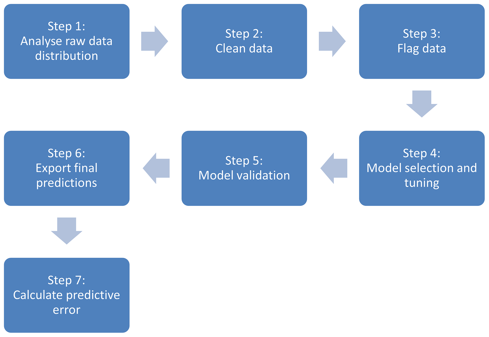
Figure 1 Schematic representation of the seven-step calibration method for processing small sensor system data.

2.2.1 Step 1: analyse and understand raw data distribution

The first step is to gain a general understanding of the data. Specifically, establishing an overview of data distributions and potential data quality issues (data gaps, presence of outliers, changes in baselines, etc.) is helpful for identifying problems and solutions during calibration. It should also be checked that all associated metadata are available for all datasets.

In this study, all variables that were to be used in model selection were assessed in this step. For example, the distributions of the reference concentrations, small sensor system raw data, and meteorological variables from the co-location and experimental datasets were analysed. Meteorological variables including temperature, relative humidity, and wind speed and direction across the co-location and experimental datasets were compared. Additional variables that could be considered but were not analysed here include precipitation, boundary layer height, and insolation, among others. A visual assessment of these data using histograms, violin plots, and time series plots was conducted. This step provided information about the structure of each available co-location dataset and the experimental dataset crucial to decision-making in later steps.

2.2.2 Step 2: data cleaning

Next, the datasets should be cleaned of erroneous outliers and unreliable data. This step is crucial, as outliers can have a particularly strong effect on calibration models and especially so on linear regression models.

To accomplish this, the time series plots generated in step 1 were first used to visually evaluate the data. Sequence outliers resultant from sensor warm-up time or sensor malfunctioning were identified and removed using an automated function. Next, an algorithm was tested, trained, and implemented that uses a simple z test with a running mean and standard deviation to detect point outliers resultant from instrument measurement error. Tests of normality with datasets greater than 50 points are irrelevant in determining whether parametric tests can be used or not (Ghasemi and Zahediasl, 2012). Analysis of the data in this study revealed the same, as data segments of fewer than 30 points consistently passed the Shapiro–Wilk test, but with progressively larger data segments, more and more of the data failed the test. Therefore, it was assumed that the data aligned enough with the normal distribution for this test to apply. The size of the moving time frame from which the running mean and standard deviation were calculated and the z-score threshold used to designate “outlierness” were tested and optimized. Durations of 1, 2, 5, 10, 30, 60, 120, and 300 min were considered for the moving window and thresholds of 3, 4, 5, and 6 were tested. This was done for each variable individually. The points flagged as outliers with this method were then graphically assessed against neighbouring data points to prevent inadvertent removal of peak emission events. In other cases where assessing all outliers is impractical, it is recommended to do so with a random subset of outliers. Furthermore, if substantial short-term events are expected due to the deployment environment, such as during mobile measurements, a more thorough check of potential outliers should be done. Other outlier detection functions using autoregressive integrated moving average (ARIMA) and median absolute deviation (MAD) were tested and were found to be inappropriate for these data.

2.2.3 Step 3: flag data for further scrutiny

Experimental data outside the range of the co-location data (i.e. beyond the minimum and maximum values) should be flagged as they may be less reliably predicted than those which are in range and should be given a higher level of uncertainty (Smith et al., 2019). Flagging such data points strikes a balance between removing them from the analysis and highlighting their associated uncertainty.

Once flagged, these data points were treated differently in later analysis (Sect. 3.5). Similarly, co-location data outside the range of the experimental data received a flag. During the model selection process, these flags were used to remove data that may serve to bias the model. While this may seem unnecessary, if the experimental range of environmental conditions is much smaller than those of the co-locations, it could be that using a smaller, more comparable range of co-location data is more suitable for model selection. This is data and model dependent, however, and was therefore tested in Step 6.

2.2.4 Step 4: model selection and tuning

Model selection and tuning is a seldom-reported step that is vital in ensuring the calibration model is suitable for use. Rigorously scrutinizing a variety of potential models and optimizing their parameters provides reproducible justification for the final model selected. This is particularly important for machine-learning techniques which can have a wide array of parameters for tuning model performance. Furthermore, appropriate methods used in model selection ensure that problems of multicollinearity and autocorrelation can be corrected for, as superfluous predictors suffering from these issues will be identified and removed. Before building and selecting potential models, the relationships between predictors and response variable, including potential transformations, must be determined. This is important for linear regression models but is not relevant for ML techniques which do not take these transformations into account. Often the sensor specifications indicate what type of transformation (exponential, log-linear, etc.) may be necessary.

The co-location data were used in this step to train various models and determine the best-fitting MLR and RF models. In this case, log transformations were recommended for the MOSs used but were cross-checked with other common transformations including log-log, square-root, and inverse. Model selection proceeded through backwards selection using the coefficient of determination (R²), root-mean-squared error (RMSE), and Akaike information criterion (AIC) (Akaike, 1973) for MLR or variable importance (VI) (Breiman, 2001) for RF as criteria. To determine the best models, the training dataset was broken up into smaller sets by using a moving window of 4 d to train the models and the fifth day to test. The models with the best average RMSE over the various fifth day predictions were selected.

For RF the model parameters of mtry (the number of randomly selected variables at each node), min.node.size (the minimum number of data points in the final node), and splitrule (the method by which data are split at each node) were optimized by testing various combinations and selecting the most accurate in terms of RMSE, with data split in the same manner as for MLR. Subsequently, measures of AIC for the regression model and VI for the random forest model were assessed to determine which predictors should remain in the model. For MLR, this involved the repeated bootstrapping of the training set combined with stepwise selection, using the AIC to robustly determine predictor inclusion. The models were then finally tested on the test subset and assessed using RMSE and R². The most accurate MLR and RF models were then sent to the next step for validation.

2.2.5 Step 5: model validation

Model validation is often overlooked but is necessary to ensure that the most accurate model selected is reliable (i.e. has good predictive power for independent data). While a singular instance of splitting the dataset during the model selection process into training and testing subsets is one method of validating the model, an additional step ensures more rigorous validation.

In this case, to validate the MLR and RF models selected in Step 4, the co-location data were repeatedly split into training and testing subsets at a ratio of $\mathrm{75}/\mathrm{25}$. This was done by splitting the co-location training set into continuous blocks representing 25 % of the training data (in this case 6 d) as test subsets and using the rest of the co-location data to train the model. A robustness cross-check with various splitting ratios was conducted, and it was found that changing the splitting ratio did not significantly impact the results. Using continuous blocks instead of random sampling is necessary to account for the autocorrelation in the data (Carslaw and Taylor, 2009). The accuracy of the final models was then assessed on the continuous blocks using R², RMSE, and variable importance. These metrics were then graphed across all continuous blocks to assess model stability. In this case, instability refers to major differences in R² and RMSE between folds likely caused by differing field conditions among the training and test folds. If this is seen, it indicates that the model may be too sensitive to changes in field conditions. If the graphs showed instability across the various folds, Step 4 was repeated and a new model was selected for validation.

2.2.6 Step 6: export final predictions

Once the selected model has been validated, the next step in the process is to export predictions of the experimental data as concentrations. Only co-location data deemed relevant from Steps 1–3 should be used to train the model, which is then used to predict experimental concentrations.

In this case, the co-location data were used to train the best MLR and RF models identified in Steps 4 and 5. These models were then applied to the raw experimental data in order to predict final concentrations. The final predictions were then graphed and compared using time plots and histograms.

2.2.7 Step 7: calculate total predictive error

Last, it is vital that overall error and confidence intervals for the predictions are reported in this step. Most models have associated methods for reporting metrics such as standard error which can be used to establish confidence intervals around the predictions. Compounded to this must be the technical error associated with measurements from the reference instruments. Thus, the overall error should combine technical and statistical error.

In this study, to test the impact of the precision of the reference measurements on model accuracy, the reference NO₂ and O₃ data were smeared using a normal distribution with each point as the mean and each instrument's measure of imprecision as the standard deviation. Smearing refers to transforming the data by shifting the actual value within the range of uncertainty. This test therefore determined whether the imprecision given by each instrument's specifications should be factored into the overall predictive error. This was done over 50 iterations to see how model accuracy responded to shifts in reference concentrations within the margins of error. Co-location data were split $\mathrm{75}/\mathrm{25}$ into a training set and testing set, respectively. In each iteration, separate MLR and RF models for NO₂ and O₃ were trained; each was trained once with the reference measurements and once with smeared reference measurements. All models were then tested for predictive accuracy on the testing subset, to compare the impact of smeared versus measured reference data on model performance.

Last, the overall uncertainty was calculated. For the reference instruments, the technical measurement was taken from their specifications. This was added to the overall statistical error, for which the median MAE across all blocks from the model validation step was used. Both the MLR and RF models calculated a measure of standard error, which was compared with the combined uncertainty measure. The more appropriate of the two was then added to the final predictions from Step 6.

3 Example application of the methodology

3.1 Small sensor systems used

The small sensor systems used in this example are EarthSense Systems, Ltd. “Zephyr” prototypes², henceforth referred to as “Zephyrs”. This term refers to the whole small sensor system including housing, sensors, and GPS. Installed within the Zephyr prototypes were a number of metal oxide sensors (MOSs) that measure reducing gases, oxidizing gases (used here for detection of nitrogen dioxide), ozone, and ammonia, as well as a meteorological sensor for temperature and relative humidity; see Table 1 for more on these sensor specifications. These MOSs typically experience significant amounts of drift 4 months after initial calibration, which is why in this study co-locations were conducted at high frequency, before and after each experiment. For greater detail on the development, functioning, and operation of the sensors housed within these prototypes, see Peterson et al. (2017).

Table 1 Sensors installed within the EarthSense Zephyr prototypes. Table reproduced from Peterson et al. (2017).

3.2 Reference instruments

The reference instrumentation included a Teledyne model T-200 NO–NO₂–NO_x analyser and a 2B Technologies, Inc. ozone monitor. These instruments were intercompared with reference instruments – CAPS (Aerodyne, USA), CLD 770 AL ppt (ECO PHYSICS AG, Switzerland) and O242M (Environnement S.A., France) – from the Forschungszentrum Jülich as part of the measurement campaign and showed decent agreement (R²=0.70) for NO₂ and good agreement (R²=0.88) for O₃ (see Figs. S1–S3 in the Supplement). Ambient air temperature and relative humidity (Lambrecht, PT100) data one block away from the experimental site were provided by the Free University Berlin for two measurement campaigns (more information in Sect. 3.3). Wind speed and direction (Campbell Scientific, IRGASON) were measured 10 m above the roof of the main building of the Technical University Berlin (TUB) at Campus Charlottenburg, which is located across the street from the experimental site. This site is part of the Urban Climate Observatory (UCO) Berlin operated by the TUB for long-term observations of atmospheric processes in cities (Scherer et al., 2019a).

3.3 Experimental deployment

Measurements were conducted in a street canyon on the Charlottenburg Campus of the TUB, on the façade of the mathematics building (52^∘30${}^{\prime }{\mathrm{49.7}}^{\prime \prime }$ N, 13^∘19${}^{\prime }{\mathrm{34.5}}^{\prime \prime }$ E) as a part of several measurement campaigns of the joint project “Three-dimensional observation of atmospheric processes in cities” (3DO) (Scherer et al., 2019a), which was part of the larger research program Urban Climate Under Change [UC]² (Scherer et al., 2019b). The area directly around the measurement site consists of university buildings with a wide main thoroughfare (Strasse des 17. Juni) that runs from east to west through Berlin (see Fig. S6 in the Supplement). These occurred during two measurement campaigns which are henceforth referred to as the Summer Campaign (SC), which includes all 2017 measurements, and the Winter Campaign (WC), which includes the 2018 measurements, respectively (Fig. 2).

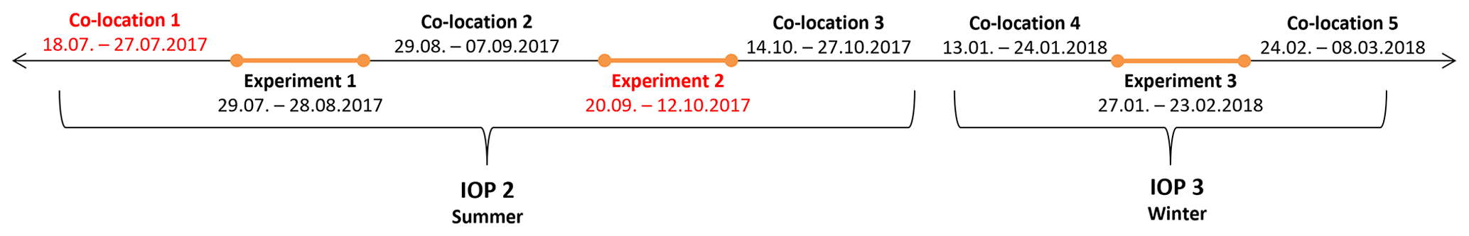
Figure 2 Timeline of SC and WC depicting the relationship between co-locations and experiments. Due to technical issues of individual instruments, data were unavailable for the segments marked in red.

For the field calibration the Zephyrs were co-located with the aforementioned reference instruments at the deployment site. The reference station for co-location was set up in an office on the sixth floor of the mathematics building on the south-facing façade that provided constant power for reference instrumentation and the Zephyrs, as well as space for air inlet tubing to be passed through the windows to the reference instrumentation (Fig. 3). The Zephyrs and the air inlets were attached next to each other on the same railing outside the office. This ensured that all instruments were receiving the same parcels of air throughout the co-location. One Zephyr was co-located with reference instrumentation throughout the summer campaign (s71) and one throughout the winter campaign (s72). The reference station measurements were continuous throughout the co-locations and the experiments. The experiments took place from 29 July–28 August and from 20 September–12 October in 2017 and from 27 January–23 February in 2018. Five co-locations were conducted in total across the two campaigns. These took place from 18 July–27 July, 29 August–7 September, and 14 October–27 October (all in 2017) during the SC and from 13 January–24 January and 23 February–8 March (both in 2018) during the WC. All dates refer to time frames of the data presented, as the first and last days of deployment or co-location were not used owing to different start and end times of installation, as well as sensor warm-up times. To compare sensor performance between s71 and s72, an intercomparison of available co-location raw data was conducted for the oxidizing MOS (Oxa) and ozone MOS (O3a). During all co-locations, the sensors had a linear relationship and an R²>0.95 (Figs. S4 and S5). In only one instance was this not the case (co-location 2, O3a), where the R² was 0.59 and a deviation from linearity was detected. This relationship was linear and normal in all other co-locations.

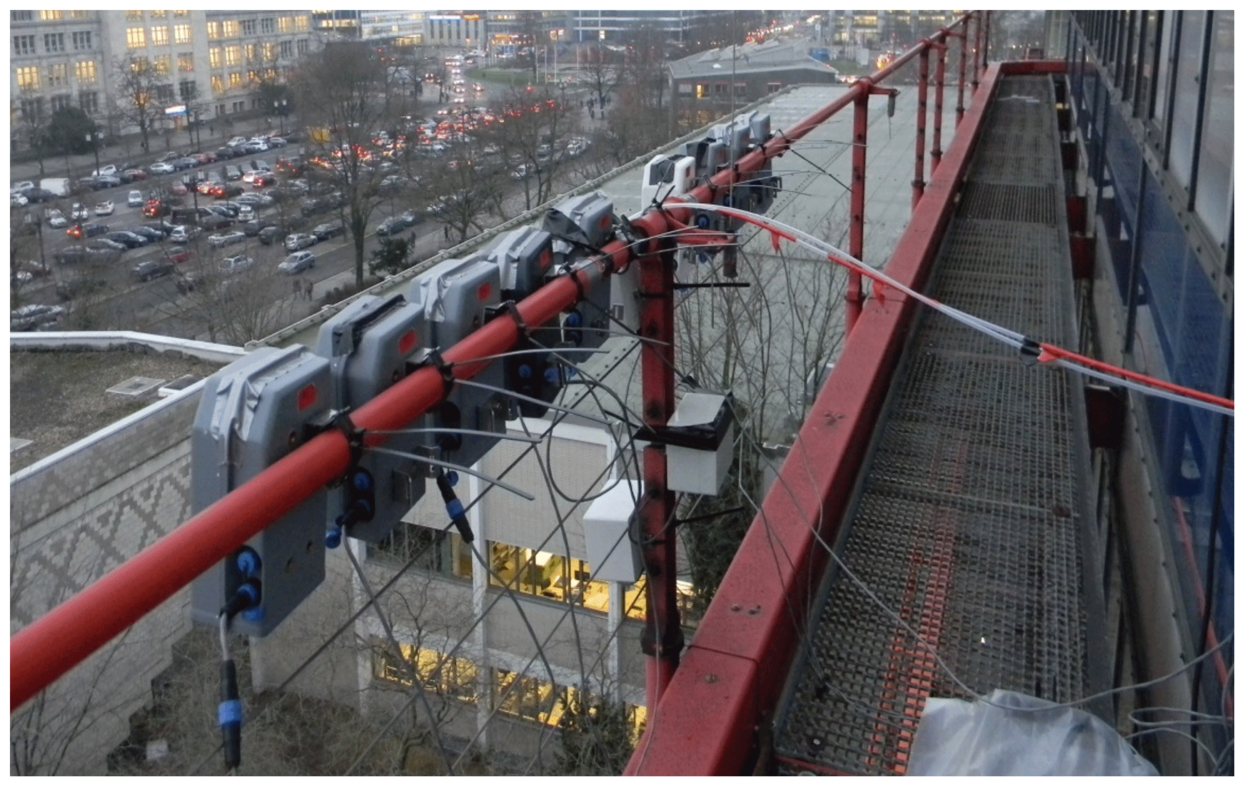
Figure 3 Set-up of the co-location of the prototype Zephyrs with reference instruments on the sixth floor of the mathematics building. The grey units are the Zephyrs, and the two inlet tubes connect to the reference devices located inside the office.

This example focuses on Zephyr s71 during the SC and Zephyr s72 during the WC. For the sake of brevity, all graphs and tables included in this section pertain only to the former. Those relevant for the latter can be found in the Supplement. Due to continuous co-location of these two sensors, the statistical models established using the seven-step method could be trained with co-location data and, atypically, assessed for their accuracy using reference concentrations during the entire experimental window. What follows is a thorough description of the application of the seven-step method for calibration.

In order to calibrate the Zephyrs, reference NO₂ and O₃ data, meteorological data, and raw data from the Zephyr sensors were used. Concentrations of NO₂ from the Teledyne T200 NO_x analyser and O₃ from the O3-2B Technologies instruments were used as response variables in the models. Ambient temperature (T_amb) and relative humidity (RH_amb) data as well as wind speed (ws) and direction (wd) data were tested as predictors in the statistical models. Four variables from the Zephyrs themselves were also tested in the statistical models as predictors: (1) Oxa, a measure of resistance from one MOS used to detect oxidizing substances (in this case NO₂); (2) O3a, another measure of resistance from a MOS that detects O₃; (3) a measure of temperature collected by the Zephyr (T_int); and (4) a measure of relative humidity collected by the Zephyr (RH_int). Finally, the binary time-of-day (ToD) variable was created to distinguish between night and day, as the chemistry of the analysed species changes significantly. Further reference data on other species would have been beneficial to this calibration, as the MOSs do exhibit cross-sensitivities to other species, but resources were insufficient, and these data were not collected.

3.4 Seven-step calibration of the Zephyrs

The temperature and relative humidity from the Zephyrs (T_int and RH_int) reflect the conditions within the sensor system and typically parallel ambient data, however, with an offset. These data are henceforth referred to as “internal” temperature and relative humidity. Throughout the example, both internal and ambient T and RH are used to assess their comparative influence on model accuracy. This was tested as ambient T and RH from reference instruments are not always available at experimental sites, whereas the internal T and RH of the Zephyrs are always available. The reference and meteorological data had an original time resolution of 1 min whereas the Zephyr data were collected at a time resolution of 10 s. Analysis during the seven-step process was conducted using 5 min averages except for outlier detection, which was done at original time resolution.

3.4.1 Step 1: analyse raw data distribution

The distributions of the reference, meteorological, and Zephyr data were first compared between each co-location individually, both co-locations together, and the experimental deployment data of Experiment 1. The violin plots of ambient RH and T, NO₂, and O₃ for co-location 2 (Fig. 4) show that the meteorological conditions and pollutant concentrations experienced were quite similar to those of the experiment. The ranges, median values, and the interquartile ranges are quite similar. This is further reflected by the similarity in distributions of both the Zephyr MOS data (Oxa and O3a) and the reference instrument data between the second co-location and the experiment.

Figure 4 Violin plots of (a) reference NO₂, (b) reference O₃, (c) Oxa, (d) O3a, (e) T_amb, (f) RH_amb, (g) T_int, and (h) RH_int for co-location 2, co-location 3, both co-locations combined, and the experimental data.

By contrast, the distributions of the same variables for the third co-location (Fig. 4) are demonstrably different from the other co-location and the experimental data. The ambient temperature and relative humidity conditions were significantly cooler and wetter in the third co-location than during the experiment, and the NO₂ and O₃ concentrations were much higher and lower, respectively. Furthermore, the MOS data in this co-location have a much different median and interquartile range (IQR) than the experiment, although the overall range is similar.

With both locations combined (Fig. 4), the distributions of all variables are representative of the experimental data, but with worse agreement than with co-location 2 alone. These results suggested that the second co-location alone could be the best training set for the model building process. In order to further assess this hypothesis, co-location 2, co-location 3, and a combination of both were used in exporting final model predictions and evaluated using the atypical co-located experimental data as a “comparison” dataset.

3.4.2 Step 2: data cleaning

Point outliers were determined using a self-developed outlier detection function. The threshold and running window parameters were optimized individually for each variable. This was done through visual assessment of points identified as outliers under various parameters, in order to determine if the designation was appropriate. For the reference NO₂ and O₃ data, using a z-score threshold of 5 and a running mean calculated with 120 data points (equivalent to 2 h of data) was optimal for identifying true outliers. Using a lower threshold often falsely identified the extremes of normal data spikes as outliers. Figure 5 shows example outliers that were identified using the function described above for the reference data. The reference relative humidity and temperature data provided by the Free University had been pre-processed, and as such no outliers were identified in those data.

Figure 5 Examples of outliers detected on reference data using a z test with running mean for the SC. A value of “TRUE” means the point was deemed an outlier by the z test.

As part of normal operation, the Zephyrs send logged data via the Global System for Mobile Communications (GSM) connection every 15 min to a database maintained by EarthSense. When this occurs, all metal oxide sensors in the device turn off. The MOSs by design, however, run quite hot and require a constant input of power to maintain their temperature. As can be seen in Fig. 6, each time the MOSs turn off, they need to warm up again before stabilizing. The time series plots developed in Step 1 were key to identifying and addressing this issue. By developing a function in R that analyses the MOS data patterns following time gaps due to GSM connection, we developed a rule of thumb for identifying and removing these data. Analysis of this issue showed that the sensors required 2.5 min to warm-up and return to normal functionality.

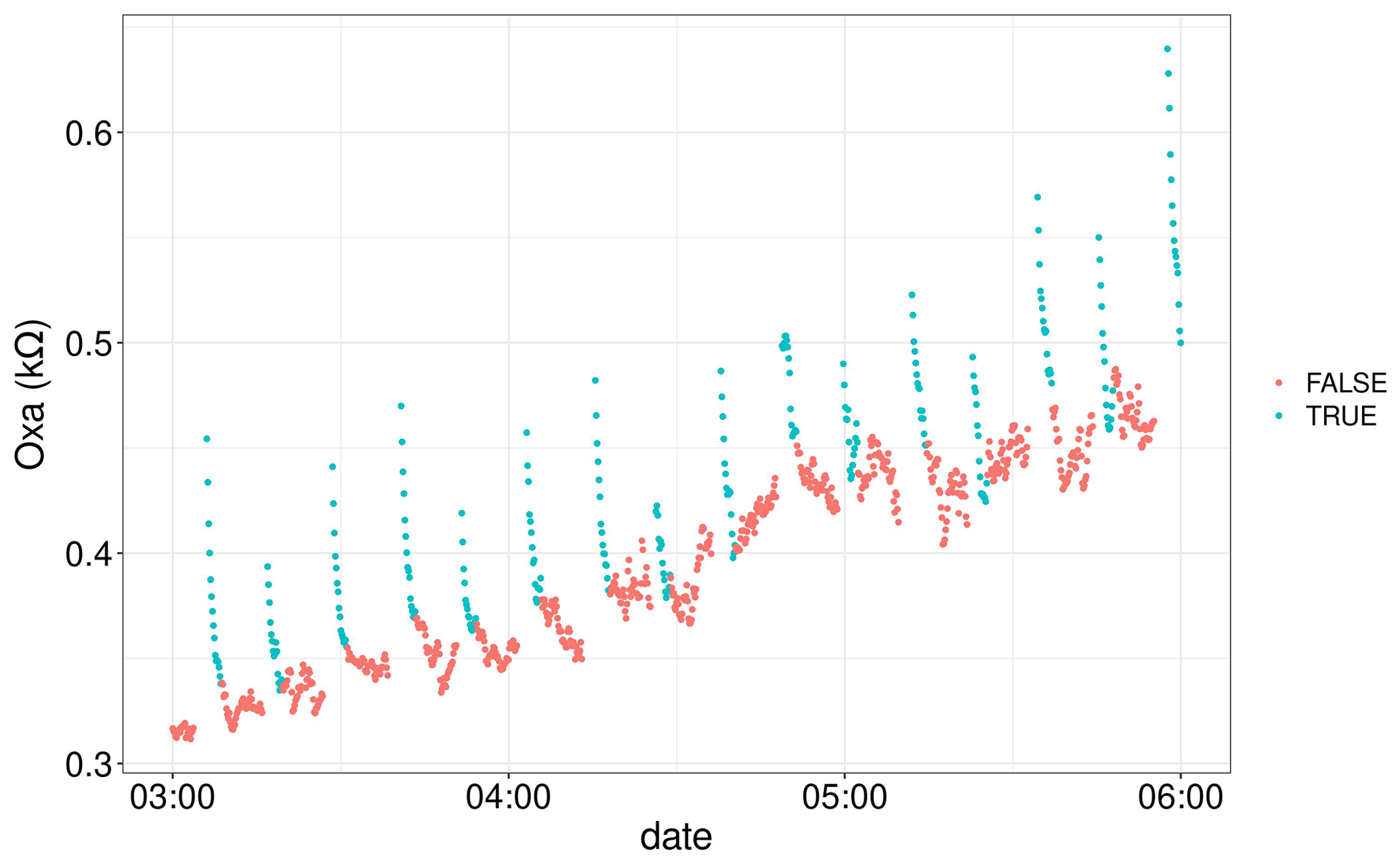
Figure 6 Example of outliers due to MOS warm-up following a GSM connection of the Zephyrs. A value of “TRUE” indicates the point was included in the 2.5 min MOS warm-up period.

Once the time-gap anomalies were removed from the Zephyr data, the outlier detection function was applied to the four Zephyr variables in original time resolution. As can be seen in Fig. 7, outliers were detected for the four Zephyr variables with a z-score threshold of 5 and a running mean of 360 data points (equivalent to 1 h of data). It is likely that these anomalous data points all result from brief technical failures within the instrument.

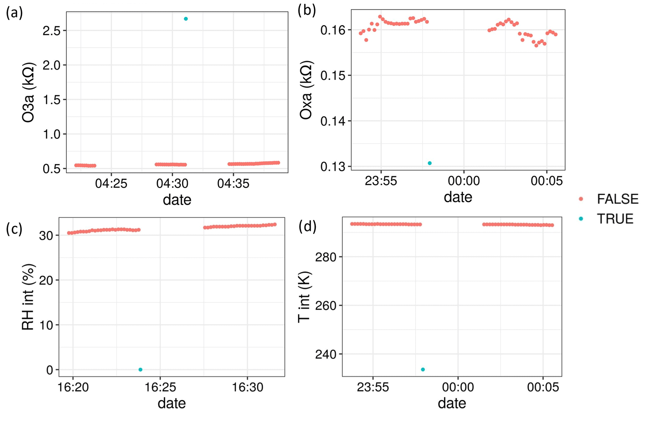
Figure 7 Examples of outliers detected on Zephyr s71 data using a z test with running mean for the SC. A value of “TRUE” means the point was deemed an outlier.

3.4.3 Step 3: flagging the data

Given that the data coverage from the second co-location encompassed most of the experimental data, only a few points during the experiment were flagged for being out of bounds of the second co-location set. As can be seen in Fig. 8a, only low NO₂ concentrations from the experimental set were flagged. The third co-location experienced a narrower range of NO₂ concentrations, as can be seen in Fig. 4 from Step 1. As such, more experimental data points of lower concentrations and some of high concentrations were flagged for this co-location (Fig. 8b). This shows the utility of comparing the results of Step 1 with the flags generated in Step 3.

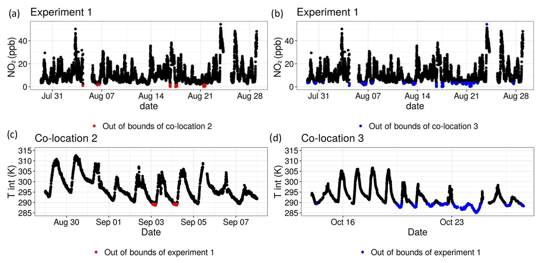
Figure 8 (a, b) Example time series plots of the experimental data with points out of bounds of the second and third co-locations flagged, respectively. (c) Time series plot of the second co-location with points flagged for being out of bounds of the experimental dataset. (d) Time series plot of the third co-location with points flagged for being out of bounds of the experimental dataset.

Similarly, the second co-location dataset received few flags, as most variables had comparable ranges to those of the experimental dataset. For example, only a few data points in which the internal Zephyr temperature dipped below ∼ 289 K were flagged (Fig. 8c). For the third co-location, which was conducted in colder conditions in October, far more data points were flagged (Fig. 8d). This indicated that a larger portion of the third co-location could be unsuitable for use in calibration. It also proved valuable for later analysis when analysing the final predicted concentrations of the model in Step 6.

3.4.4 Step 4: model selection

The results of the model selection process can be seen in Tables 2–5. For readability, these tables reflect a later stage in the process, after which a wide range of other models had already been tested and excluded on the basis of AIC and accuracy metrics. A combination of these metrics was used to designate the “best” models in which RMSE and R² received a higher priority than AIC. The most accurate MLR model for predicting NO₂ was determined to be one in which Oxa, O3a, RH, and T were included as single terms with interactions between all variables. The relationship between NO₂ and Oxa was determined to be logarithmic, whereas the relationship to T was determined to be inverse. This is in line with what would be expected in urban environments, as T can be seen as a proxy for insolation, which causes the photolysis of NO₂. For O₃ the most accurate MLR model had Oxa, O3a, RH, and T included as single terms with interactions. The relationship between Oxa and O₃ was also determined to be logarithmic. For both NO₂ and O₃, MLR models using ambient T and RH were consistently more accurate than those using internal T and RH.

Table 2 Results of the MLR model selection process for NO₂. The most accurate model is in bold. RMSE and MAE are in units of parts per billion.

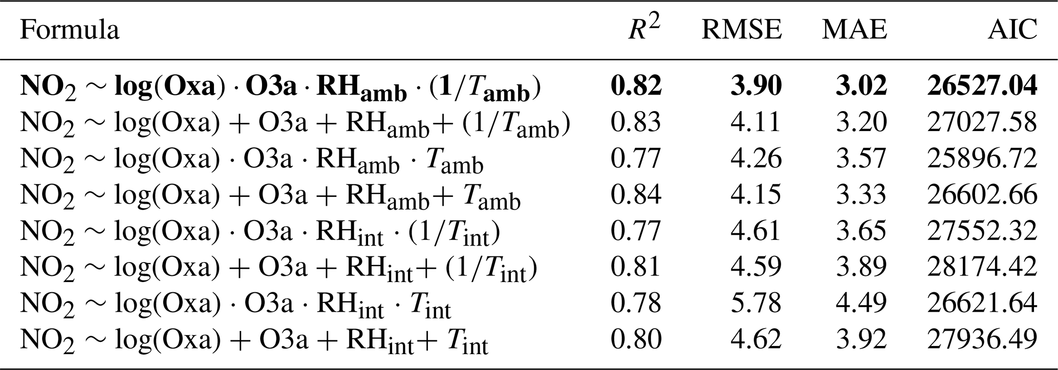
Table 3 Results of the MLR model selection process for O₃. The most accurate model is in bold. RMSE and MAE are in units of parts per billion.

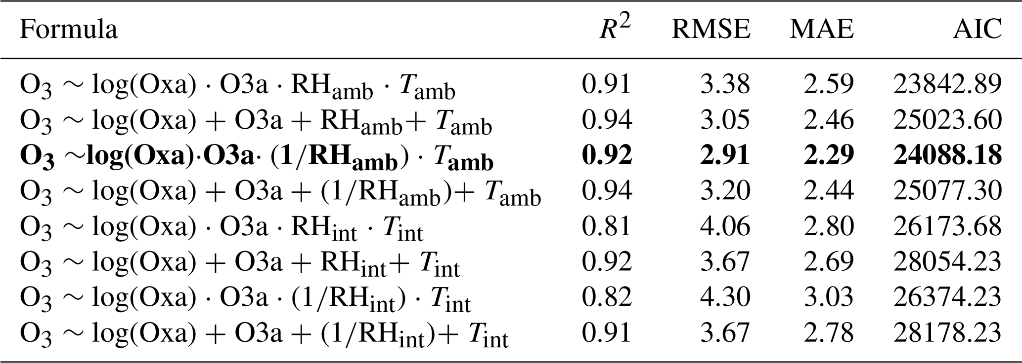
Table 4 Results of the RF model selection process for NO₂. Min.node.size and split rule were optimized in a previous step not shown here for brevity and are therefore constant. The most accurate model is in bold. RMSE and MAE are in units of parts per billion.

Table 5 Results of the RF model selection process for O₃. Min.node.size and split rule were optimized in a previous step not shown here for brevity and are therefore constant. The most accurate model is in bold. RMSE and MAE are in units of parts per billion.

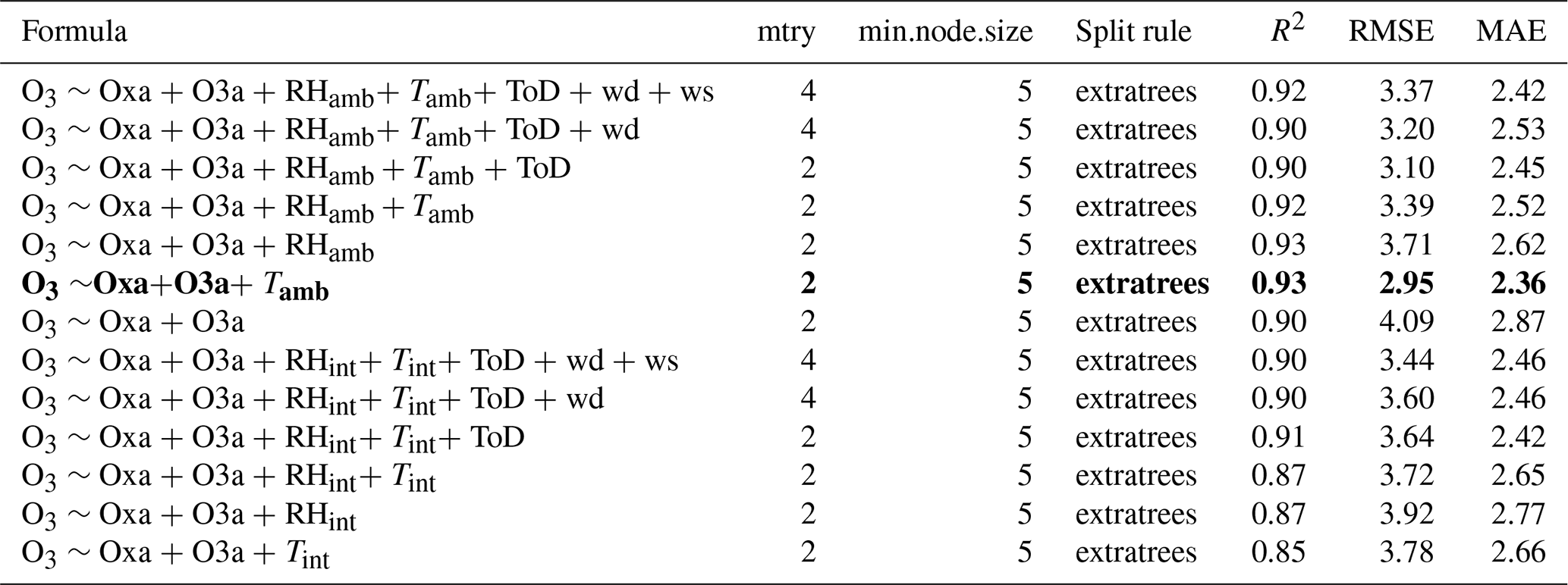
For random forest, the most accurate NO₂ model was determined to be one that included Oxa, O3a, ambient RH, and ambient T. The optimal mtry parameter was determined to be 4, with a minimum node size of 5. For predicting O₃ the results were similar to those of NO₂, except that ambient T replaced ambient RH. For both NO₂ and O₃ the use of ambient T and RH produced more accurate models. Overall, the RF models performed very similarly to the MLR models, with only slight differences in R² and RMSE.

3.4.5 Step 5: model validation

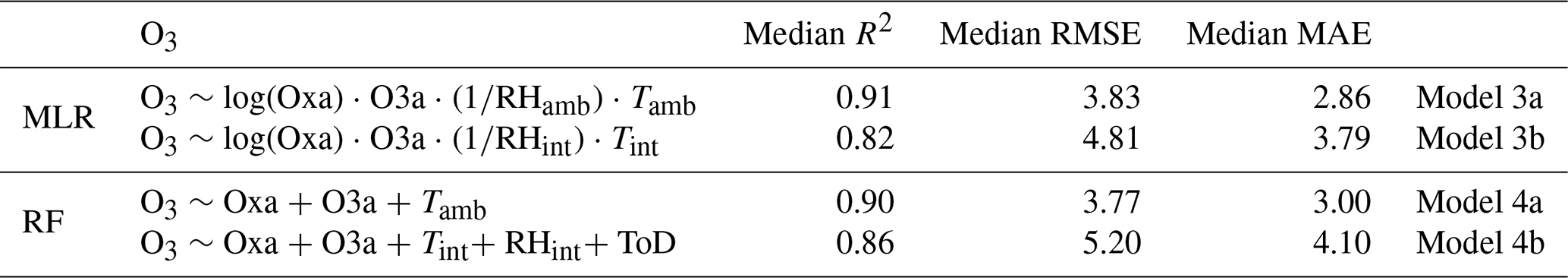
For MLR and RF, the R² and RMSE for each block were saved and plotted (Fig. 9a–d). As can be seen, the models using ambient T and RH for both O₃ and NO₂ remained relatively stable across all blocks. They consistently have a higher R² and a lower RMSE than the models trained with internal T and RH, for both NO₂ and for O₃. Conversely, the models trained with internal T and RH are much more volatile in terms of R² and RMSE, for both NO₂ and O₃. In addition, blocks 11, 12, and 13 show a marked decrease in R² and increase in RMSE across all models with internal T and RH. This trend was true for several models tested at this step, indicating that the internal T and RH were less stable for these blocks. Generally, the differences in RMSE between ambient and internal T and RH were more pronounced for NO₂ than for O₃. This is true across most blocks and indicates that the final concentrations should be predicted using ambient T and RH data instead of internal data. Tables 6 and 7 show the median R² and RMSE for all selected models for NO₂ and O₃, respectively. They reveal that MLR and RF models using ambient T and RH are similarly accurate at predicting NO₂ and O₃. The differences in accuracy are more pronounced for the models using internal T and RH.

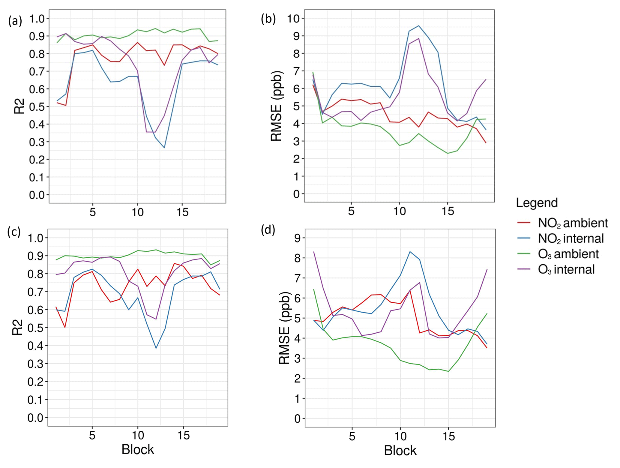
Figure 9 (a) R² and (b) RMSE over the 19 test blocks for the MLR models (1a, 1b, 3a, 3b). (c) R² and (d) RMSE over the 19 blocks for the RF models (2a, 2b, 4a, 4b).

Table 6 Median R² and RMSE across all test blocks of the best MLR and RF models using internal and ambient T and RH for NO₂. RMSE and MAE are reported in units of parts per billion.

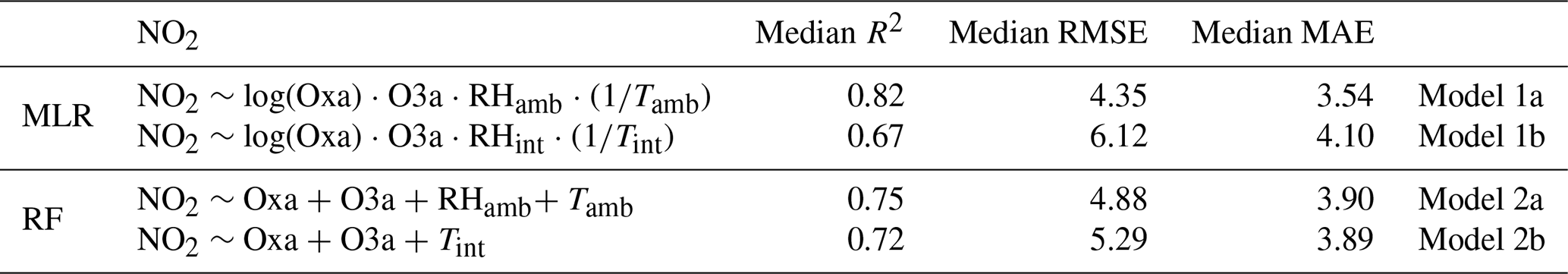
Table 7 Median R² and RMSE across all test blocks of the best MLR and RF models using internal and ambient T and RH for O₃. RMSE and MAE are reported in units of parts per billion.

Of all predictors included in the RF models, the MOS variable O3a had the highest VI for predicting both O₃ and NO₂ (Fig. 10a–d). The MOS variable Oxa was also of relative importance, usually as the second most important variable, with the exception of the O₃ models for which temperature (internal or ambient) was sometimes the second most important variable. Results from these graphs indicate that all variables should remain in the RF models.

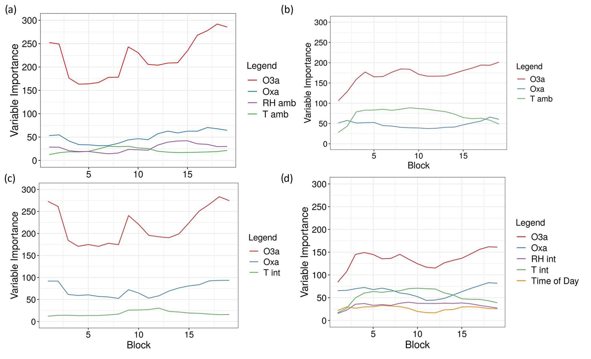
Figure 10 Variable importance over the 19 test blocks of (a) model 2a, (b) model 4a, (c) model 2b, and (d) model 4b.

3.4.6 Step 6: predicting final concentrations

Final concentrations predicted for NO₂ and O₃ using the MLR and RF models with both ambient and internal T and RH can be seen in Fig. 11. While the results indicated that ambient T and RH should be used, both are included here for further analysis beyond the seven-step methodology. For NO₂, the MLR models predict a much narrower range of concentrations and occasionally predict negative concentrations (Fig. 11a). The RF models tend to predict higher concentrations than MLR, have a wider range, and do not predict negative concentrations (Fig. 11b). For O₃, the differences between MLR and RF are less pronounced, with both capturing the diurnal cycle well (Fig. 11c–d). In all figures it can be seen that models using ambient T and RH consistently predict higher concentrations than those using internal T and RH. This indicates that there is a difference between predictions using Zephyr internal versus reference temperature and relative humidity sensors.

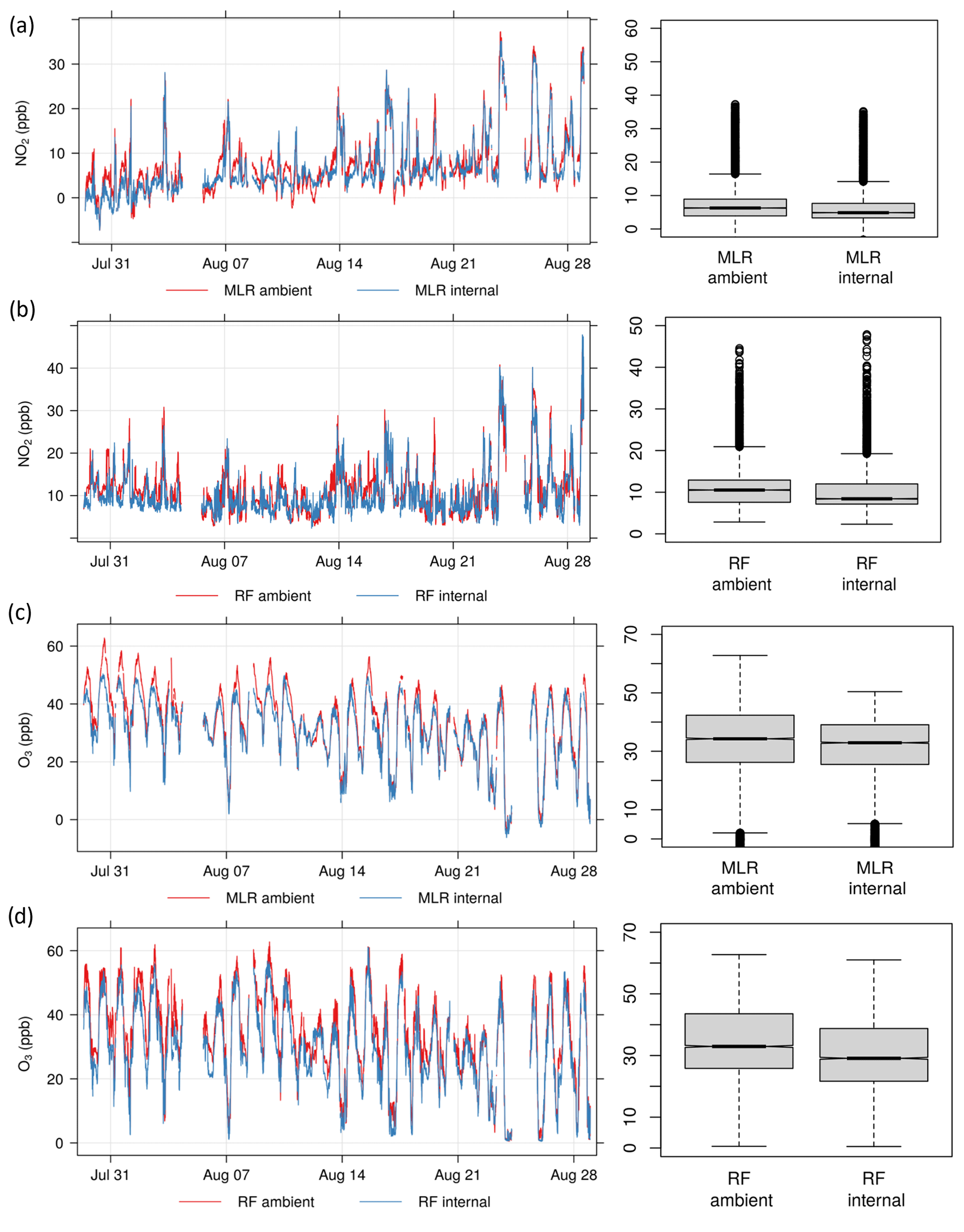
Figure 11 Time series plots and boxplots for Experiment 1 of (a) predicted NO₂ concentrations using the MLR model, (b) predicted NO₂ concentrations using the RF model, (c) predicted O₃ concentrations using the MLR model, and (d) predicted O₃ concentrations using the RF model. “Ambient” and “internal” refer to the use of ambient or internal T and RH data in each model.

3.4.7 Step 7: calculating predictive error

As can be seen in Fig. 12, smearing the reference data had minimal impact on the predictive accuracy of all models. This indicates that the uncertainty of the reference instruments did not impact the predictive accuracy of the models and can therefore in this case be ignored as a potential interference. Overall predictive error was then calculated as the reference error plus median MAE of each model across all blocks from the model validation step. The T-200 NO_x instrument has a measurement uncertainty of 0.5 % of the measurement above 50 ppb or an uncertainty of 0.2 ppb below 50 ppb. For the 2B Technologies ozone monitor, the uncertainty was larger, between 2 % of the measurement or 1 ppb. This can be seen in Fig. 13, which depicts the MLR and RF-predicted concentrations for Experiment 1, with shaded regions representing the uncertainty. The uncertainty of the RF and MLR models was fairly similar but was higher for NO₂ than for O₃. This reflects the findings from Steps 4–6 in which O₃ was predicted more accurately than NO₂ by both models. The standard error for MLR models was found to not reflect the realistic accuracy of the predicted concentrations in relation to actual concentrations, as it was found to be very low. The RF models calculated a more appropriate measure of standard error using the infinitesimal jackknife method (Wager et al., 2014), but for consistency with the MLR models, this measure was not used. The accuracy of the final models in predicting experimental data for which reference concentrations are not available for comparison is then best reflected by combining the uncertainty of the reference instruments with the median MAE of the test blocks during Step 5 (Tables 6 and 7).

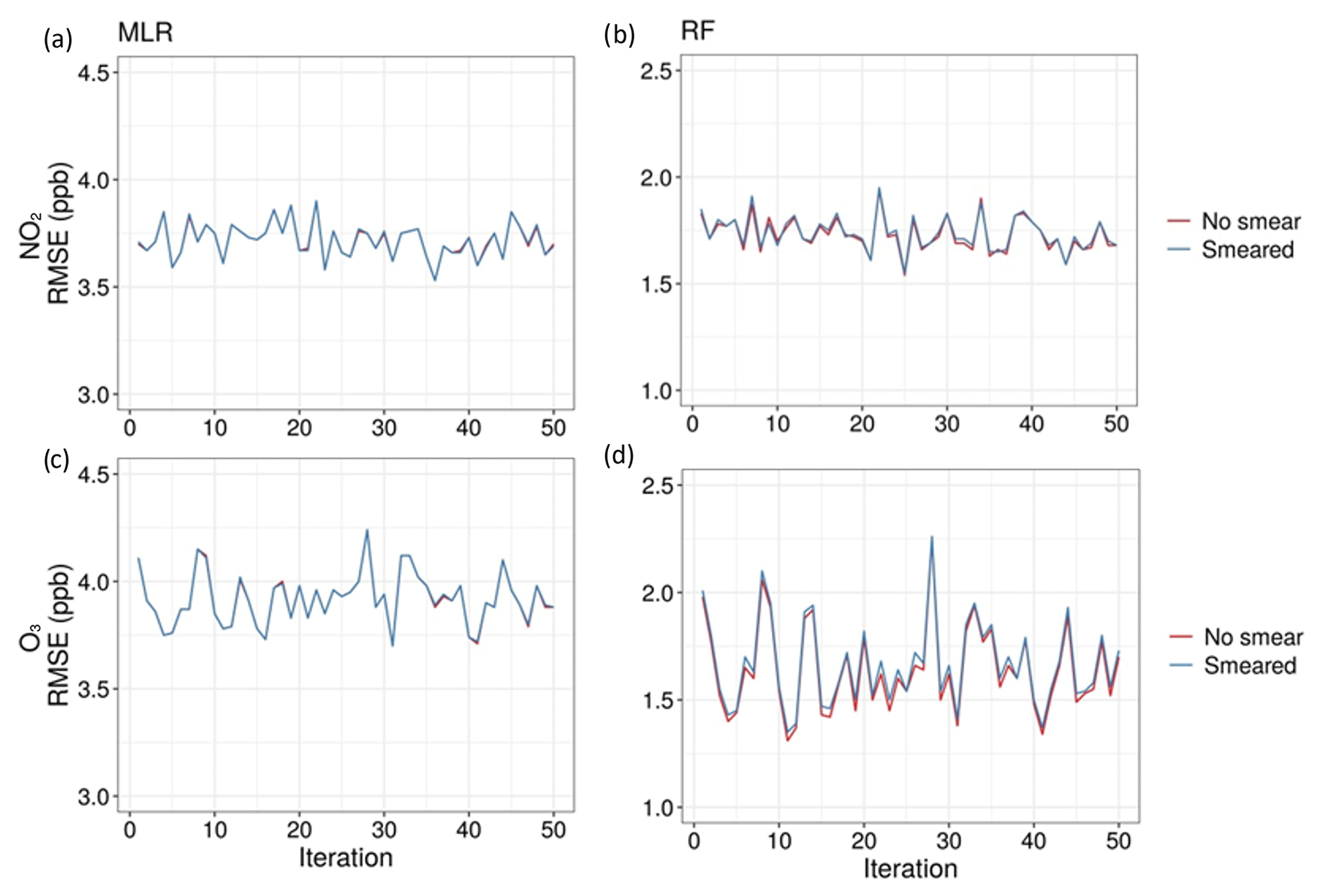
Figure 12 RMSE of models trained using smeared reference measurements versus actual reference measurements for (a) NO₂ with MLR, (b) NO₂ with RF, (c) O₃ with MLR, and (d) O₃ with RF.

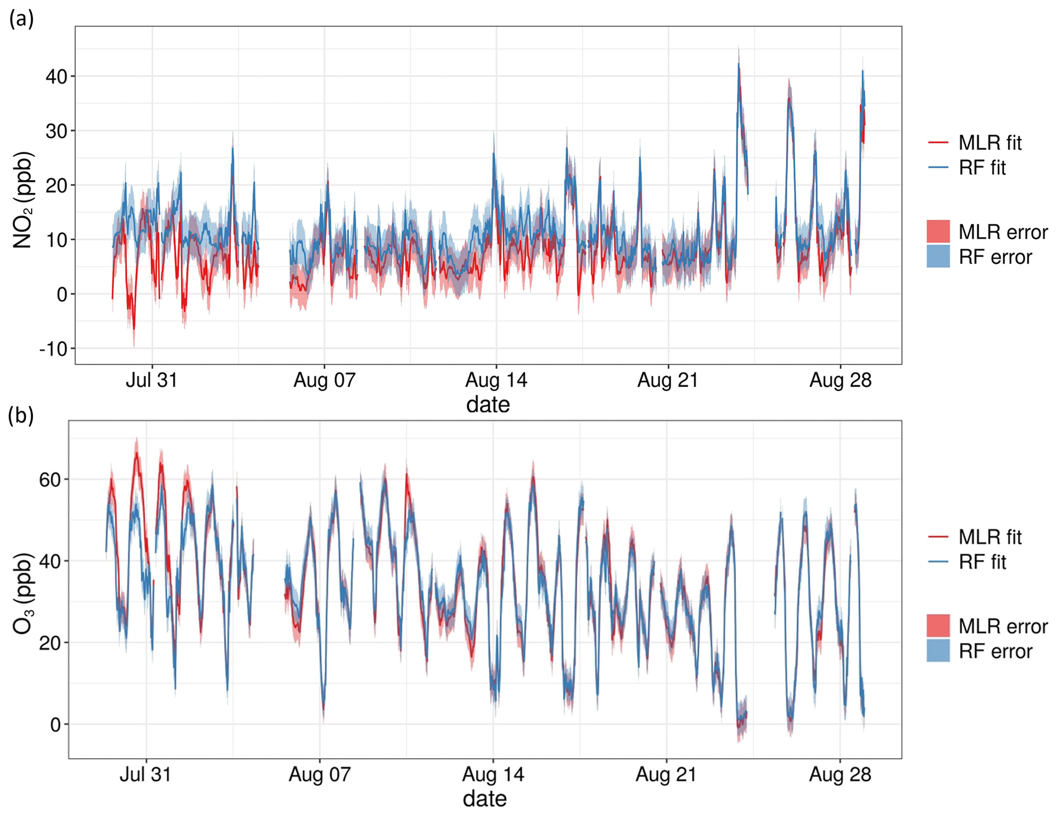
Figure 13 Time series plots of both MLR and RF predictions for Experiment 1 including the measurement uncertainty as shaded regions for (a) NO₂ and (b) O₃. Data were averaged to 30 min resolution.

3.5 Extra validation step

To further test the impact of using more representative training datasets, the final models identified in Steps 4 and 5 were trained with each co-location individually as well as with both combined. The predictive accuracy of these separate models was then compared using the experimental dataset for which reference NO₂ and O₃ measurements were available, as Zephyr s71 was co-located throughout the experiment. Additionally, these datasets were also tested with data points flagged in Step 3 removed to understand further influences on model accuracy. This extra validation allowed for better evaluation of the performance in predicting experimental concentrations of the MLR and RF models selected with the seven-step method. This is, however, atypical for field studies, as these sensor systems are intended to be deployed independently of reference instrumentation.

Table 8 shows the results of training these various models for NO₂. The most accurate model at predicting experimental concentrations was the RF model using internal T and trained with data only from co-location 2. The same model trained with all available co-location data was slightly more inaccurate. Co-location 3 was the least accurate of the training subsets, reiterating findings from Step 1. For the MLR models, this dip in accuracy when exclusively using co-location 3 as the training set was most pronounced, as can be seen in Table 8 and Fig. 14g–h. When filtering out flagged data points, most NO₂ models improved slightly in predictive accuracy. This was most pronounced for those using co-location 3 as a training set, which improved substantially in terms of R². This alludes largely to the impact of seasonal changes on co-location 3, which experienced different meteorological and pollution conditions than were present during experiment 1. While results show that this co-location was not useful for accurate prediction, it is likely that it would have been more relevant for prediction on experiment 2, during which the environmental conditions were more comparable. Similarly, co-location 1 would likely have been more valuable for prediction with experiment 1 than with experiment 2. However, due to the loss of data from s71, this could not be assessed more closely in this study.

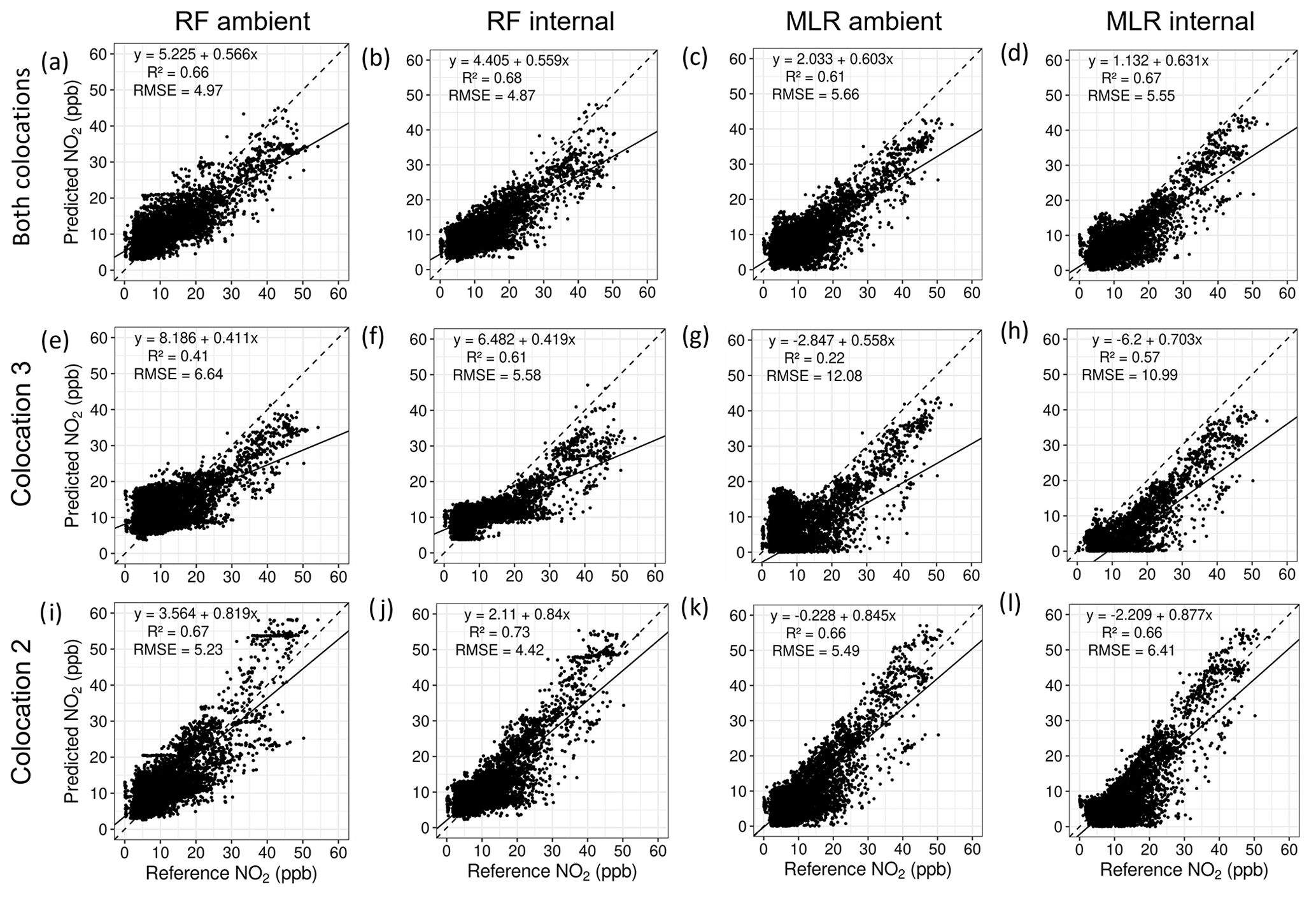
Figure 14 Scatter plots of predicted NO₂ versus reference NO₂ concentrations for the experimental data using MLR and RF models trained with co-location 2 (i–l), co-location 3 (e–h), and both combined (a–d). All concentrations are reported in parts per billion.

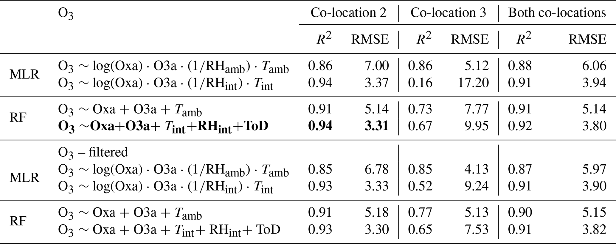
For O₃, the most accurate model was the RF model using internal T and RH and trained exclusively using data from co-location 2, though the MLR internal model for the same co-location was of comparable accuracy. The RMSE for this model was substantially lower than the one trained using ambient T and RH. With the MLR models, this difference in predictive accuracy between models trained with internal and ambient T and RH was much greater, again favouring the internal models. Co-location 3 was highly inaccurate at predicting experimental data, further reiterating findings from Step 1 that indicated the unsuitability of this co-location for use in predicting final concentrations. Panels e–f in Fig. 15 clearly depict the boundaries for predictions with RF models when the training data are unsuitable, as is the case with co-location 3. This is a fundamental flaw of RF models as they cannot predict outside the bounds of the data they are trained with. Filtering out the points flagged in Step 3 did not improve the predictive accuracy of models trained exclusively with co-location 2, but it substantially improved those trained with co-location 3, especially those using internal T and RH.

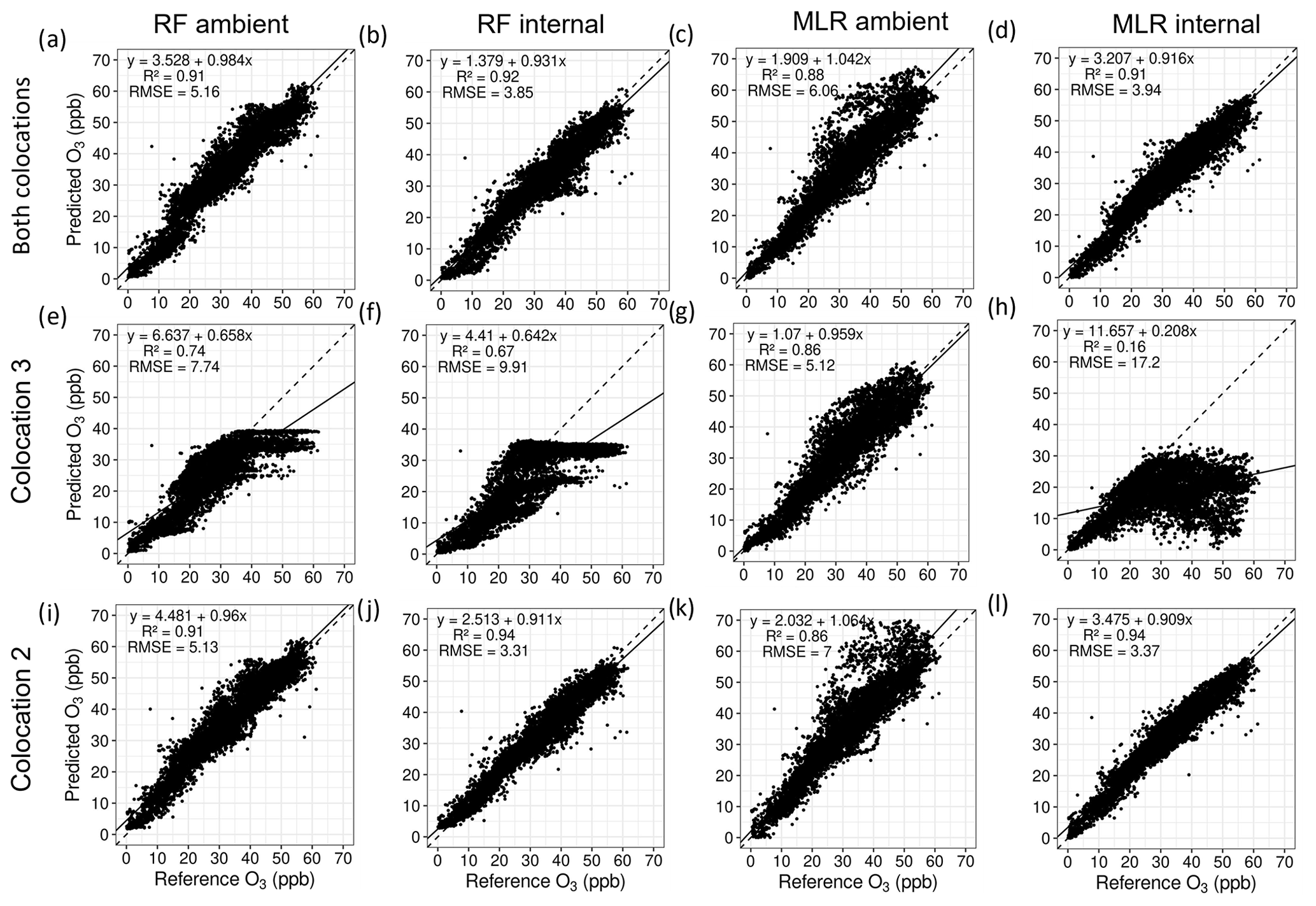
Figure 15 Scatter plots of predicted O₃ versus reference O₃ concentrations for the experimental data using MLR and RF models trained with co-location 2 (i–l), co-location 3 (e–h), and both combined (a–d). All concentrations are reported in parts per billion.

Table 8 Results of RF and MLR models for NO₂ trained with co-location 2, co-location 3, or a combination of both when tested on the comparison experimental dataset. In the lower half of the table, the models are trained with the same datasets but are tested on the experimental dataset with data points outside the ranges of each training dataset filtered out. The most accurate model is in bold.

Table 9 Results of RF and MLR models for O₃ trained with co-location 2, co-location 3, or a combination of both when tested on the comparison experimental dataset. In the lower half of the table, the models are trained with the same datasets but are tested on the experimental dataset with data points outside the ranges of each training dataset filtered out. The most accurate model is in bold.

4 Discussion

The results of this study have several implications for the field of low-cost sensors. In line with other research, this study found that MLR and RF were similarly accurate in predicting experimental concentrations of NO₂ and O₃ (Karagulian et al., 2019), though the differences in accuracy between MLR and RF were more pronounced for O₃ than for NO₂. In fact, it was found that RF was the better predictor of both O₃ and NO₂ concentrations when evaluated with the longer experimental dataset, albeit only slightly. This contrasts with findings from the model selection and validation process, as the MLR models were consistently more accurate at predicting subsets of the co-location data. What this indicates is that models found to be more accurate during “calibration” may have differing model performance when assessed with a “comparison” dataset, in this case the experimental dataset that was co-located throughout for one sensor. This is a result that has been found previously, where the R² is lower for comparison datasets than for calibration (Karagulian et al., 2019). If RF, MLR, or other ML techniques are selected for their accuracy when predicting on calibration data and are not tested on comparison data, it may well be that the performance does not hold for new experimental data. Given the similarity between RF and MLR in predicting NO₂ and O₃ found in this study, as well as in the literature, either method can be used. However, as MLR is simpler to implement than most ML techniques and has fewer parameters that need to be optimized, and the model calculations are well understood, unlike the black-box calculations of RF and most ML techniques, this should be the preferred option to achieve greater model transparency and control.

Further important to the proper evaluation of model accuracy is the reporting of multiple metrics such as RMSE and MAE, in addition to R². It is quite clear from Tables 8 and 9 that R² is not the best metric with which to measure predictive accuracy of calibration models. Models trained with co-location 3 exclusively to predict O₃, for example, had an R² greater than 0.70, which is acceptable agreement. Those same models, however, had an RMSE of >7 ppb, which is much more inaccurate than an R² of 0.70 alone would reveal. As another example, the same models trained exclusively with co-location 2 for O₃ (Table 9) had an R² between 0.86 and 0.94 but had a wide range of RMSE between 3.30–7.00 ppb. It is therefore crucial that multiple performance metrics are used to evaluate calibration models before final decisions are made on their suitability. At a minimum, R² and RMSE should be reported.

Multicollinearity is an issue common not only to MLR, but also to small sensor systems, which often have multiple LCSs measuring the same or similar species with heavily auto-correlated data. While uncommonly addressed in the literature, except for a few studies mentioning its influence on MLR models (Bigi et al., 2018; Hagan et al., 2018; Masiol et al., 2018), the solution, as presented in Steps 4 and 5, is relatively straightforward. To ensure that the predictor variables included in the final model are, in fact, explanatory, the model should be repeatedly validated using bootstrapped samples. To deal with autocorrelation, this validation should be done using continuous blocks and not with random sampling. Including these steps in the model-building process is simple and should be considered best practice.

Further underlining the importance of repeated validation is the variation in results when using ambient or internal T and RH. While the inclusion of ambient meteorological data led to more accurate models during calibration, this did not hold for the comparison dataset. Instead, for the prediction of both NO₂ and O₃, it was internal T and RH data that led to more accurate prediction. This indicates that for the prediction of NO₂ and O₃ concentrations with EarthSense Zephyrs, not only are the internal T and RH sensors acceptable for use in predictive models, but they are also likely more representative of normal operating conditions. Given that the MOSs radiate large amounts of heat, the conditions inside the Zephyrs are significantly different than ambient conditions. As such, the internal T and RH sensors likely better represent the exact environmental conditions under which species are adsorbing to the MOSs. However, given that models using ambient data were more accurate during the validation step and significant differences between predictions of models trained with internal vs. ambient T and RH were identified, these results require closer inspection, which should be the subject of future research.

The final results also reveal the value of pre-processing the data in Steps 1–3. It became clear by looking at the distribution of the co-location datasets in Step 1 that co-location 3 might be unsuitable for use in predicting the experimental concentrations. These data were then flagged in Step 3. While the models trained exclusively with co-location 3 were substantially less accurate than those using data from co-location 2, their accuracy increased when flagged experimental data points outside the range were removed. In essence, the third co-location was useful for predicting experimental data within its range of conditions but very inaccurate for those outside of that range. Co-location 2, on the other hand, was identified as being well-suited for prediction in Step 1 and received few flagged points in Step 3. Final results indicate that MLR and RF models trained with co-location 2 perform better than those trained with co-location 3, for both NO₂ and O₃. Combining the two co-locations did not improve the predictive accuracy for NO₂ or O₃, when compared with the more-suitable second co-location (Tables 8 and 9). As such, training calibration models with co-location 2 exclusively would have been correctly justified using evidence from Step 1. What is evident from this analysis is that ensuring quality of training data used in calibration is crucial to accurate prediction. Incorporating quality control into the calibration methodology is therefore an important best practice.

Finally, LCS data should be reported with associated error values. While we discussed RMSE in the context of model fit and validation, as well as a method for evaluating whether reference instrument accuracy affects the model output, error values should be reported not just in the assessment of the LCSs themselves, but also with some form of representative error associated with the reported concentration data. Our recommendation is to combine the uncertainty of the reference instruments with the median MAE across blocks from the model validation step. As can be seen in Tables 8 and 9, the RMSE of predictions tested with the comparison experimental dataset are quite similar to the median RMSE values in Tables 6 and 7. This indicates that using median error from the model validation step is quite representative of the LCS uncertainty. However, over longer measurement campaigns, this should be repeatedly tested and validated with additional co-location training sets, so as to account for sensor drift, deteriorating functionality, and varying meteorological conditions.

5 Conclusions

While many details of this methodology are already well-known, they are often overlooked or go unreported in published literature. In most cases not all aspects are included. As a result, many studies assessing pairwise calibration methodologies for low-cost sensors cannot be compared. In the absence of calibration standards for these technologies in a field that continues to diversify and grow, researchers must start to consolidate around an agreed-upon set of best practices. This study has highlighted several of them. First, details on model selection, validation, and tuning must be reported if researchers are to be able to effectively compare results across studies. If models are not rigorously tested for suitability using standardized methods, especially with “black-box” machine-learning techniques, then their comparison will remain challenging at best. Second, models should be validated not only on the calibration dataset but also on a separate comparison dataset, if possible. All validation should be done using R² and RMSE, at a minimum. This will provide greater insight into the suitability of selected models for prediction on experimental data as well as better comparability across studies. Third, pre-processing the data, including visual inspection, outlier removal, and data-flagging, is an integral part of an effective calibration methodology. Understanding the quality and distribution of available data is important to identifying problems and solutions encountered during calibration.

Last, it is clear that a standardized methodology for the calibration of low-cost sensors is needed if they are to be incorporated into air quality monitoring programmes and contribute new insights to the field of atmospheric chemistry. This seven-step methodology seeks to fill a gap in the literature up until now left largely unreported. In addition, this methodology, complete with relevant R code, is the first to be completely transparent and open access. This is a valuable contribution to a young but rapidly growing body of literature surrounding low-cost sensors. With this work, we hope to begin unravelling the black box of sensor calibration.