the Creative Commons Attribution 4.0 License.
the Creative Commons Attribution 4.0 License.
 | 01 Dec 2021
Use of thermal signal for the investigation of near-surface turbulence
Organised motion of air in the roughness sublayer of the atmosphere was investigated using novel temperature sensing and data science methods. Despite accuracy drawbacks, current fibre-optic distributed temperature sensing (DTS) and thermal imaging (TIR) instruments offer frequent, moderately precise and highly localised observations of thermal signal in a domain geometry suitable for micrometeorological applications near the surface. The goal of this study was to combine DTS and TIR for the investigation of temperature and wind field statistics. Horizontal and vertical cross-sections allowed a tomographic investigation of the spanwise and streamwise evolution of organised motion, opening avenues for analysis without assumptions on scale relationships. Events in the temperature signal on the order of seconds to minutes could be identified, localised, and classified using signal decomposition and machine learning techniques. However, small-scale turbulence patterns at the surface appeared difficult to resolve due to the heterogeneity of the thermal properties of the vegetation canopy, which are not immediately evident visually. The results highlight a need for physics-aware data science techniques that treat scale and shape of temperature structures in combination, rather than as separate features.
- Article
(10627 KB) - Full-text XML
- BibTeX
- EndNote


Available methods to determine energy and scalar fluxes from the terrestrial land surface are relatively imprecise due to a multiscale of irregularities in the land surface and the turbulent transport mechanisms (Brutsaert, 1998). The most broadly adopted micrometeorological methods for quantification of surface exchange fluxes take an integrative approach to observations in the atmospheric surface layer (ASL) and have become a crucial component in global Earth system assessments on climate change mitigation (Foken, 2006). On that account, questions have been asked about additional details contained in such data (e.g. Knauer et al., 2017; Klosterhalfen et al., 2019; Clement and Moncrieff, 2019), but also, more pressingly, what we are missing outside the applicable range of the methodology and assumptions (Mahrt, 2010; Bou-Zeid et al., 2020).
The complex relationship between the scale and heterogeneity of a source area and observations of turbulence and temperature (and humidity) in the ASL has been broadly recognised (Garratt, 1980; Schmid, 1994; Raupach and Finnigan, 1995; Mahrt, 1996; Sun et al., 1999; Li et al., 2012; Patton et al., 2016) in decades of work that contributed to the best-practice guidelines for the eddy-covariance technique (Lee et al., 2005; Aubinet et al., 2012). The atmosphere, the surface and the plant microclimate are in direct exchange in the so-called roughness sublayer, the internal ASL layer below the inertial sublayer (Raupach, 1979; Garratt, 1980; Stull, 1988). Finnigan (2000) provides a detailed review on aspects of turbulence within the roughness sublayer (RSL), where individual roughness elements modulate the flow in a three-dimensional and inhomogeneous way. The correlation between the statistics of turbulence, air temperature and skin temperature of vegetation has been investigated using single-point observations as well as spatial data (Finnigan, 1979; Paw U et al., 1992; Shaw et al., 1995; Katul et al., 1998), highlighting the presence of organised structures in the RSL in accordance with insights from laboratory experiments on near-wall fluid dynamics (Kline et al., 1967). Coherency of eddies has been observed in profiles within the RSL from vector and scalar data, such as temperature (Antonia et al., 1979; Williams and Hacker, 1992). Many near-surface turbulence studies adopt Taylor's hypothesis (frozen convection) to translate wave numbers to length scales, but it could be questioned if and when the underlying assumptions hold, particularly for non-ideal conditions (stationarity, ergodicity, homogeneity; see, e.g. Higgins et al., 2013).
A way to avoid making such assumptions would be to observe turbulence features explicitly in space and time. Dense geometrically distributed observations of air and surface temperature in combination with the wind field have not been explored in great detail outside a wind tunnel, mostly because methods were not available or because the costs would be prohibitive. However, novel opto-electronic technologies may bring a needed change.
The availability of spatial surface temperature observations has improved with advancements in spectral imaging. Thermal infrared imaging (TIR) instruments observe long-wavelength infrared light from which a surface brightness temperature (Tb) can be derived. TIR instruments have proven to be sufficiently sensitive, as demonstrated in recent studies on spatial temperature fluctuations (Christen et al., 2011; Katurji and Zawar-Reza, 2016), planar flow fields (Abram et al., 2013; Inagaki et al., 2013; Burns and Chemel, 2014) and partitioning of energy fluxes (e.g. Kustas and Anderson, 2009). It should be noted that the sensitivity of TIR to measure Tb is affected by thermal signal other than the surface skin temperature. The quantification of Tb outside a controlled laboratory environment is a challenge, in and of itself; there are many possible sources of interference in thermal imaging, which in a controlled laboratory environment can be anticipated and corrected for. Parameters that affect the observation of Tb include external influences between the camera sensor and the object, variation in thermal admittance, thermal reflections, moisture and humidity (Vollmer and Möllmann, 2010; Jones, 1999).
Distributed temperature sensing (DTS) provides highly localised temperature observations along optical (silica) fibre (Dakin et al., 1985), making it a tool for spatial environmental sensing (Selker et al., 2006; Tyler et al., 2009). The optical fibre is usually packaged inside a cable for durability and to help minimise attenuation due to (micro)bending. The cable jacket adds surface and volume, making the measurement more susceptible to the local energy balance terms (Thomas et al., 2012; de Jong et al., 2015). Hence, micrometeorological studies with DTS have primarily been demonstrated for conditions of nocturnal darkness (Keller et al., 2011; Thomas et al., 2012; Zeeman et al., 2015) or, after adjustments, taking advantage of a differentiating thermal signal governed by wind, evaporation or shading of sunlight (Petrides et al., 2011; Euser et al., 2014; Sayde et al., 2015; Lapo et al., 2020; Schilperoort et al., 2018; van Ramshorst et al., 2020). Fibre-optic cables can be deployed to form a mesh of horizontal and vertical profiles in complex geometries from the ground up.
The goal of this study was to combine DTS and TIR for the investigation of temperature and wind field statistics near a vegetation surface. These novel methods are moderately precise but constrained in accuracy for observation of air and surface temperature. However, both DTS and TIR promise geometrically dense thermal information that could complement single-point observations using well-known sensing technique, such as ultrasonic anemometry for wind and metal wire resistance for temperature. The combined granularity may allow us to revisit the investigation of scale and structure in the roughness sublayer in more detail. The examination of multi-dimensional data has taken flight with the availability of novel statistics and machine learning tools, which will also be addressed.
The study was conducted at the DE-Fen station, Fendt, Peissenberg, Germany, which is a TERerstrial ENvironment Observatories (TERENO) and Integrated Carbon Observation System (ICOS) core site (Zacharias et al., 2011; Zeeman et al., 2017; Kiese et al., 2018). The site is a permanent grassland situated in a shallow valley bordered to the west by a steep, forested slope towards a plateau at approximately 150 m higher elevation (Fig. 1). During intensive field campaigns at DE-Fen, additional experiments were conducted for the investigation of scale interactions between the atmospheric boundary layer and the surface, as well as validation of measurement techniques (ScaleX; https://scalex.imk-ifu.kit.edu, last access: 17 December 2020; Wolf et al., 2017). The experiment took place during the ScaleX 2016 campaign in June–August 2016, but we focus here on the period 18–22 July 2016. These days included a typical summer warm-up phase with mostly clear-sky conditions and calm nights but with limited activity by uncrewed aerial vehicles (UAVs) perturbing the air by downwash and frequent transit through the area.
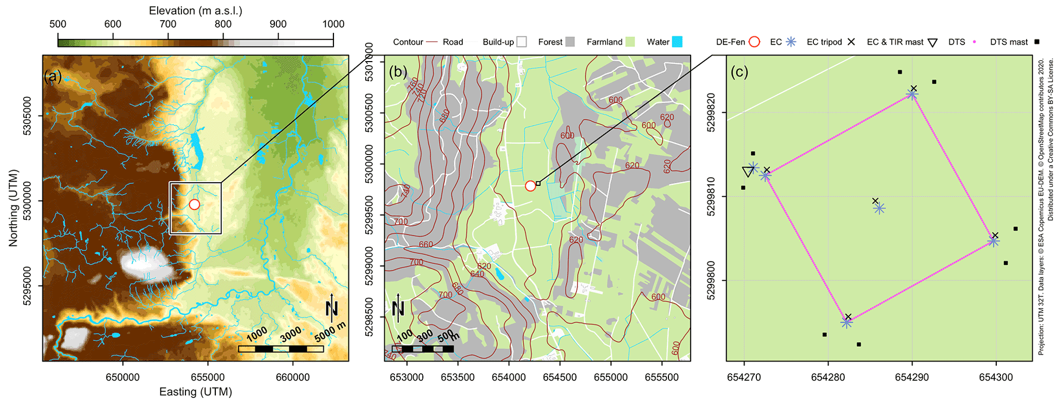
Figure 1The location of the study site with aspects of (a) topography and runoff, (b) land use and (c) the sensor network setup. Data layers: © ESA Copernicus EU-DEM. © OpenStreetMap contributors 2020. Distributed under a Creative Commons BY-SA License.
2.1 Ultrasonic anemometer (EC) network
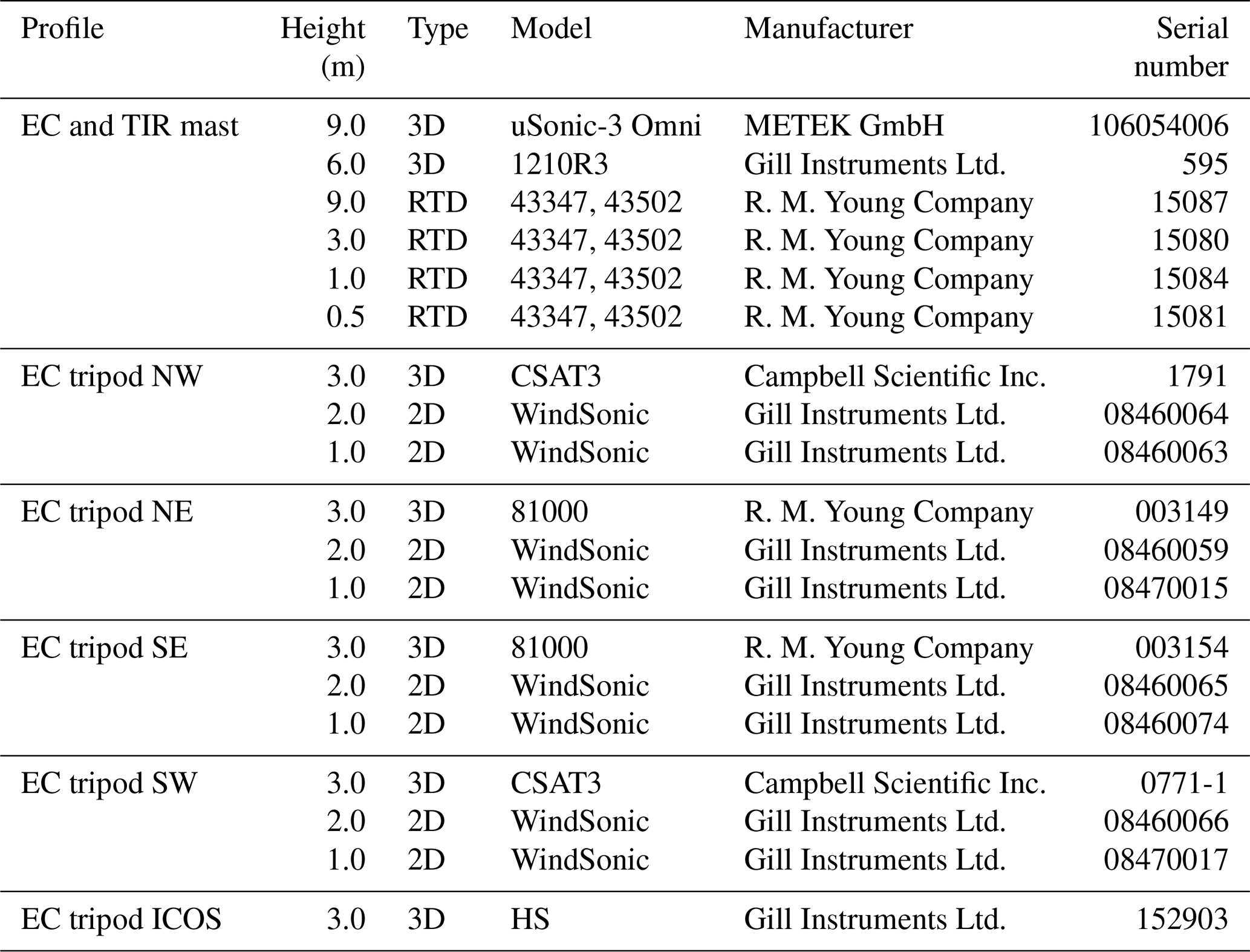
A network of wind sensors was deployed, comprising profiles of three-axis (3D) and two-axis (2D) ultrasonic anemometers on a guyed lattice mast and four tripods (Figs. 1c, 2; Table 1). The EC network was placed approximately 60 m east of the micrometeorological station of DE-Fen. The sensors were cross-calibrated prior to the experiment (Mauder and Zeeman, 2018). An additional EC station (ICOS; EC with trace gas analysers) was temporarily placed at the centre of the sensor network (Figs. 1c, 2).
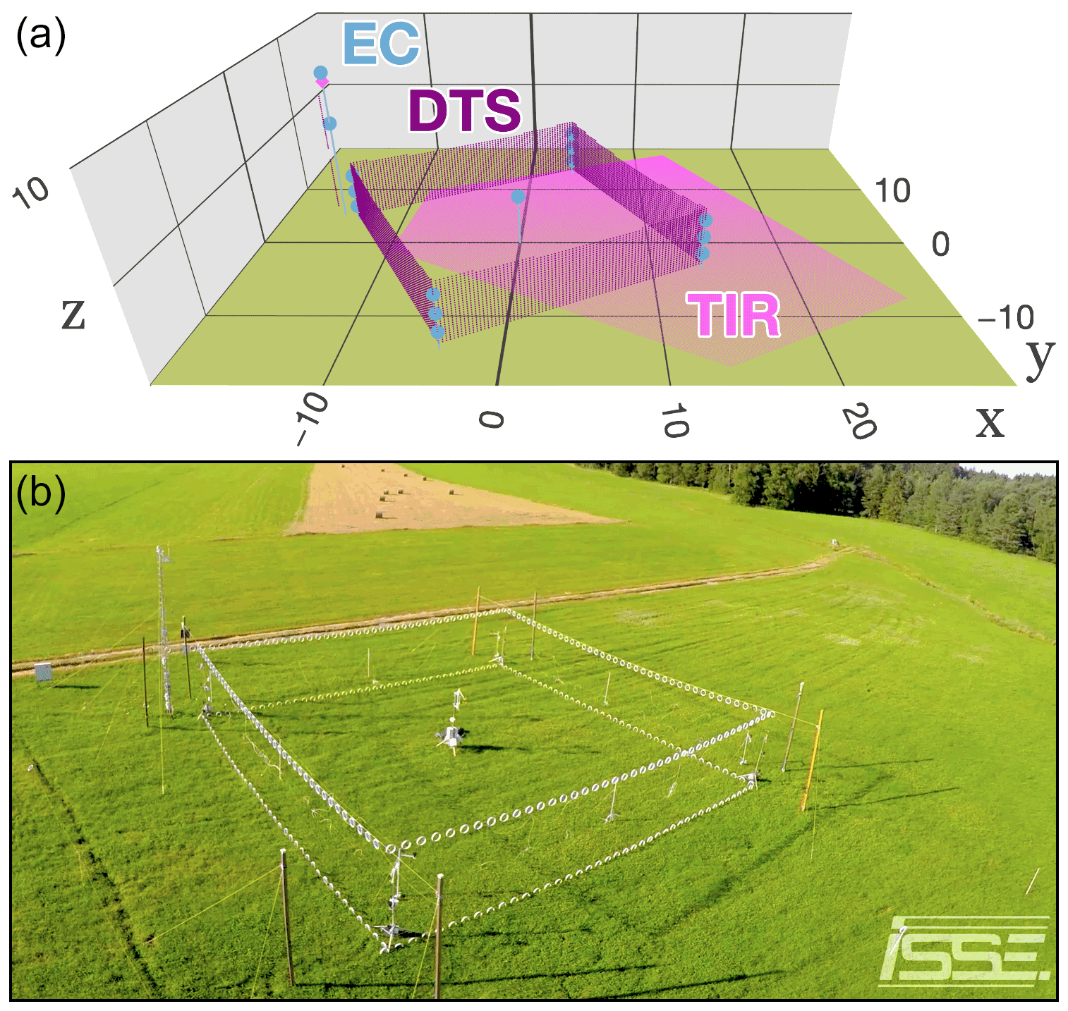
Figure 2Overview of the setup in (a) schematic perspective and (b) a bird's-eye view from the south. Still image has been modified from an aerial video by Martin Schörner (24 July 2016, ISSE/University of Augsburg).
Table 1Overview of profile instruments. The two-axis and three-axis ultrasonic anemometer are referred to as 2D and 3D, respectively.
2.2 Distributed temperature sensing (DTS)
The DTS setup consisted of a high-resolution instrument, custom fibre-optic cable and a calibration setup. The DTS instrument was configured to measure at 1 Hz and 0.15 m range gate intervals up to 1890 m (model Ultima-HS; Silixa Ltd., Hertfordshire, UK). The fibre-optic cable consisted of a bend-optimised optical fibre (Giga-Link communications type; 125 µm with 50 µm core), buffered with aramid fabric (Kevlar) in a white plastic jacket (900 µm outer diameter; AFL Telecommunications, Spartanburg, SC, USA). Both ends of the fibre-optic cable were connected to separate channels on the DTS instrument for measurement in both directions (Hausner et al., 2011). The configuration allowed two profiles along the lattice mast up to 8 m above ground and 316 profiles suspended in the air up to 4.5 m above ground. The latter were spatially configured to form the sides of a box of m [], or four planes of 80 vertical profiles in 0.25 m intervals, with EC profiles placed at each corner (Figs. 1c and 2). The dimensions were chosen as a trade-off between DTS range limitations, instrument spatial resolution and measures to limit systematic shading of direct solar radiation or wind by DTS and EC support structures. The effective thermal sensitivity is dependent on the instrument, the deployed cable geometry and the location along the fibre, which previously was estimated to be 0.5 K or better (Zeeman et al., 2015, see Appendix A3.1).
2.3 Thermal infrared imaging (TIR)
A thermal infrared imaging system was installed inside a weather-proof camera housing at 8.5 m above ground (8–14 µm spectral range, 40 mK thermal sensitivity, field of view and 382×288 pixels optical resolution; model PI 640, Optris GmbH, Berlin, Germany). The spectroscopic data were recorded at 2 Hz between 00 and 53′ in the hour with automatic self-calibration each 9 s.
2.4 Data integration
Each EC, DTS and TIR record was stored with an accurate time stamp and locations were georeferenced in post-processing. The calibration and georeference details are provided in Appendix A. The physical meaning of the EC-, DTS- and TIR-derived temperature measurements must be considered. Until that is fully explained, or until we assure the values match the expectation in atmospheric research, we should discern the nomenclatures from air temperature (Ta) or surface temperature (Ts). DTS can be used to measure temperature of air, but we denote it as “cable” temperature (Tc) below, in order to distinguish it from radiation-shielded and fan-aspirated sensing standards used for air temperature in micrometeorology. Following similar argumentation, Tb and Tv are differentiated here as surface brightness temperature and temperature from the speed of sound (or acoustic virtual temperature), respectively. The use of the EC-based Tv is common in micrometeorological studies, once noise and calibration have been handled with care (Mauder and Zeeman, 2018). Additional air temperature measurements were made using resistance temperature devices in fan-aspirated enclosures (Table 1; Appendix A).
2.5 Design considerations
As mentioned above, the setup was not a stand-alone experiment. The design was intended to support studies on atmospheric processes dedicated to empirical data and in combination with fluid dynamics models. Other experiments were conceptualised to use the setup, as part of cooperative research during the experimental campaign (ScaleX; see, e.g. https://scalex.imk-ifu.kit.edu, Brosy et al., 2017; Brenner et al., 2018; Mauder and Zeeman, 2018; Zhao et al., 2018; Ibraim et al., 2019; Hald et al., 2019; Zeeman et al., 2019; Kunz et al., 2020). Applications include the investigation of coherent structures, advection processes and conditional sampling methodology.
The placement of the wind sensors on the corners and at the centre of the setup was intended to facilitate the determination of a representative wind vector at the walls of the DTS array. It was thought that placing tripods at the centre of a wall would result in more uncertainty. The number and heights of the EC profiles were limited by available hardware at the time. Ideally, only three-axis sonic anemometers would be used. The dimensions and shape of the DTS array were primarily limited by the maximum range of the DTS instrument model, which can support up to 1.8 km of optical fibre per channel. The DTS profile height was extended to reach sufficiently above the sonic anemometers at 3 m. Small-scale disturbance in the wake of the DTS support structure was possible. The distance from the DTS masts to the EC profiles (on tripods) and DTS profiles was 3 m. The DTS masts had a diameter of 0.1 m. Increasing the distance would have required for the suspension cable to be mounted higher and with larger tension force to keep the steel cable straight. This could not safely be realised during the deployment. In an initial design, the guyed mast would be taller and placed at the centre. A compromise had to be made during deployment and the mast was moved to the NW corner. This had obvious implications for the field of view of the TIR system. The TIR system was pointed to the ground at a slanted angle to include as much surface within the DTS profile box as well as static objects for georeferencing.
In principle, long-term monitoring with the combined setup would be possible. This primarily depends on the stability of the support structure used to suspend the fibre-optic cable. In addition, it would be important to prevent accidental damage by animals, particularly wildlife. Precautions can be as simple as increasing the visibility of the setup during the night using a floodlight and marking the area with bright warning tape. Fibre-optic cable can deteriorate under mechanical stress, but this was not observed during the 2-month deployment. Furthermore, optical cable can be repaired in the field in case of damage or, if the budget allows, replaced. The instruments, particularly the EC, TIR and DTS models used in this study, are designed for long-term (industrial) operation.
2.6 Signal analysis
A multi-resolution decomposition (MRD) approach was used to determine the weighted contribution of different timescales to the total variance (Howell and Mahrt, 1997; Vickers and Mahrt, 2003). The MRD filter is analogue to a Haar transform in use of a rolling window for discrete decomposition of scales (2M to 20 samples) for the computation of (co-)spectral variance. The difference with Haar is a scale-dependent weighting function to resolve the contribution of each scale to the total variance, simply by cumulatively subtracting the variance of larger scales from subsequent smaller scales. The largest window size (2M samples) was linearly detrended before MRD computation.
Complementary to decomposition approaches based on scales (MRD, or wavelet), intermittent events can be identified based on characteristics in the turbulence time series. The turbulence time series event detection (TED) approach can identify potential events in temperature time series and apply a subsequent cluster classification based on statistical features of those events (Wang et al., 2006; Kang et al., 2013, 2015, see the R package TED for code examples). More precisely, the cluster classification is based on a principal component analysis (PCA) on Euclidian distance measures for a set of statistical features, including kurtosis, skew, variance, minima and maxima within the event time window. The method was modified to use a hybrid hierarchical k-means clustering to improve the repeatability of the clustering for the many co-located Tc time series. The presented results are based on PCA on all events and features detected within the Tc array and for a 1 d time window. Kang et al. (2015) empirically found a number of six clusters for a day of CASES99 temperature data (Kang et al., 2015; Poulos et al., 2002), which was used accordingly here. Please note that TED does not make assumptions on the duration of events, but a minimal rolling window size of approximately 2 min (90 samples) was applied and events longer than 30 min were excluded (Fig. A8).
3.1 General patterns
First, we will briefly cover aspects related to wind and radiation for the study period at the site, as trends or variability in those variables influence air temperature near the surface substantially. The selected days showed an almost cloudless warm-up phase with a diurnal cycle in temperature and wind that is characteristic for locations at this latitude and proximity to the Alps (Fig. 3). The different temperature observations show a tooth-shaped pattern with a rapid increase after sunrise and a maximum mid-afternoon; thereafter temperature drops rapidly and continuous to decrease after sundown under radiative cooling (Fig. 3d–e). Some short-term variability in surface and air temperature can be explained by transient cloud cover, such as at midnight and at noon on 19 July 2016, which changes the radiation balance at the surface by shadowing of sunlight (Fig. 3d–e). Sudden temperature shifts also occur in conjunction with a passing storm, such as right after sunrise on 21 July 2016 (Fig. 3f). This particular rapid change in temperature correlated with increased wind speed, that is atypical for the early morning at this site (Fig. 4). Weak wind and absence of clouds allowed unstable conditions to develop after sunrise on these calm cloudless days, as well as after a rain event on the morning of 21 July 2016 (Fig. 4b–d). High surface energy fluxes during the day correlated with a northern wind sector in mid-morning to mid-afternoon observed near the surface. The wind slows and turns to a S-to-E wind sector during the evening transition, with notably weak wind close to the surface and continuing through the night (Figs. 4a–b, 4e). Please note that this reoccurring diurnal pattern of shifting wind direction is sometimes referred to as “Alpine pumping”. As a consequence of very weak wind conditions, eddy-covariance flux computations rarely produced acceptable results (classified as acceptable or ambiguous) in the hours from just before sundown until shortly after sunrise (Fig. 4e–g). It is clear that the assessment criteria for quality of flux computations leave plausible values mostly for the unstable case, as expected. In the past, alternative stability classifications have been formulated from bulk Richardson or temperature gradients, which are provided here for comparison (Fig. 4g; Appendix B). Using higher-resolution temperature gradient information, Tc reveals a vertical deviation in stable classification above 1.5 m and unstable below in the late afternoon, which is confirmed by Ta (Fig. 4g). The match foremost highlights agreement in temperature gradient observations between the methods. The stability details are shown here to point out that with sufficient spatial resolution, simple indicators become a means to reveal physical patterns. This will be discussed below.
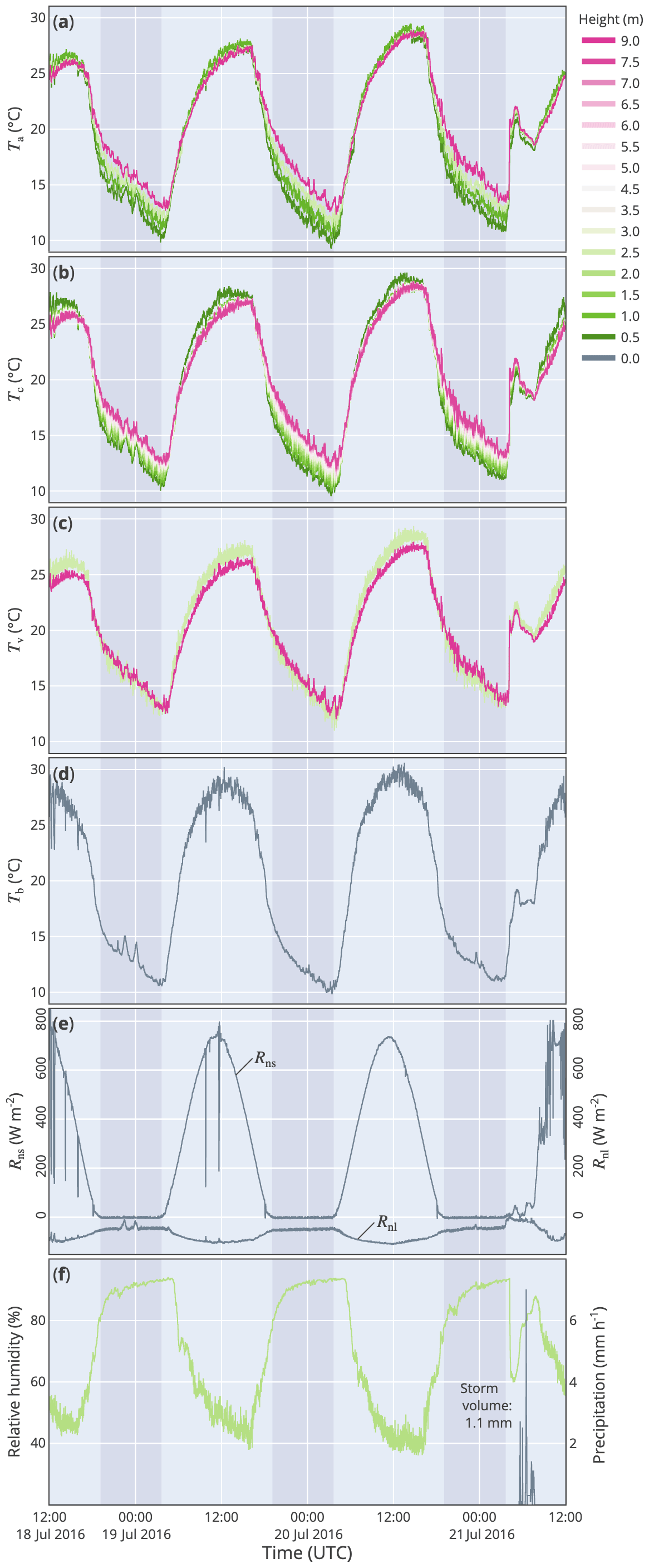
Figure 3The 1 min mean of (a) air temperature, (b) air temperature from fibre-optic cable, (c) air temperature from the speed of sound, (d) surface brightness temperature from radiance (e) net short-wave radiation, Rns, and net long-wave radiation, Rnl, terms, and (f) relative humidity and precipitation.
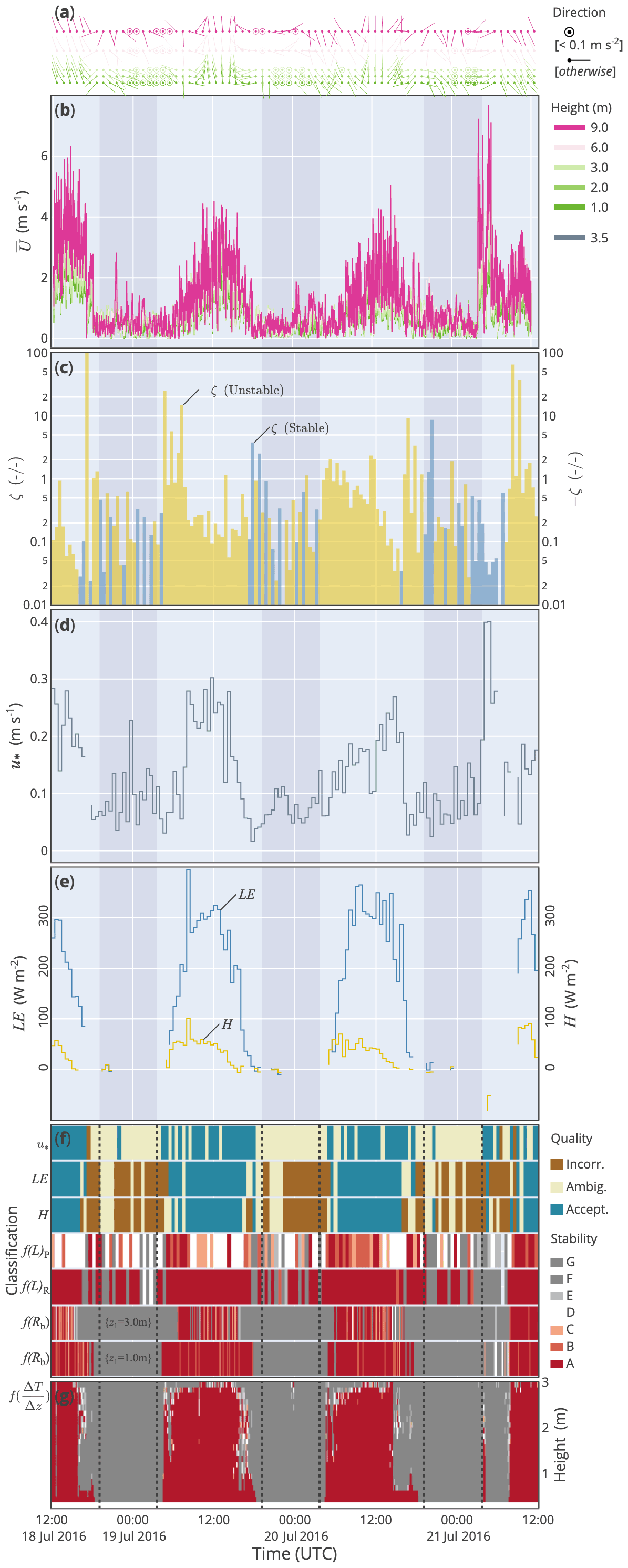
Figure 4The 30 min mean height profile of (a) wind direction, (b) wind speed, and for 3 m height the (c) the stability length parameter, (d) the friction velocity, (e) latent heat (LE) and sensible heat (H) flux, (f) quality and stability classification, and (g) stability against height. See text for details.
3.2 Temperature
The air temperature observations agree between the methods (Fig. 3a–c). Some dissimilarity between Ta and Tc can be seen at the lowest part of the profile (<0.5 m) during the day, where the effects of sensor shading and aspiration on Ta can be expected to be most pronounced (Fig. 3a–b). A stable temperature profile develops at night in excess of 3 K in the lowest 9 m depth (Figs. 3a–c, 5a–b). The unstable daytime temperature gradient is small in comparison, but temperature variance can be significantly larger and increases towards the surface (Fig. 5c–f, g, positive kurtosis). Furthermore, the shape of the variance distribution of those daytime observations indicates a moderate dominance of short-term hot excursions from the mean (Fig. 5g, positive skew). Those are not new findings but again describe the general conditions at the site.
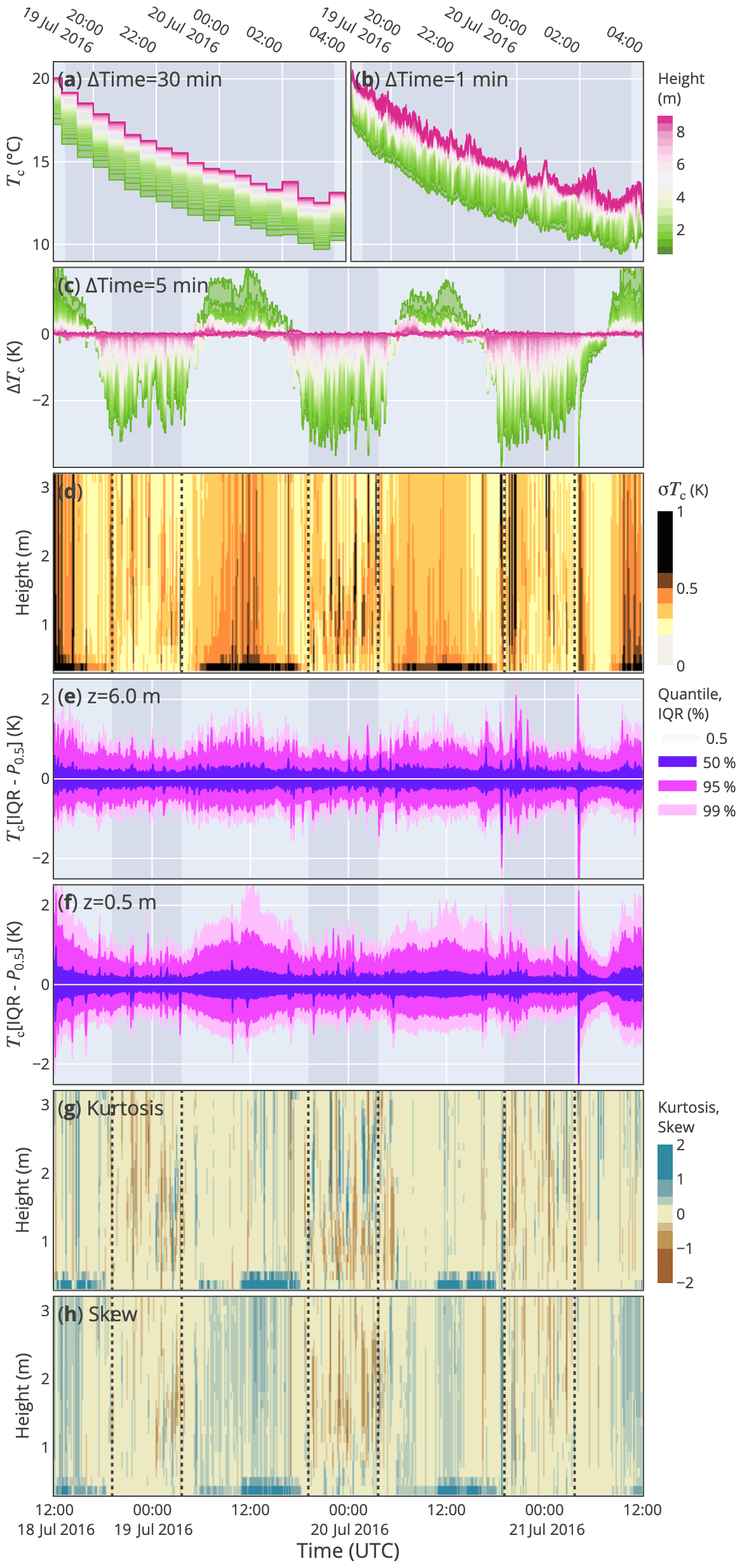
Figure 5Shown against time are (a, b) fibre-optic cable temperature (Tc) for a selected night and 30 and 1 min averaging, respectively, (c) the Tc gradient relative to the top of the profile, (d) the Tc variance against height, (e, f) the interquartile range (IQR) relative to the median (P0.5) for 6.0 and 0.5 m above ground, respectively, (g) the kurtosis and skewness of Tc against height, respectively.
3.3 Temperature timescale decomposition
In addition to aggregating statistics for fixed time intervals, we can decompose the air temperature signal in contributing timescales (Fig. 6). The MRD results confirm a variance maximum at the surface during the day, but at night the dominant contribution was found between 0.5 and 2.5 m depth (Fig. 6b; details about MRD are in Appendix B). Not surprisingly, highest daytime variance was found after the rainstorm on 21 July 2016 under wet surface conditions (Figs. 3f, 5, 6b). During the day, scales of less than 3 min contributed most to total variance, whereas periods of 5 min or more were prominent at night (Fig. 6c). For each of the decomposition levels, we can determine a height of maximum contribution to variance. During the day, a peak contribution was observed at the bottom of the profile, also corresponding to higher decomposition levels (M>7, lower frequency signal). During the day, the sunlit surface acts as a slow-response buffer in the transfer of energy to the air in closest contact. The height of the maximum variance for smaller decomposition scales (M<6, higher frequency contribution) was shown to transition from below 0.5 m before noon, to the top of the profile. During the night, the height of the variance maximum for the large and small decomposition levels could be found to coincide, as shown between 1 and 2 m depth on the night of 19 to 20 July 2016 (Fig. 6d). The simultaneous occurrence of multiple scales at the same location (height) and time suggests an interaction, perhaps cascading of energy from one scale to another.
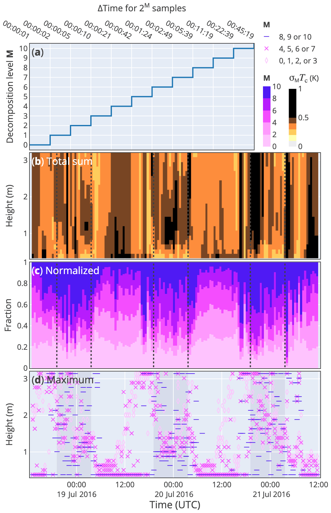
Figure 6Shown for the MRD of Tc are (a) the decomposition levels (M), and against time and height (b) the total sum of variance, σMTc, (c) the relative contribution of each level and (d) the height of maximum mean variance for three groups of M.
The decomposed variance scales for the surface brightness temperature differ in distinct aspects but generally follow a similar pattern (Fig. 7). Similar to Tc, there is a increase in contribution of lower decomposition levels (M<7, higher frequency signal) during the day (Fig. 7b). However, the total variance at the surface is very low during the night (Fig. 7c). This confirms the results for Tc and suggests that the stable stratification at night allows the air (a layer) closest to the vegetation to decouple from the atmosphere aloft. Interestingly, spatial patterns do emerge from the Tb variance that correlate to location, also at night when total variance is very low. This is discussed in more detail in Sect. 3.5.
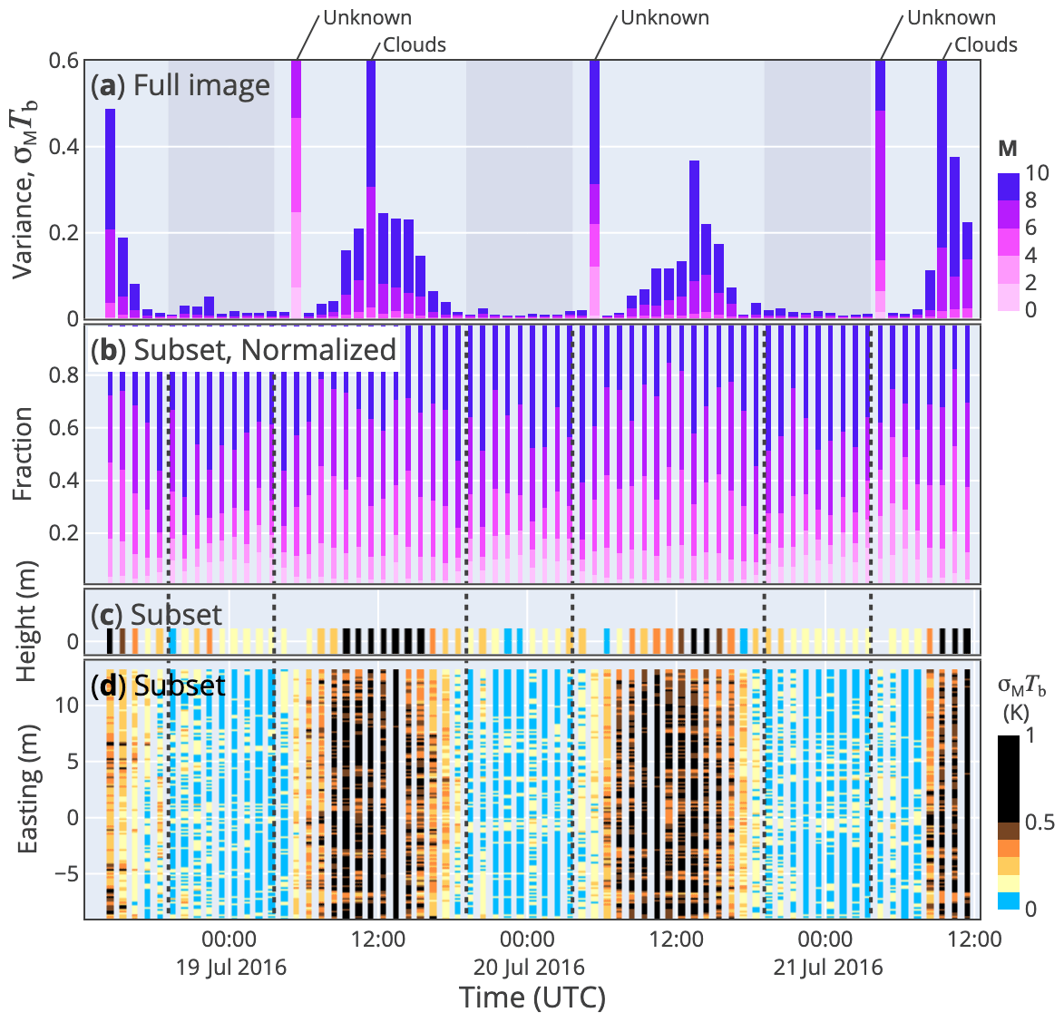
Figure 7Shown against time for the MRD of Tb are (a) the sum of variance for the full thermal image, (b) the relative contribution of each decomposition level, (c) the total sum of variance, σMTb, and (d) the total sum of variance per grid cell in a subset image area. The subset includes grid cells depicting vegetation within 1 m of a fibre-optic profile, for which the cell location is expressed relative to the centre of the domain. See text for details.
Please note that the MRD results helped identify noise peaks affecting the whole thermal image in the early morning on most days. This noise signal is likely caused by direct sunlight at very low zenith angles (Fig. 7a). Furthermore, the Tb signal shows limited information in the lowest decomposition scales (M<2, high frequency), which is assumed to be a design feature of the camera and likely governed by noise-reduction algorithms that result in a low temporal sensitivity. The Tc results contain more high-frequency signal than the Tb, as is evident from the lowest decomposition levels and typical for lidar data such as DTS.
3.4 Temperature event classification
The MRD and other decomposition methods, such as wavelet, help decompose variance in time, but do not necessarily discern the shape of the variance events. In fact, the outcomes of MRD differ substantially between a signal with sine wave or ramp shape, which both commonly occur in air temperature time series. For the same event duration, MRD can classify a wave and a ramp shape one decomposition level apart. It is therefore helpful to investigate the shape of variance events in more detail. An indicator for event shapes that likely show a more sawtooth or ramp-like pattern is positive skewness. The difference between the first half and second half of the event provides addition detail. Such statistical features can be used to identify events, and this is the basis of methods like TED (Kang et al., 2013, 2015, see Appendix B). The original TED classification is based on differences between variance events in Euclidean space, i.e. k-means clustering on principle components analysis of event statistics. Different event types may occur throughout the day and throughout the vertical profile (Fig. 8). The classification of some clusters appeared to coincide with the timing and height of dominant variance scales identified and localised by MRD (Fig. 6d). This is seen most clearly at night.

Figure 8Shown for each TED-determined cluster are the number of events per 30 min time interval and height. The clusters are ranked according to frequency, with the least frequent in the bottom panel.
The accuracy of event classification statistics dependents on the signal and the ability to separate the noise it includes. We do not investigate here how such statistical event features translate between different sensor types with different noise profiles. Further analysis of lagged spatial correlations would be beneficial for the identification of patterns and the evolution of structures, which the applied algorithms currently do not address.
3.5 Spatial temperature patterns
Based on the scale decomposition and cluster results, we focus on a nighttime and daytime period more closely, starting 03:00 UTC 20 July 2016 and 10:00 UTC 21 July 2016, respectively. An example of night and daytime observations can be viewed in an animation (see video supplement). During the daytime animated period, the mean wind is mostly aligned with the DTS measurement setup, i.e. either perpendicular or parallel to the walls of the box-shaped array, with mean flow from a SSE direction. Both the daytime and nighttime cases show intermittent structures. However, animations reveal scale interactions that are not easily identified in the decomposition or classification statistics.
The surface was not homogeneous in terms of TIR signature. Some signals in the TIR image time series were revealed when and where the background (the surface) and foreground (air that had interacted with a surface upstream) show a different heat signature. Therefore, motion was revealed from hot air advecting away from relatively hot areas in the plant canopy, against a background of cooler surfaces. First, hot plumes or thermal streets advect laterally through the observation volume during the day and appear correlated with streamwise-oriented hot and cold streaks on the surface. The plumes maintain a moderately constant spanwise position (Fig. 9). Motion of the heat structures is not necessarily aligned with the mean wind as recorded by the EC profiles. Please note that this is in part an issue of apparent (covariant) alignment of the vertical planes with the flow (Zeeman et al., 2015). Surface heat emits from hot areas in the vegetation, which are mostly sunlit leaves at the top of the canopy. Remnants of tractor tracks are visible parallel to the DTS setup and field track in a WSW to ENE direction (Fig. A5; on close inspection also in Fig. 2). The vegetation canopy was higher where tractor tires did not disturb the soil and vegetation during the previous harvest. The streaks of hot and cold air appear to move independently of the orientation of those tracks, although a hot Tb signal shows up more clearly against the cool background of low vegetation in the tractor tracks, making its visual appearance dependent on the approach use here in which all variance scales are included. It is assumable that patterns in thermal brightness signal relate to heat and moisture released by evapotranspiration, where variability in moisture contributes to a spatial differentiation in emissivity. Those emissivity values are unknown; hence, the Tb signal is not necessarily an accurate measure of Ts. Nevertheless, we can clearly identify structures from motion in the Tb signal during the day. Analyses of decomposed Tc signal are needed to accurately distinguish the heterogeneity in the transmission of heat, related to canopy structure. Second, occasionally, gusts cause divergent motion at the surface, revealed in Tb as cold patches that are reminiscent of gust landing on flat water, forming so-called capillary waves (see, e.g. Dorman and Mollo-Christensen, 1973). Third, shear-induced wave and wave-breaking patterns were shown at multiple scales in the nighttime case, but no clear signal was found in Tb at the surface (Fig. 10). The location of the shear (and wave) interfaces coincided with the MRD- and TED-determined heights for variance maxima discussed above. Most nighttime events correlated with wind direction shifts in the profile. Wind shear events were shown to cause cascades of ripples, which occasionally are only visible in one section of Tc but not elsewhere, suggesting the disturbances could be local.
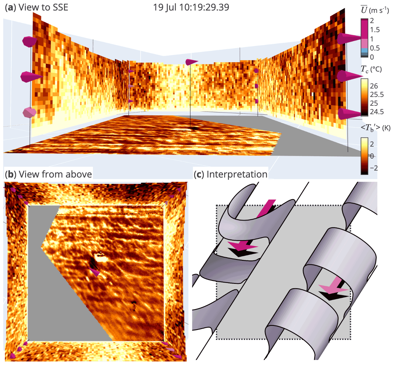
Figure 9Daytime example of structures and motion in air and surface temperature represented by fibre-optic cable temperature (Tc) and surface brightness temperature (Tb) variance, respectively. Shown are (a) a viewpoint from NNW, (b) a perspective from above and (c) a conceptual interpretation. Observations of wind are shown as cones pointing in the direction of the mean wind ().
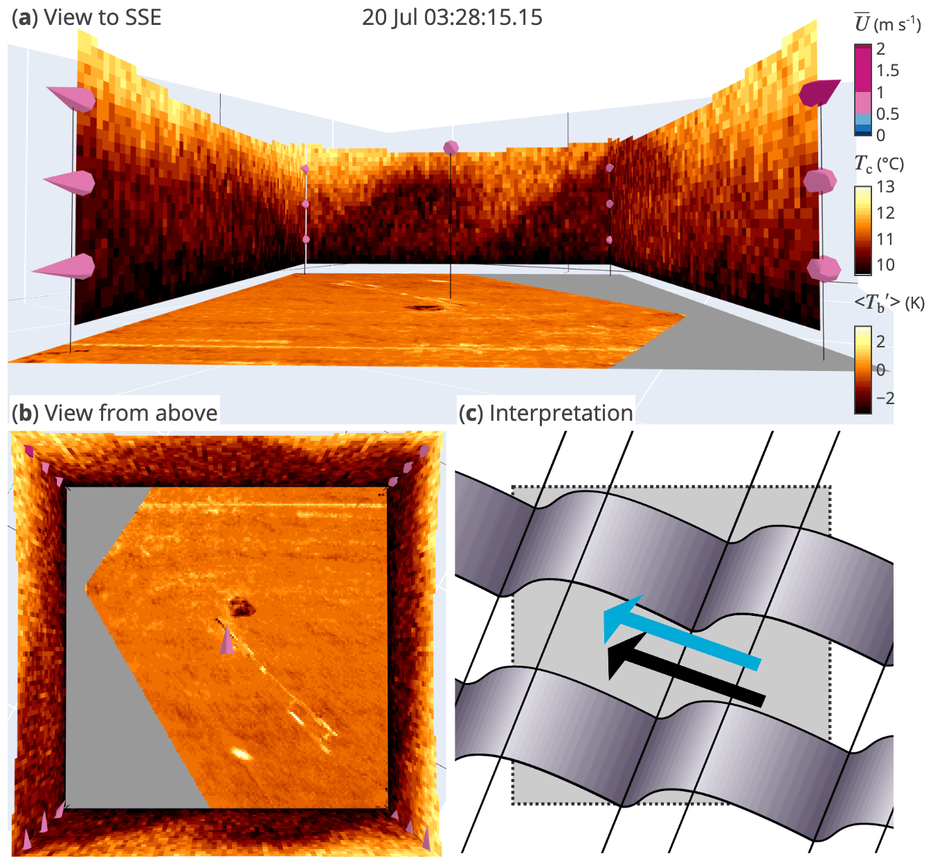
Figure 10Nighttime example of structures and motion in air and surface temperature represented by fibre-optic cable temperature (Tc) and surface brightness temperature (Tb) variance, respectively. Shown are (a) a viewpoint from NNW, (b) a perspective from above and (c) a conceptual interpretation. Observations of wind are shown as cones pointing in the direction of the mean wind ().
The computed turbulent kinetic energy (TKE, ) supports this observation (Fig. 11). Although TKE is an order of magnitude lower during the night than during the day, peaks that did occur at 3 m were not necessarily registered at all corners of the observation domain, or at others heights in the profile. A peak at 3.0 m at 03:28 UTC on 20 July 2016 exemplifies this (Figs. 11b and 10). The decomposed variance and identified clusters for this event provided further evidence that the wave interaction did not perturb the air closest to the surface (Fig. 12). Classified TED events were detected at the same height as the variance maximum from the MRD decomposition, but an exact match to the timing of dominant variance peaks and structures did not occur. Possible explanations were the minimum event window size of approximately 120 s and the effect of high-frequency noise in the Tc time series. Please note that these particular nighttime events are characterised by abrupt negative temperature anomalies. A sudden jump in TKE shortly after sunrise on 21 July 2016 is correlated with the passing of a brief rainstorm (Figs. 11c, 3f, 4b).
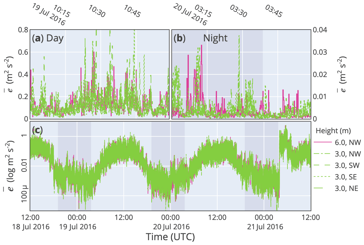
Figure 11The turbulent kinetic energy (TKE; ) was computed for corner locations at 3.0 or 6.0 m above ground and shown for (a) an example daytime hour, (b) and an example nighttime-to-dusk hour and (c) the study period. Nighttime is highlighted with dark areas.
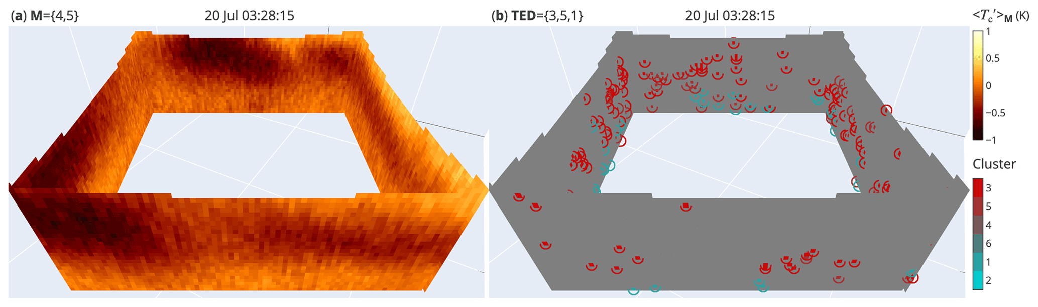
Figure 12Shown for a nighttime instance are (a) the variance for selected MRD levels (M) of Tc and (b) the dominant clusters corresponding to detected events within a 45 s window. See text for details.
The Tc and Tb methods resolve an order of magnitude more locations than Tv or Ta data but can only reveal structures that exhibit substantial temperature differences and spatial (auto)correlation. Combining the observations of horizontal and vertical planes allows combined investigation of spanwise and streamwise correlations. A decomposition along multiple dimensions (e.g. two-dimensional space), a classification of two-dimensional shape features and the quantification of time-sequential motion are outside the scope of this study.
3.6 Experimental design
There are limitations in the described approach using DTS and TIR data which would require further thought on experimental design. First, the support structures of the fibre-optics and other sensors were placed as far away as practicable with a suspension cable system (Appendix A3.1), but this did not prevent shadows on the surface and profiles at lower zenith angles. The shadow effects are systematic and can be overcome by careful selection of data points. Vertical shadows are less of a concern, as these affect only a small number of vertical profiles at a time, and nighttime data are less affected. Second, a circle-shaped geometry for the fibre-optic cable setup would make up- and downwind pairs equidistant, potentially simplifying analysis by making the lateral gradients independent of wind direction. Third, in retrospect after analysis, placement of three-dimensional sonic anemometers at lower heights in the profile would have been advantageous. It would have been informative to compare vertical wind speed, TKE and stability information to height levels of interest below 3 m. Fourth, parallax issues caused by objects in view of the thermal camera can only be overcome by using multiple cameras from different viewpoints. An uncluttered, regular grid matrix is helpful for time-sequential analysis of motion, for instance, using algorithms developed in computer vision research. Fifth, continuous thermal imaging data would be needed. The hourly interruption of the recording of Tb in this experiment was caused by a meanwhile-resolved software issue. Sixth, the addition of a reference surface temperature measurement within view of the TIR camera will be useful for the assessment of noise in the image time sequence. Seventh, the use of a thinner fibre-optic cable design with a lower thermal inertia could improve the Tc response, although the sensitivity of DTS technique may become a limitation at high recording frequencies (see Appendix A3; 0.2 K white noise at 0.5 Hz). Eighth, the TED skill may be improved with the information from the scale decomposition, e.g. by applying the method on a variance subset from which high- and low-frequency contributions are excluded. Ninth, the use of supervised machine learning techniques benefits from the availability of statistical features with a physical meaning. The use of additional event metrics, particularly those supported by past research on RSL processes, should be explored. Even simplified stability indicators could turn out useful for data exploration, in favour of the moderately high computational costs of signal decomposition (e.g. MRD and TED) applied to high-resolution sensor networks.
Despite accuracy drawbacks, current DTS and TIR applications promise frequent (0.2 Hz or better), moderately precise (0.2 K or better) and highly localised (0.25 m or better) observations of thermal signal in a spatial domain suitable for micrometeorological applications near the surface (in 2.5 dimensions or better). The fingerprints of motion and turbulence structure could be identified in horizontal and vertical planes. Horizontal and vertical cross-sections allow a tomographic investigation of spanwise and streamwise organised motion, in a novel combination with time-sequential thermography. However, small-scale turbulence is difficult to resolve due to the heterogeneous thermal properties of the vegetation surface and sensor precision at short signal integration times. The heterogeneity in thermal activity of the vegetation points at ecophysiological traits that may be contributing factors in the formation and distribution of coherent structures near the surface, which needs to be investigated further. The ability to trace coherent motion in space and time may proof useful for the development of conditional sampling methods that complement the eddy-covariance technique. The comparability of TED results between time series could be improved with a (hybrid-)hierarchical clustering modification, but the modifications only partly resolved limitations of repeatability of the cluster analysis. The identification and classification of events in turbulence time series will benefit from the development of physics-aware machine learning techniques that quantify combinations of scale and shape features, instead of treating those as separate properties. In addition, a supervised approach for event detection using machine learning techniques may lead to new avenues for investigation of turbulence interactions near the surface from increasingly high-resolution observations of atmospheric properties.
A1 Time synchronisation
Sensor data from each EC profile were recorded by a datalogger system with accurate time keeping, comprising a low-power computer (model Beaglebone Black, BeagleBoard.org Foundation, Oakland Twp, MI, USA), four digital communication ports (RS232), a temperature-compensated hardware clock (model ChronoDot, DS3231; Maxim Integrated Products Inc., San Jose, CA, USA) operated by a modified operating system with accurate time synchronisation (Debian Linux; Chrony software module). In addition, an asynchronous network framework was used to record up to four EC sensors simultaneously with low latency (Python 2.7; Twisted software module). Similar systems were used as time reference device in the local computer networks of the DTS and TIR, recording time offset continuously. The time offset between the data logging systems was determined before, during and after the campaign and showed no measurable drift. A GPS unit was used as a backup reference to world time, as access to internet real-time services could not be guaranteed at all times. Please note that time is reported in UTC, but local time was CEST (UTC+2; CET summer time).
A2 Georeferencing
The EC and TIR sensors were referenced by measurement tape compared to the central EC location (ICOS station). The same was done for the rings used in the support structure for the DTS fibre-optic cable.
A2.1 Wind direction
The orientation of each sonic anemometer was determined using a magnetic compass. However, this appeared imprecise, and relative offsets () were determined from a period of data with strong wind from a persistent N direction, along the valley axis. The wind vectors in all EC time series were corrected accordingly.
A2.2 Fibre-optic cable
The DTS fibre cable was suspended using white rings with grooves in which the fibre-optic cable was held in place by gravity and light tension (Fig. A1). All coils and turns made with the fibre-optic cable throughout the setup, including the temperature calibration, were made to match the diameter of the grooves of these rings (cut from polypropylene drainage pipe; Ø 0.25 m). The rings were kept in place and aligned with a support cable through the centre of the ring. The locations of the straight vertical sections were initially identified in the DTS signal with ice packs at known locations. However, the fibre-optic cable developed in the initial days of deployment (June 2016, prior to the experiment), as the material of the outer jacket stretched under heat and tension until it matched the almost non-elastic Kevlar buffer. Slack in the fibre-optic cables was removed by adding tension to the steel suspension cables using pulleys and by coiling excess cable on the bottom rings. As the position of some sections of cable could still change, e.g. accidentally or by re-adjustment, the locations of the straight vertical sections were re-confirmed by detection of peaks in signal attenuation (Stokes signal) that correlate to the bend sections of fibre on the rings, as well as temperature differences at noon (bottom rings are warm, compared to top) and after sundown (bottom rings are cold, compared to top). The latter also helped confirm the direction and height of each vertical profile (Figs. A2, A3). The algorithm to detect ring-coiled sections of cable used a combination of (wavelet) filters on the DTS signals and their derivatives, including minima, maxima and zero-crossing points in and , where xi is the DTS range-gate interval distance along the fibre. The optical fibre is packaged loosely inside the cable with up to 10 % “overstuff”; hence, measurements along the cable exterior are only an approximation of location of DTS range gates. A 0.15 m section along the fibre translated to a fibre-optic cable section of approximately 0.125 m.
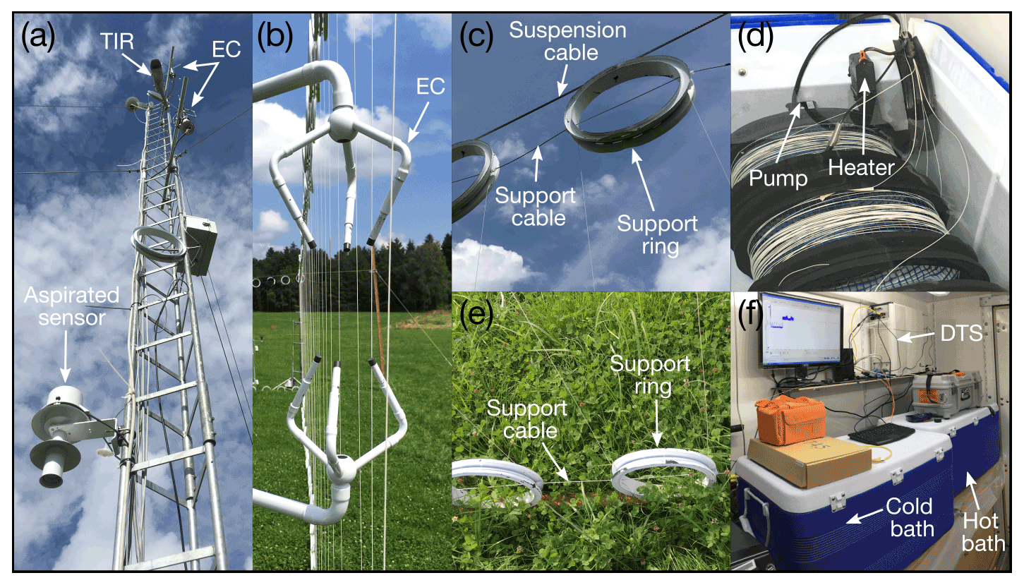
Figure A1Details of the field setup showing (a) a close-up of the 9 m mast, (b) a view along a vertical plane of DTS profiles, (c, e) details of the DTS support structure, (d) a view inside a calibration bath and (f) the DTS instrumentation.
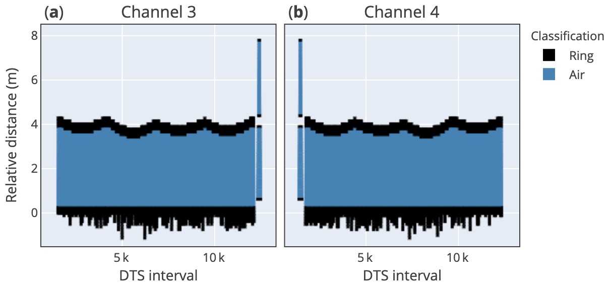
Figure A2The distance relative to the lower support rings were determined for DTS intervals in (a, b) opposite sensing directions. Intervals in contact with the rings were excluded from the analysis, leaving 8286 usable locations.
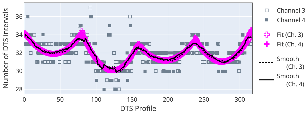
Figure A3The alignment of DTS profiles was validated using a fit (hyperbole cosine) and smoothing (Savitzky–Golay) function.
A2.3 Image projection
To map image pixels to real-world locations, the lens optical distortion was determined, as well as the location, the height, and the roll, pitch and yaw rotation of the sensor (Fig. A4). The spatial resolution at the surface varied with distance away from the mast due to camera perspective and parallax. To facilitate computation, the image time series were resampled to a regular 0.125 m grid, aligned with the spatial resolution and orientation of the DTS setup (Figs. A4, A5), excluding pixels far outside the 20×20 m domain or depicting objects. For the translation from a perspective view to an orthogonal map, the surface was assumed to be flat.

Figure A4The projection of thermal images to real-world coordinates required (a) correction for lens optical distortion and (b) project after camera rotation. The numbers refer to pixel count relative to the image top-left corner.
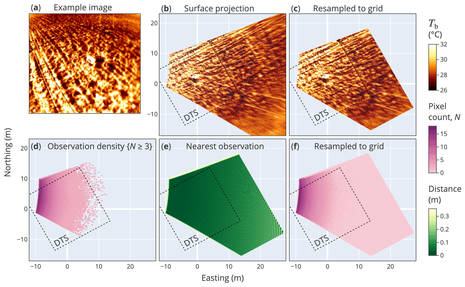
Figure A5The (a, b) thermal image data were (c, f) spatially resampled in a regular grid of 0.25×0.25 m, matching the orientation of the fibre-optic array (DTS). At least (d) three observations should fall within a grid cell, or else (e) the nearest value within a 0.35 m radius was used for computation.
A3 Temperature reference
A3.1 DTS cable temperature (Tc)
The DTS observations were calibrated using reference temperature measurements. Reference temperature sensors (two PT-1000 probes) are an integral part of the DTS instrument and recorded automatically. The sensors were placed inside two insulated water baths in close proximity to sections of fibre-optic cable. One bath was heated using an aquarium heater (32 ∘C; model Fluval E-100, Hagen GmbH, Holm, Germany), the other bath was chilled using a laboratory flow-through cooler (4 ∘C; model Titan 500, AB Aqua Medic GmbH, Bissendorf, Germany), and both baths were continuously mixed using aquarium pumps (10 L min−1 flow rate, directed horizontally at half depth; model PondoCompact 600, PonTec, Hörstel, Germany). At both ends of the fibre-optic cable and in both calibration baths, at least 20 m of cable was placed loosely on a submerged spool made of mesh material, in order to keep the cable away from the walls of the bath and achieve temperature equilibrium with the water. For each measurement, the span and offset values determined for both ends of the cable were linearly interpolated and applied to all intervals in between the calibration sections (see, e.g. Hausner et al., 2011; Zeeman et al., 2015). Between 0.1 and 0.2 K of variance can be attributed to white noise, as shown from an Allan deviation plot on data before calibration (Fig. A6; see, e.g. Werle, 2010).
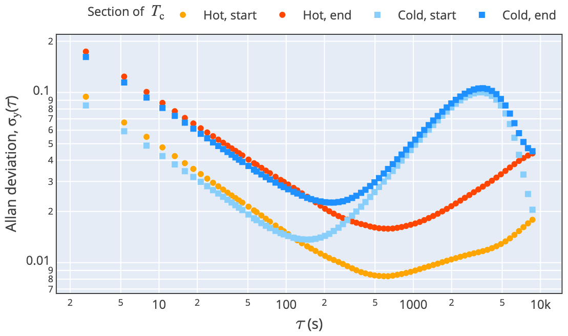
Figure A6Allan deviation for four DTS range gates in different sections of the fibre-optic cable, in cold and hot baths and at the start and end of the cable, respectively. The −1 slope towards high frequency (τ<100 s) indicates white noise. Calculations were made before calibration on 24 h of Tc data.
A3.2 TIR brightness temperature (Tb)
The imaging data were converted to a time series of brightness temperature assuming an emissivity of 0.96. However, a high-frequency noise was found in the time series that affected the whole image. The signal was assumed to be an artefact of small variations in the exposure time of the detector and sensitivity to the interruptions by the automatic self-calibration mechanism. The signal could effectively be removed by subtracting the mean temperature of the whole image (or a selected area) from the value of each pixel. Although this effectively applies a high-pass filter in the time domain, the image data are improved in a meaningful way for the applicability of time-sequential thermography.
A3.3 EC temperature from speed of sound (Ts)
A measure of temperature can be derived from the speed of sound and is commonly provided as computed records directly from the three-axis ultrasonic anemometers (Table 1). The EC sensors therefore require factory calibration for temperature. In addition, a cross-validation of Ts was performed based on a period of operation prior to this experiment during which all sonic anemometers were installed at equal height (Mauder and Zeeman, 2018).
A3.4 Aspirated air temperature (Ta)
Air temperature measurements were made with resistance temperature devices in fan-aspirated enclosures at four heights along the mast (RTD PT1000; models 41347 and 43502, R.M. Young Company, Traverse City, MI, USA; see Table 1) and recorded at 0.5 Hz (model CR5000, Campbell Scientific Inc, Logan, UT, USA). The temperature sensors were calibrated for span and offset prior to the campaign using a well-mixed water bath (see Appendix A3.1), while increasing the temperature along an approximate ambient range (18–27 ∘C; PT100 based digital thermometer, model GMH 3710, Greisinger Electronics GmbH, Regenstauf, Germany; Wolz, 2016).
A3.5 Cross-comparison
A comparison was made between temperature measurements by the different systems, using sensors that were closely located in space (Table 1). For the cross-comparison, sensors were selected nearest to the Ta observations at 3 m height and during a period with an approximately equal number of daytime and nighttime hours (12:00 UTC 19 July 2016 to 04:00 UTC 20 July 2016). The results show that both Tc and Ts are linearly correlated with Ta but did not exactly match the aspirated temperature in absolute value and high frequency variance (Fig. A7). The Ta sensors exhibit a slower thermal constant due to the size of the metal sensor rod, leading to a dampened high-frequency response compared to Ts and TcḞurthermore, Ts was cross-calibrated among the EC sensors prior to this experiment, but not calibrated against a temperature reference scale (Mauder and Zeeman, 2018). This shows a need to include the calibration of Ts in future experiments. However, differences between aspirated and non-aspirated sensing methods are inevitable and explain part of the deviation between sensing systems seen here. A comparison between Tc and Ts showed linearity between the signals, which appeared to improve during the night in the absence of direct solar radiation (Fig. A7). However, the computed coherence between Tc and Ts deteriorated at high frequency (>0.1 Hz; Fig. A7d). This can in part be explained by noise in one or both of the systems, as well as small differences between the locality and path length of the sensors being compared.
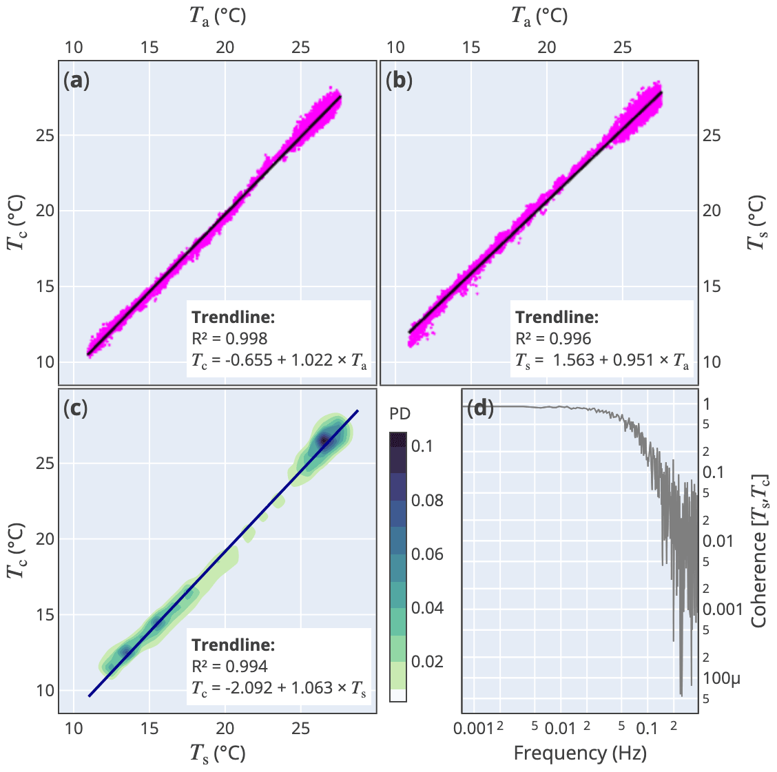
Figure A7Shown are the correlation between (a) Ta and Ts, (b) Ta and Tc, and (c) Ts and Tc as colour contours representing probability density (PD), as well as (d) the coherence between Ts and Tc against frequency.
A4 System integration
Some additional measures were needed to integrate all systems. In order to avoid AC power hazards, to limit electrical cross-interference and to accommodate voltage drops on long cables, all outdoor devices were connected to a central 24 V DC power supply and grounding to earth, with subsequent local downregulation to 5 or 12 V DC. Similarly, network connections were made using fibre-optic links instead of metal wire cables. The DTS system, including a temperature calibration setup, was operated inside a temperate-regulated housing. To accommodate data storage requirements for continuous operation, all data were automatically transferred on an hourly (DTS, TIR) or daily (EC) basis. Python was used for data acquisition, analysis and figures (Python 3.7; Hoyer and Hamman, 2017; Virtanen et al., 2020; Anaconda, 2020; Plotly Technologies Inc., 2020), with additional analysis produced by R (R Core Team, 2018; Sarkar, 2008; Wickham et al., 2020).
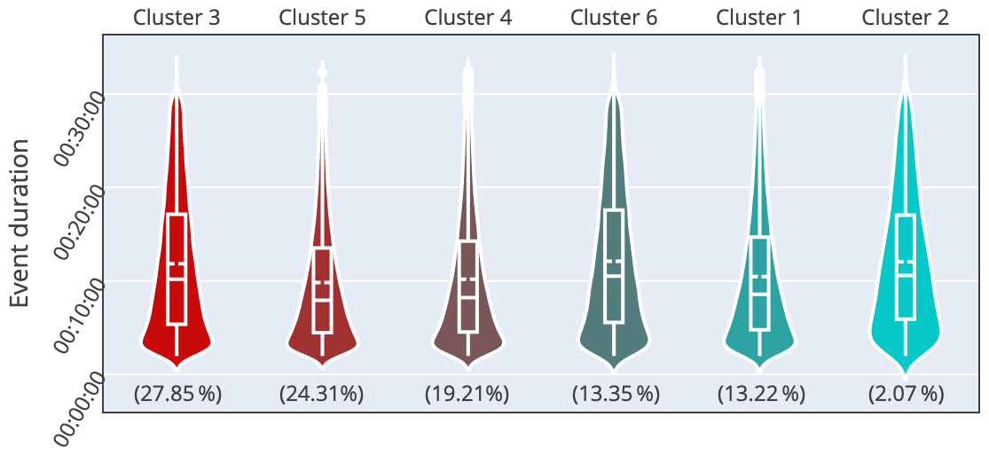
Figure A8The TED method samples events in temperature time series and applies a k-means clustering on event statistics. Clusters are ranked by fraction of total events, shown as percentage below the violin-box-plot distribution of the event duration.
The comparison of computed variables included
where [z1>z2];
where [z1>z2];
where is the total horizontal wind velocity, is the turbulent kinetic energy (TKE), u* is the friction velocity, ΔT is the vertical temperature gradient, RB is the bulk Richardson number, with z the height above ground and g the acceleration due to gravity, L is the Obukhov length with κ the von Karman constant, and ζ is a dimensionless scaling parameter (Stull, 1988). The overbars denote averaging in time. Double rotation refers to a method of alignment of the coordinate system into the mean wind (Kaimal and Finnigan, 1994). Stability classes were taken from literature and repeated for completion in Table B1.
Pasquill (1961)Gifford (1976)Pasquill and Smith (1971)Gryning et al. (2007)Woodward (1998)Table B1Stability categories and Pasquill–Gifford classes based on literature, as a function of bulk Richardson number (Rb), Obukhov length (L) and the temperature gradient with height. “NA” means “not available”.

Data from this study are available with open access (https://doi.org/10.5281/zenodo.4267888, Zeeman, 2020a; https://doi.org/10.5281/zenodo.4267811 Zeeman, 2020b; and https://doi.org/10.5281/zenodo.4061242, Zeeman, 2021). Software code are available as notebooks for Python and R (https://gitlab.imk-ifu.kit.edu/scalex/, Zeeman, 2020d) or from the author.
The video supplement contains an animation of high-resolution data for a nighttime and daytime hour (https://doi.org/10.5446/50229, Zeeman, 2020c).
The author declares that there is no conflict of interest.
Publisher’s note: Copernicus Publications remains neutral with regard to jurisdictional claims in published maps and institutional affiliations.
Carsten Malchow (KIT) supported the development of systems to suspend fibre-optic cables and to record data from a sensor network, and Janina Klatt (KIT) prepared the ICOS station. Kevin Wolz (student at KIT) assisted in many aspects of the deployment. Peter Brugger, Benjamin Wolf, Rainer Gasche, Nadine Ruehr, Carsten Jahn, Matthias Mauder, Robert Neuner, Joseph Burger, Frank Neidl, Christoph Soergel (all at KIT), Claire Brenner (at BOKU) and Peng Zhao (at U Innsbruck) offered assistance in the field. Martin Schoerner (at U Augsburg) shared aerial video. Tirtha Banerjee, Danijel Belusic, Claire Brenner, Marc Calaf, Rainer Hilland, Marwan Katurji, Benjamin Schumacher and Nikki Vercauteren provided helpful discussion.
This research has been supported by the German Research Foundation (DFG; grant no. ZE1006-2/1) and the Atmosphere and Climate (ATMO) programme of the Helmholtz Association of German Research Centres.
The article processing charges for this open-access publication were covered by the Karlsruhe Institute of Technology (KIT).
This paper was edited by Christian Brümmer and reviewed by Nikolas Angelou and two anonymous referees.
Abram, C., Fond, B., Heyes, A. L., and Beyrau, F.: High-speed planar thermometry and velocimetry using thermographic phosphor particles, Appl. Phys. B, 111, 155–160, https://doi.org/10.1007/s00340-013-5411-8, 2013. a
Anaconda: Anaconda Software Distribution, Version 4–4.8.3, available at: https://anaconda.com (last access: 14 April 2021), 2020. a
Antonia, R. A., Chambers, A. J., Friehe, C. A., and Atta, C. W. V.: Temperature Ramps in the Atmospheric Surface Layer, J. Atmos. Sci., 36, 99–108, https://doi.org/10.1175/1520-0469(1979)036<0099:tritas>2.0.co;2, 1979. a
Aubinet, M., Vesala, T., and Papale, D. (Eds.): Eddy Covariance: A Practical Guide to Measurement and Data Analysis, Springer, https://doi.org/10.1007/978-94-007-2351-1, 2012. a
Bou-Zeid, E., Anderson, W., Katul, G. G., and Mahrt, L.: The Persistent Challenge of Surface Heterogeneity in Boundary-Layer Meteorology: A Review, Bound.-Lay. Meteorol., 177, 227–245, https://doi.org/10.1007/s10546-020-00551-8, 2020. a
Brenner, C., Zeeman, M., Bernhardt, M., and Schulz, K.: Estimation of evapotranspiration of temperate grassland based on high-resolution thermal and visible range imagery from unmanned aerial systems, Int. J. Remote Sens., 39, 5141–5174, https://doi.org/10.1080/01431161.2018.1471550, 2018. a
Brosy, C., Krampf, K., Zeeman, M., Wolf, B., Junkermann, W., Schäfer, K., Emeis, S., and Kunstmann, H.: Simultaneous multicopter-based air sampling and sensing of meteorological variables, Atmos. Meas. Tech., 10, 2773–2784, https://doi.org/10.5194/amt-10-2773-2017, 2017. a
Brutsaert, W.: Land-surface water vapor and sensible heat flux: Spatial variability, homogeneity, and measurement scales, Water Resour. Res., 34, 2433–2442, https://doi.org/10.1029/98WR01340, 1998. a
Burns, P. and Chemel, C.: Evolution of Cold-Air-Pooling Processes in Complex Terrain, Bound.-Lay. Meteorol., 150, 423–447, https://doi.org/10.1007/s10546-013-9885-z, 2014. a
Christen, A., Meier, F., and Scherer, D.: High-frequency fluctuations of surface temperatures in an urban environment, Theor. Appl. Climatol., 108, 301–324, https://doi.org/10.1007/s00704-011-0521-x, 2011. a
Clement, R. J. and Moncrieff, J. B.: A Functional Approach to Vertical Turbulent Transport of Scalars in the Atmospheric Surface Layer, Bound.-Lay. Meteorol., 173, 373–408, https://doi.org/10.1007/s10546-019-00474-z, 2019. a
Dakin, J., Pratt, D., Bibby, G., and Ross, J.: Distributed optical fibre Raman temperature sensor using a semiconductor light source and detector, Electron. Lett., 21, 569–570, https://doi.org/10.1049/el:19850402, 1985. a
de Jong, S. A. P., Slingerland, J. D., and van de Giesen, N. C.: Fiber optic distributed temperature sensing for the determination of air temperature, Atmos. Meas. Tech., 8, 335–339, https://doi.org/10.5194/amt-8-335-2015, 2015. a
Dorman, G. E. and Mollo-Christensen, E.: Observation of the Structure on Moving Gust Patterns Over a Water Surface (“Cat's Paws”), J. Phys. Oceanogr., 3, 120–132, https://doi.org/10.1175/1520-0485(1973)003<0120:ootsom>2.0.co;2, 1973. a
Euser, T., Luxemburg, W. M. J., Everson, C. S., Mengistu, M. G., Clulow, A. D., and Bastiaanssen, W. G. M.: A new method to measure Bowen ratios using high-resolution vertical dry and wet bulb temperature profiles, Hydrol. Earth Syst. Sci., 18, 2021–2032, https://doi.org/10.5194/hess-18-2021-2014, 2014. a
Finnigan, J.: Turbulence in Plant Canopies, Annu. Rev. Fluid Mech., 32, 519–571, https://doi.org/10.1146/annurev.fluid.32.1.519, 2000. a
Finnigan, J. J.: Turbulence In Waving Wheat: I. Mean Statistics And Honami, Bound.-Lay. Meteorol., 16, 181–211, https://doi.org/10.1007/BF02350511, 1979. a
Foken, T.: 50 Years of the Monin–Obukhov Similarity Theory, Bound.-Lay. Meteorol., 119, 431–447, https://doi.org/10.1007/s10546-006-9048-6, 2006. a
Garratt, J. R.: Surface influence upon vertical profiles in the atmospheric near-surface layer, Q. J. Roy. Meteorol. Soc., 106, 803–819, https://doi.org/10.1002/qj.49710645011, 1980. a, b
Gifford, F. A.: Turbulent diffusion-typing schemes: a review, Nucl. Saf., 17, 68–86, 1976. a
Gryning, S.-E., Batchvarova, E., Brümmer, B., Jørgensen, H., and Larsen, S.: On the extension of the wind profile over homogeneous terrain beyond the surface boundary layer, Bound.-Lay. Meteorol., 124, 251–268, https://doi.org/10.1007/s10546-007-9166-9, 2007. a
Hald, C., Zeeman, M., Laux, P., Mauder, M., and Kunstmann, H.: Large-eddy simulations of real world episodes in complex terrain based on ERA-Reanalysis and validated by ground-based remote sensing data, Mon. Weather Rev., 147, 4325–4343, https://doi.org/10.1175/mwr-d-19-0016.1, 2019. a
Hausner, M. B., Suárez, F., Glander, K. E., Giesen, N. v. d., Selker, J. S., and Tyler, S. W.: Calibrating Single-Ended Fiber-Optic Raman Spectra Distributed Temperature Sensing Data, Sensors, 11, 10859–10879, https://doi.org/10.3390/s111110859, 2011. a, b
Higgins, C. W., Katul, G. G., Froidevaux, M., Simeonov, V., and Parlange, M. B.: Are atmospheric surface layer flows ergodic?, Geophys. Res. Lett., 40, 3342–3346, https://doi.org/10.1002/grl.50642, 2013. a
Howell, J. and Mahrt, L.: Multiresolution Flux Decomposition, Bound.-Lay. Meteorol., 83, 117–137, https://doi.org/10.1023/A:1000210427798, 1997. a
Hoyer, S. and Hamman, J.: xarray: N-D labeled arrays and datasets in Python, Journal of Open Research Software, 5, p. 10, https://doi.org/10.5334/jors.148, 2017. a
Ibraim, E., Wolf, B., Harris, E., Gasche, R., Wei, J., Yu, L., Kiese, R., Eggleston, S., Butterbach-Bahl, K., Zeeman, M., Tuzson, B., Emmenegger, L., Six, J., Henne, S., and Mohn, J.: Attribution of N2O sources in a grassland soil with laser spectroscopy based isotopocule analysis, Biogeosciences, 16, 3247–3266, https://doi.org/10.5194/bg-16-3247-2019, 2019. a
Inagaki, A., Kanda, M., Onomura, S., and Kumemura, H.: Thermal Image Velocimetry, Bound.-Lay. Meteorol., 149, 1–18, https://doi.org/10.1007/s10546-013-9832-z, 2013. a
Jones, H. G.: Use of thermography for quantitative studies of spatial and temporal variation of stomatal conductance over leaf surfaces, Plant Cell Environ., 22, 1043–1055, https://doi.org/10.1046/j.1365-3040.1999.00468.x, 1999. a
Kaimal, J. C. and Finnigan, J. J.: Atmospheric boundary layer flows: their structure and measurement. Oxford University Press, New York, USA, 289 pp., 1994. a
Kang, Y., Belušić, D., and Smith-Miles, K.: Detecting and Classifying Events in Noisy Time Series, J. Atmos. Sci., 71, 1090–1104, https://doi.org/10.1175/JAS-D-13-0182.1, 2013. a, b
Kang, Y., Belušić, D., and Smith-Miles, K.: Classes of structures in the stable atmospheric boundary layer, Q. J. Roy. Meteor. Soc., 141, 2057–2069, https://doi.org/10.1002/qj.2501, 2015. a, b, c, d
Katul, G. G., Schieldge, J., Hsieh, C.-I., and Vidakovic, B.: Skin temperature perturbations induced by surface layer turbulence above a grass surface, Water Resour. Res., 34, 1265–1274, https://doi.org/10.1029/98wr00293, 1998. a
Katurji, M. and Zawar-Reza, P.: Forward-Looking Infrared Cameras for Micrometeorological Applications within Vineyards, Sensors, 16, 1518, https://doi.org/10.3390/s16091518, 2016. a
Keller, C. A., Huwald, H., Vollmer, M. K., Wenger, A., Hill, M., Parlange, M. B., and Reimann, S.: Fiber optic distributed temperature sensing for the determination of the nocturnal atmospheric boundary layer height, Atmos. Meas. Tech., 4, 143–149, https://doi.org/10.5194/amt-4-143-2011, 2011. a
Kiese, R., Fersch, B., Baessler, C., Brosy, C., Butterbach-Bahl, K., Chwala, C., Dannenmann, M., Fu, J., Gasche, R., Grote, R., Jahn, C., Klatt, J., Kunstmann, H., Mauder, M., Rödiger, T., Smiatek, G., Soltani, M., Steinbrecher, R., Völksch, I., Werhahn, J., Wolf, B., Zeeman, M., and Schmid, H.: The TERENO Pre-Alpine Observatory: Integrating Meteorological, Hydrological, and Biogeochemical Measurements and Modeling, Vadose Zone J., 17, 180060, https://doi.org/10.2136/vzj2018.03.0060, 2018. a
Kline, S. J., Reynolds, W. C., Schraub, F. A., and Runstadler, P. W.: The structure of turbulent boundary layers, J. Fluid Mech., 30, 741–773, https://doi.org/10.1017/s0022112067001740, 1967. a
Klosterhalfen, A., Graf, A., Brüggemann, N., Drüe, C., Esser, O., González-Dugo, M. P., Heinemann, G., Jacobs, C. M. J., Mauder, M., Moene, A. F., Ney, P., Pütz, T., Rebmann, C., Ramos Rodríguez, M., Scanlon, T. M., Schmidt, M., Steinbrecher, R., Thomas, C. K., Valler, V., Zeeman, M. J., and Vereecken, H.: Source partitioning of H2O and CO2 fluxes based on high-frequency eddy covariance data: a comparison between study sites, Biogeosciences, 16, 1111–1132, https://doi.org/10.5194/bg-16-1111-2019, 2019. a
Knauer, J., Zaehle, S., Medlyn, B. E., Reichstein, M., Williams, C. A., Migliavacca, M., Kauwe, M. G. D., Werner, C., Keitel, C., Kolari, P., Limousin, J.-M., and Linderson, M.-L.: Towards physiologically meaningful water-use efficiency estimates from eddy covariance data, Glob. Change Biol., 24, 694–710, https://doi.org/10.1111/gcb.13893, 2017. a
Kunz, M., Lavric, J. V., Gasche, R., Gerbig, C., Grant, R. H., Koch, F.-T., Schumacher, M., Wolf, B., and Zeeman, M.: Surface flux estimates derived from UAS-based mole fraction measurements by means of a nocturnal boundary layer budget approach, Atmos. Meas. Tech., 13, 1671–1692, https://doi.org/10.5194/amt-13-1671-2020, 2020. a
Kustas, W. and Anderson, M.: Advances in thermal infrared remote sensing for land surface modeling, Agr. Forest Meteorol., 149, 2071–2081, https://doi.org/10.1016/j.agrformet.2009.05.016, 2009. a
Lapo, K., Freundorfer, A., Pfister, L., Schneider, J., Selker, J., and Thomas, C.: Distributed observations of wind direction using microstructures attached to actively heated fiber-optic cables, Atmos. Meas. Tech., 13, 1563–1573, https://doi.org/10.5194/amt-13-1563-2020, 2020. a
Lee, X., Massman, W., and Law, B. (Eds.): Handbook of Micrometeorology, Springer Netherlands, https://doi.org/10.1007/1-4020-2265-4, 2005. a
Li, D., Bou-Zeid, E., and De Bruin, H. A. R.: Monin–Obukhov Similarity Functions for the Structure Parameters of Temperature and Humidity, Bound.-Lay. Meteorol., 145, 45–67, https://doi.org/10.1007/s10546-011-9660-y, 2012. a
Mahrt, L.: The bulk aerodynamic formulation over heterogeneous surfaces, Bound.-Lay. Meteorol., 78, 87–119, https://doi.org/10.1007/bf00122488, 1996. a
Mahrt, L.: Computing turbulent fluxes near the surface: Needed improvements, Agr. Forest Meteorol., 150, 501–509, https://doi.org/10.1016/j.agrformet.2010.01.015, 2010. a
Mauder, M. and Zeeman, M. J.: Field intercomparison of prevailing sonic anemometers, Atmos. Meas. Tech., 11, 249–263, https://doi.org/10.5194/amt-11-249-2018, 2018. a, b, c, d, e
Pasquill, F.: The Estimation of The Dispersion of Windborne Material, Met. Mag., 90, 33–49, 1961. a
Pasquill, F. and Smith, F. B.: The physical and meteorological basis for the estimation of the dispersion of windborne material, in: Proceedings of the Second International Clean Air Congress, edited by: Englund, H. and Beery, W., Academic Press, 1067–1072, https://doi.org/10.1016/B978-0-12-239450-8.50190-8, 1971. a
Patton, E. G., Sullivan, P. P., Shaw, R. H., Finnigan, J. J., and Weil, J. C.: Atmospheric Stability Influences on Coupled Boundary Layer and Canopy Turbulence, J. Atmos. Sci., 73, 1621–1647, https://doi.org/10.1175/jas-d-15-0068.1, 2016. a
Paw U, K. T., Brunet, Y., Collineau, S., Shaw, R. H., Maitani, T., Qiu, J., and Hipps, L.: On coherent structures in turbulence above and within agricultural plant canopies, Agr. Forest Meteorol., 61, 55–68, https://doi.org/10.1016/0168-1923(92)90025-Y, 1992. a
Petrides, A. C., Huff, J., Arik, A., van de Giesen, N., Kennedy, A. M., Thomas, C. K., and Selker, J. S.: Shade estimation over streams using distributed temperature sensing, Water Resour. Res., 47, W07601, https://doi.org/10.1029/2010WR009482, 2011. a
Plotly Technologies Inc.: Collaborative data science, available at: https://plot.ly (last access: 14 April 2021), 2020. a
Poulos, G. S., Blumen, W., Fritts, D. C., Lundquist, J. K., Sun, J., Burns, S. P., Nappo, C., Banta, R., Newsom, R., Cuxart, J., Terradellas, E., Balsley, B., and Jensen, M.: CASES-99: A Comprehensive Investigation of the Stable Nocturnal Boundary Layer, B. Am. Meteorol. Soc., 83, 555–581, https://doi.org/10.1175/1520-0477(2002)083<0555:caciot>2.3.co;2, 2002. a
Raupach, M. R.: Anomalies in Flux-Gradient Relationships Over Forest, Bound.-Lay. Meteorol., 16, 467–486, https://doi.org/10.1007/bf03335385, 1979. a
Raupach, M. R. and Finnigan, J. J.: Scale issues in boundary-layer meteorology: Surface energy balances in heterogeneous terrain, Hydrol. Process., 9, 589–612, https://doi.org/10.1002/hyp.3360090509, 1995. a
R Core Team: R: A Language and Environment for Statistical Computing, R Foundation for Statistical Computing, Vienna, Austria, available at: https://www.R-project.org/, last access: 20 December 2018. a
Sarkar, D.: Lattice: Multivariate Data Visualization with R, Springer, New York, USA, ISBN 978-0-387-75968-5, 2008. a
Sayde, C., Thomas, C. K., Wagner, J., and Selker, J.: High-resolution wind speed measurements using actively heated fiber optics, Geophys. Res. Lett., 42, 10064–10073, https://doi.org/10.1002/2015gl066729, 2015. a
Schilperoort, B., Coenders-Gerrits, M., Luxemburg, W., Jiménez Rodríguez, C., Cisneros Vaca, C., and Savenije, H.: Technical note: Using distributed temperature sensing for Bowen ratio evaporation measurements, Hydrol. Earth Syst. Sci., 22, 819–830, https://doi.org/10.5194/hess-22-819-2018, 2018. a
Schmid, H. P.: Source areas for scalars and scalar fluxes, Bound.-Lay. Meteorol., 67, 293–318, https://doi.org/10.1007/bf00713146, 1994. a
Selker, J. S., Thévenaz, L., Huwald, H., Mallet, A., Luxemburg, W., van de Giesen, N., Stejskal, M., Zeman, J., Westhoff, M., and Parlange, M. B.: Distributed fiber-optic temperature sensing for hydrologic systems, Water Resour. Res., 42, W12202, https://doi.org/10.1029/2006WR005326, 2006. a
Shaw, R. H., Brunet, Y., Finnigan, J. J., and Raupach, M. R.: A wind tunnel study of air flow in waving wheat: Two-point velocity statistics, Bound.-Lay. Meteorol., 76, 349–376, https://doi.org/10.1007/bf00709238, 1995. a
Stull, R. B.: An Introduction to Boundary Layer Meteorology, Kluwer Academic Publishers, Dordrecht, the Netherlands, 1988. a, b
Sun, J., Massman, W., and Grantz, D. A.: Aerodynamic Variables in the Bulk Formulation of Turbulent Fluxes, Bound.-Lay. Meteorol., 91, 109–125, https://doi.org/10.1023/a:1001838832436, 1999. a
Thomas, C., Kennedy, A., Selker, J., Moretti, A., Schroth, M., Smoot, A., Tufillaro, N., and Zeeman, M.: High-resolution fibre-optic temperature sensing: a new tool to study the two-dimensional structure of atmospheric surface-layer flow, Bound.-Lay. Meteorol., 142, 177–192, https://doi.org/10.1007/s10546-011-9672-7, 2012. a, b
Tyler, S. W., Selker, J. S., Hausner, M. B., Hatch, C. E., Torgersen, T., Thodal, C. E., and Schladow, S. G.: Environmental temperature sensing using Raman spectra DTS fiber-optic methods, Water Resour. Res., 45, W00D23, https://doi.org/10.1029/2008WR007052, 2009. a
van Ramshorst, J. G. V., Coenders-Gerrits, M., Schilperoort, B., van de Wiel, B. J. H., Izett, J. G., Selker, J. S., Higgins, C. W., Savenije, H. H. G., and van de Giesen, N. C.: Revisiting wind speed measurements using actively heated fiber optics: a wind tunnel study, Atmos. Meas. Tech., 13, 5423–5439, https://doi.org/10.5194/amt-13-5423-2020, 2020. a
Vickers, D. and Mahrt, L.: The Cospectral Gap and Turbulent Flux Calculations, J. Atmos. Ocean. Tech., 20, 660–672, https://doi.org/10.1175/1520-0426(2003)20<660:TCGATF>2.0.CO;2, 2003. a
Virtanen, P., Gommers, R., Oliphant, T. E., Haberland, M., Reddy, T., Cournapeau, D., Burovski, E., Peterson, P., Weckesser, W., Bright, J., van der Walt, S. J., Brett, M., Wilson, J., Millman, K. J., Mayorov, N., Nelson, A. R. J., Jones, E., Kern, R., Larson, E., Carey, C. J., Polat, İ., Feng, Y., Moore, E. W., VanderPlas, J., Laxalde, D., Perktold, J., Cimrman, R., Henriksen, I., Quintero, E. A., Harris, C. R., Archibald, A. M., Ribeiro, A. H., Pedregosa, F., van Mulbregt, P., and SciPy 1.0 Contributors: SciPy 1.0: Fundamental Algorithms for Scientific Computing in Python, Nat. Methods, 17, 261–272, https://doi.org/10.1038/s41592-019-0686-2, 2020. a
Vollmer, M. and Möllmann, K.-P.: Infrared Thermal Imaging, Wiley-VCH Verlag GmbH & Co. KGaA, https://doi.org/10.1002/9783527630868, 2010. a
Wang, X., Smith, K., and Hyndman, R.: Characteristic-Based Clustering for Time Series Data, Data Min. Knowl. Disc., 13, 335–364, https://doi.org/10.1007/s10618-005-0039-x, 2006. a
Werle, P.: Accuracy and precision of laser spectrometers for trace gas sensing in the presence of optical fringes and atmospheric turbulence, Appl. Phys. B, 102, 313–329, https://doi.org/10.1007/s00340-010-4165-9, 2010. a
Wickham, H., François, R., Henry, L., and Müller, K.: dplyr: A Grammar of Data Manipulation, r package version 1.0.2, available at: https://CRAN.R-project.org/package=dplyr, last access: 17 December 2020. a
Williams, A. G. and Hacker, J. M.: The composite shape and structure of coherent eddies in the convective boundary layer, Bound.-Lay. Meteorol., 61, 213–245, https://doi.org/10.1007/bf02042933, 1992. a
Wolf, B., Chwala, C., Fersch, B., Garvelmann, J., Junkermann, W., Zeeman, M. J., Angerer, A., Adler, B., Beck, C., Brosy, C., Brugger, P., Emeis, S., Dannenmann, M., Roo, F. D., Diaz-Pines, E., Haas, E., Hagen, M., Hajnsek, I., Jacobeit, J., Jagdhuber, T., Kalthoff, N., Kiese, R., Kunstmann, H., Kosak, O., Krieg, R., Malchow, C., Mauder, M., Merz, R., Notarnicola, C., Philipp, A., Reif, W., Reineke, S., Rödiger, T., Ruehr, N., Schäfer, K., Schrön, M., Senatore, A., Shupe, H., Völksch, I., Wanninger, C., Zacharias, S., and Schmid, H. P.: The SCALEX Campaign: Scale-Crossing Land Surface and Boundary Layer Processes in the TERENO-preAlpine Observatory, B. Am. Meteorol. Soc., 98, 1217–1234, https://doi.org/10.1175/BAMS-D-15-00277.1, 2017. a
Wolz, K.: Räumlich verteilte Temperaturmessungen in der Mikrometeorologie, Bachelor's thesis, Karlsruher Institut für Technologie (KIT), Karlsruhe, Germany, 2016. a
Woodward, J.: Estimating the flammable mass of a vapor cloud, Center for Chemical Process Safety of the American Institute of Chemical Engineers, New York, USA, 1998. a
Zacharias, S., Bogena, H., Samaniego, L., Mauder, M., Fuss, R., Pütz, T., Frenzel, M., Schwank, M., Baessler, C., Butterbach-Bahl, K., Bens, O., Borg, E., Brauer, A., Dietrich, P., Hajnsek, I., Helle, G., Kiese, R., Kunstmann, H., Klotz, S., Munch, J. C., Papen, H., Priesack, E., Schmid, H. P., Steinbrecher, R., Rosenbaum, U., Teutsch, G., and Vereecken, H.: A Network of Terrestrial Environmental Observatories in Germany, Vadose Zone J., 10, 955–973, https://doi.org/10.2136/vzj2010.0139, 2011. a
Zeeman, M.: Meteorology, environment and surface flux data for grassland sites in Germany, Zenodo [data set], https://doi.org/10.5281/zenodo.4267888, 2020a. a
Zeeman, M.: Management and plant physiology data for grassland sites in Germany, Zenodo [data set], https://doi.org/10.5281/zenodo.4267811, 2020b. a
Zeeman, M.: Turbulence Interactions: animation of high-resolution observations of wind and temperature near the surface, TIB [video], https://doi.org/10.5446/50229, 2020c. a
Zeeman, M.: ScaleX GitLab: code and data documentation dedicated to the ScaleX campaings, KIT-Campus Alpin [code], available at: https://gitlab.imk-ifu.kit.edu/scalex/ (last access: 15 January 2021), 2020d. a
Zeeman, M.: Temperature and wind field data for Fendt, Germany, Zenodo [data set], https://doi.org/10.5281/zenodo.4061242, 2021. a
Zeeman, M. J., Selker, J. S., and Thomas, C. K.: Near-Surface Motion in the Nocturnal, Stable Boundary Layer Observed with Fibre-Optic Distributed Temperature Sensing, Bound.-Lay. Meteorol., 154, 189–205, https://doi.org/10.1007/s10546-014-9972-9, 2015. a, b, c, d
Zeeman, M. J., Mauder, M., Steinbrecher, R., Heidbach, K., Eckart, E., and Schmid, H. P.: Reduced snow cover affects productivity of upland temperate grasslands, Agr. Forest Meteorol., 232, 514–526, https://doi.org/10.1016/j.agrformet.2016.09.002, 2017. a
Zeeman, M. J., Shupe, H., Baessler, C., and Ruehr, N. K.: Productivity and vegetation structure of three differently managed temperate grasslands, Agr. Ecosyst. Environ., 270-271, 129–148, https://doi.org/10.1016/j.agee.2018.10.003, 2019. a
Zhao, P., Hammerle, A., Zeeman, M., and Wohlfahrt, G.: On the calculation of daytime CO2 fluxes measured by automated closed transparent chambers, Agr. Forest Meteorol., 263, 267–275, https://doi.org/10.1016/j.agrformet.2018.08.022, 2018. a