Mitigation of bias sources for atmospheric temperature and humidity in the mobile Raman Weather and Aerosol Lidar (WALI)

Lidars using vibrational and rotational Raman scattering to continuously monitor both the water vapor and temperature profiles in the low and middle troposphere offer enticing perspectives for applications in weather prediction and studies of aerosol–cloud–water vapor interactions by simultaneously deriving relative humidity and atmospheric optical properties. Several heavy systems exist in European laboratories, but only recently have they been downsized and ruggedized for deployment in the field. In this paper, we describe in detail the technical choices made during the design and calibration of the new Raman channels for the mobile Weather and Aerosol Lidar (WALI), going over the important sources of bias and uncertainty on the water vapor and temperature profiles stemming from the different optical elements of the instrument. For the first time, the impacts of interference filters and non-common-path differences between Raman channels, and their mitigation, in particular are investigated, using horizontal shots in a homogeneous atmosphere. For temperature, the magnitude of the highlighted biases can be much larger than the targeted absolute accuracy of 1 ^∘C defined by the WMO (up to 6 ^∘C bias below 300 m range). Measurement errors are quantified using simulations and a number of radiosoundings launched close to the laboratory. After de-biasing, the remaining mean differences are below 0.1 g kg⁻¹ on water vapor and 1 ^∘C on temperature, and rms differences are consistent with the expected error from lidar noise, calibration uncertainty, and horizontal inhomogeneities of the atmosphere between the lidar and radiosondes.

1 Introduction

Atmospheric temperature and humidity in the low atmosphere are together essential to comprehend weather phenomena and their evolution in a changing climate. Through the effect of relative humidity on aerosol hygroscopicity and cloud formation, they also influence the radiative balance of the Earth, generating the largest uncertainties in climate projections (IPCC, 2013). For both weather and climate prediction, observation means have evolved tremendously, notably with satellite retrievals of moisture and temperature routinely assimilated in numerical models. Yet remote sensing techniques from spaceborne missions have difficulties probing the lower troposphere below 2–3 km in altitude, and have vertical resolutions that are too low, greater than 1 km in the lower troposphere (e.g., Prunet et al., 1998; Crevoisier et al., 2014). They are thus unable to resolve temperature inversions and thin, dry or humid air masses (e.g., Chazette et al., 2014a; Hammann et al., 2015; Totems et al., 2019). Providing complementary profiles of the important thermodynamic variables in the first kilometers of the atmosphere, where most of the water vapor and temperature vertical variability is confined, is of paramount importance for both weather forecasting and reducing aerosol-induced uncertainty on climate models (Wulfmeyer et al., 2015).

Given their capacity for continuous, well-resolved, and precise temperature measurements in the lower troposphere, vibrational Raman (VR) and rotational Raman (RR) lidars have emerged as adequate tools in this endeavor. Water vapor profilers are now well-established (from Whiteman et al., 1992, to Dinoev et al., 2013), whereas temperature profilers have recently become more widespread and powerful (from Cooney, 1972, and Vaughan et al., 1993, to Weng et al., 2018, or Martucci et al., 2021). Without tackling turbulence-scale resolution, which is the prerogative of heavier systems like the Raman lidars of the University of Hohenheim (Behrendt et al., 2015), the University of Basilicata (Di Girolamo et al., 2017), or ARTHUS (Atmospheric Raman Temperature and Humidity Sounder, Lange et al., 2019), there is a need for field-deployable instruments capable of fulfilling the breakthrough requirements set by the World Meteorological Organization in terms of accuracy on atmospheric temperature and humidity in the low troposphere (WMO, 2017). Lidar profiles have proven beneficial for numerical weather prediction (NWP) models (e.g., Adam et al., 2016; Fourrié et al., 2019), the study of dynamic processes in the planetary boundary layer (PBL) (e.g., Behrendt et al., 2015), or interactions between water vapor and aerosols (e.g., Navas-Guzmán et al., 2019). But to obtain the absolute accuracies demanded here, especially that of 1 ^∘C or less on temperature, the required accuracy on the lidar channel ratios and their calibration is extremely stringent, and the sources of systematic error are seldom discussed in the literature (Behrendt and Reichardt, 2000; Simeonov et al., 1999; Whiteman et al., 2012).

Within the European lidar landscape, WALI (Weather and Aerosol Lidar) is a seasoned mobile Rayleigh–Mie–Raman system, “eyesafe” at 355 nm, first deployed during the HyMeX international field campaign and subsequently ChArMEx and PARCS, for aerosol and water vapor profiling (Hydrological cycle in the Mediterranean eXperiment, Chemistry and Aerosol in the Mediterranean Experiment, Pollution in the Arctic System; Chazette et al., 2014b, 2018; Totems et al., 2019; Totems and Chazette, 2016). In its latest evolution, the VR channels have been replaced by a Newton reflector and a polychromator also including RR channels for temperature profiling. On this occasion, we have established that biases due to various sources, in particular from the dependency of spectral filtering on the angle of incidence, detector non-uniformities, and other non-common-path differences between Raman channels, may be several times greater than the requirements if left unchecked. Correctible as they are by measuring the ratios of overlap factors on the individual channels, these effects are not reported in the literature of lidar temperature measurements. However, they were bound to appear given the physical characteristics of the systems mentioned above.

The aims of this paper are (i) to compile, for the first time, the sources of systematic error that must be considered and mitigated when using a Raman lidar to profile atmospheric temperature and humidity and (ii) to validate WALI as a dependable profiler deployable for field campaigns, satisfying the requirements set by the WMO.

The theory of the Raman lidar retrieval of the atmospheric temperature and WVMR, the error budget on these parameters, and the known causes of bias are recalled in Sect. 2, as well as the principle and limitations of the overlap measurement method. In Sect. 3, after summarizing the characteristics of WALI, we propose a sequential review of the components of the lidar chain, characterizing and mitigating the error sources. The results of a calibration and qualification experiment using radiosondes follow in Sect. 4. A conclusion and outlooks are presented in Sect. 5.

2 Theoretical considerations

2.1 Raman lidar retrieval of humidity and temperature

We will introduce notations by briefly recalling the theory of the retrieval of water vapor content and temperature by the Raman lidar technique; the complete theory has been extensively derived before, by Whiteman et al. (1992) and Behrendt (2005) respectively, among others.

The vertical profiles of water vapor mixing ratio (WVMR) $r_{{\mathrm{H}}_{\mathrm{2}}\mathrm{O}}$ and temperature T are calculated from the ratios of the H₂OandN₂-vibrational Raman (VR) channels and the RR2 (high-J number) and RR1 (low-J number) rotational Raman (RR) channels, respectively.

$$\begin{array}{}\text{(1)}& {\displaystyle }& {\displaystyle }R\left(z\right)={\displaystyle \frac{S_{{\mathrm{H}}_{\mathrm{2}}\mathrm{O}}\left(z\right)}{S_{{\mathrm{N}}_{\mathrm{2}}}\left(z\right)}}\text{(2)}& {\displaystyle }& {\displaystyle }Q\left(z\right)={\displaystyle \frac{S_{\text{RR}\mathrm{2}}\left(z\right)}{S_{\text{RR}\mathrm{1}}\left(z\right)}}\end{array}$$

Signals S_j(z) of Raman channels j have all been previously averaged over the required altitude and time to improve the signal-to-noise ratio (SNR) and have been corrected for (i) electronic baseline variations by subtracting a baseline recorded every few profiles with detector (photomultiplier tube, PMT) gain set to zero, (ii) the sky background mean value assessed on pre-trigger or post-signal samples, (iii) PMT gain variations (allowed on the VR channels to optimize daytime dynamic range; e.g., Chazette et al., 2014b), and (iv) known leakage of the elastic return in the RR filters (Behrendt and Reichardt, 2000). S_j(z) values are thus expressed as

$$\begin{array}{}\text{(3)}& {\displaystyle }{\displaystyle }{S}_j\left(z\right)={\displaystyle \frac{\mathrm{1}}{G_j\left(U_j\right)}}\left(S_{j,\text{raw}}\left(z\right)-{\widehat{L}}_j\left(z\right)-{\widehat{B}}_j\right)-{\widehat{\mathit{\epsilon }}}_j{S}_{\text{elas}}\left(z\right),\end{array}$$

where G_j is the channel gain controlled by PMT voltage U_j, S_j,raw is the raw lidar signal, ${\widehat{L}}_j$ is the estimated baseline, ${\widehat{B}}_j$ is the estimated sky background parasitic signal, ${\widehat{\mathit{\epsilon }}}_j$ is the estimated residual transmittance of the emitted laser wavelength through the interference filter (IF) of Raman channel j compared to the elastic channel, and S_elas is the elastic signal. $\widehat{x}$ denotes the estimate of x.

Both R and Q must then also be corrected for the difference of atmospheric transmission between the two Raman channels and the ratio of overlap factors:

$$\begin{array}{}\text{(4)}& {\displaystyle }& {\displaystyle }{R}^{\prime }\left(z\right)={\displaystyle \frac{\exp \left(\mathrm{\Delta }\mathit{\tau }\left(z\right)\right)}{\widehat{{\text{OR}}_R}\left(z\right)}}R\left(z\right),\text{(5)}& {\displaystyle }& {\displaystyle }{Q}^{\prime }\left(z\right)={\displaystyle \frac{\mathrm{1}}{\widehat{{\text{OR}}_Q}\left(z\right)}}Q\left(z\right),\end{array}$$

where Δτ(z) is the difference of optical thickness from the lidar until range z observed between the wavelengths of the two VR channels, and where $\widehat{{\text{OR}}_R}\left(z\right)$ and $\widehat{{\text{OR}}_Q}\left(z\right)$ are the estimated ratios of the overlap factors of the two VR and RR channels, respectively (expressed in Sect. 2.4). With an emitted wavelength at 355 nm, Δτ(z) between 387 and 407 nm seldom produces deviations above 5 % and can be efficiently estimated using an average atmospheric density profile for molecular optical thickness and the N₂-Raman channel itself for aerosol optical thickness (e.g., Whiteman, 2003).

The WVMR is simply proportional to the VR scattering ratio between H₂O and N₂, since nitrogen gas has a constant mixing ratio in the troposphere and stratosphere. The temperature is retrieved from the more complex dependency of the RR scattering cross sections between the two channels RR1 and RR2. The respective estimates ${\widehat{r}}_{{\mathrm{H}}_{\mathrm{2}}\mathrm{O}}$ and $\widehat{T}$ (to be distinguished from the true values without $\widehat{}$) are obtained, after calibration, by

$$\begin{array}{}\text{(6)}& {\displaystyle }& {\displaystyle }{\widehat{r}}_{{\mathrm{H}}_{\mathrm{2}}\mathrm{O}}\left(z\right)=\widehat{K}{R}^{\prime }\left(z\right),\text{(7)}& {\displaystyle }& {\displaystyle }\widehat{T}\left(z\right)={\widehat{f}}^{-\mathrm{1}}\left(Q^{\prime }\left(z\right)\right),\end{array}$$

where $\widehat{K}$ is the estimate of the calibration coefficient for WVMR combining all instrumental constants. Calibration function $\widehat{f}$ is the estimate of the temperature dependency of the ratio of RR cross sections. It takes into account the instrumental constants of the two RR channels. We take the model previously selected for operational purposes by Behrendt (2005):

$$\begin{array}{}\text{(8)}& {\displaystyle }{\displaystyle }{Q}^{\prime }=f\left(T\right)=\exp \left(a+{\displaystyle \frac{b}{T}}+{\displaystyle \frac{c}{T^{\mathrm{2}}}}\right),\end{array}$$

with a, b, and c the coefficients of a polynomial regression of ln(Q^′) as a function of $\mathrm{1}/T$. $\widehat{K}$ and $\widehat{f}$ are obtained by confronting lidar profiles of R^′ and Q^′ with collocated in situ measurements of $r_{{\mathrm{H}}_{\mathrm{2}}\mathrm{O}}$ and T (e.g., from a radiosounding), aiming for a wide range of values for a better constraint on the calibration.

2.2 Simple error budget

In this section, we will make a first assessment of the acceptable error on R and Q starting from the accuracy requirements for WVMR and temperature profiles, which ensue from each scientific need, as compiled by Wulfmeyer et al. (2015) for key applications. Monitoring, verification (e.g., model qualification or calibration and validation of satellites), and data assimilation purposes can be adequately addressed by a profiler capable of (i) <5 % noise error and <2 %–5 % bias for water vapor and (ii) <1 ^∘C noise error and <0.2–0.5 ^∘C bias for temperature. In a simple error budget, we can use requirements of $(\frac{\mathrm{\Delta }{r}_{{\mathrm{H}}_{\mathrm{2}}\mathrm{O}}}{r_{{\mathrm{H}}_{\mathrm{2}}\mathrm{O}}}{)}_{\text{max}}=\mathrm{5}$ % for WVMR and ΔT_max=1 ^∘C for temperature, to give a first idea of the different expectations for the performance of a VR–RR lidar.

Equations (4)–(8) allow us to derive constraints on the acceptable relative error on the corrected lidar observables R^′ and Q^′, for either random noise or bias, as

$$\begin{array}{}\text{(9)}& {\displaystyle }& {\displaystyle }{\left({\displaystyle \frac{\mathrm{\Delta }{R}^{\prime }}{R^{\prime }}}\right)}_{\text{max}}={\left({\displaystyle \frac{\mathrm{\Delta }{r}_{{\mathrm{H}}_{\mathrm{2}}\mathrm{O}}}{r_{{\mathrm{H}}_{\mathrm{2}}\mathrm{O}}}}\right)}_{\text{max}},\text{(10)}& {\displaystyle }& {\displaystyle }{\left({\displaystyle \frac{\mathrm{\Delta }{Q}^{\prime }}{Q^{\prime }}}\right)}_{\text{max}}={\displaystyle \frac{\mathrm{d}{Q}^{\prime }/\mathrm{d}T}{Q^{\prime }}}\mathrm{\Delta }{T}_{\text{max}}.\end{array}$$

The relative error on R is equal to the constraint on WVMR, i.e., 5 %. An assessment of the relative error on Q is performed considering the RR filter parameters given in Table 2 (Sect. 3) to yield the following numerical application: around T₀=0 ^∘C, $Q^{\prime }\left(T_{\mathrm{0}}\right)=\mathrm{0.44}$, and $\mathrm{d}{Q}^{\prime }/\mathrm{d}T\left(T_{\mathrm{0}}\right)=+\mathrm{0.35}/\mathrm{100}$ ^∘C, so that $(\frac{\mathrm{\Delta }{Q}^{\prime }}{Q^{\prime }}{)}_{\text{max}}=\mathrm{0.79}\mathrm{\%}\mathrm{\Delta }{T}_{\text{max}}({}^{\circ }\mathrm{C})$.

Table 1 Summary of accuracy requirements from Wulfmeyer et al. (2015) and corresponding constraints on ratios R^′ and Q^′. Resulting errors on relative humidity RH at 0 ^∘C and 50 % RH.

The results, summarized in Table 1, have very important implications. In order to fulfill WMO requirements for temperature and WVMR measurements, the Q^′ ratio must be 6–10 times more accurate than R^′. However, Raman cross sections are larger for the RR channels than for the H₂O VR channel. Hence when dealing with a RR + VR lidar rather than a VR system, the main difficulties are not only due to low signal-to-noise ratio, but they also encompass strong constraints linked to instrumental biases. SNR as used in Table 1 is defined on R and Q at the final resolution, and it is calculated from the individual signal variances and means (including laser and sky-background photon noise and detection noise) as

$$\begin{array}{}\text{(11)}& {\displaystyle }& {\displaystyle }{\text{SNR}}_R={\left({\displaystyle \frac{\text{var}\left(S_{{\mathrm{N}}_{\mathrm{2}}}\right)}{\langle S_{{\mathrm{N}}_{\mathrm{2}}}{\rangle }^{\mathrm{2}}}}+{\displaystyle \frac{\text{var}\left(S_{{\mathrm{H}}_{\mathrm{2}}\mathrm{O}}\right)}{\langle S_{{\mathrm{H}}_{\mathrm{2}}\mathrm{O}}{\rangle }^{\mathrm{2}}}}\right)}^{-\frac{\mathrm{1}}{\mathrm{2}}},\text{(12)}& {\displaystyle }& {\displaystyle }{\text{SNR}}_Q={\left({\displaystyle \frac{\text{var}\left(S_{\text{RR}\mathrm{1}}\right)}{\langle S_{\text{RR1}}{\rangle }^{\mathrm{2}}}}+{\displaystyle \frac{\text{var}\left(S_{\text{RR}\mathrm{2}}\right)}{\langle S_{\text{RR2}}{\rangle }^{\mathrm{2}}}}\right)}^{-\frac{\mathrm{1}}{\mathrm{2}}}.\end{array}$$

SNR_R, typically limited by the H₂O channel, must be above ∼20, and SNR_Q must be above ∼125 to satisfy the requirements given above. Such high values can be reached by increasing the laser power and pulse repetition frequency (PRF) or enlarging the integration over altitude and time, as SNR is usually magnified by the square roots of the energy and number of averaged samples. However, limits on the latter are also set by Wulfmeyer et al. (2015) for the same applications; integration range Δz should be below 100 m in the PBL and 300 m in the lower free troposphere, whereas an integration time Δt between 15 (assimilation and verification) and 60 min (monitoring) is required.

We derive the errors expected on RH given those on temperature and WVMR at the bottom of Table 1. Here and in the following, % RH denotes absolute percentage units on RH, whereas % denote relative errors. Relative humidity is derived as a function of atmospheric pressure, temperature, and WVMR, using standard empirical relationships for the water vapor saturation pressure. Here, we use the Buck equation (Buck, 1981), which is accurate within 0.2 % between −40 and +100 ^∘C:

$$\begin{array}{ll}{\displaystyle }& {\displaystyle }{P}_{\text{wv,sat}}=\mathrm{6.1121}{\displaystyle \frac{T}{T+\mathrm{257.14}{}^{\circ }\mathrm{C}}}\\ \text{(13)}& {\displaystyle }& {\displaystyle }\times \exp \left(\mathrm{18.678}-{\displaystyle \frac{T}{T+\mathrm{234.5}{}^{\circ }\mathrm{C}}}\right),\text{(14)}& {\displaystyle }& {\displaystyle }\text{RH}={\displaystyle \frac{P}{P_{\text{wv,sat}}}}{\displaystyle \frac{r_{{\mathrm{H}}_{\mathrm{2}}\mathrm{O}}}{r_{{\mathrm{H}}_{\mathrm{2}}\mathrm{O}}+\mathrm{621.991}\mathrm{g}{\mathrm{kg}}^{-\mathrm{1}}}},\end{array}$$

with P pressure and P_wv,sat the water vapor saturation pressure in hectopascals and T temperature in degrees Celsius.

2.3 Sources of bias

Biases arising from inaccurate measurement of any of the estimated factors of Eqs. (3)–(7), or from a variation after that measurement due to instabilities in the instrument, must also be smaller than the aforementioned values of 2 %–5 % for WVMR and 0.12 %–0.4 % for temperature, the latter being especially difficult to reach. Their impact must be mitigated either by careful design or by precise estimation.

The expected (i.e., noiseless) values of R and Q can be detailed as

$$\begin{array}{}\text{(15)}& {\displaystyle }& {\displaystyle }\stackrel{\mathrm{‾}}{R\left(z\right)}={\displaystyle \frac{O_{{\mathrm{H}}_{\mathrm{2}}\mathrm{O}}\left(z\right)}{O_{{\mathrm{N}}_{\mathrm{2}}}\left(z\right)}}{\displaystyle \frac{K_{{\mathrm{H}}_{\mathrm{2}}\mathrm{O}}}{K_{{\mathrm{N}}_{\mathrm{2}}}}}{\displaystyle \frac{{\mathit{\sigma }}_{{\mathrm{H}}_{\mathrm{2}}\mathrm{O}}}{{\mathit{\sigma }}_{{\mathrm{N}}_{\mathrm{2}}}}}{r}_{{\mathrm{H}}_{\mathrm{2}}\mathrm{O}}\left(z\right),\text{(16)}& {\displaystyle }& {\displaystyle }\stackrel{\mathrm{‾}}{Q\left(z\right)}={\displaystyle \frac{O_{\text{RR}\mathrm{2}}\left(z\right)}{O_{\text{RR}\mathrm{1}}\left(z\right)}}{\displaystyle \frac{K_{\mathrm{2}}{\mathit{\sigma }}_{\text{RR}\mathrm{2}}\left(T\right(z\left)\right)}{K_{\mathrm{1}}{\mathit{\sigma }}_{\text{RR}\mathrm{1}}\left(T\right(z\left)\right)}},\end{array}$$

with $\stackrel{\mathrm{‾}}{x}$ denoting the expected value of variable x and K_j, σ_j, and O_j(z) denoting the instrumental constant, Raman backscatter cross section, and overlap factor of channel j, respectively. To simplify our discussion, we choose to incorporate any deviation that affects the ratios without a range dependence into the instrumental constant ratio and any deviation with a range dependence into the overlap ratio.

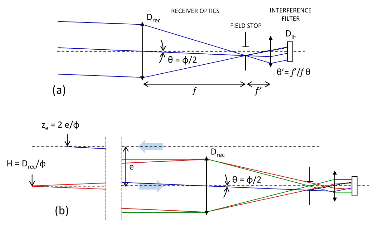
Figure 1 (a) Definition of useful parameters for field angle θ and filter angle of incidence θ^′ calculations. f: receiver focal length; D_rec: receiver diameter; ϕ: full lidar field of view; f^′: collimation focal length; D_IF: IF diameter. (b) Definition of metrics for overlap calculations. e: emitter–receiver separation; H: hyperfocal distance; z_e: entry distance of laser into field of view. Green, red, and blue lines represent rays from infinity, finite distance, and offset emitted beams, respectively.

As previously explained, the impact of deviations on variables in Eq. (15) remains tolerable below a few percent, but for the distinctly more constrained temperature retrieval, the variables in Eq. (16) are affected by the following effects that directly induce significant bias.

• Laser wavelength drift or filter central wavelength (CWL) drift with temperature both affect the ratios indiscriminately with range. By simulating the variation in Q with the WALI filter parameters (Sect. 3), we find a large impact of a wavelength drift Δλ (measured between the laser on one side and both interference filters on the other side): $\mathrm{d}Q/Q/\mathrm{d}\mathit{\lambda }\approx -\mathrm{0.26}{\mathrm{pm}}^{-\mathrm{1}}$ and $\mathrm{\Delta }T\approx -\mathrm{0.34}{}^{\circ }\mathrm{C}{\mathrm{pm}}^{-\mathrm{1}}\mathrm{\Delta }\mathit{\lambda }$, meaning just 3 pm of drift in either filter or laser wavelengths can lead to biases above 1 ^∘C. That is one of the reasons why the laser must be frequency-stabilized. Also, IFs subjected to fluctuations of local temperature are known to experience CWL drifts; for WALI's filters manufactured by Materion, this amounts to 1.28 $\mathrm{pm}{}^{\circ }{\mathrm{C}}^{-\mathrm{1}}$ (value given by the manufacturer after their material dilation simulation). The temperature of the polychromator must thus be kept stable within 1 ^∘C for this bias to become negligible.

• Filter CWL variation with angle of incidence (AOI) on the IF generates a channel transmittance variation which is range dependent and different for each filter. Indeed, this variation ΔCWL is approached by (e.g., Hayden Smith and Smith, 1990)

  $$\begin{array}{}\text{(17)}& {\displaystyle }{\displaystyle }\mathrm{\Delta }\text{CWL}\left({\mathit{\theta }}^{\prime }\right)\approx \text{CWL}{\displaystyle \frac{{{\mathit{\theta }}^{\prime }}^{\mathrm{2}}}{\mathrm{2}{n}_{\text{eff}}^{\mathrm{2}}}},\end{array}$$

  where CWL is the filter central wavelength, θ^′ is the angle of incidence on the filter (assumed small), and n_eff is the effective refractive index of the filter. For the RR1 filter (n_eff=1.62), we obtain as much as $\mathrm{\Delta }\mathrm{CWL}\left({\mathit{\theta }}^{\prime }\right)\approx \mathrm{43}\mathrm{pm}{\mathit{\theta }}^{\prime }$ (^∘)². The problem stems from the fact that because the filter is in the pupil plane, after collimation of the received beam, each angle of incidence corresponds to a different point in the focal plane of the receiver, which in turns corresponds to a field angle θ of the lidar, as seen in Fig. 1a. Aperture number conservation across the receiving optical system imposes

  $$\begin{array}{}\text{(18)}& {\displaystyle }{\displaystyle }{\mathit{\theta }}^{\prime }={\displaystyle \frac{f}{f^{\prime }}}\mathit{\theta }>{\displaystyle \frac{D_{\text{rec}}}{D_{\text{IF}}}}\mathit{\theta },\end{array}$$

  where f and f^′ are the receiver and recollimation focal lengths, and D_rec and D_IF are the receiver and IF diameters. For a 150 mm diameter receiver using a 1 in. diameter (22 mm clear aperture) IF, we obtain at least ${\mathit{\theta }}^{\prime }=\mathrm{0.39}$^∘ for a θ=1 mrad field angle, producing $\mathrm{\Delta }\text{CWL}\left({\mathit{\theta }}^{\prime }\right)\approx \mathrm{6.6}\mathrm{pm}$ and already $\mathrm{\Delta }T\approx \mathrm{2.2}{}^{\circ }\mathrm{C}$. Note that the impact gets proportionately larger with the diameter of the receiver. Because the optical path of each channel is independently aligned, this always induces different overlap factors even when sharing the same telescope. This large effect must be calibrated and corrected, yet its impact was never discussed before in the RR lidar literature, despite being 3 times as large in other systems with 450 mm receivers. This impact can be mitigated by attacking the filters at normal incidence, where the derivative of CWL as a function of AOI (see Eq. 17) is minimal.

• Detector response non-uniformity up to ±12 %, as a function of both impact point on the active surface and angle of incidence, is now specified on the cathodes of PMTs used at the 400 nm wavelength (Hamamatsu, 2007, Sect. 4.3.3). The amplitude was found to be much larger by Simeonov et al. (1999), with a significant impact. This effect has been bluntly limited in all our lidars by putting the cathode plane as far as possible before the focal plane, while still avoiding vignetting. It can still be responsible for differences of overlap factors between channels.

• Uncalibrated PMT gain or digitizer baseline variations will of course induce bias in the channel system constants. We will see how to mitigate these effects.

• Slight variations in overlap or channel transmittance after calibration will be directly responsible for bias. In the next sub-section, we discuss how they can appear.

2.4 Overlap measurement with horizontal shots and limitations

Range-dependent biases influence the lower part of the lidar profiles exactly like the overlap factors. They significantly impact the profiles up to a given range from the emitter, depending on the characteristics of the receiving optics as seen above, but also on the quality of the alignments, which is seldom the same twice. Two methods are used in the literature to approximate the actual overlap factors of a Raman lidar: (i) an iterative Klett inversion of elastic and Raman channels sharing the same telescope is easy to achieve (Wandinger and Ansmann, 2002) but inefficient when non-common-path errors are involved, whereas (ii) the method of aiming the lidar horizontally (e.g., Sicard et al., 2002; Chazette and Totems, 2017) is sometimes impractical but more direct and yields more accurate results in a horizontally homogeneous atmosphere over a range of 1 to 2 km. In the context of RR measurements, it is necessary to implement the latter and also to measure the ratios of overlap factors, rather than the overlap factors themselves, thus avoiding errors due to an imprecise estimation of atmospheric extinction.

Considering a horizontal line of sight in a supposedly homogeneous atmosphere, the expected values of ratios R and Q can be expressed as

$$\begin{array}{}\text{(19)}& {\displaystyle }& {\displaystyle }\stackrel{\mathrm{‾}}{R\left(z\right)}=R\left(z_{\mathrm{\infty }}\right){\displaystyle \frac{O_{{\mathrm{H}}_{\mathrm{2}}\mathrm{O}}\left(z\right)}{O_{{\mathrm{N}}_{\mathrm{2}}}\left(z\right)}}\exp \left(-\mathrm{\Delta }\mathit{\alpha }\cdot z\right),\text{(20)}& {\displaystyle }& {\displaystyle }\stackrel{\mathrm{‾}}{Q\left(z\right)}=Q\left(z_{\mathrm{\infty }}\right){\displaystyle \frac{O_{\text{RR}\mathrm{2}}\left(z\right)}{O_{\text{RR}\mathrm{1}}\left(z\right)}},\end{array}$$

where R(z_∞) and Q(z_∞) are the values observed when all overlap factors have become constant at a sufficiently large range from the lidar, noted as z_∞, after which variations in the optical path inside the reception channels become negligible. $\mathrm{\Delta }\mathit{\alpha }=\mathit{\alpha }\left(\mathrm{407}\mathrm{nm}\right)-\mathit{\alpha }\left(\mathrm{387}\mathrm{nm}\right)$ is the difference of atmospheric extinction between the two VR wavelengths.

To evaluate z_∞, in Fig. 1b we introduce parameters that characterize the overlap of a paraxial or coaxial lidar (e.g., Kuze et al., 1998): (i) $z_{\mathrm{e}}=\mathrm{2}e/\mathit{\varphi }$, at which the emitted laser beam located at distance e from the receiver axis enters the field of view, whose full size is ϕ, and z_e is null for a coaxial system; (ii) $H=D_{\text{rec}}/\mathit{\varphi }$, the so-called hyperfocal distance, the minimum range from which the beam originating from a point still fully enters the field stop; (iii) $H_{\text{IF}}=\mathrm{2}{D}_{\text{rec}}f/f^{\prime }{{\mathit{\theta }}^{\prime }}_{\text{max}}$, which we might call the filter hyperfocal distance, similarly to the former, the minimum range from which the image of a point does not exceed ${\mathit{\theta }}_{\text{max}}^{\prime }$, the AOI on the IF that significantly changes its transmittance. z_∞ is above the maximum of those three, which is usually H_IF. If we use for ${\mathit{\theta }}_{\text{max}}^{\prime }$ the AOI value causing 1 ^∘C bias on temperature in Eqs. (10) and (15), we find $z_{\mathrm{\infty }}>H_{\text{IF}}=\mathrm{780}$ m. Note that z_∞ can reach several kilometers with misaligned filters.

If for instance the lidar can be mounted on a rotating platform capable of aiming horizontally, the overlap ratios ${\text{OR}}_R\left(z\right)=O_{{\mathrm{H}}_{\mathrm{2}}\mathrm{O}}\left(z\right)/O_{{\mathrm{N}}_{\mathrm{2}}}\left(z\right)$ and ${\text{OR}}_Q\left(z\right)=O_{\text{RR}\mathrm{2}}\left(z\right)/O_{\text{RR}\mathrm{1}}\left(z\right)$ can be estimated with suitable precision ($\sim {\mathrm{10}}^{-\mathrm{3}}$) by averaging the signals over time, smoothing them over range, and finally correcting for the differential of extinction on the VR ratio:

$$\begin{array}{}\text{(21)}& {\displaystyle }& {\displaystyle }\widehat{{\text{OR}}_R}\left(z\right)={\displaystyle \frac{R\left(z\right)}{R\left(z_{\mathrm{\infty }}\right)}}\exp \left(\mathrm{\Delta }\mathit{\alpha }\cdot z\right),\text{(22)}& {\displaystyle }& {\displaystyle }\widehat{{\text{OR}}_Q}\left(z\right)={\displaystyle \frac{Q\left(z\right)}{Q\left(z_{\mathrm{\infty }}\right)}}.\end{array}$$

These estimates of the overlap ratios will then be used during signal processing for vertical shots as in Eqs. (4) and (5). However, assumptions are made for the former estimation, namely the following.

• As explained above, the atmosphere is assumed to be homogeneous in WVMR and temperature (down to <0.5 ^∘C) up until z_∞, whereas the overlap ratios must be constant (down to <0.4 %) after z_∞. Also, the maximum range (with sufficient SNR) of the lidar must exceed z_∞, implying nighttime measurements for the Raman channels. Therefore, the effects generating overlap variation after a few hundred meters must be prevented.

• The lidar is assumed to retain the exact same overlap functions when aiming horizontally and vertically. Considering a field of view around 1 mrad, the stability of the emission and reception optical paths must be better than ∼10 µrad between these two positions. This is feasible for a small refractor but difficult for a Raman system such as WALI, with a heavy laser and large reflector.

These difficulties make it extremely challenging to estimate the overlap ratios with an accuracy better than a few percent. This is enough for the WVMR, but we find that a correction must be applied by comparing with in situ sounding for temperature measurements by Raman lidar.

3 Implementation and bias mitigation on the WALI system

In this section, we describe the WALI instrument from the emitter to the reception channels, characterizing the critical elements in the framework of WVMR and temperature measurements. The system has evolved from its previous implementation described in Totems et al. (2019), by adding RR channels and a fibered telescope receiver. A global diagram presenting the main lidar sub-systems is shown in Fig. 2, and a summary of its characteristics is given in Table 2.

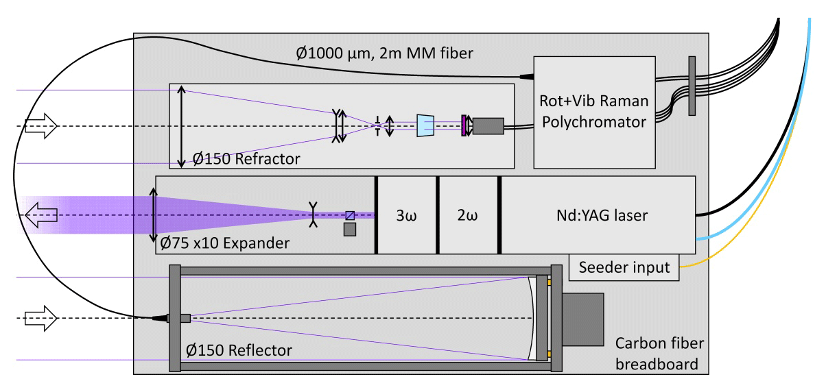
Figure 2 Global diagram of the lidar system. The main sub-systems are the emitter (center), the elastic receiver using a refractor (top), the Raman receiver using a fibered parabolic reflector (bottom), and a separate, thermally stabilized polychromator (upper right). See Fig. 5 for the detail of the polychromator design.

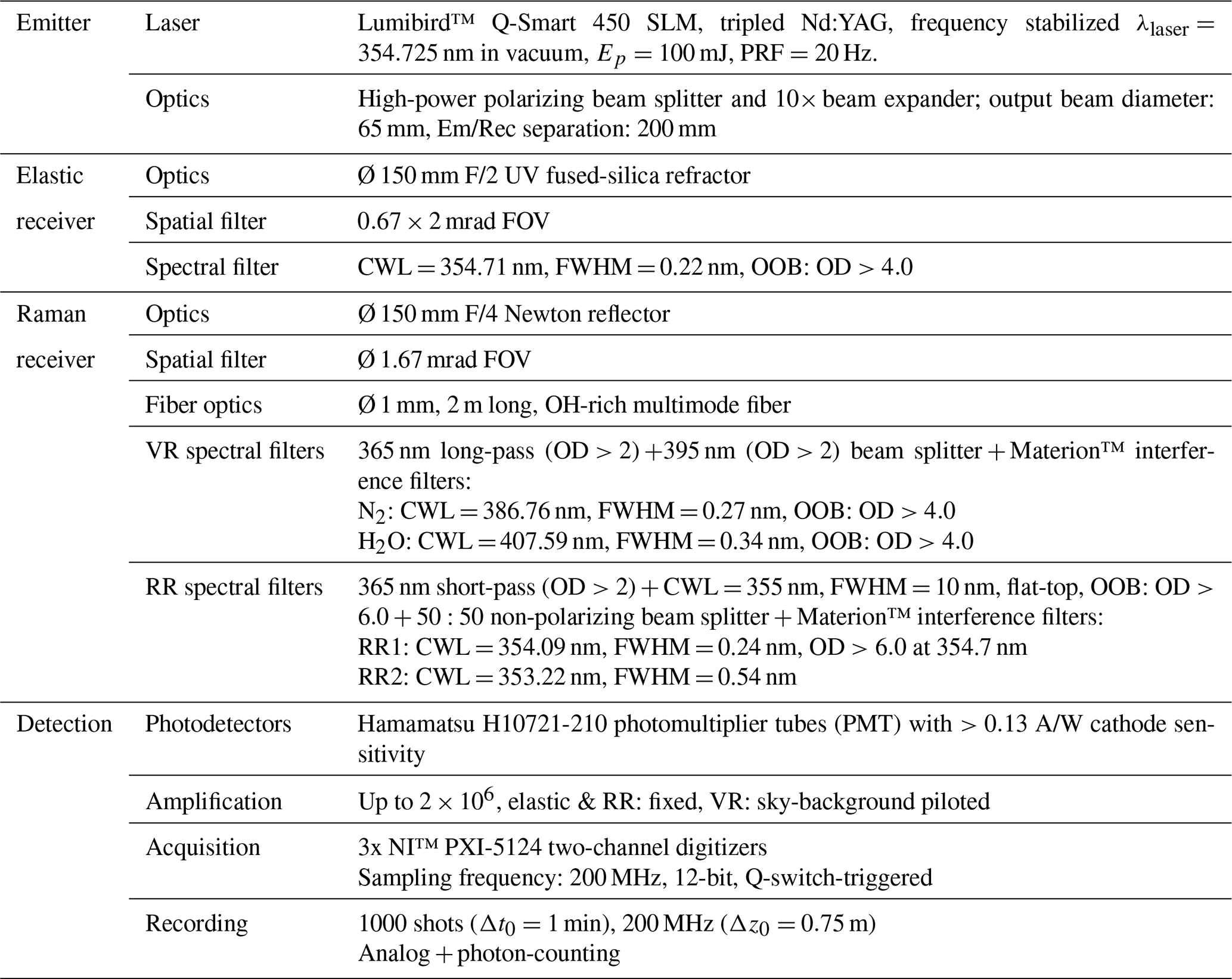
Table 2 WALI instrument characteristics summary (PRF: pulse repetition frequency; FOV: field of view; CWL: central wavelength in vacuum; FWHM: full width at half maximum; OOB: out-of-band blocking specification; OD: optical density).

Its main features are a single rotatable platform (lightweight carbon fiber breadboard by CarbonVision GmbH) carrying both its emission and reception paths, a 150 mm refractor for the elastic channels (for aerosol studies), and a 150 mm diameter parabolic fibered reflector for all the Raman channels. The separation of the four Raman channels takes place in a deported polychromator set in a thermally controlled enclosure, fed by the optical fiber. Fiber optics are also known to partly scramble the input illumination, which could help minimize the range dependance of filter transmittance or detector sensitivity for the different Raman channels. The output signals from the photomultiplier tubes (PMTs) in the polychromator are digitized by a NI™ PXI system (not shown).

3.1 Emitter

The emitter is a commercial Lumibird/Quantel “Q-Smart 450” Nd:YAG pulsed laser, stabilized by injecting the output of a single longitudinal mode fiber laser emitting at 1064.175 nm into the main cavity (“SLM” option) and frequency-tripled to emit at wavelength λ_laser=354.725 nm (in vacuum). The nominal pulse energy for the Q-Smart 450 with SLM is 100 mJ at 355 nm, with a pulse repetition frequency (PRF) of 20 Hz. These values set WALI near the eye safety limit for pulsed energy, making the system eyesafe at the output of a 2 m funnel, as limited by leaks at 532 nm through the built-in filtering dichroic plates.

A critical issue to be cleared before using the Q-Smart 450 SLM in WALI was the spectral purity and stability of the laser, in terms of line width and wavelength drift. The laser seeder at 1064.175 nm is specified with a 50 MHz (0.062 pm at 355 nm) stability at fixed temperature and 37 $\mathrm{MHz}{}^{\circ }{\mathrm{C}}^{-\mathrm{1}}$ (0.046 $\mathrm{pm}{}^{\circ }{\mathrm{C}}^{-\mathrm{1}}$ at 355 nm) temperature drift.

Nevertheless, the stability of the Q-Smart emission at 354.725 nm has been verified with a dedicated optical setup, sending the output of a Michelson interferometer with optical path differences (OPDs) between 0 and 100 mm on a UV-sensitive CCD camera. By extracting the contrast and phase variations in the fringes at large OPDs from the videos, we were able to ascertain

• the laser line width, without seeder to be 24±2 pm (versus 26.5 pm data sheet value), and with seeder, to be small compared to 1 pm (versus 0.2 pm data sheet value);

• the wavelength drift, without seeder to be below 8 pm over 10 min, and with seeder, to be below 0.2 pm rms (root-mean-square fluctuations) over 5 min. We consider the remaining fluctuations to be mostly due to the ∼0.05 $\mathrm{pm}{}^{\circ }{\mathrm{C}}^{-\mathrm{1}}$ temperature-linked drift of the seeder, which is not temperature-controlled and was recently turned on.

Given the requirements derived in Sect. 2.3, this makes the seeded Q-Smart laser theoretically suitable for RR measurements of temperature.

3.2 Raman receiver

In this sub-section we discuss the possible impact on the VR$/$RR ratios of the fibered reflector (beam scrambling and fiber optics fluorescence), of Raman filters characteristics, and of the polychromator design and alignment. As far as we know, this type of comprehensive study does not exist in the literature for Raman lidars.

3.2.1 Fibered reflector telescope and scrambling of the lidar field of view

The elastic and Raman receivers are both 150 mm in diameter. The focal length of the refractor (elastic channels) is ∼300 mm, which with a 200×600 µm field stop achieves full overlap at ∼150–200 m. However, the focal length of the reflector (Raman channels) is 600 mm (parabolic mirror with aperture F/4); this implies using a multimode fiber optics about 1 mm in diameter as the field stop to allow similar results in terms of field of view and overlap. The chosen fiber optics is an OH-rich UV fused-silica fiber, 2 m in length and 1000 µm in core diameter, with a numerical aperture of 0.22 (Avantes FC-UV1000-2).

Coupling the reflector output into a multimode fiber (e.g., Chourdakis et al., 2002) allows us (i) to minimize occultation of the primary mirror (here only 12 mm in diameter); (ii) to deport the Raman channel separation away from the telescope, making it a separately tunable optical system, minimizing the overall lidar size and making light or temperature confinement easier; and (iii) in theory, to scramble the fiber output illumination versus the lidar field angle, therefore minimizing the range dependence of AOIs on the IFs discussed in Sect. 2.3 and flattening overlap ratios after the geometrical full-overlap distance.

The scrambling of the lidar field of view, via the multiple internal reflections in the fiber, has been experimentally tested by imaging the output of the fiber, with a varying point-like input. The results are shown in Fig. 3. Note that the radial coordinate of the output point relative to the center of the fiber corresponds to a given AOI on a well-aligned IF in the following polychromator, after a $f^{\prime }=\mathrm{50}$ mm doublet lens.

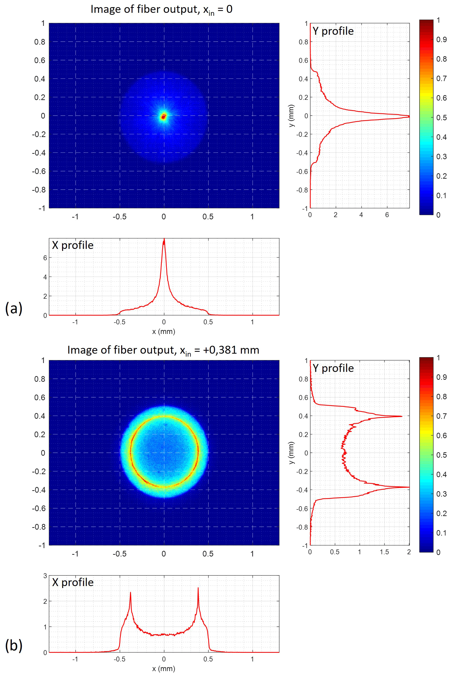
Figure 3 Images of the output facet of the 1 mm diameter multimode fiber optics for (a) centered and (b) decentered (at x_in=0.38 mm horizontal offset from the center of the core) input point of a 20 mm beam focused on the input facet of the fiber and energy density profiles along the x and y axes.

It appears in Fig. 3b that the input energy is mostly redistributed tangentially (i.e., along the angular polar coordinate, as opposed to radially) by its passage through the fiber. The radial dispersion remains small, and the mean output radius is approximately equal to the input radial coordinate. Manually applying curvature to the fiber, as suggested by so-called “mode scrambling” devices, did not make the energy distribution more uniform so much as creating unwanted losses (effect not shown). Even for a centered input, the energy radial distribution – i.e., the percentage of the total output in a given radial bin, which will therefore impact a well-aligned filter at the same AOI – is uniform. We conclude that even with the use of fiber optics the angle of incidence on the interference filters depends on the image positions in the focal plane of the telescope (i.e., mainly the distance to the optical axis), in contrast to what could be expected. Range-dependent biases will not be strongly mitigated.

3.2.2 Fiber optic fluorescence

It has been shown by Sherlock et al. (1999) and discussed by Whiteman et al. (2012) that fiber optics fluorescence could be an obstacle to water vapor measurements, because elastic scattering at 532 nm was inducing fluorescence in an OH-poor fiber at a non-negligible level compared to the atmospheric Raman scattering. It was solved by using an OH-rich fiber, but it was predicted in the latter work that the effect could be larger at 355 nm.

We have characterized this effect in the WALI fiber optics, using a narrowband CW laser excitation centered at 355 nm. The output of the fiber was analyzed by a Fourier transform spectrometer (Thorlabs OSA201C spectrum analyzer), behind a long-pass dichroic plate cutting the direct laser emission, and the same collimating achromat as in the polychromator. The resulting spectrum is shown in Fig. 4.

Figure 4 The 1000 µm diameter, 2 m long fiber fluorescence measurement with 355 nm laser illumination.

We plot both the raw spectrum and the Fourier transform spectrometer noise floor after 1000 profile integrations, to highlight the very weak features observed at 780 to 910 nm and the high associated uncertainty. Due to the noise level, and given the dichroic plate residual transmittance of the laser wavelength, we can only ascertain that the fluorescence power spectral density (PSD) around 400 nm is lower than 10⁻⁶ times the peak laser PSD, although no feature can be detected in this spectral domain. Note that fluorescence between 400 and 500 nm was indeed observed using a broadband excitation from a fibered LED at 340 nm (not shown). Nevertheless, the amount of rejection observed for a 355 nm excitation is sufficient to exclude an adverse impact of the OH-rich fiber optics for Raman lidar measurements.

3.3 Raman channels

3.3.1 Polychromator configuration

The RR + VR polychromator configuration used in WALI is presented in Fig. 5. Dichroic and non-polarizing beam splitters are used to separate the channels. In contrast to the design of Hammann et al. (2015) which optimizes throughput and laser-line rejection on the RR channels, we chose to implement a splitter-based configuration, favoring a compact system (25×25 cm, easier to confine) and normal incidence on the filter, at the expense of SNR. Indeed, designing the filters for a correct CWL at 5^∘ incidence (as in the cited work) instead of 0^∘ dramatically narrows the filter angular acceptance, as can be deduced by deriving Eq. (15) as a function of incidence θ^′. In the WALI polychromator, the output from the fiber is collimated by a near-UV achromat with 50 mm focal length, resulting in a 22 mm diameter beam. Dichroic beam splitters with adequate cut-on wavelengths are used to separate channels. On each separated channel, an aspheric lense condenses light on the PMT surface, located 4 mm before the focal plane. A steel cage system assembly holds all parts with great stability; however beam splitters are not always perfectly aligned at 45^∘ in the stock cage cubes. That is why all filter, lens, and PMT sub-assemblies are mounted on tiltable mounts to allow precise alignment at normal incidence.

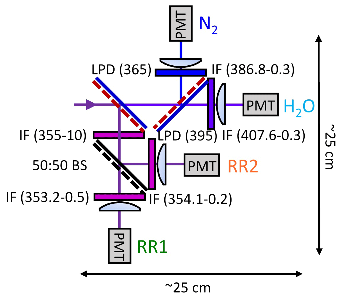
Figure 5 Compact rotational and vibrational Raman separation configuration used in WALI. IF: interference filter (with CWL–FWHM given in nanometers); BS: beam splitter; LPD: long-pass dichroic beam splitter (with cut-off wavelength given in nanometers); PMT: photo-multiplier tube. This polychromator is thermally regulated in a dedicated light-tight enclosure.

3.3.2 Filter qualification

All interference filters were custom-made by Materion, including the RR filters on specifications graciously shared by the team of A. Behrendt (following Hamann et al., 2015). They were characterized on the Fourier transform spectrometer (described in Sect. 3.2.2) prior to mounting, using fibered LEDs peaking at 340, 385, and 405 nm as the light source; the beam was collimated by the same near-UV achromat with 50 mm focal length. We give the measurement results for the RR filters in Fig. 6 and Table 3.

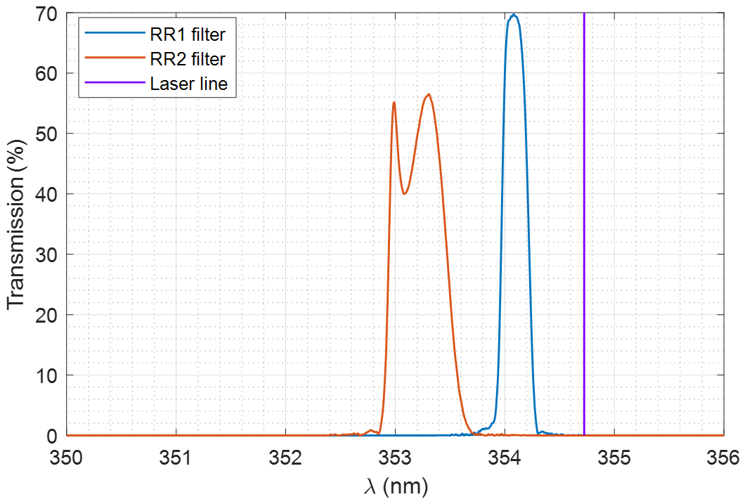
Figure 6 RR filter spectral transmittance measured with an optical spectrum analyzer with illumination by a 340 nm LED: RR1 (low-J) and RR2 (high-J) filter at 0^∘ incidence.

Table 3 Measured RR IF characteristics. All CWL values are given in vacuum.

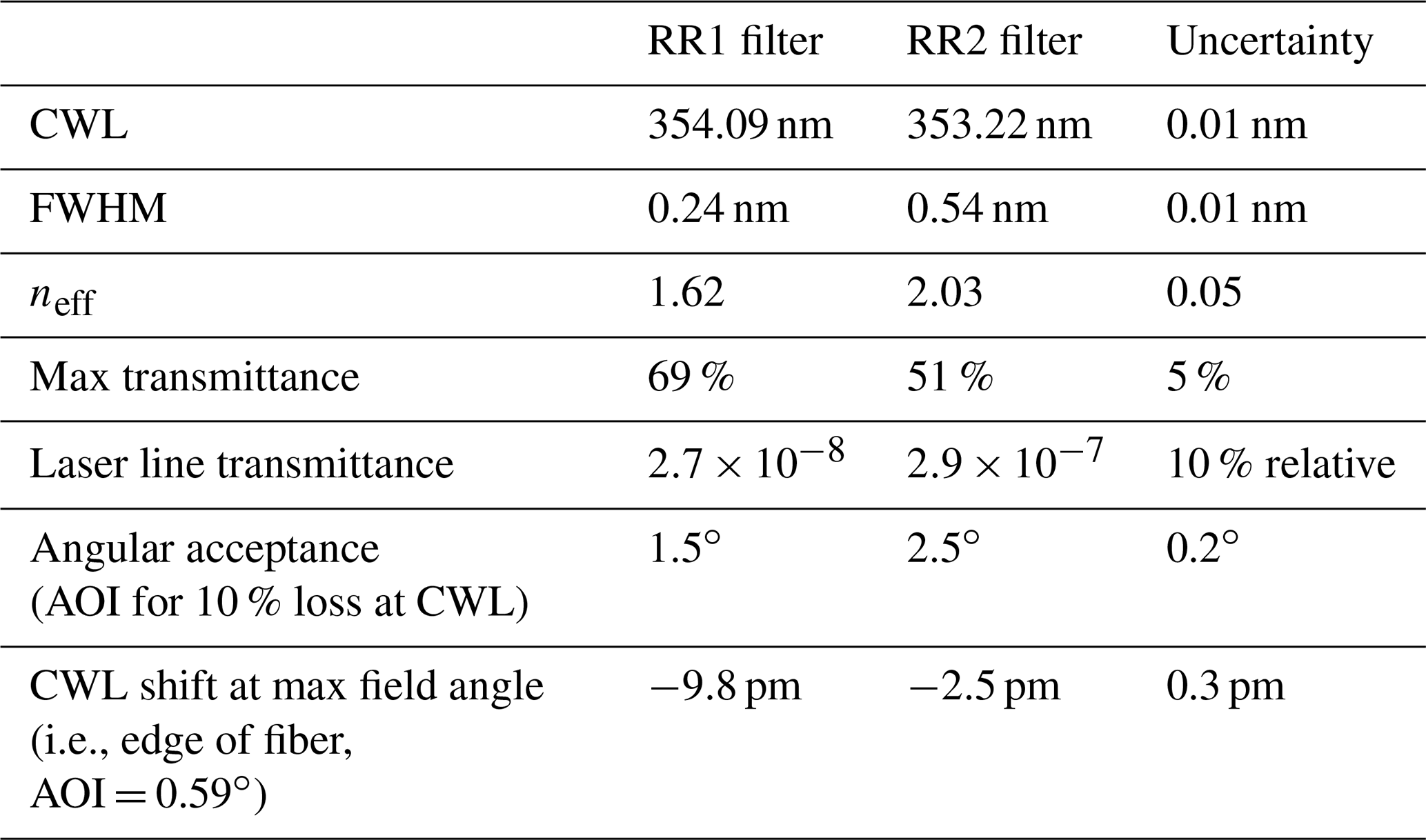
The effective index and angular acceptance of the filters (arbitrarily chosen for a 10 % loss at the CWL) were assessed by tilting the filters of a known angle. A critical parameter, the transmittance of both filters at the laser line λ_laser in operational conditions, was assessed on the lidar itself, by measuring the energy of an echo on a hard target located at 200 m and switching between an elastic IF of known transmittance with a known strong optical density and the RR IF in question. The excellent extinction in the RR1 filter guarantees a minimal effect of elastic signal leak in temperature retrievals, but it was nevertheless subtracted as in Eq. (3). Note that no significant echo was detected on the H₂O-Raman channel, indicating extinction better than a few 10⁻⁹, thanks to the two dichroic plates.

3.3.3 Polychromator alignment and qualification

Due to the filter CWL shift evolving as the square of the AOI in Eq. (15), it is essential to minimize range-dependent biases by aligning the filters at a precisely normal incidence from the input beam. However off-the-shelf beam splitter plate holders are found to be misaligned by up to 1^∘ from an ideal 45^∘ incidence. All PMTs are mounted jointly with their own IF and lens into a tiltable mount to correct for this (represented in Fig. 7).

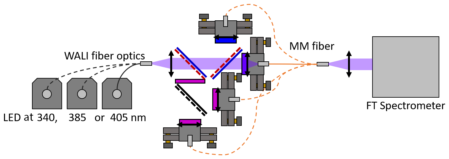
Figure 7 Method for polychromator alignment validation. Light from LEDs is input in the WALI fiber optics and passes through the polychromator and into a multi-mode fiber (MM fiber, Ø 600 µm) analyzed by a Thorlabs OSA201C Fourier transform spectrometer. Central channel wavelengths are expected not deviate from those of the filter measured independently at normal incidence, to validate alignment.

The alignment of these mounts is performed in the lab by conjugating an input multimode fiber of 600 µm diameter replacing the lidar input, into a target fiber 200 µm in diameter at the focus of the PMT lens, through the polychromator. Fibered LEDs are used for illumination like in Sect. 3.3.2. All the channels are sequentially addressed in this manner. By obtaining a maximal energy and a radially uniform profile at the output of the target fiber, one can ensure alignment with a precision of 0.1 to 0.3^∘.

To verify the result, the spectral transmittance of the polychromator channels themselves are characterized by the Fourier transform spectrometer, as shown in Fig. 7. By illuminating the channel with a LED coupled in the actual lidar fiber, we ensure that the polychromator is studied in operational conditions. The CWL of each channel is expected not to deviate by more than 20 pm (twice the empirical accuracy) from the CWL measured on the individual filter at normal incidence, to validate the alignment. The polychromator aligned using the procedure proposed above passes this test.

3.4 Detectors

Hamamatsu 10721P-210 PMTs, with >0.13 A W⁻¹ cathode sensitivity at 400 nm, and up to $\sim \mathrm{2}\times {\mathrm{10}}^{\mathrm{6}}$ controllable internal gain, are used to transform the optical flux into an electric current, directly digitized at 200 MHz (0.75 m sampling along the line of sight) by three NI PXI-5124 two-channel digitizers with 50 Ω load. The acquisition software, custom-made with LabVIEW, conducts analog and photon-counting (thresholding at ∼3 standard deviations of the noise) accumulations in parallel during 1000 shots (50 s), every minute, which are then pre-processed and recorded (∼10 s downtime). Every ∼8 min, baselines are recorded with PMT gains set at zero. The next sub-sections describe critical points of the detectors affecting the RR and VR channel ratios.

3.4.1 PMT response variability

As explained in Sect. 2.3, the non-uniformity of the PMT response can affect the ratios of Raman channels as a function of range. We tested the sensitivity profiles of WALI's H₂O-Raman PMT to continuous laser illumination at the 405 nm wavelength, first using a 1 mm diameter collimated beam, as a function of both point and angle of incidence. A cumulated ∼6.0 neutral density filter was used to avoid saturation of the PMT.

As shown in Fig. 8a, a strong variation in sensitivity by a factor of almost 2 is found on the PMT surface, much larger than specified. The relative sensitivity is lowest near the center of the PMT and highest on the sides, at a diameter of 4 mm approximately equal to the spot size in the lidar. Indeed the PMT surface is 4 mm before the focal plane of the 0.5 NA condensing aspheric lens. This is consistent with the results of Simeonov et al. (1999) on an older generation of detectors, excluding a suspected hole-burning phenomenon over the lifetime of our PMT. On the vertical axis, we also note the effect of the gridded cathode. Note that sensitivity does not vary by more than a few percent as a function of angle of incidence (not shown).

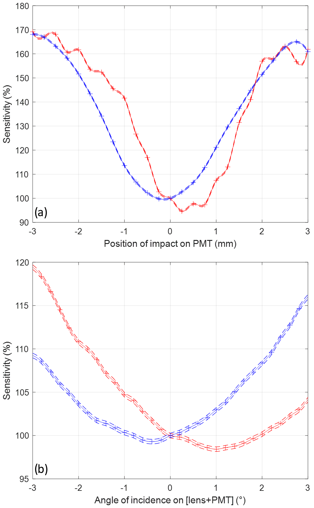
Figure 8 Study of the non-uniformity of the PMT response: (a) as a function of point of impact on the active area along the horizontal (blue) and vertical (red), with a 1 mm collimated beam from a 405 nm laser, and (b) as a function of angle of incidence on the lens and PMT assembly similar to the ones used in the WALI polychromator, with a 22 mm collimated beam from the same laser. Dashed lines represent uncertainty calculated over multiple measurements. Sensitivity is given normalized by its value at the approximate mechanical center of the PMT or at normal incidence as determined using the reflection on the attached neutral density filter.

We then put the condensing lens used in the polychromator in front of the PMT and studied its response as a function of AOI on the lens + PMT assembly, which is shown in Fig. 8b. The input beam was the nominal size in the polychromator, i.e. ∼22 mm in diameter. We find that the curve corresponds well to the measured sensitivity profile, smoothed by its convolution with the spot on the PMT. The problem is that at normal incidence, the derivative of sensitivity with incidence is 2 %–5 % per degree. Using the calculations in Sect. 2, a θ=1 mrad field angle corresponds to 0.39^∘ incidence on the PMT, inducing potentially 0.8 %–2 % bias on R and Q and thus a significant 1 to 2 ^∘C bias on temperature. In the future, the condensing lenses will be replaced with afocal beam reducers to reduce this dependency.

3.4.2 Baseline and EM parasite correction

The baseline induced by the detection chain is found to vary between channels and in time. It is also subject to electro-magnetic (EM) interference, causing parasitic signals of both high frequency, mostly due to the strong flashlamp peak current radiating over the system, and low frequency, probably due to other neighboring electronics. For this reason, the channel baselines are evaluated regularly (by averaging 1000 shots with PMT gain set to zero, every 8 min), smoothed and corrected (L_j in Eq. 2). However, for the Raman channels (H₂O and RR2 specifically), the weakness of the signals requires a specific care of EM compatibility, as repeating parasitic spikes were found to jam the channels (especially photon counting, which relies on thresholding) starting at an altitude of 6–7 km.

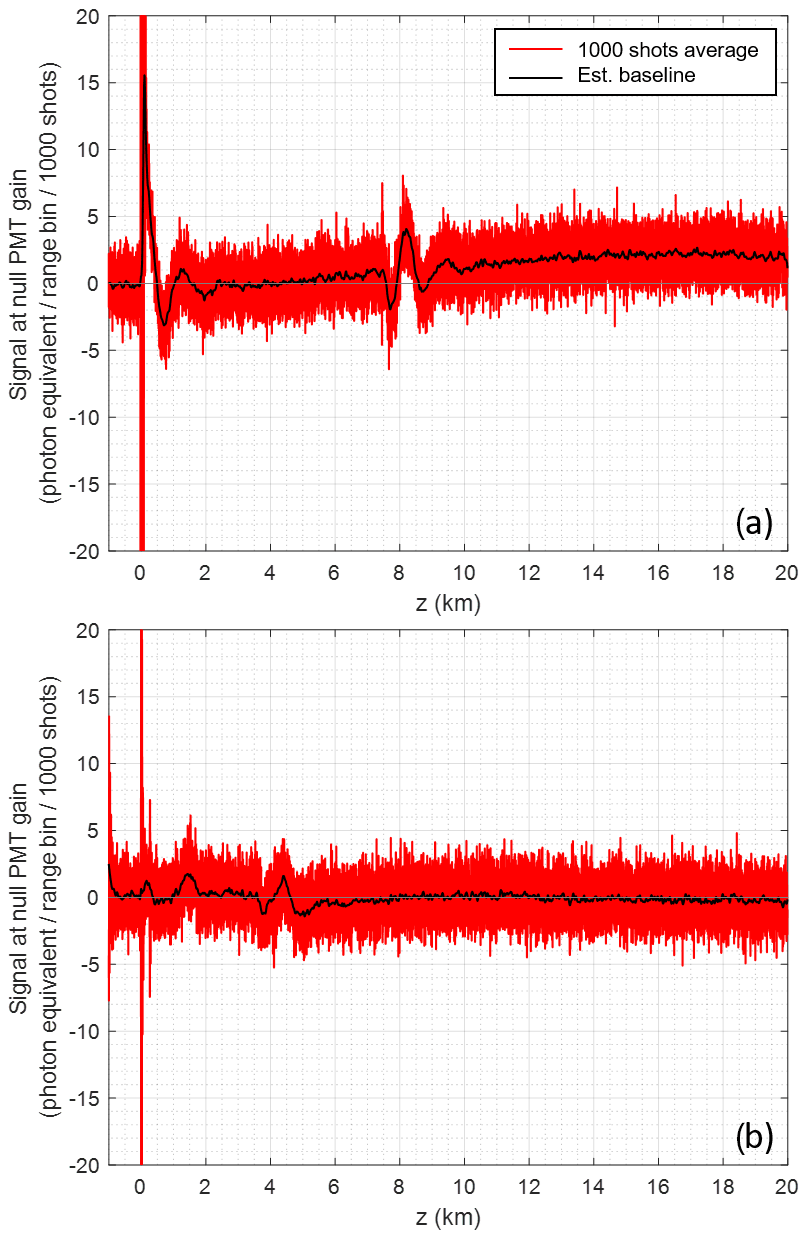
Figure 9 Analog detection baseline measurements (red) over 1000 laser shots with PMT gains set to zero, expressed in photon counts equivalent on the RR2 channel: (a) in an unfavorable case (no mitigation), showing both baseline fluctuations over time (20 km∼133 µs) and strong electro-magnetic parasites at large distance, and (b) on the WALI system, after mitigation. The final estimated baseline (${\widehat{L}}_j\left(z\right)$ in Eq. 3) obtained after smoothing, which is subtracted to all recorded profiles, is in black.

Figure 9a shows an example of perturbed baseline. Trial and error established that common methods to avoid ground loops were not all efficient: star grounding of the various cables worsened the problem, whereas physically separating coaxial signal cables from direct current power supply and control voltage cables, and grounding all connectors and opto-mechanics again on the breadboard side, mitigated it, reaching the baseline plotted in Fig. 9b. Note that baseline variation is not significant between successive evaluations without an external perturbation; the estimated baseline is automatically subtracted from the profiles before recording during the next 8 min (Eq. 3).

3.4.3 PMT gain adaptation

On each channel, PMT internal amplification gain G (using photoelectron multiplication) is a definite function of its control voltage U. The variation in G by ∼2 orders of magnitude allows for the optimization of the dynamic range. This helps deal with the different Raman cross sections in each filter, with variations in atmospheric transmittance, and especially with sky background levels during daytime. The gain is pushed at its maximum possible value still satisfying two conditions: (i) the signal voltage maximum does not exceed the range of the digitizer, and (ii) the sky background signal does not exceed the maximum output current of the PMT that guarantees linearity (100 µA, i.e., 〈S_raw〉<5 mV). This is indispensable for day-round measurements of WVMR, otherwise the channels would be saturated during daytime (Chazette et al., 2014b), or suboptimal in SNR during nighttime.

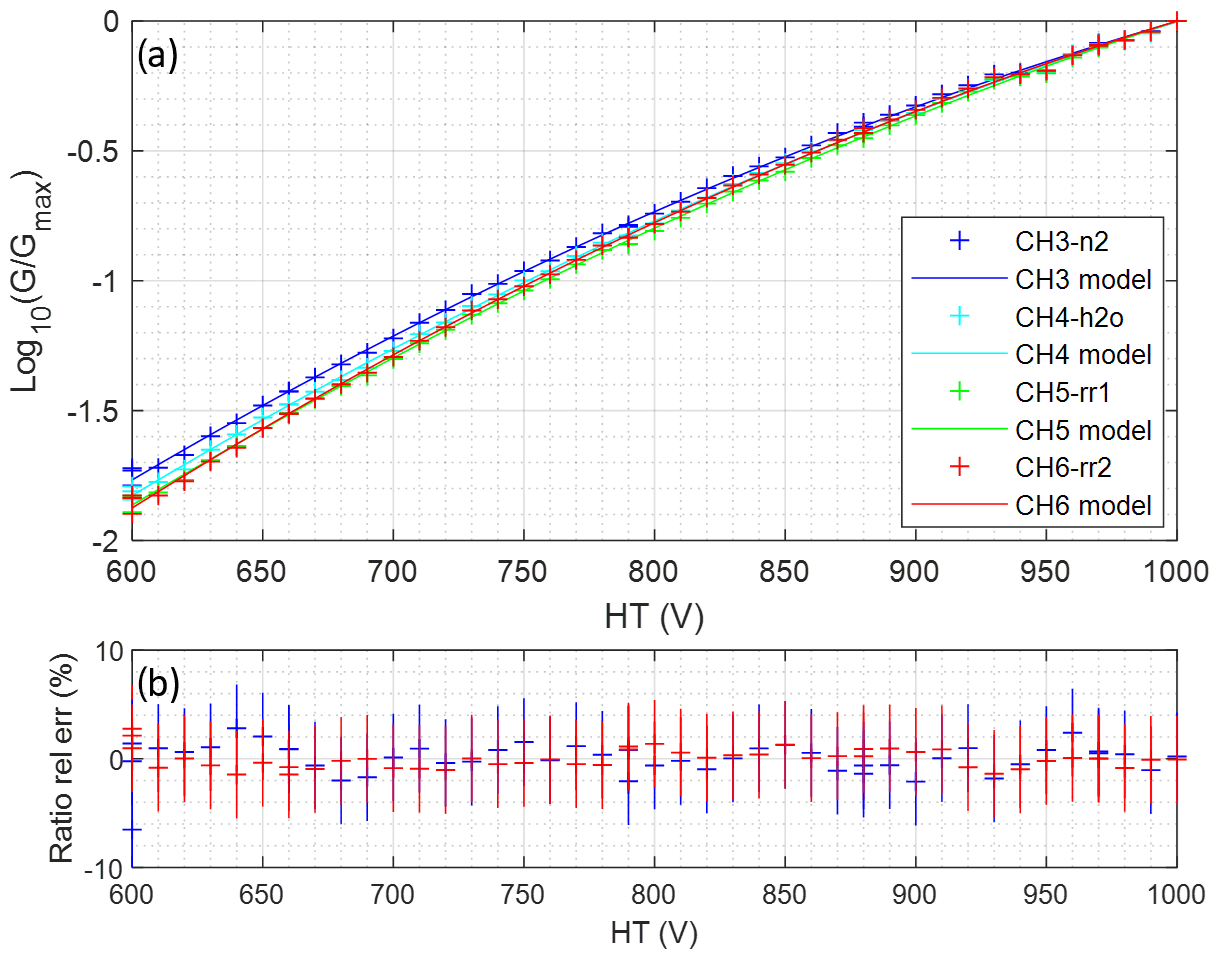
Figure 10 Calibration of PMT gain G versus control voltage U: (a) log-gain measurements and second-degree polynomial model for all Raman channels and (b) relative gain ratio error between model and measurements for vibrational and rotational Raman channel ratios.

However, PMT gain adaptation leads to biases on the Raman channel ratios if the gain versus control voltage characteristics are not known with a better precision than the requirements stated in Table 1 (2 % on VR channels, 0.4 % on RR channels). In Fig. 10a, we show the experimental calibration of G versus U as well as second-degree polynomial fits for each channel. The relative error on the VR and RR channel gain ratios approximated by these models is plotted in Fig. 10b, with the measurement uncertainty. This uncertainty is mostly due to variations in atmospheric parameters and laser energy during calibration. Since all relative errors are well centered, we compute that the possible error for the gain ratio with these models is ∼1.3 %. This is compatible with WVMR measurements but not with temperature measurements. Therefore, the PMT gain should only be adapted on the VR channels, and the RR channels should be kept at a fix value of gain.

3.4.4 Merging analog and photon-counting signals

Both analog and photon-counting raw signals are recorded. The analog signal has lesser SNR at high altitude during nighttime, whereas the photon-counting signal is saturated at low altitude and by daylight; by merging them correctly, an optimal SNR can be obtained (Newsom et al., 2009). For signal processing, the photon-counting raw signals are first desaturated (details in Chazette et al., 2014b). Merging is performed during nighttime on the pre-processed signals defined in Eq. (3). After calculating a photon-to-volt conversion constant at an altitude where photon counting is not saturated, the converted photon-counting profile replaces the analog profile after a predefined altitude depending on signal strength (from 1 km for the H₂O VR channel up to 4 km for the elastic channel).

We wish to emphasize here that baselines L_j and background signals B_j in Eq. (3) must be estimated separately for the analog and photon-counting recorded profiles (which have no baseline and a smaller but non-zero background value due to the suppression of electronic noise). Otherwise, the merged signal will show discontinuities at the cut-off altitude and biases at high altitude at dusk and dawn. Their impacts are typically much larger than the requirements of Sect. 2.2.

4 Qualification on the atmosphere

In this section, we qualify the WALI system starting with the measurement of its overlap factor ratios, followed by its calibration and comparisons with radiosoundings. Remaining biases are highlighted and corrected, and experimental measurement errors are evaluated.

4.1 Experimental set-up and strategy

We put the lidar into operation in our laboratory near Saclay (48^∘42^′42^′′ N, 2^∘08^′54^′′ E) over a period of 2 weeks in May 2020. It was placed on a rotating platform below a trapdoor equipped with silica windows for zenith shots and in front of a window at a height of about 9 m above the ground level (a.g.l.) for horizontal shots. During the latter, the lidar aimed north <5^∘ above the horizon (beam elevation <80 m per kilometer of range). In that direction, land use is fields up to 800 m in range, buildings and trees between 800 and 2 km in range, and fields again up to 5.5 km in range.

To calibrate and qualify the lidar measurements, we use radiosoundings launched two to three times daily from the operational Météo-France station located in Trappes (48^∘46^′27^′′ N, 2^∘00^′35^′′ E), 12.3 km WNW from the lidar near Saclay, approximately upstream in the prevailing winds, although the wind was oriented mostly NE during the May 2020 period.

4.2 Measurement of overlap ratios with horizontal shots

The overlap factors and their ratios were estimated on signals averaged over 3 h after sunset on 19 December 2019, with a tepid (14 ^∘C), non-turbulent but hazy atmosphere (aerosol extinction coefficient 0.32 km⁻¹ at 355 nm with Ångström exponent ∼1.5, 11 ^∘C ground temperature, and WVMR at ground level around 6.5 g kg⁻¹). With a planetary boundary layer (PBL) height of ∼900 to 1000 m, and slow gradients of temperature (−1 to −4 ${}^{\circ }\mathrm{C}{\mathrm{km}}^{-\mathrm{1}}$) and WVMR (−0.8 to −1.2 $\mathrm{g}{\mathrm{kg}}^{-\mathrm{1}}{\mathrm{km}}^{-\mathrm{1}}$) in that PBL (as measured by radiosoundings launched from Trappes at ∼12:00 and 00:00 UTC, presented in the next subsection), conditions were excellent for a homogeneous atmosphere within the first 5 km at least.

The estimated overlap factors of the different channels, with atmospheric extinction fitted between 800 and 2000 m, are shown in Fig. 11a. Full geometrical overlap is obtained as expected between 150 and 200 m, but the curves differ by several percent between the Raman channels. Atmospheric extinction drifts from the estimated value after 2 km.

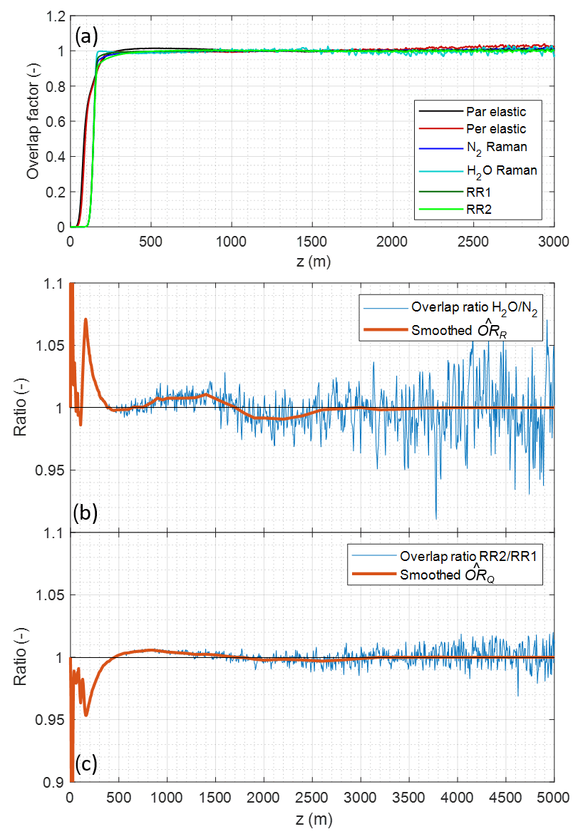
Figure 11 (a) Overlap factors measured over 3 h of nighttime measurements with a horizontal line of sight on 19 December 2019. Estimated overlap ratios between VR (b) and RR (c) channels: native resolution (thin blue line) and final estimate after smoothing (thick red line).

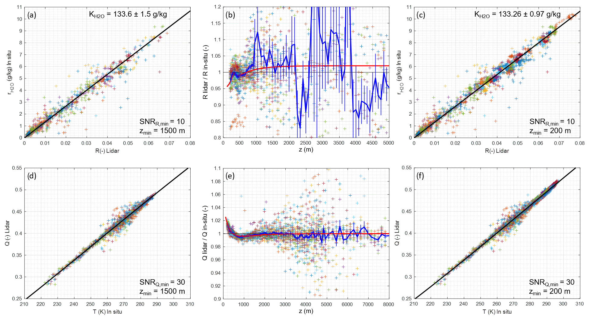
Figure 12 Results of calibration on 12 nighttime and 24 daytime radiosoundings launched from Trappes between 20 May and 2 June 2020 for WVMR (a–c) and temperature (d–f), in three steps: calibration on measurements above 1500 m (a, d) with samples as crosses (one color per radiosonde) and calibration curve in black; residual overlap ratio estimation (b, e) with samples as crosses, mean ratio in blue, random error on mean ratio as vertical bars, and model in red; and calibration on all results (c, f). Daytime samples are limited to SNRs above 10 for R^′ (WVMR) and 30 for Q^′ (temperature).

The estimated ratios of overlap factors OR_R and OR_Q are plotted in Fig. 11b and c, at 7.5 m resolution (thin line) and after smoothing (thick line, final correction used hereafter). Peak divergence is 5 % to 7 %, at ∼150 m. Convergence within 1 % happens at ∼400 m, but oscillations of lower amplitude persist until ∼3 km. We note that for OR_Q, deviations do not exceed the ±0.7 % required to maintain bias below 1 ^∘C. They are nevertheless corrected.

4.3 Comparison to radiosoundings and calibration, estimation of residual error

In total 12 nighttime and 24 daytime radiosoundings were launched from Trappes between 20 May and 2 June 2020. Lidar profiles are averaged from 0 to 40 min after the radiosounding launch time. The range averaging is progressive and defined to keep the nighttime temperature error below 1.5 ^∘C: range bins are 15 m long below 100 $\mathrm{m}\mathrm{a}.\mathrm{g}.\mathrm{l}.$, growing to 360 m above 8 $\mathrm{km}\mathrm{a}.\mathrm{g}.\mathrm{l}.$

In order to de-bias WVMR and temperature measurements from residual errors on OR_R and OR_Q, we perform a three-step calibration.

• In the first step, we exclude the first 1500 $\mathrm{m}\mathrm{a}.\mathrm{g}.\mathrm{l}.$ of the profiles when fitting $r_{{\mathrm{H}}_{\mathrm{2}}\mathrm{O}}$ in situ vs. R^′ and Q^′ vs. T in situ to estimate K and f, respectively. This initial calibration is shown in Fig. 12a and d.

• In the second step, using these first estimates, we then plot the ratios between the lidar observables R^′ and Q^′ and the expected observables deduced from the in situ measurements and these initial calibration parameters. This provides an estimate of the remaining biases on OR_R and OR_Q, which we find to be up to ∼4 % and ∼1.8 %, respectively. This represents a small correction to the overlap ratios estimated while shooting horizontally but remains larger than the requirements of precision specified in Table 1. The modeled corrections of OR_R and OR_Q are plotted in red in Fig. 12b and e. We fit a sum of three exponential falls to the mean, of the form $\mathrm{1}+a_{\mathrm{1}}\exp (-z/z_{\mathrm{1}})+a_{\mathrm{2}}\exp (-z/z_{\mathrm{2}})+a_{\mathrm{3}}\exp (-z/z_{\mathrm{3}})$, with a_i coefficients and z_i ranges to be adjusted.

• In the third step, we apply the previous estimates of OR_R and OR_Q, and we perform a new calibration using all the data (down to 200 $\mathrm{m}\mathrm{a}.\mathrm{g}.\mathrm{l}.$), yielding more precise estimates of calibration constants, as shown in Fig. 12c and f.

In the three steps, data with SNR lower than 10 for R^′ and 30 for Q^′ are rejected so as to limit the impact of noise present at higher altitudes.

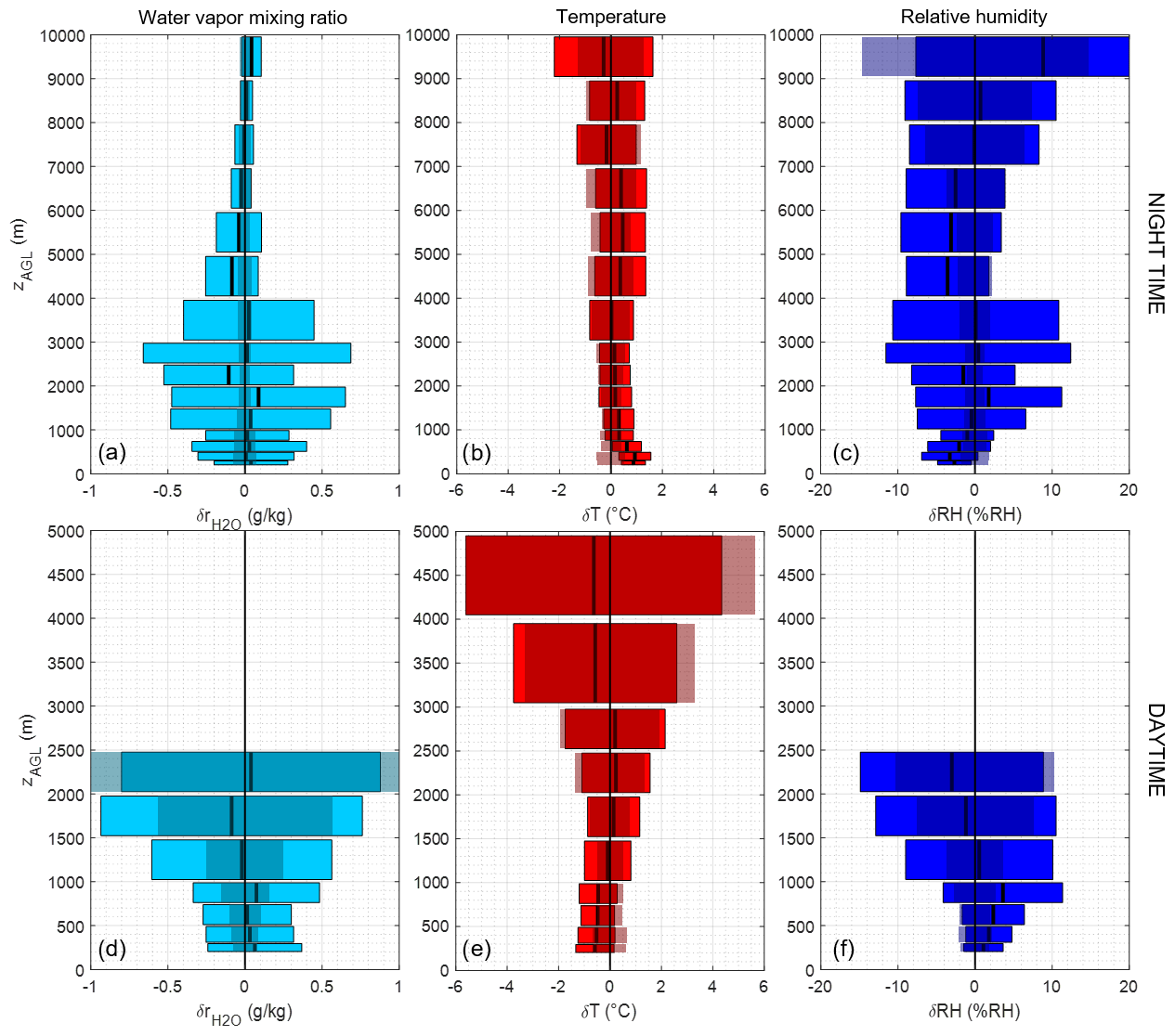
Figure 13 Residual deviations between lidar and Trappes radiosoundings in terms of WVMR, temperature, and relative humidity, for nighttime (a–c) and daytime (d–f), with mean deviation (thick lines) and RMSE (colored rectangles). The error corresponding to noise levels on the lidar signal is shown as darker rectangles. Cloudy profiles have been discarded. Daytime measurements are limited to SNRs above 5 for R (WVMR) and 20 for Q (temperature).

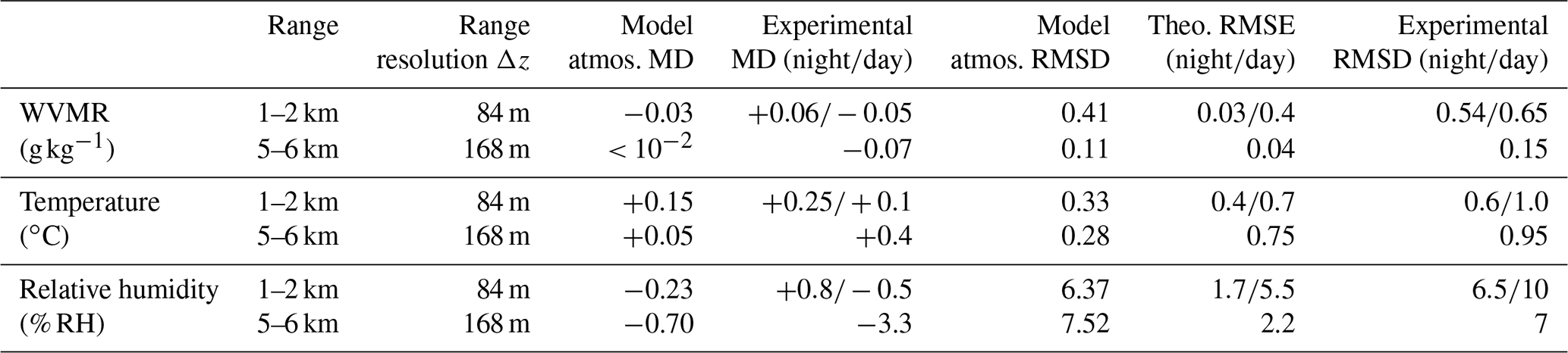
Table 4 Statistics of observed differences for $r_{{\mathrm{H}}_{\mathrm{2}}\mathrm{O}}$, T, and RH: experimental mean differences (MD), root-mean-square differences (RMSDs), averaged over two different range bins, in the low troposphere (1–2 km) and the free troposphere (5–6 km). Comparison to the “natural” atmospheric variability between the lidar and RS sites as modeled by the ECMWF/IFS ERA5 reanalyses (difference over the considered period between grid points nearest to each of the two sites) and to the theoretical root-mean-square error (RMSE) derived from the variance of the RR signals. The grid points are located 8 km WNW of the lidar and 2 km S of the RS launching station 18.3 km apart, and almost all RS trajectories below 6 km altitude are contained within the same “pixel” of the ERA5 fields as the RS station.

The reliability of this calibration along time has been tested by comparing to the same exercise performed 2 months later at the end of July 2020. After calibration in the same conditions as in May, we found K decreased by ∼7.3 %, and the temperature associated with a given value of Q^′ was ∼2.1 ^∘C higher. However, OR_R and OR_Q were still accurate within the reachable precision, i.e., ∼0.2 %. It was later proven that a malfunction of the laser seeder was responsible for a slow drift of the emitted wavelength. Thus, although a regular verification of the calibration is necessary, the measurement of the overlap ratios is reliable.

In Fig. 13, we examine the residual deviations between the lidar and the same series of radiosoundings used for the calibration. RH has been derived using Eq. (14) from lidar-estimated WVMR and temperature, and the pressure profile was given by radiosoundings. For each parameter $r_{{\mathrm{H}}_{\mathrm{2}}\mathrm{O}}$, T, and RH, we plot for daytime and nighttime profiles the mean and rms deviations averaged over wide range bins as colored bars as well as the propagated signal error as darker shaded areas. This allows us to compare the observed random error to what could be expected from the level of noise on the lidar measurements. Note that only profiles with good SNR unperturbed by clouds have been selected for this comparison.

On WVMR, the results show little bias, and rms deviation is dominated by spatial atmospheric variability at night and at low altitude (when SNR is high) and by lidar noise in all other cases. For temperature, most of the rms deviation is explained by noise; a significant +1 ^∘C bias is seen below 800 m during nighttime, opposed by a −0.5 ^∘C bias during daytime. This could be due to local effects in the diurnal cycle between LSCE and Trappes, although no such effect can be significantly highlighted in weather model reanalyses (described below). In Fig. 13c and f the consequences of this bias on relative humidity RH are plotted to be around 2 to 4 % RH, but the resulting error to be expected is also plotted. We see that with the defined averaging random error is around 2 % RH up to 5 $\mathrm{km}\mathrm{a}.\mathrm{g}.\mathrm{l}.$ during nighttime and 1 $\mathrm{km}\mathrm{a}.\mathrm{g}.\mathrm{l}.$ during daytime, growing fast above this level.

To support the above interpretation, in Table 4 we compare the experimental mean difference and rms difference plotted in Fig. 13, averaged over two altitude ranges (low troposphere (LT) at 1 to 2 km and free troposphere (FT) at 5 to 6 km), to (i) the natural variability of the atmosphere between the radiosondes at Trappes and the lidar at LSCE, as modeled by ERA5 reanalyses of the ECMWF/IFS weather model, and (ii) the expected random error given the noise level on the RR signals. Nighttime and daytime values are indicated in the LT, and only nighttime values are in the FT.

We see that the experimentally observed values of RMSD are rather consistent with the quadratic sum of the rms variability of the atmospheric variables between Trappes and LSCE and of the noise-induced RMSE. The excess random difference is thus well explained by the distance.

There is still a discrepancy with the mean difference of temperature below 1000 m between daytime and nighttime, however, probably due to the distance to the sounding station. Also, the model used to approximate a regularized correction is still imperfect at such short ranges and introduces small errors when the necessary correction is large and fast-varying. We aim to improve this in the future by launching radiosondes directly from the lidar site for calibration and by a better estimation the overlap ratios horizontally, for instance using a large folding mirror instead of tilting the lidar, which induces varying mechanical constraints on the optics.

5 Conclusions

During the qualification of the rotational Raman channels for the WALI lidar of LSCE, with the aim of providing profiles of relative humidity, we encountered important sources of bias that are seldom described in the now abundant literature involving such systems. We highlighted the predominant effects of the dependency of filter transmittance and detector sensitivity upon angle of incidence and point of impact, respectively. Because the latter parameters are directly proportional to field angle, they cause range-dependent biases on the RR–VR signal ratios that are several times greater than the required accuracy of lidars for temperature measurements (only 0.79 % for 1 ^∘C here), but less so for water vapor measurements. We established that this effect cannot be suppressed by using fiber optics between the receiver and polychromator, because scrambling of the lidar field of view does not happen radially in the fiber. Mitigation efforts impose the careful alignment of each filter at normal incidence to the input beam and the verification of the spectral transmittance of each channel on a spectrometer. The thermal stability of the polychromator is also of prime importance. Other significant bias sources include electro-magnetic perturbations of signal baselines and PMT gain variation, which must be mitigated. The impacts of fiber optics fluorescence and the measured laser line width or short-term wavelength drift were shown to be negligible in the WALI system.

After a measurement of RR–VR channel ratios during horizontal shots, which showed the significant impact of the above phenomena (up to 5 % bias on ratios below 300 m, ∼1 % higher), we calibrated and de-biased the WALI measurements using radiosondes launched from the nearby Trappes station of Météo-France. Between the de-clouded lidar measurements and the radiosonde profiles, the remaining mean differences are small (below 0.1 g kg⁻¹ on water vapor, 1 ^∘C on temperature), and rms differences are consistent with the expected error from lidar noise, calibration uncertainty, and horizontal inhomogeneities of the fields between the lidar and radiosondes. For relative humidity we thus reach a goal of ∼10 % RH random error and 5 % RH systematic error up to 9 km by night and 1.5 km by day, with 40 min time integration and progressive vertical integration of 15 to 360 m at 10 km. The systematic error on RH is dominated by bias on temperature, whereas the random error is dominated by noise on water vapor measurements.

Thus exhaustively qualified, the WALI system may be applied in the near future to exercises assimilating thermodynamic profiles in weather models, as is expected within the WaLiNeAs (Water vapor Lidar Network Assimilation experiment) project (Flamant et al., 2021). The long-term temporal evolution of Raman channel calibration, expected from various effects like differential PMT aging or laser seeder drift, induces biases variable in time over the timescale of such a project (several months). This aspect is becoming a main focus as the community works towards operational uses of weather Raman lidars (e.g., Hicks-Jalali et al., 2020).