the Creative Commons Attribution 4.0 License.
the Creative Commons Attribution 4.0 License.
 | 08 Dec 2021
Compositional data analysis (CoDA) as a tool to evaluate a new low-cost settling-based PM10 sampling head in a desert dust source region
Yangjunjie Xu-Yang
Fabrice Monna
Jean-Louis Rajot
Mohamed Labiadh
Gilles Bergametti
Béatrice Marticorena
This paper presents a new sampling head design and the method used to evaluate it. The elemental composition of aerosols collected by two different sampling devices in a semi-arid region of Tunisia is compared by means of compositional perturbation vectors and biplots. This set of underused mathematical tools belongs to a family of statistics created specifically to deal with compositional data. The two sampling devices operate at a flow rate in the range of 1 m3 h−1, with a cut-off diameter of 10 µm. The first device is a low-cost laboratory-made system, where the largest particles are removed by gravitational settling in a vertical tube. This new system will be compared to the second device, a brand-new standard commercial PM10 sampling head, where size segregation is achieved by particle impaction on a metal surface. A total of 44 elements (including rare earth elements, REEs, together with Al, As, Ba, Be, Ca, Cd, Co, Cr, Cu, Fe, K, Li, Mg, Mn, Mo, Na, Ni, P, Pb, Rb, S, Sc, Se, Sr, Ti, Tl, U, V, Zn, and Zr) were analysed in 16 paired samples, collected during a 2-week field campaign in Tunisian dry lands, close to source areas, with high levels of large particles. The contrasting meteorological conditions encountered during the field campaign allowed a broad range of aerosol compositions to be collected, with very different aerosol mass concentrations. The compositional data analysis (CoDA) tools show that no compositional differences were observed between samples collected simultaneously by the two devices. The mass concentration of the particles collected was estimated through chemical analysis. Results for the two sampling devices were very similar to those obtained from an online aerosol weighing system, TEOM (tapered element oscillating microbalance), installed next to them. These results suggest that the commercial PM10 impactor head can therefore be replaced by the decanter, without any measurable bias, for the determination of chemical composition and for further assessment of PM10 concentrations in source regions.
Please read the corrigendum first before continuing.
-
Notice on corrigendum
The requested paper has a corresponding corrigendum published. Please read the corrigendum first before downloading the article.
-
Article
(2953 KB)
-
The requested paper has a corresponding corrigendum published. Please read the corrigendum first before downloading the article.
- Article
(2953 KB) - Full-text XML
- Corrigendum
- BibTeX
- EndNote


At a global scale, mineral dust or mineral aerosols could represent about 40 % of the total amount of particles injected into the atmosphere each year (Boucher et al., 2013; Huneeus et al., 2011). Studying atmospheric mineral dust, which modifies atmospheric radiation and alters cloud properties, thus impacting climate, is essential to better understand the evolution of Earth's climate system (e.g. Mahowald et al., 2011). Mineral dust is also an important source of nutrients necessary for phytoplankton growth in the open ocean (e.g. Okin et al., 2011) and for terrestrial plant development (e.g. Okin et al., 2004). Most of the mineral dust present in the atmosphere comes from West Africa (Prospero and Nees, 1986; N'Tchayi Mbourou et al., 1997), with the Sahara as the main source (e.g. Ginoux et al., 2004). Accurate measurement of the chemical composition of aerosols is necessary for source tracing in aeolian studies (e.g. Scheuvens et al., 2013), which require aerosol data to assess global land degradation and climate change (e.g. Chappell et al., 2018).
In source regions of dry erodible material, high local wind speeds can move the largest and heaviest coarse soil particles (between 50 and 200 µm in diameter) on the soil surface, while the smaller particles (less than 70 µm in diameter) move by saltation, a jumping movement near the soil surface. Collisions between these particles and aggregates of the finest particles present at the soil surface release a large spectrum of smaller particles into the air (Marticorena and Bergametti, 1995; Marticorena et al., 1997; Alfaro and Gomes, 2001). These fine particles, particularly those smaller than 10 µm in diameter (PM10), can be transported by wind at higher altitudes over long distances (Gillette, 1981; Gomes et al., 1990; Shao et al., 1993; Shao, 2008). These particles are also a key parameter in air quality control (Kuklinska et al., 2015).
Efforts are made in atmospheric sciences to develop devices able to prevent unwanted collection of the largest particles with a 10 µm cut-off diameter. Commercially available standard sampling devices are commonly used to collect fine particles. One of the most popular is the PM10 sampling head, where size segregation is obtained by removal of the largest particles through impaction on an aluminium alloy plate. This process may however contaminate aerosol samples with metal particles because of friction between coarse particles and the metallic parts of the system. This is not an issue for simple aerosol mass determination but could generate problems if the objective is to define the chemical composition of airborne particles. It is well known that PM10 impactor inlet systems must be cleaned regularly: deposited particles that do not stick well on the impaction surface can bounce or can be de-agglomerated and re-entrained downstream, leading to oversampling (Le et al., 2019; Faulkner et al., 2014). Among other aerosol sampling head systems is the cyclone sampling device, where particles are separated by centrifugal force. Cyclone walls may be made of glass instead of metal, thus reducing potential secondary emission effects. This system is nevertheless difficult to manage because of its sensitivity to air pump flow rate (Haig et al., 2016). Impinger systems present a liquid impaction surface (Yu et al., 2016) and are well adapted for bio-aerosols but not for mineral particles. In this study, the potential of a new PM10 sampling head is evaluated in terms of mass collection efficiency and chemical composition accuracy. This new inlet uses the decantation principle; it can be built at low cost, using local materials because of its simple design and the broad availability of its components. Particle separation in this 125 mm diameter vertical tube decanter (VTD) system is based on gravitational settling counteracted by upward airflow. This system prevents collision between airborne particles and aerosol collector surfaces, so that sample contamination by metallic surface abrasion is minimized.
Source regions are good places to test possible biases introduced by the sampling head device in fine aerosol sampling because coarse aerosols larger than 10 µm are often present. Differences in cut-off diameter tuning will lead to differences in aerosol sample mass and chemical composition, as different amounts of the coarse particles present in the source zone will be collected. It is for this reason that we decided to compare the performance of two different sampling heads in a dry region of Tunisia. Aerosol chemical composition, including rare earth elements (REEs), and mass concentration of aerosols were measured at the same time using two sampling devices: a newly designed stainless steel decanter, VTD, and a brand-new aluminium alloy commercial PM10 sampling head (hereafter PM10), both operating at a flow rate of about 1 m3 h−1. The chosen sampling station is part of the International Network to study Deposition and Atmospheric composition in AFrica (INDAAF) and is equipped with a reference instrument for mass concentration measurements, a PM10 automatic weighing device (tapered element oscillating microbalance, TEOM). Masses deduced from elemental analysis of samples collected by each device were compared with one another and also with this third system, operating within the same flow rate range. The objective of this paper is to show that a low-cost decanter tube can replace an impaction-based PM10 sampling head for proper aerosol sampling. To achieve this objective, we use compositional data analysis (CoDA), an innovative tool for geochemical data analyses.
2.1 Aerosol sampling and direct measurements
A total of 16 paired samples were collected during a 2-week field experiment, at the Institut des Régions Arides campus, 20 km north of the city of Medenine, Tunisia. The collection site (33∘29′′58.62′′ N–10∘38′35.2′′ E), surrounded by dry lands, is 5 km south-west of the Boughrara Gulf. The two sampling devices were fixed to the roof of the highest building on campus, about 20 Both the VTD and PM10 were attached to a tubular stand, with a distance of about 30 cm between them (Fig. 1), to facilitate comparison of results. Aerosol samples were collected continuously from 29 March 2016 to 7 April 2016 using polysulfone open-face 47 mm filter holders (Nalgene®) and mixed cellulose ester filters, with a pore size of 0.45 µm (Whatman®). The filters were changed twice a day for each device at the same time: around 08:30 and 19:30, except for the pair YX29/30, which was exposed for 24 h.
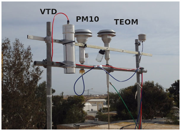
Figure 1From left to right, the VTD system, the PM10 sampling head, and the TEOM. Both the TEOM and PM10 heads are from the same brand: Tecora™ PM10.
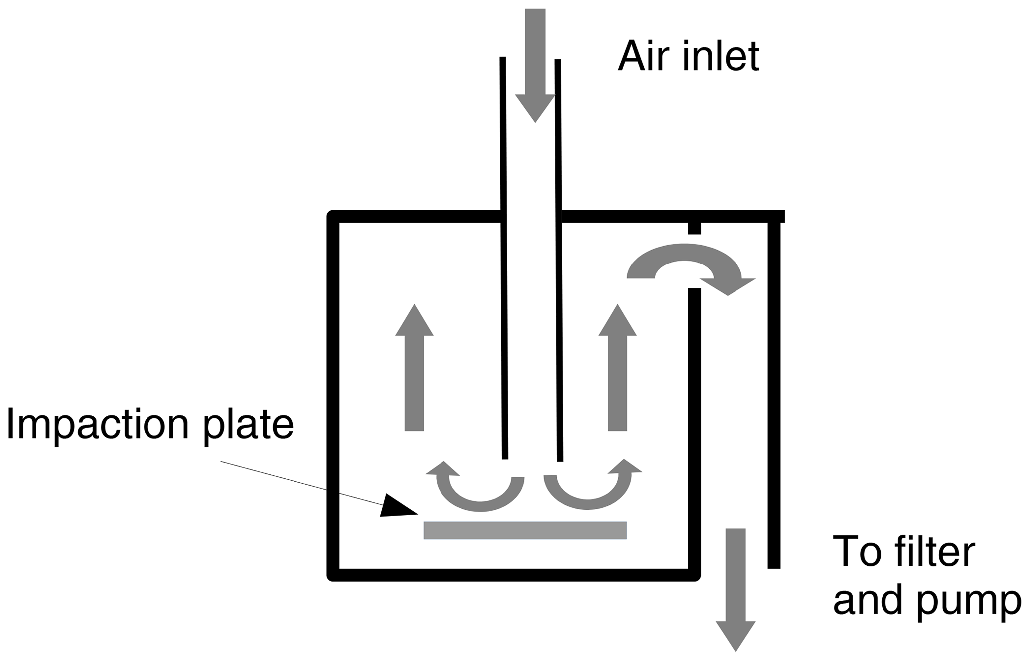
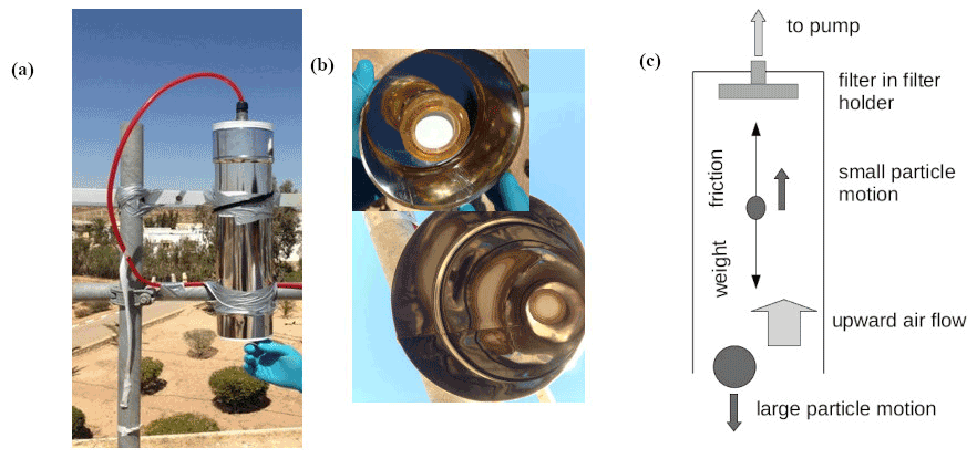
Figure 3The VTD system. (a) VTD installation on the roof of the building. (b) Two bottom-up views of filter on filter holder inside the decanter tube. (c) Diagram of decantation system.
Figure 2 shows the internal structure of the commercial PM10 sampling head (Tecora, Paris, France) installed, for the present study, with an aluminium alloy sampling plate. In the VTD system installed beside it (Fig. 3), air is pumped at the top of the tube and enters from the bottom of the tube. Fine particles are dragged upwards by the airflow and collected by the filter, but the largest particles do not reach the filter because of their weight. The terminal settling velocity for a particle of diameter D in a gravitational field is calculated using Stokes' law (e.g. Calvert, 1990):
where vg is the velocity of the particle when the steady state is reached; ρp is particle density; ρair is air density; g is gravitational acceleration; and μair is the dynamic viscosity of air.
When a particle is in the upward airflow, it is pulled up unless its gravitational settling velocity is greater than the airflow velocity, in which case it will settle down. A cut-off point occurs when gravitational velocity is equal to air velocity: only particles smaller than this cut-off size can reach the top of the VTD system and thus be collected on the filter. With a flow rate of 1 m3 h−1, the Reynolds number is equal to ≈ 50 inside the VTD. A laminar flow can be assumed and therefore a constant air velocity in the tube. The steady-state settling velocity of a particle is then reached when
where vair is the upward air velocity, Fair is the pumped air flux, and r is the radius of the cylindrical VTD system, which is about 6 times smaller than its height. The cut-off diameter (Dcut-off) can thus be rewritten as follows:
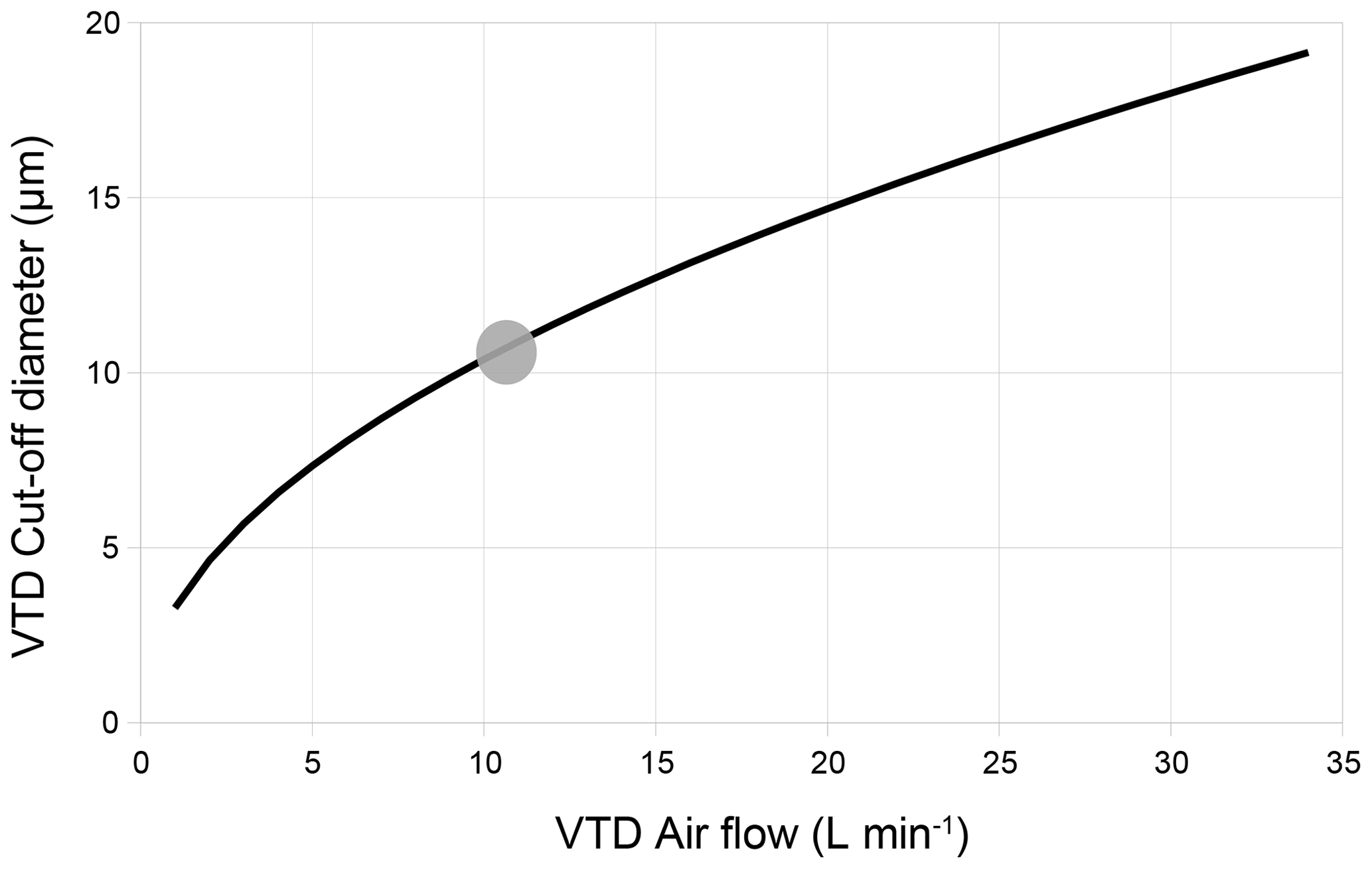
Figure 4Calculated particle cut-off diameter (µm) for the VTD as a function of airflow. Calculations are performed using Stokes' equations for a vertical cylinder with a diameter of 125 mm. The grey dot shows actual operating conditions, with measured airflows varying between 10 and 12 L min−1, leading to a cut-off diameter between 10 and 11 µm.
The Dcut-off value varies as a function of the pumped air flux when all the other parameters are fixed (Fig. 4), so that it can easily be tuned to 10 µm. In an ambient air loaded with particles including a significant amount larger than 10 µm, perfect systems should exclude these largest fractions and therefore collect the same aerosol mass concentration with the same composition.
A tapered element oscillating microbalance (TEOM, Thermo Scientific), equipped with the same commercial PM10 head, was also installed beside the VTD and the PM10 systems (Fig. 1). It measures the mass concentration of airborne particles directly, providing values considered as references for further comparison. A portable laser aerosol spectrometer (OPC, Model 1.108/1.109, Grimm), which measures particle size distribution over a large size range, was also installed ca. 3 m away from these three systems. A 1.111 radial symmetric sampling head (Grimm) was installed at the air inlet of the instrument to ensure reasonable capture efficiency for large particles. The OPC measures the number of particles within 15 diameter intervals between 16 diameter channels of 0.30, 0.40, 0.50, 0.65, 0.80, 1.0, 1.6, 2.0, 3.0, 4.0, 5.0, 7.5, 10, 15, 20, and 25 µm. Counting by OPC is converted into mass, assuming the lognormal distribution of spherical particles. The volume of Ni particles in the diameter interval is equal to , where is the geometric mean of di and di+1. With a particle density ρ, commonly chosen to equal 2.2 g cm−3, the PM10 mass, m10, is equal to the sum of all the channels under 10 µm:
while the mass of coarse particles larger than 10 µm is obtained by summing the channels over 10 µm. This coarse particle mass fraction should not be sampled by our sampling devices.
2.2 Washing procedure for sampling instruments
Prior to the field experiment, in the laboratory, 50 Petri dishes (PALL, filter storage box) were washed with detergent and rinsed with tap water, after which they were soaked in osmosed water containing 2 % of Decon90® for at least 15 h. They were then thoroughly rinsed with tap water followed by osmosed water before being soaked in acidified (HCl 1 %) osmosed water for 3 d. Finally, the Petri dishes were rinsed with Milli-Q® water (18 MΩ cm−1) and dried in an ISO-2 laminar flow hood. The filter holders and their PP boxes were cleaned using the same procedure. The PM10 head was disassembled, and each part was washed with tap water and detergent and then soaked in osmosed water containing Decon90® for several minutes. Finally, each part was washed with osmosed and Milli-Q water (18 MΩ cm−1) and dried in the laminar flow hood. The tube of the VTD was washed with detergent and rinsed with Milli-Q water before being dried in the laminar flow hood.
2.3 Sample digestion
The filters coated with dust samples were brought back to the laboratory (ISO-7 clean room) and dissolved in sealed Teflon® (PTFE) digestion vessels by 3 mL of a mixture of sub-boiled (9:1) for 18 h on a heater plate at 125 ∘C. All the Teflon vessels were previously cleaned with the detergent/acid procedure described above, completed with blank digestion. At the end of digestion, each vessel was opened, and the temperature of the heater plate was raised to 135 ∘C, until complete evaporation of all liquid. The temperature of the heater plate was then lowered to 80 ∘C, and 3 mL of a 30 % nitric acid solution was added to each vessel, which was then sealed. A period of 2 h later, the content of each vessel was transferred into a 60 mL polypropylene bottle (thoroughly detergent/acid cleaned), by adding Milli-Q water. Laboratory blanks (no filter), four field blanks (pristine filter), and two finely ground geostandards (SCO-1 and MAG-1 from USGS) were also prepared following the same digestion procedure.
2.4 Chemical analyses
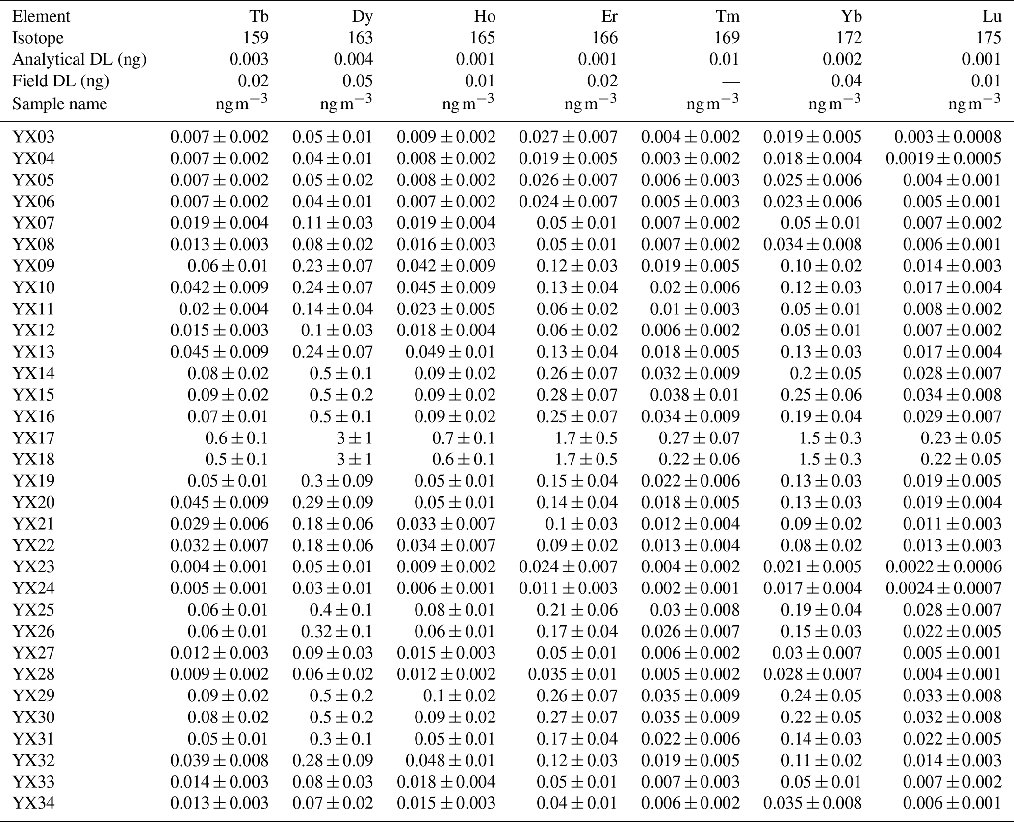
An ARCOS (Spectro-Ametek) ICP-AES, equipped with a CETAC ultrasonic nebulizer, was used for elemental determination of Al, Ba, Ca, Cr, Fe, K, Li, Mg, Mn, Na, P, Sc, S, Sr, Ti, Zn, and Zr. A field-sector high-resolution inductively coupled plasma mass spectrometer (FS-HR-ICP-MS), Thermo Element 2, equipped with a concentric micro-nebulizer in a cyclonic nebulization chamber, was used for elemental determination of As, Be, Cd, Co, Cu, Mo, Ni, Pb, Rb, Se, Tl, U, V, and REEs. External linear calibration was performed for all elements analysed with ICP-AES, by measuring a set of multi-elementary solutions with concentrations up to 250 µg L−1. The intercept was computed as the average of eight replicates of a blank sample (ultra-pure nitric acid diluted in Milli-Q water). High-resolution analysis avoids polyatomic interference for elements lighter than arsenic and also for REEs (Heimburger et al., 2013). The FS-HR-ICP-MS was externally calibrated for all elements analysed, with 14 replicates of a blank solution and 5 replicates of a 1 µg L−1 multi-elementary solution. The first analytical detection limit was obtained with analytical blanks and digestion with dilution water and acid reagents only, while the second field detection limit was obtained with blank filters transported to the field. For most of the elements, quantities found in blank filters were higher than analytical detection limits, so that blank correction used the average quantity found in blank filters. For a few elements (Pr, Eu, Tb, Dy, Ho, Tm, and Lu), blanks were below detection limits, so no blank correction was made. Seven elements (As, Cd, Cr, Mo, Ni, Sc, and Se) are not discussed because they cannot be handled by the statistical tools used here, as at least one measured value was below the field or analytical detection limit. Analytical results are provided in Appendix A, Tables A1–A7.
2.5 Validation of analytical methods
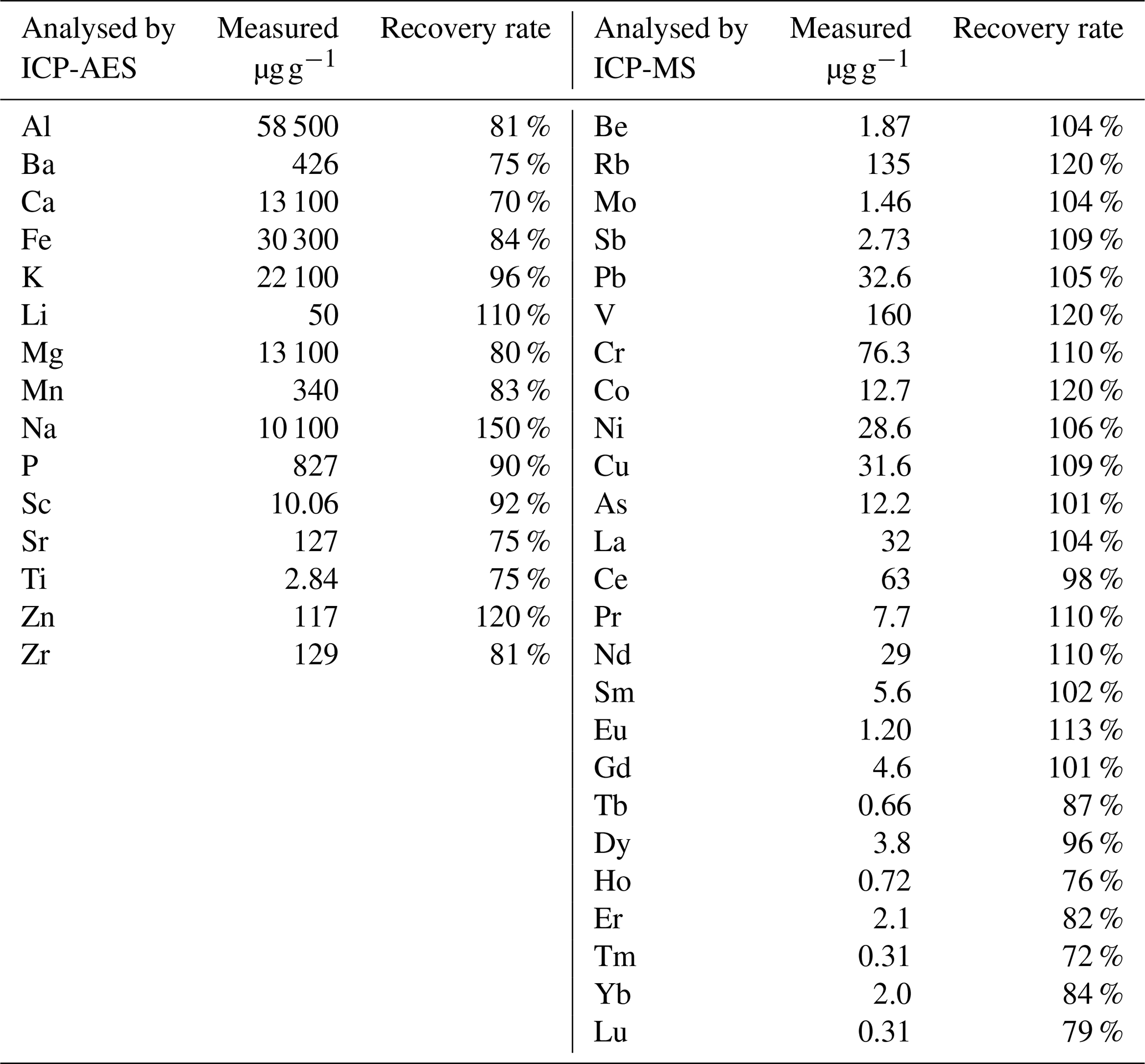
There is no commercially available certified reference material comparable to the fine aerosols collected on filters. Two geostandards were therefore used as proxies: SCO-1 (typical of Upper Cretaceous silty marine shale) and MAG-1 (a fine-grained grey-brown clayey mud with low carbonate content, from the Wilkinson Basin of the Gulf of Maine). They were hand-crushed for 30 min in an agate mortar to approximate aerosol grain size. The powders produced were deposited on a filter at the smallest amount that can be weighed (around 10 mg with an accuracy of 0.2 mg) to obtain a mass as close as possible to field aerosol samples. A table with individual recovery rates, as well as individual measurement results for each certified element and aerosol sample, is proposed in Appendix B, Table B2. Recovery rates for most elements ranged from 80 % to 120 % for SCO-1 and MAG-1 but could not be calculated for S, Se, and Tm because no value was available for comparison.
2.6 Computation of total aerosol mass concentration
The PM10 mass concentration was not directly measured because of the low expected weight and the nature of the cellulose-ester filters which are sensitive to moisture. That is why a TEOM was installed, as it directly provides aerosol mass concentration in air. In this region, almost all the particle mass can be assumed to be carried by silicate crustal particles, sea salts, sulfuric acid (H2SO4), and additional calcium in the form of calcium carbonate (CaCO3). A chemical reaction occurs between calcium carbonate and sulfuric acid, producing gypsum (CaSO4•2H2O) and preventing the simultaneous presence of sulfuric acid and calcium carbonate (Mori et al., 1998). If carbonate predominates over sulfuric acid, the total particle mass concentration is computed as
If sulfuric acid predominates over carbonate, then
where [crust particles]air is estimated using aluminium and a crustal composition model, where aluminium accounts for 7.1 % of the mass (Bowen, 1966). This value is consistent with that of 7.09 ± 0.79 % observed by Guieu et al. (2002) for Saharan dust.
[sea salt] is estimated using sea salt sodium and a seawater composition model (Dickson and Goyet, 1994), where sodium accounts for 30.9 % of sea salt mass. Sea salt sodium is deduced by subtracting crustal sodium from total sodium, crustal sodium being deduced from aluminium (Rahn, 1976), and a crustal composition model, where the ratio is equal to 0.0887 (Bowen, 1966):
where [CaSO4 • 2H2O], [CaCO3], and [H2SO4] are calculated using additional calcium and additional sulfur not included in crustal and sea salt estimation. Ca∗ and S∗ are defined respectively as calcium and sulfur of neither sea salt nor crustal origin. Ca∗ and S∗ are computed using the same crustal and sea salt composition models previously used:
Depending on the resulting products of calcium carbonate with sulfuric acid reaction, the mass associated with additional calcium and sulfur is computed as follows:
where MX is the molar mass of the compound or element X.
2.7 Multivariate analysis for compositional data (CoDA)
Compositional data are, by nature, difficult to handle straightforwardly. Any given component cannot vary independently from the others because the sum of all components is always equal to 100 %. If this closure constraint is not taken into account, spurious correlations and biased conclusions are to be expected (Van der Weijden, 2002). Appropriate mathematical tools must therefore be selected to overcome this drawback. These questions are extensively discussed in several papers (Aitchison, 1986, 1992, 2005; Barceló-Vidal et al., 2001; Filzmoser et al., 2009; Egozcue et al., 2003). Briefly, the suitable sample space of any compositional vector x, representing a D-part subset of a whole , is the simplex SD, as defined by Aitchison (1986). This technique is particularly well adapted to situations where elemental ratios are more relevant than absolute concentrations.
Let and denote two compositional vectors in SD. Then z, corresponding to the perturbation of x by y, in SD is given by
with C the closure-to-unity operation defined as
The neutral element of the perturbation is , and , while the perturbation vector expression compositional change from y to x, noted x⊖y, is equal to , with (von Eynatten et al., 2002; Aitchison and Ng, 2005). The centred log-ratio (clr) transformation is commonly performed to open the data before applying any multivariate techniques based on correlation:
where gm(x) denotes the geometric mean of the D parts: . A principal component analysis (PCA) can then be computed on transformed data to summarize the structure of the data in a lower dimensional space (ideally two for the sake of simplicity of projection on a plane). A compositional biplot, where both samples and variables are plotted in the same space, can be used as a user-friendly graphical representation, but it differs from the original biplot by Gabriel (1971) in the sense that rays formed by the variables are proportional to the standard deviation of their log ratios and that the length of a link between arrow heads of two rays represents the standard deviation of the log ratio between these compositional parts (Suárez et al., 2016). Practically, the “acomp” (closure operation) and “princomp” (PCA projection) functions used here were provided by the “compositions” package for the R software (R Core Team, 2014), which was specifically designed to analyse compositional data (van den Boogaart et al., 2014). This data processing based on log-ratio computing is named “compositional data analysis” (CoDA).
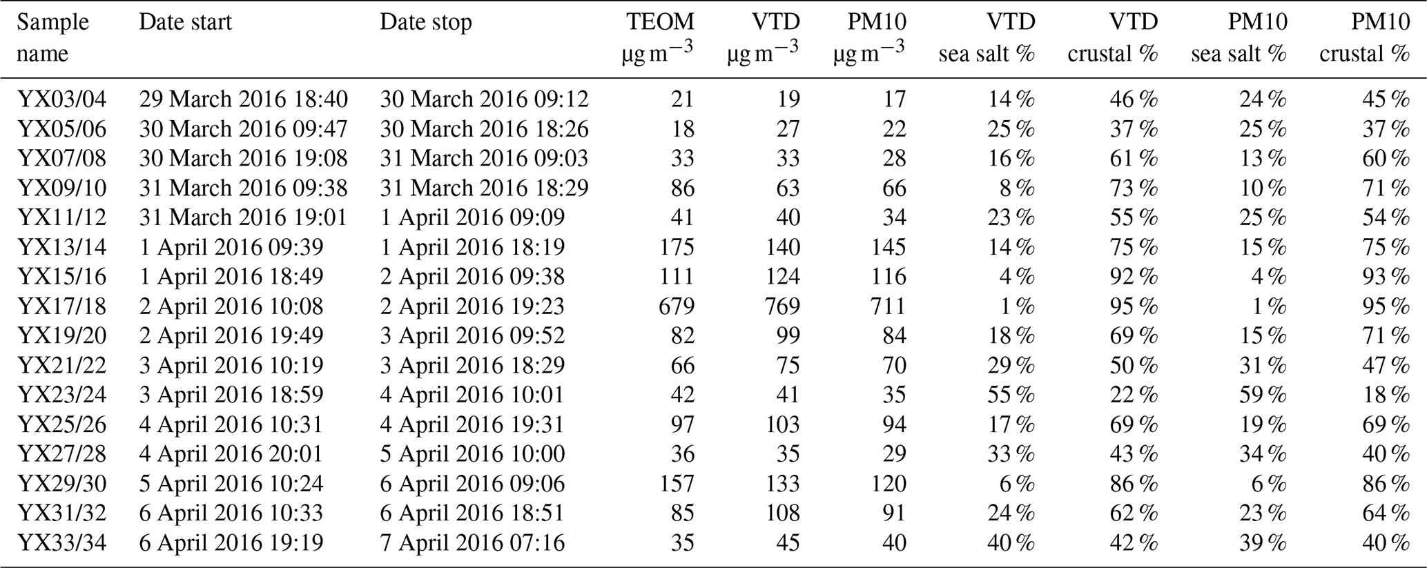
Table 1Sampling dates (local time) and aerosol mass concentrations directly measured by TEOM and calculated from chemical analysis of samples collected by the VTD and PM10, respectively. Masses derived from chemical analyses are computed using equations presented in Sect. 2.6. The last four columns (right) display mass proportion of sea salt and crustal aerosol for VTD and PM10 samples. Detailed results are shown in Tables E1 and E2 (Appendix E).
3.1 Variability of sampling conditions
The sampling site can be influenced by local and remote soil dust emission, by sea salt, and by anthropogenic emissions. During the sampling campaign, a broad variety of meteorological conditions were observed, allowing different aerosol sources to be sampled. Average local wind speed varied from about 1 to 7 m s−1, with no preferred direction (Appendix C, Fig. C1). Backward air trajectories are presented for each sample pair in Appendix C (Figs. C2–C5), indicating their differences in origin, leading to a variety of conditions for aerosol loading. Atmospheric aerosol loading presented a large range of values, from 21 to 679 µg m−3 (Table 1, TEOM values), with great variations between marine vs. crustal proportions in any given sample pair.

Figure 5Daily average particle mass concentration size distribution in air on 31 March (a, aerosol concentration ca. 40 µg m−3), 6 April (b, aerosol concentration ca. 100 µg m−3), and 2 April, morning (c, aerosol concentration ca. 700 µg m−3). Measured using the Grimm OPC.
3.2 Size distribution of the sampled aerosol
The fraction of particles larger than 10 µm suspended in the air is shown by OPC measurements. For the entire field experiment, this coarse fraction represents, on average, 34 % of the total mass concentration of aerosols as plotted in Fig. 5, for three given periods with various dust concentrations. The presence of a significant amount of large particles in air makes the systems sensitive to possible inaccuracy and variations in their cut-off diameters: if the cut-off diameter were not the same for each sampling head in a given sample pair, the amount of large particles collected would not be the same and would produce differences in sampled aerosol mass concentration. Because chemical composition may be dependent on particle size, differences in cut-off diameters would also produce differences in chemical composition.
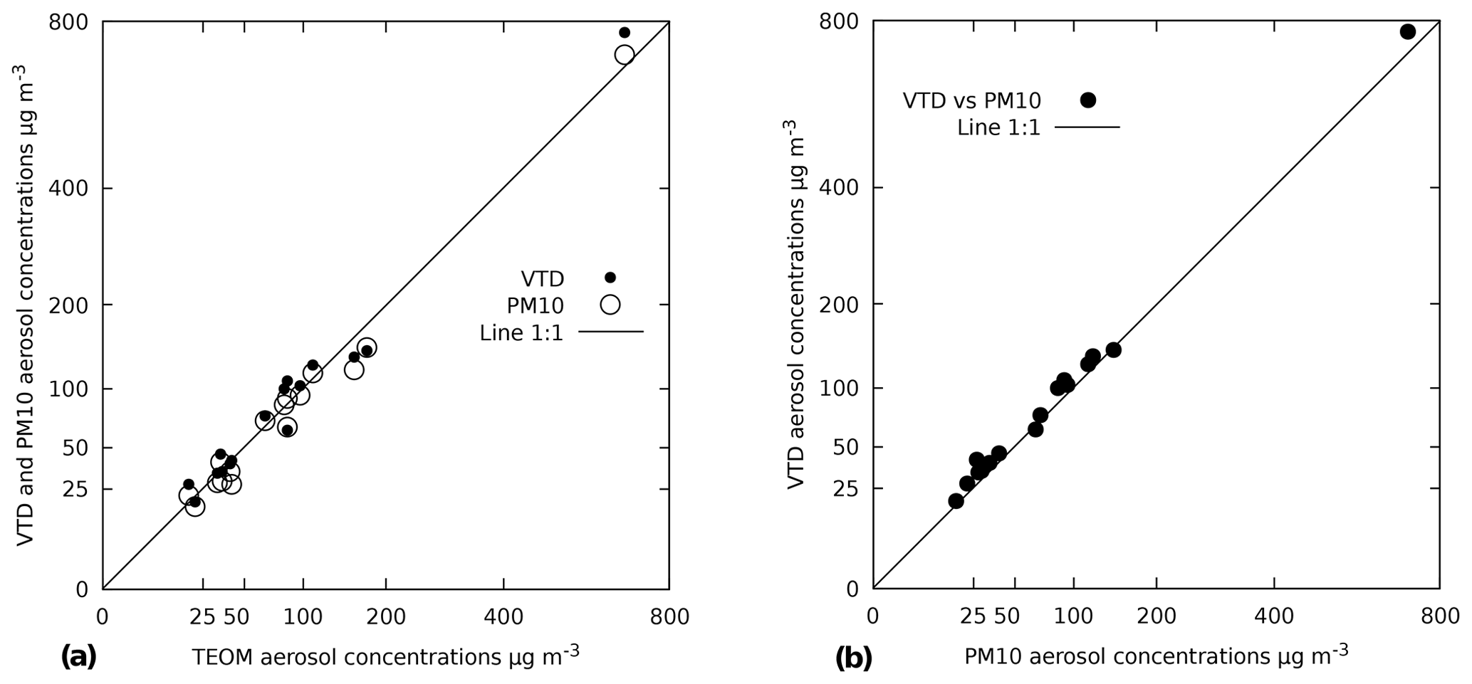
Figure 6Comparisons of sample masses using a square-root scale. The lines y=x are also shown. (a) Plot of chemically deduced mass of VTD and PM10 sampling heads vs. TEOM measurement. (b) Plot of chemically deduced mass of VTD vs. PM10 sampling heads.
3.3 Total aerosol mass concentration in air
Comparisons of the measured mass concentrations between the VTD, PM10, and the reference instrument TEOM are shown in Fig. 6 and Table 1. Mass concentrations are averaged during each collection period. Plotted concentrations vary from 21 to 680 µg m−3 within a range that can be cleverly plotted using a square-root scale (Verrall and Bell, 1969). Masses of particles collected by the VTD and PM10, deduced from calculations using Al, Na, S, and Ca, fit the TEOM values (Fig. 6a). Similar results are observed for each VTD and PM10 sample pair (Fig. 6b), suggesting the same collection efficiency for both sampling heads and hence the same cut-off diameter. The median value of the relative mass differences between the VTD and PM10 is +12 %, and values range from −3 % to +22 %. Such variability is of the same magnitude as that observed by Heal et al. (2000) or Hitzenberger et al. (2004) in PM10 and PM2.5 inter-comparison exercises or by Motallebi et al. (2003) in a comparison of entire monitoring networks. An orthogonal regression, also known as total least squares, was performed on the data presented here by treating the variances of x and y symmetrically. Orthogonal regressions were performed twice, with and without the highest point, which could potentially be considered an outlier. Regression slopes for the three possible combinations (PM10 vs. TEOM, VTD vs. TEOM, and VTD vs. PM10), with and without the highest point, are between 0.94 and 1.03. The value of 1 is always included in the 95 % confidence level interval associated with each slope, and intercepts are not significantly different from zero (see Tables D1 and D2 in Appendix D), suggesting that any potential bias is too small to be identified with our data. To summarize, the differences observed between aerosol masses measured by the three sampling systems are much lower than the daily variability observed during the field experiment. The coherence between direct measurement of masses (TEOM) and “chemical” weighing shows that substances not taken into account in our chemical budget (ammonium and organic molecules) do not significantly contribute to the total aerosol mass here.
3.4 Compositional data
The aim is now to compare chemical compositions of samples collected simultaneously by both the VTD and PM10, as differences may appear due to contamination or size segregation of particles. Note that major and trace elements are treated separately from the REEs in the following because of the particular importance of REEs as tracers of mineral particle origin (Wang et al., 2017).
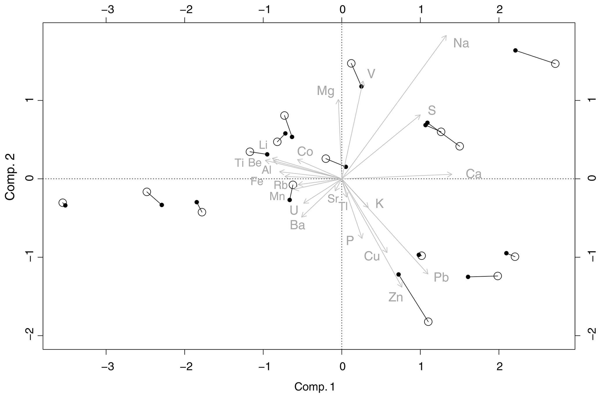
Figure 7Biplot for the two sampling devices (all elements except REEs). PM10 samples are figured with circles, and solid discs represent VTD samples. Lines between PM10 and VTD symbols link paired samples. Percentages of variability explained by the first two components are 61 % and 16 %, a total of 77 %.
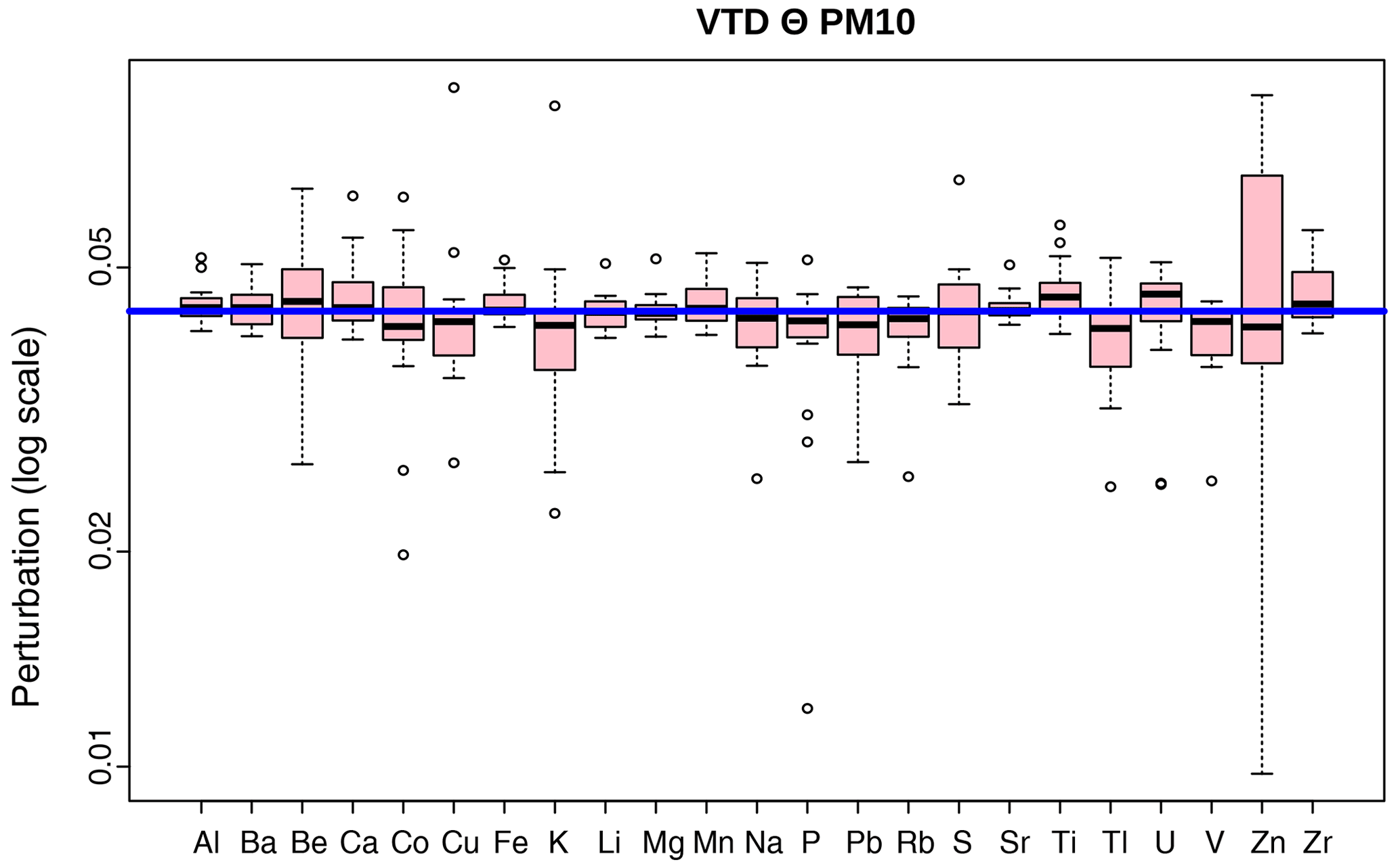
Figure 8Perturbation diagram as box plots for paired samples (all elements except REEs), measured by PM10 and the VTD. The horizontal blue line represents no perturbation.
3.4.1 Major and trace elements
The first two axes of the compositional biplot built from major and trace elements, without REEs, explain 77 % of the total variance (61 % and 16 %, respectively), a high value, considering that 23 variables are taken into account for the analysis (Fig. 7). The variability between each pair of samples (i.e. collections by PM10 and the VTD on the same day), figured by the segment linking the two samples of the same pair, appears to be much lower than the variability observed within the entire set of samples. In other words, each dust event can be characterized properly with respect to the others, independently of the sampling device used. This finding is in good agreement with a close examination of compositional changes between PM10 and the VTD for each pair of samples, expressed as perturbation vectors: VTD⊖PM10, with (Fig. 8). Interestingly, the neutral element , which indicates no perturbation, is included inside all the box plot quartiles. No systematic compositional shift, in terms of elemental ratios, can therefore be observed between the two sampling heads, at least for these elements, and it can be concluded that sample composition is not affected by the type of sampling head. Note, however, that Zn exhibits the greatest variability, suggesting noticeable random contamination. The slight differences observed between the two sampling heads in each paired sample are found to be correlated neither to air aerosol concentrations nor to wind speed. Potential contamination issues due to aluminium impaction plates were among the main reasons why sampling heads were tested in the field with natural aerosols. No systematic compositional differences were observed between the two sampling heads although they are made of different alloys. This observation strongly suggests that neither of the two devices (brand-new PM10 and VTD) would contaminate natural samples collected during this campaign.
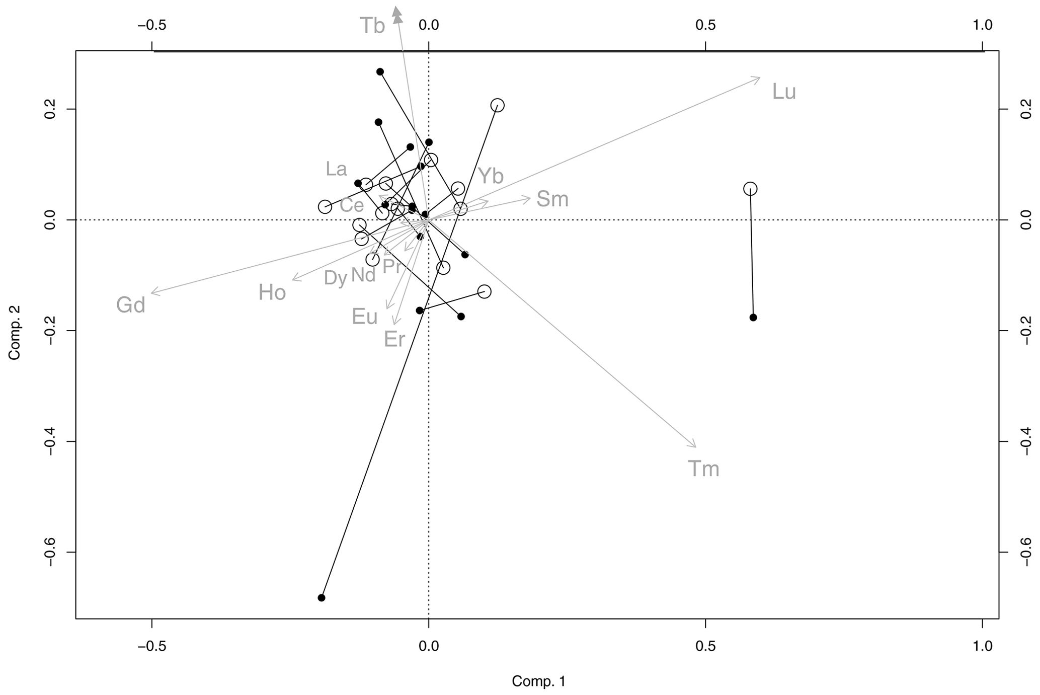
Figure 9REE biplot for the two sampling devices. PM10 samples are figured with circles, and solid discs represent VTD samples. Lines between circles and discs link paired samples. Percentages of variability explained by the first two components are 29 % and 22 %, a total of 51 %.
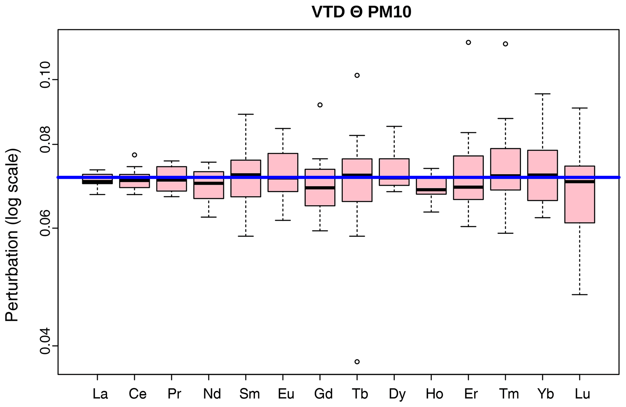
Figure 10REE perturbation diagram as box plots for paired samples, measured by PM10 and the VTD. The horizontal blue line represents no perturbation.
3.4.2 Rare earth elements (REEs)
In the compositional biplot built from REEs, only 51 % of the total variance is explained by the first two axes (Fig. 9). This value is much lower than that obtained above for the other chemical elements (77 %) but with only half the number of variables. The corresponding perturbation vector diagram again shows no systematic difference between the two sampling heads (Fig. 10). Because REEs essentially come from a stable crustal source, log ratios between these elements vary little within the sample set (almost 10 times less than the variability observed for the other elements). This stability explains why the percentage of variance expressed by the first two principal components is so low.
To test whether the differences observed between the two systems might be explained solely by analytical error, the behaviour of identical duplicate samples was simulated: 16 new pairs of compositions were generated, by pairing each VTD sample with a modified sample, where each REE measurement was randomly shifted inside the given uncertainty interval of that REE. These new pairs of simulated samples were then represented as a biplot (Fig. F1, Appendix F), producing results very similar to those observed for the real (VTD and PM10) paired samples. During this field campaign, the REE profiles were found to be stable and unaffected by the design of the sampling head.
The main advantage of this new PM10 inlet is its simple design associated with its low cost and the broad availability of the components, making this new inlet easy to build locally by everyone. A second possible reason to use the VTD is easier maintenance. Compositional data analysis tools have been used to present large sets of measurements at a glance, allowing us to perceive the compositional similarity of paired samples quickly and directly. No significant differences between the laboratory-made decanter sampling head and the commercial PM10 sampling head (based on impaction) were observed in terms of aerosol composition (including REEs) and total mass concentration, for samples collected in a source region of mineral dust, under very different meteorological conditions. In the source region investigated, where particle mass concentrations ranged from 20 to 700 µg m−3 according to TEOM values, the chemical composition of the PM10 aerosol fraction was therefore unaffected by the sampling head design. Consequently, both devices can be used for the determination of mass and chemical composition of aerosols in source regions or even simply to determine mass by gravimetry. An aerosol survey network can therefore be built using a combination of the two sampling devices without any measurable consequences for data reliability or consistency. This would also be the case for a time series if a PM10 was replaced by a VTD or vice versa.
Raw data of the paper are presented in Tables A1–A3 for ICP-AES measurements, in Tables A4 and A5 for ICP-MS measurements, and in Tables A6 and A7 for REEs measured with ICP-MS. “DL” is “detection limit”, expressed in mass on the filter. “<” is “less than concentration detection limit”; this concentration detection limit must be calculated by dividing the DL value (expressed in mass) by the air volume. Uncertainties are given for a 95 % confidence interval. The air volume uncertainty is constant at 1 % and not displayed.
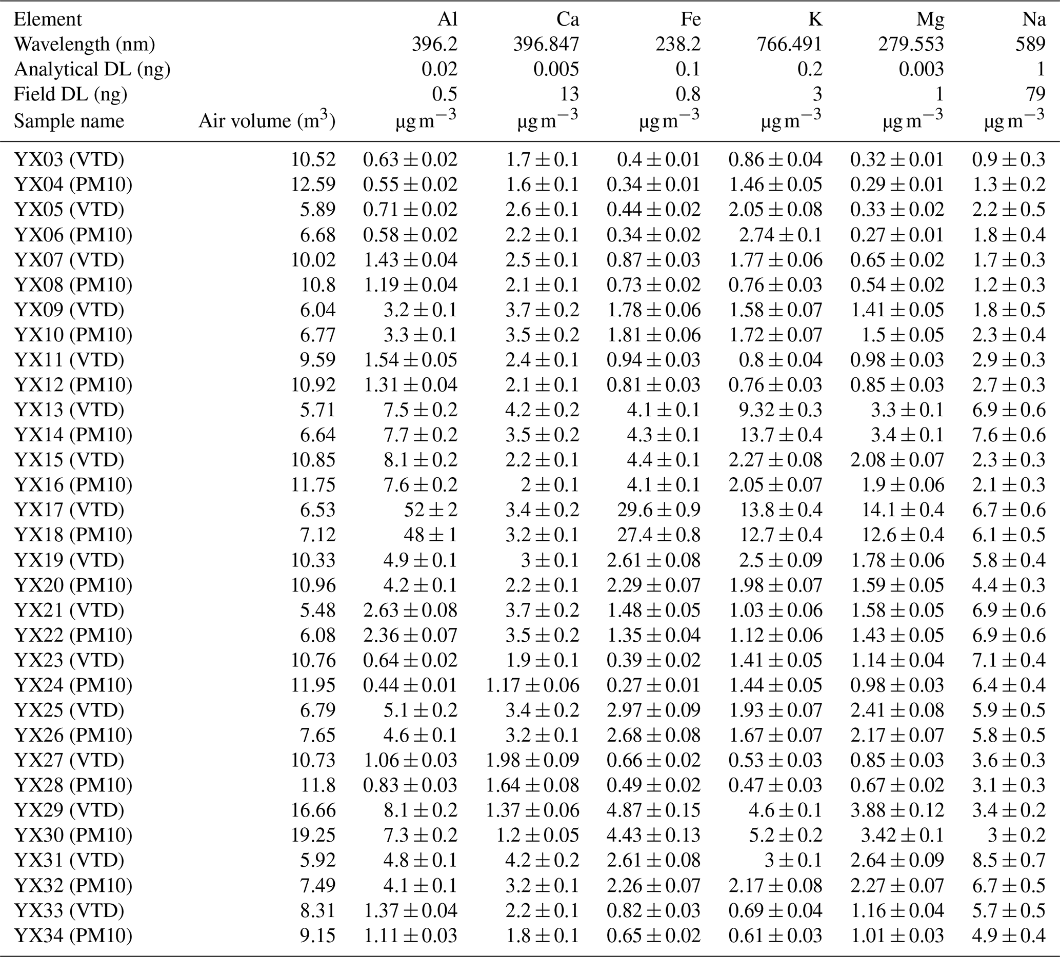
Table A2Elemental air concentrations measured with ICP-AES, continued.
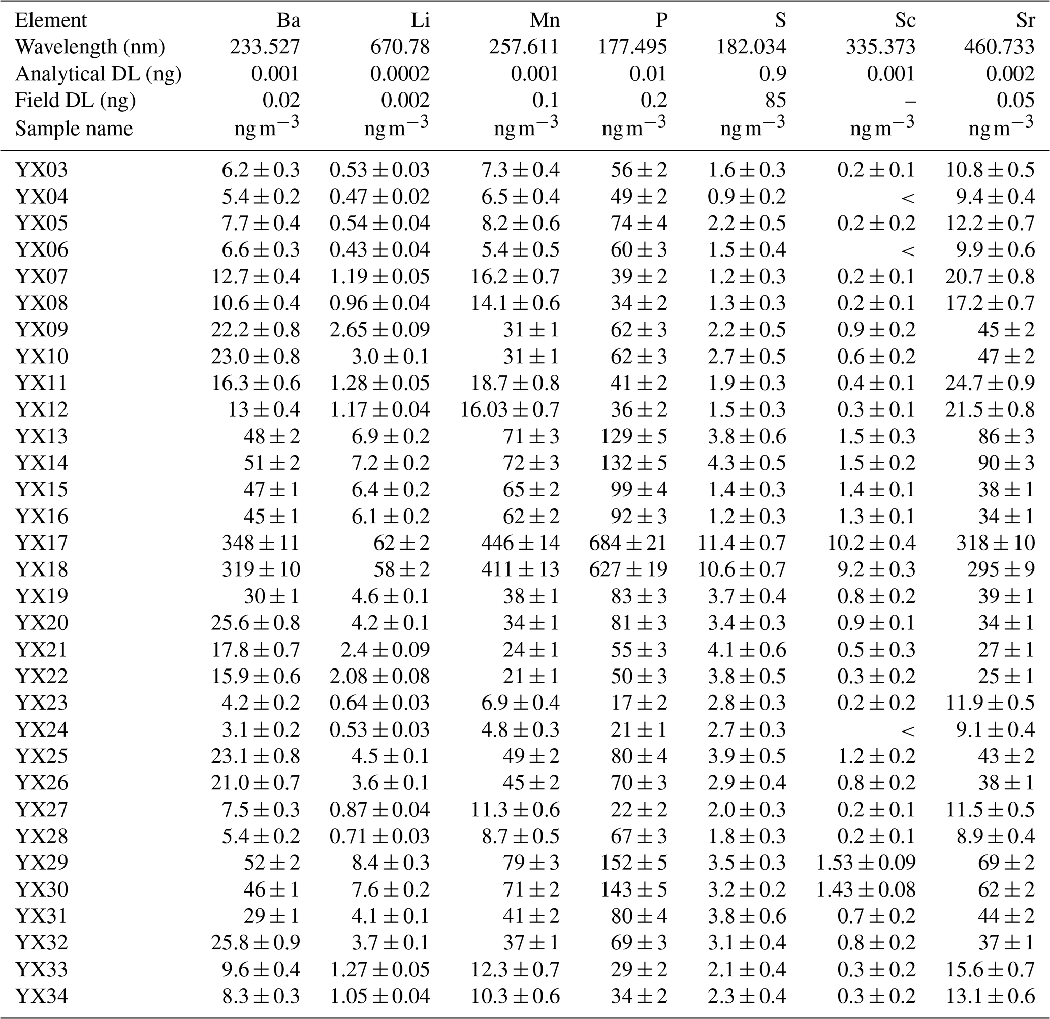
Table A3Elemental air concentrations measured with ICP-AES, continued.

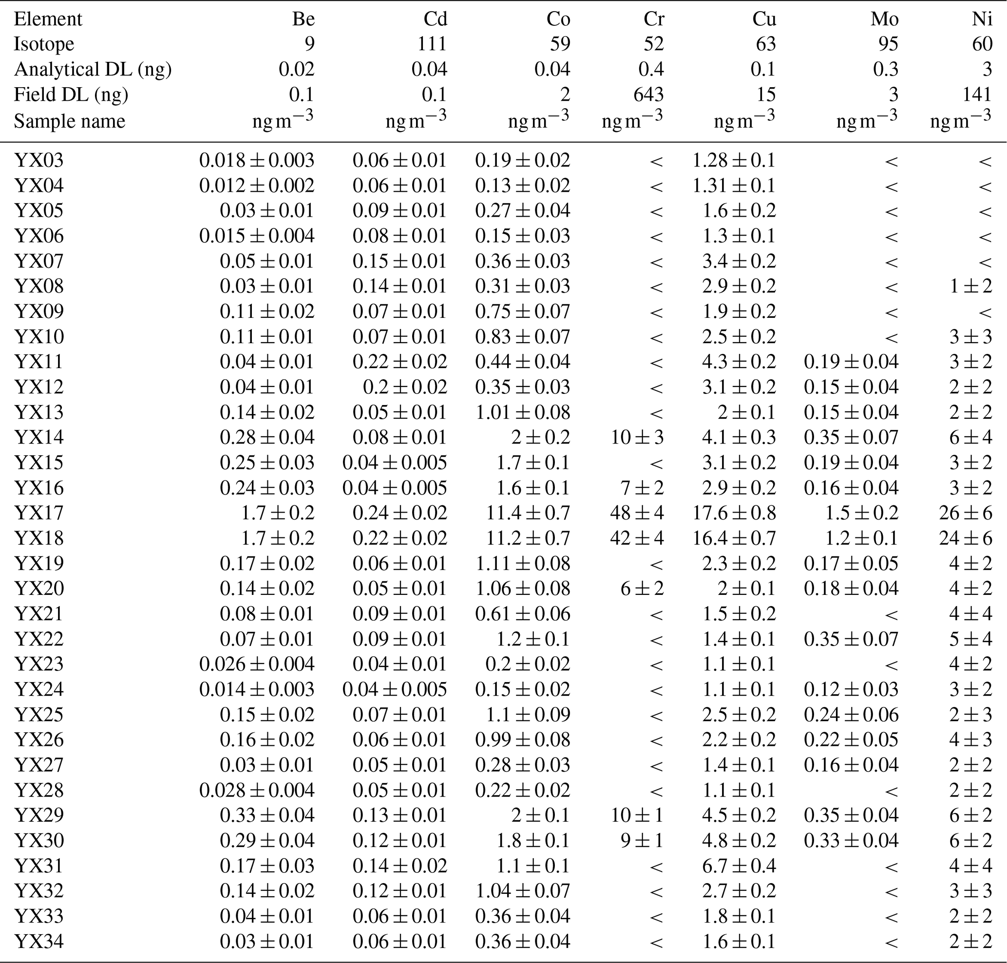
Table A5Elemental air concentrations measured with ICP-MS, continued.

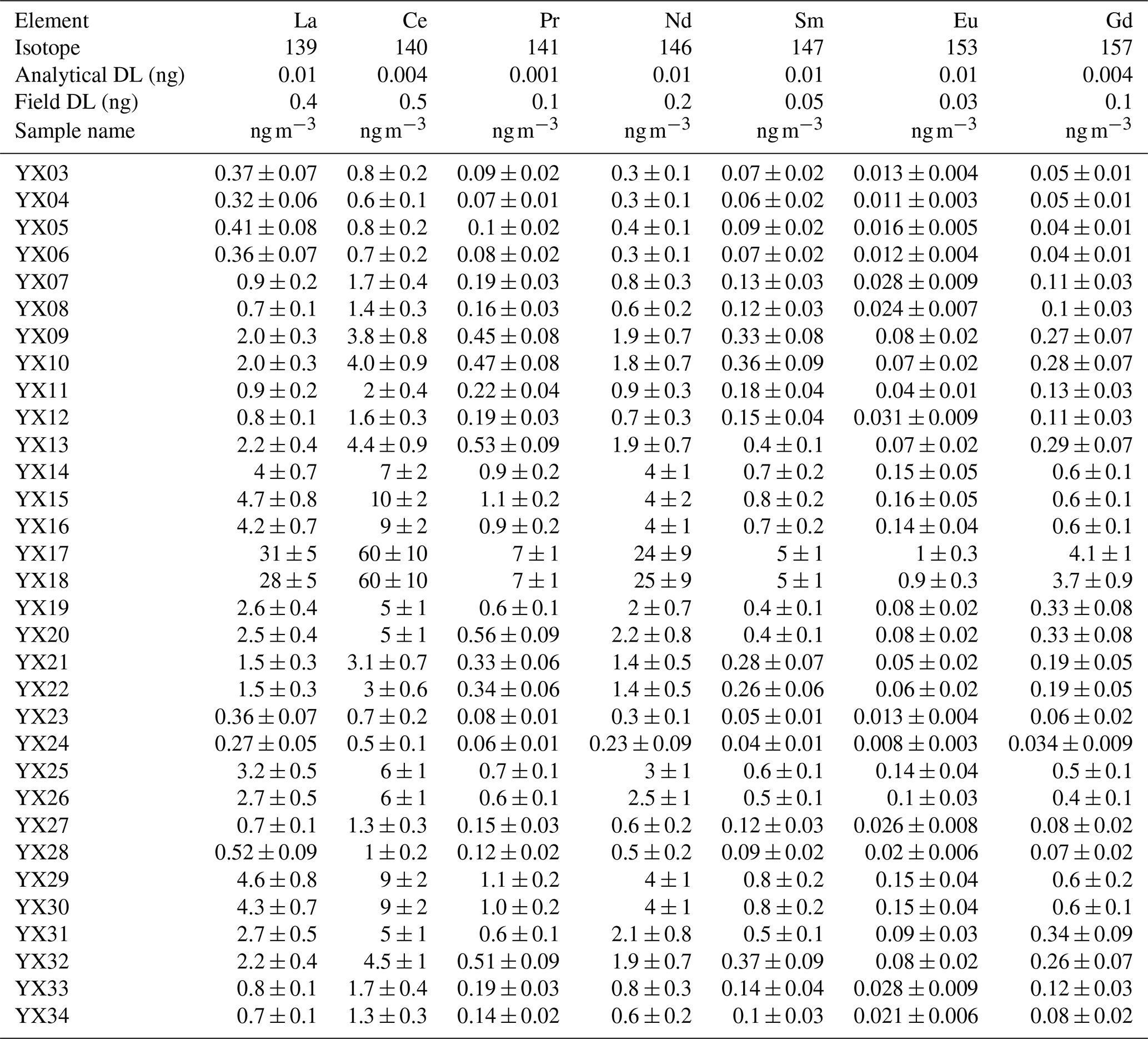
Table A7REE air concentrations measured with ICP-MS, continued.
Recoveries of geostandards MAG-1 in Table B1 and SCO-1 in Table B2.
Table B1MAG-1 recovery rates. Elements have a recovery rate between 68 % and 130 %, except for Zn and Ni. The very low amount of geostandard used (< 10 mg) could explain the difference observed in recovery rates because subsampling heterogeneity is possible with such small amounts. Zn and Ni are overestimated, probably due to contamination.
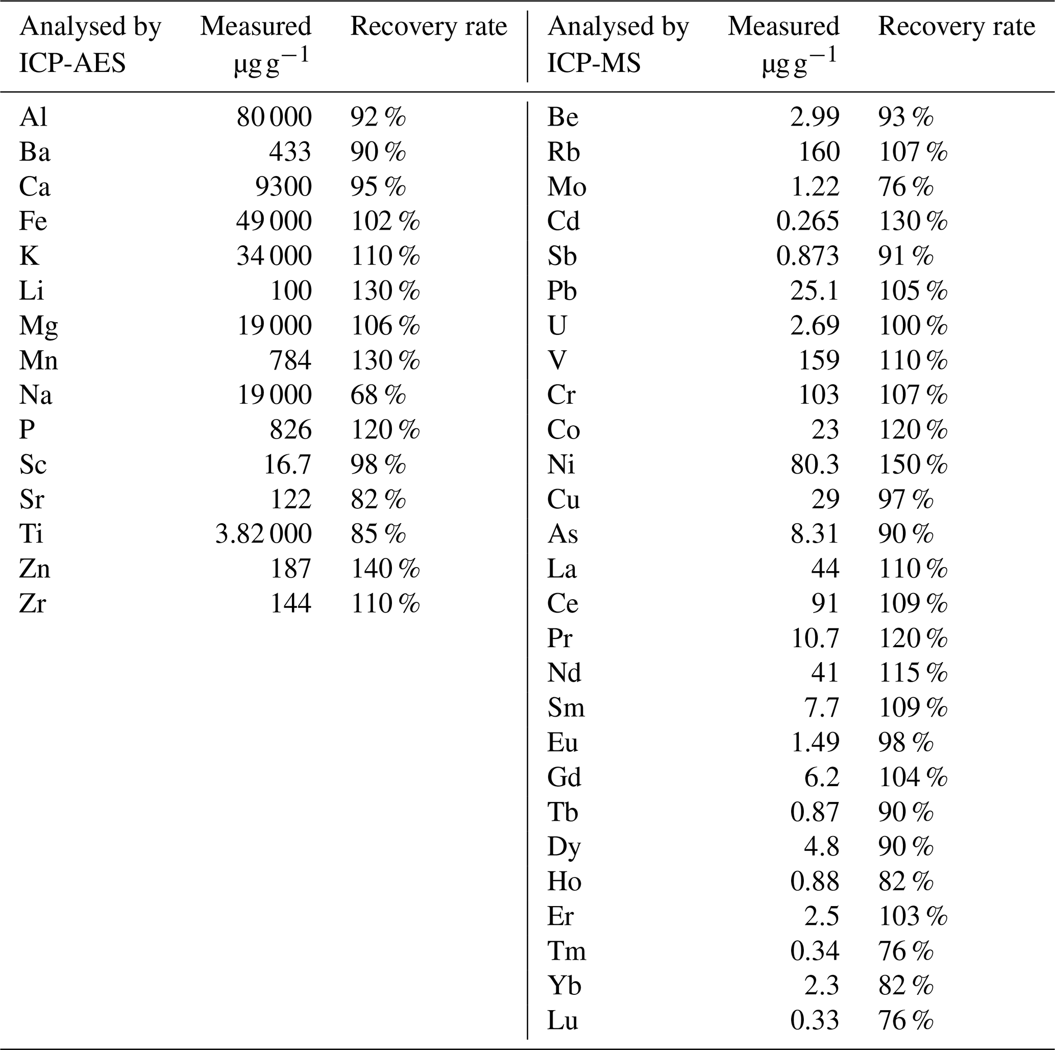
Table B2SCO-1 recovery rates. Elements, except Na (recovery rate = 150 %), have a recovery rate between 70 % and 130 %. The very low amount of geostandard used (< 10 mg) could explain the difference observed in recovery rates because subsampling heterogeneity is possible with such small amounts.
Wind speed and direction are measured continuously at the sampling location, and backward air trajectories are calculated using the online facility on NOAA HYSPLIT model web pages (Stein et al., 2015; Rolph et al., 2017). Trajectories for a 24 h period are calculated every 6 h (at 00:00, 06:00, 12:00, and 18:00).
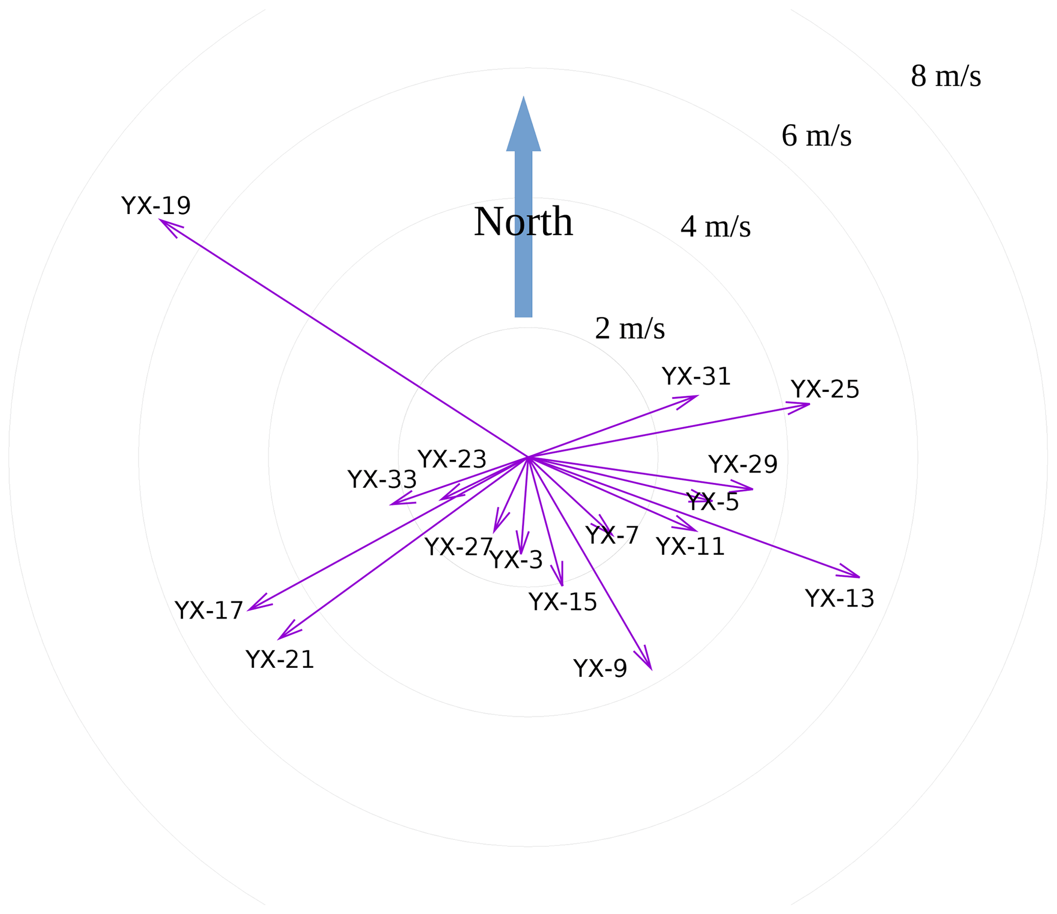
Figure C1Vector representing local wind conditions at the sampling station. The length of the vector represents wind speed average, and its angle indicates the average direction during each sampling period.
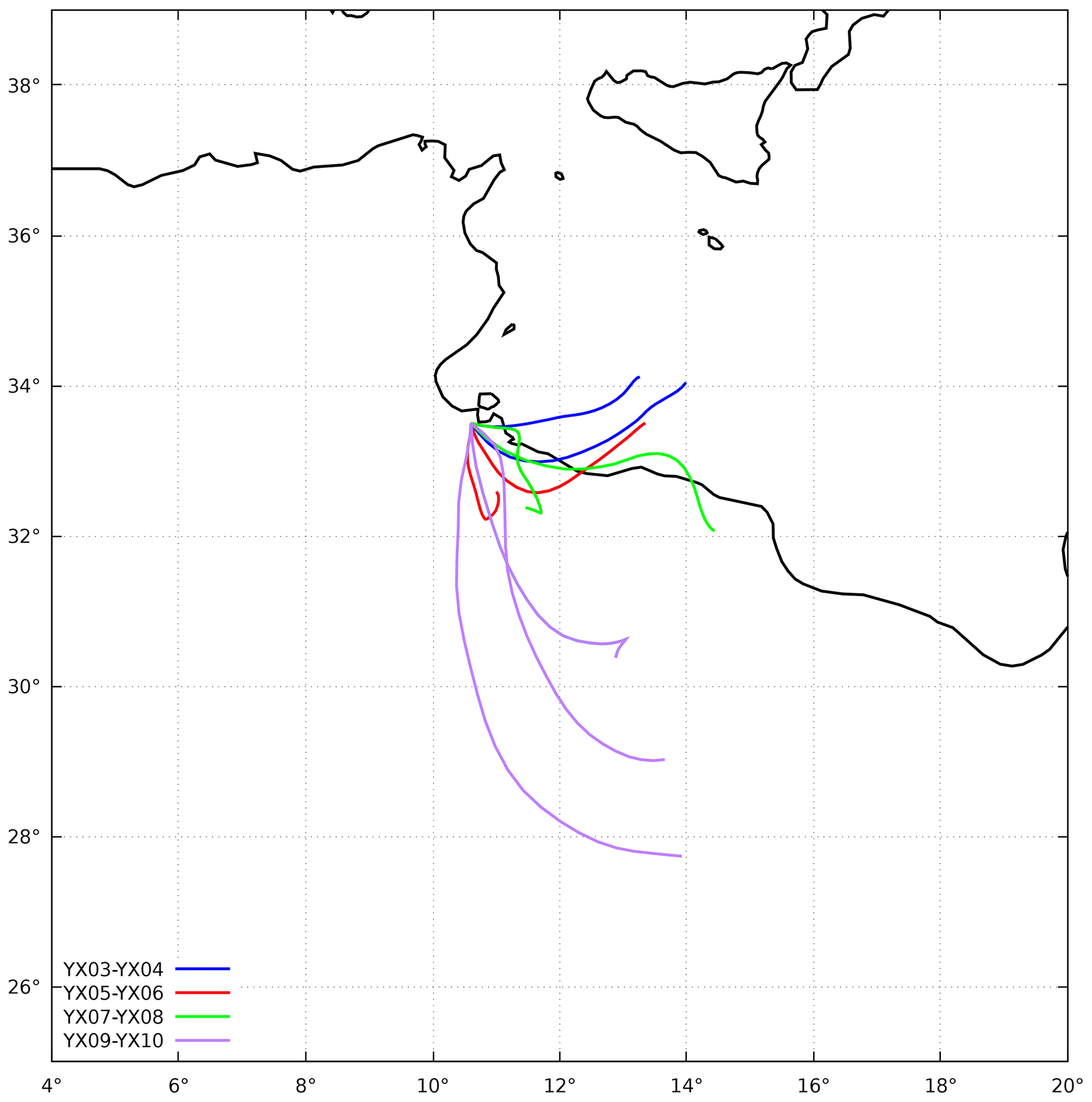
Figure C2Backward trajectories of sample pairs YX03–YX04, YX05–YX06, YX07–YX08, and YX09–YX10. The x axis is longitude, and the y axis is latitude. Two or three trajectories are associated with a given sample pair of ≈ 12 h duration.
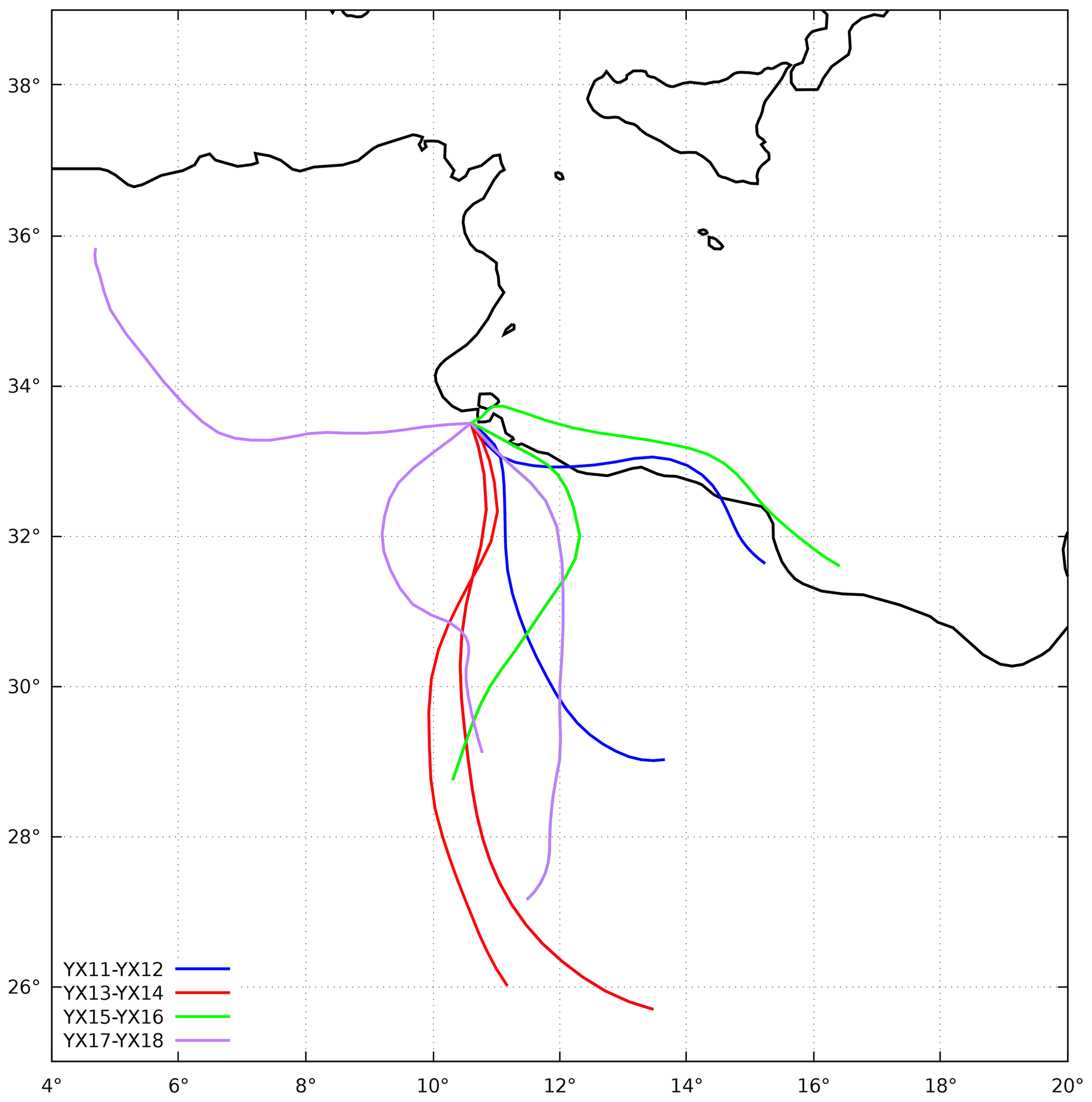
Figure C3Backward trajectories of sample pairs YX11–YX12, YX13–YX14, YX15–YX16, and YX17–YX18. The x axis is longitude, and the y axis is latitude. Two or three trajectories are associated with a given sample pair of ≈ 12 h duration.
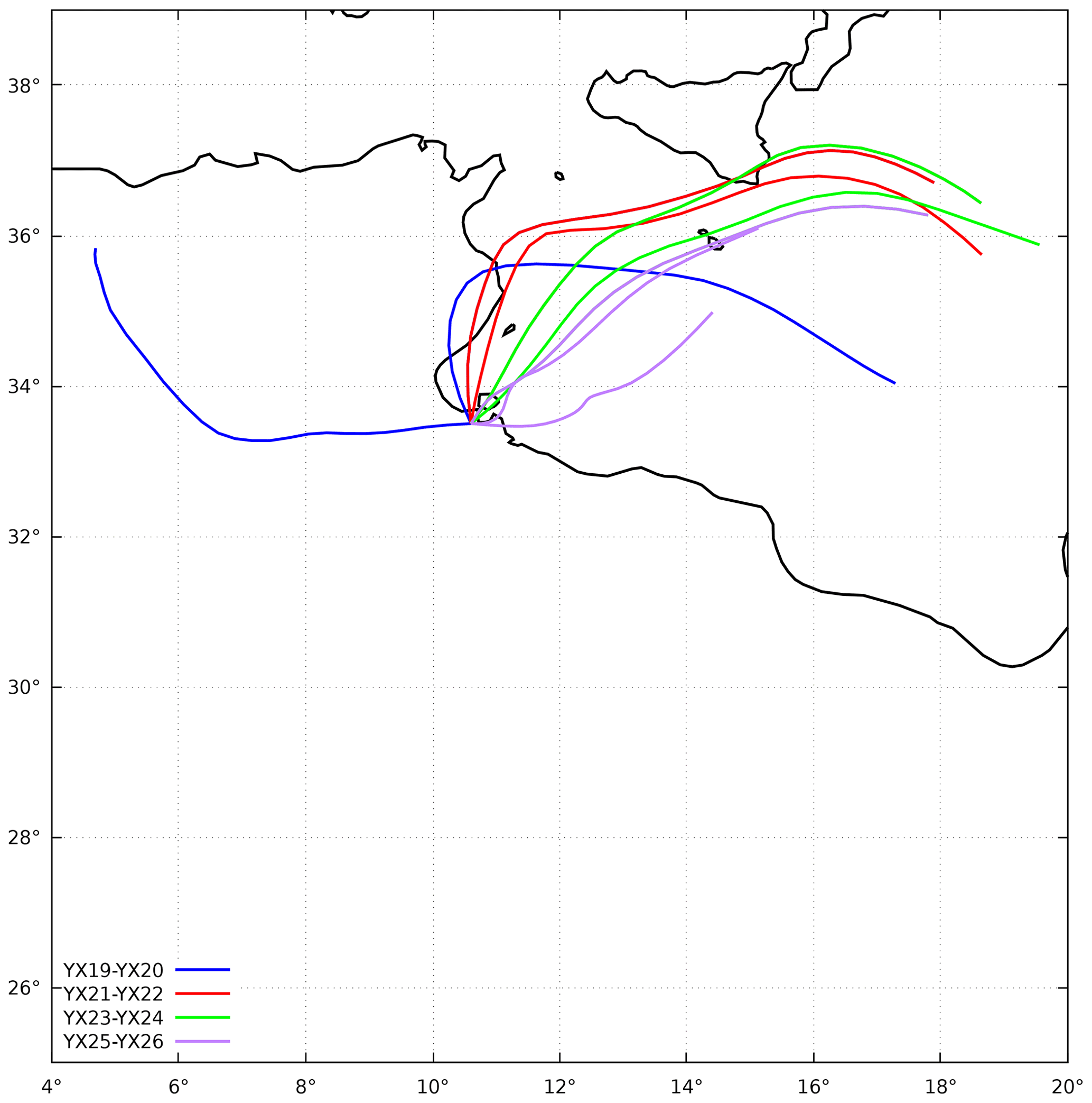
Figure C4Backward trajectories of sample pairs YX19–YX20, YX21–YX22, YX23–YX24, and YX25–YX26. The x axis is longitude, and the y axis is latitude. Two or three trajectories are associated with a given sample pair of ≈ 12 h duration.
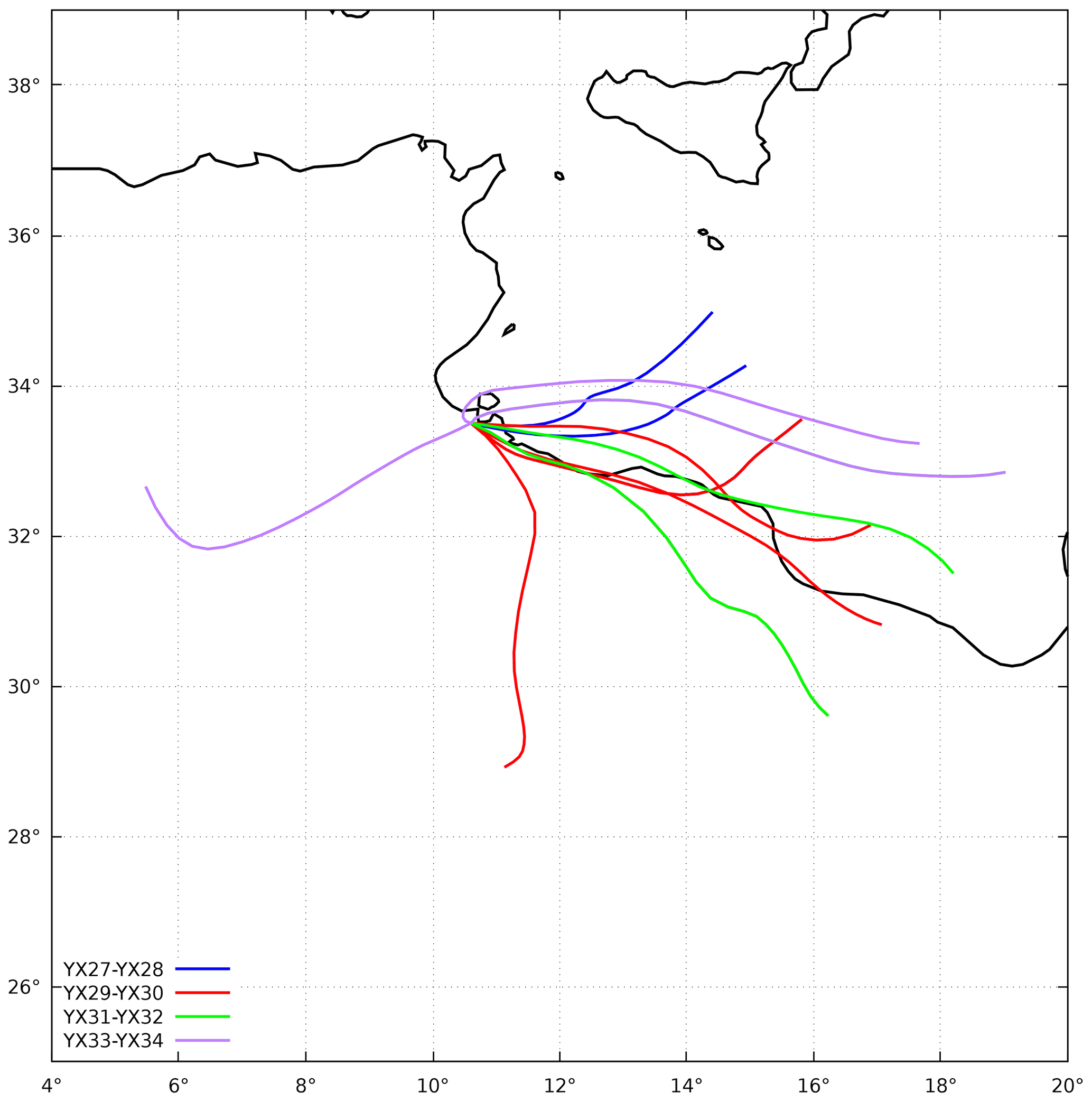
Figure C5Backward trajectories of sample pairs YX27–YX28, YX29–YX30, YX31–YX32, and YX33–YX34. The x axis is longitude, and the y axis is latitude. Two or three trajectories are associated with a given sample pair of ≈ 12 h duration, except for the pair YX29–YX30, for which four trajectories are necessary because the sampling duration was 24 h.
Table D1Optimal slope and intercept using orthogonal regressions, including the heavy loaded sample.
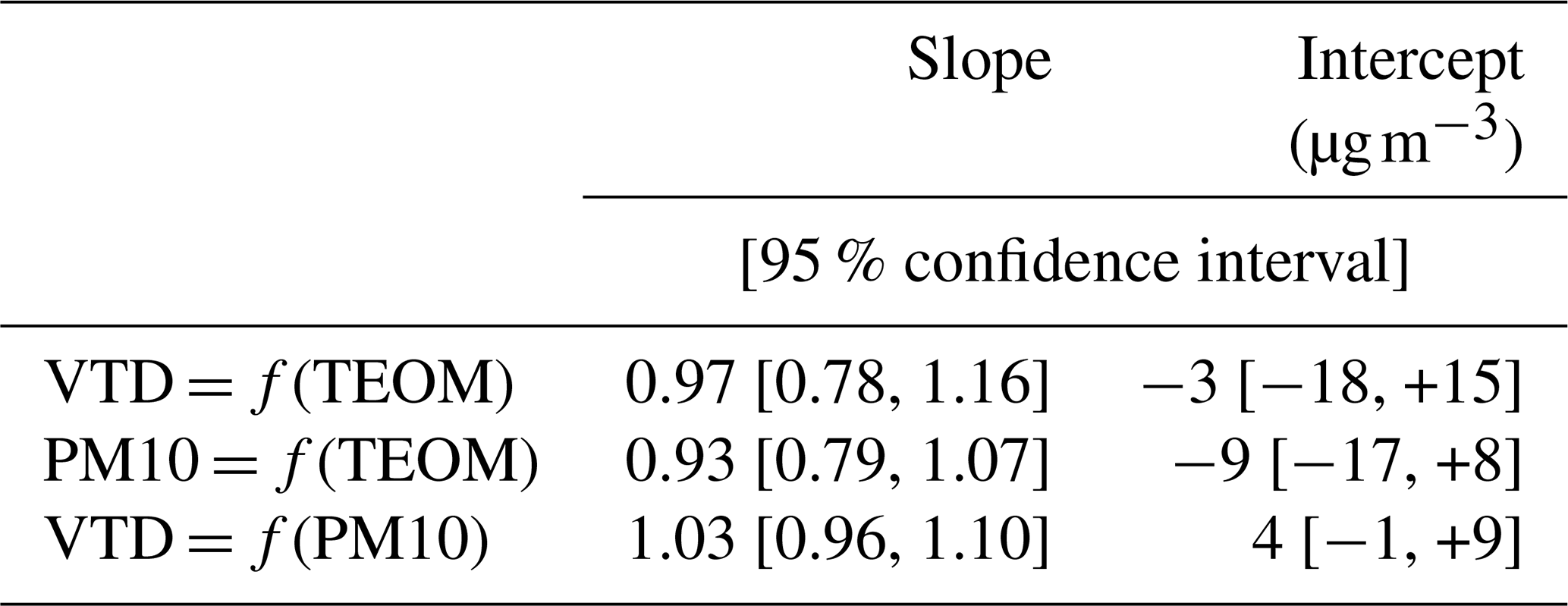
Table D2Optimal slope and intercept using orthogonal regressions, excluding the heavy loaded sample.

Table E1VTD aerosol mass concentrations derived from chemical analyses with associated analytical uncertainties (95 % confidence interval).
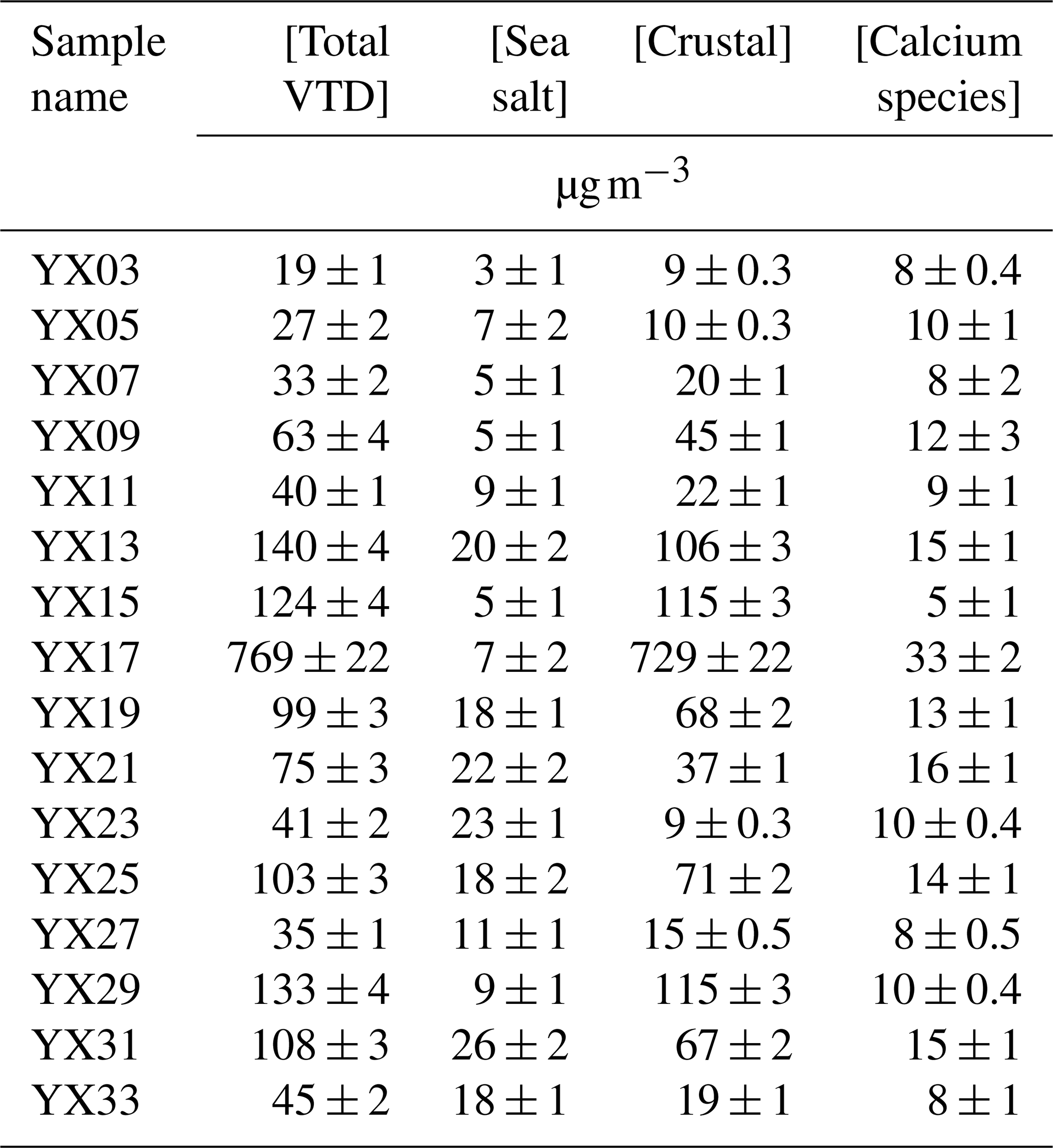
Table E2PM10 aerosol mass concentrations derived from chemical analyses with associated analytical uncertainties (95 % confidence interval).
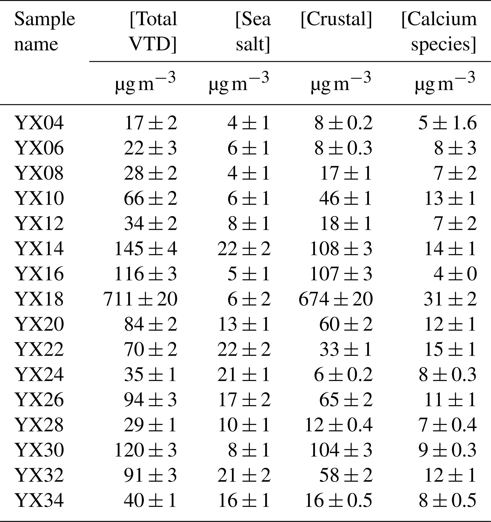
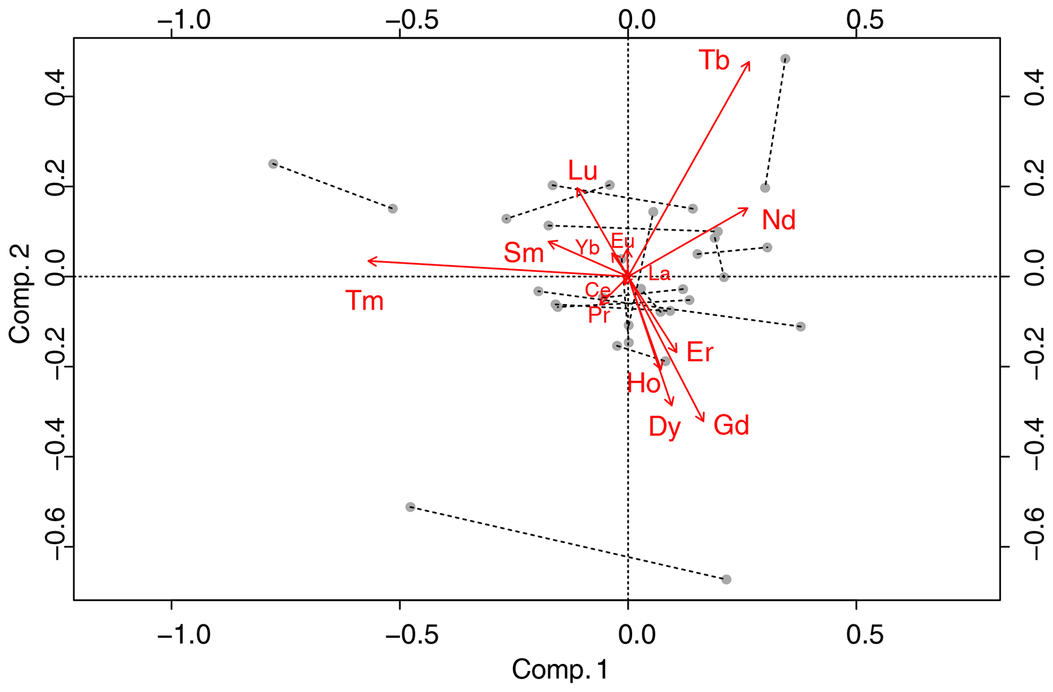
Figure F1REE biplot for two VTD simulation results. Percentages of variability explained by the first two components are 27 % and 19 %, a total of 46 %.
No other data than those presented here in tables were used in this article.
All the authors contributed to this paper to an extent, reflected by their rank in the list of authors. YXY did conceptualization, data curation, formal analysis, investigation, methodology, validation, and visualization, wrote the original draft, and conducted review and editing. RL did conceptualization, data curation, formal analysis, investigation, methodology, validation, and visualization, provided resources, and conducted review editing. FM did conceptualization, data curation, formal analysis, methodology, validation, and visualization, provided resources, and conducted review and editing. JLR did conceptualization, investigation, and methodology, provided resources, and conducted review and editing. ML did conceptualization, investigation, and methodology, provided resources, and conducted review and editing. GB did conceptualization and methodology and conducted review and editing. BM did conceptualization, methodology, and project administration, acquired funding, and conducted review and editing.
The authors declare that they have no conflict of interest.
Publisher's note: Copernicus Publications remains neutral with regard to jurisdictional claims in published maps and institutional affiliations.
We thank the Institut des Régions Arides (IRA) for providing logistics and support during the experiment. Special thanks are expressed to Thierry Henry Des Tureaux for his invaluable help during sampling in Tunisia and to Elisabeth Bon Nguyen, Mickael Tharaud, Anais Feron, Jessica Chane Teng, and Zihan Qu for their advice and help during the analyses. Thanks are given to Carmela Chateau-Smith, who reviewed the English, and to the two anonymous reviewers, who helped us to improve this paper greatly.
This work was supported by NILDAE (Nutrients Inputs and Losses Due to Aeolian Erosion in the Sahel), an IdEx Université Sorbonne Paris Cité (now Université de Paris) programme.
This paper was edited by Pierre Herckes and reviewed by two anonymous referees.
Aitchison, J.: The statistical analysis of compositional data, Chapman and Hall, London, 1986. a, b
Aitchison, J.: On criteria for measures of compositional difference, Math. Geol., 24, 365–379, 1992. a
Aitchison, J. and Ng, K. W.: The role of perturbation in compositional data analysis, Stat. Model., 5, 173–185, https://doi.org/10.1191/1471082X05st091oa, 2005. a
Aitchison, J. M.: A Concise Guide to Compositional Data Analysis, Compositional Data Analysis Workshop, CoDaWork'05, Girona Universitat de Girona, 19-21 October 2005, available at: http://ima.udg.edu/Activitats/CoDaWork05/A_concise_guide_to_compositional_data_analysis.pdf (last access: 20 November 2021), 2005. a
Alfaro, S. C. and Gomes, L.: Modeling mineral aerosol production by wind erosion: Emission intensities and aerosol size distributions in source areas, J. Geophys. Res.-Atmos., 106, 18075–18084, https://doi.org/10.1029/2000JD900339, 2001. a
Barceló-Vidal, C., Martín-Fernández, J. A., and Pawlowsky-Glahn, V.: Mathematical foundations of compositional data analysis, in: Proceedings of IAMG'01–The Sixth Annual Conference of the International Association for Mathematical Geology, edited by: Ross, G., CO-ROM, 20 pp., 2001. a
Boucher, O., Randall, D., Artaxo, P., Bretherton, C., Feingold, G., Forster, P., Kerminen, V.-M., Kondo, Y., Liao, H., Lohmann, U., Rasch, P., Satheesh, S. K., Sherwood, S., Stevens, B., and Zhang, X. Y.: Clouds and aerosols, in: Climate Change 2013: The Physical Science Basis. Contribution of Working Group I to the Fifth Assessment Report of the Intergovernmental Panel on Climate Change, edited by: Stocker, T. F., Qin, D., Plattner, G.-K., Tignor, M., Allen, S. K., Boschung, J., Nauels, A., Xia, Y., Bex, V., and Midgley, P. M., Cambridge University Press, Cambridge, United Kingdom and New York, NY, USA, https://doi.org/10.1017/CBO9781107415324.016, 571–657, 2013. a
Bowen, H. J. M.: Trace elements in biochemistry, Academic Press, London, New York, 1966. a, b
Calvert, J. G.: Glossary of atmospheric chemistry terms (Recommendations 1990), Pure Appl. Chem., 62, 2167–2219, https://doi.org/10.1351/pac199062112167, 1990. a
Chappell, A., Lee, J. A., Baddock, M., Gill, T. E., Herrick, J. E., Leys, J. F., Marticorena, B., Petherick, L., Schepanski, K., Tatarko, J., Telfer, M., and Webb, N. P.: A clarion call for aeolian research to engage with global land degradation and climate change, Aeolian Res., 32, A1–A3, https://doi.org/10.1016/j.aeolia.2018.02.007, 2018. a
Dickson, A. and Goyet, C.: Handbook of methods for the analysis of the various parameters of the carbon dioxide system in sea water. Version 2, Tech. Rep. ORNL/CDIAC–74, 10107773, U.S. Department of Energy, US, https://doi.org/10.2172/10107773, 1994. a
Egozcue, J. J., Pawlowsky-Glahn, V., Mateu-Figueras, G., and Barceló-Vidal, C.: Isometric Logratio Transformations for Compositional Data Analysis, Math. Geol., 35, 279–300, https://doi.org/10.1023/A:1023818214614, 2003. a
Faulkner, W. B., Smith, R., and Haglund, J.: Large Particle Penetration During PM10 Sampling, Aerosol Sci. Tech., 48, 676–687, https://doi.org/10.1080/02786826.2014.915005, 2014. a
Filzmoser, P., Hron, K., and Reimann, C.: Principal component analysis for compositional data with outliers, Environmetrics, 20, 621–632, https://doi.org/10.1002/env.966, 2009. a
Gabriel, K. R.: The biplot graphic display of matrices with application to principal component analysis, Biometrika, 58, 453–467, https://doi.org/10.1093/biomet/58.3.453, 1971. a
Gillette, D. A.: Production of dust that may be carried great distances, in: Geological Society of America Special Papers, Geological Society of America, 186, 11–26, https://doi.org/10.1130/SPE186-p11, 1981. a
Ginoux, P., Prospero, J., Torres, O., and Chin, M.: Long-term simulation of global dust distribution with the GOCART model: correlation with North Atlantic Oscillation, Environ. Model. Softw., 19, 113–128, https://doi.org/10.1016/S1364-8152(03)00114-2, 2004. a
Gomes, L., Bergametti, G., Coudé-Gaussen, G., and Rognon, P.: Submicron desert dusts: A sandblasting process, J. Geophys. Res., 95, 13927, https://doi.org/10.1029/JD095iD09p13927, 1990. a
Guieu, C., Loÿe-Pilot, M.-D., Ridame, C., and Thomas, C.: Chemical characterization of the Saharan dust end-member: Some biogeochemical implications for the western Mediterranean Sea, J. Geophys. Res.-Atmos., 107, ACH 5-1–ACH 5-11, https://doi.org/10.1029/2001JD000582, 2002. a
Haig, C., Mackay, W., Walker, J., and Williams, C.: Bioaerosol sampling: sampling mechanisms, bioefficiency and field studies, J. Hosp. Infect., 93, 242–255, https://doi.org/10.1016/j.jhin.2016.03.017, 2016. a
Heal, M. R., Beverland, I. J., McCabe, M., Hepburn, W., and Agius, R. M.: Intercomparison of five PM10 monitoring devices and the implications for exposure measurement in epidemiological research, J. Environ. Monitor., 2, 455–461, https://doi.org/10.1039/B002741N, 2000. a
Heimburger, A., Tharaud, M., Monna, F., Losno, R., Desboeufs, K., and Nguyen, E. B.: SLRS-5 Elemental Concentrations of Thirty-Three Uncertified Elements Deduced from SLRS-5/SLRS-4 Ratios, Geostand. Geoanal. Res., 37, 77–85, https://doi.org/10.1111/j.1751-908X.2012.00185.x, 2013. a
Hitzenberger, R., Berner, A., Galambos, Z., Maenhaut, W., Cafmeyer, J., Schwarz, J., Müller, K., Spindler, G., Wieprecht, W., Acker, K., Hillamo, R., and Mäkelä, T.: Intercomparison of methods to measure the mass concentration of the atmospheric aerosol during INTERCOMP2000 – influence of instrumentation and size cuts, Atmos. Environ., 38, 6467–6476, https://doi.org/10.1016/j.atmosenv.2004.08.025, contains Special Issue section on Measuring the composition of Particulate Matter in the EU, 2004. a
Huneeus, N., Schulz, M., Balkanski, Y., Griesfeller, J., Prospero, J., Kinne, S., Bauer, S., Boucher, O., Chin, M., Dentener, F., Diehl, T., Easter, R., Fillmore, D., Ghan, S., Ginoux, P., Grini, A., Horowitz, L., Koch, D., Krol, M. C., Landing, W., Liu, X., Mahowald, N., Miller, R., Morcrette, J.-J., Myhre, G., Penner, J., Perlwitz, J., Stier, P., Takemura, T., and Zender, C. S.: Global dust model intercomparison in AeroCom phase I, Atmos. Chem. Phys., 11, 7781–7816, https://doi.org/10.5194/acp-11-7781-2011, 2011. a
Kuklinska, K., Wolska, L., and Namiesnik, J.: Air quality policy in the U.S. and the EU – a review, Atmos. Pollut. Res., 6, 129–137, https://doi.org/10.5094/APR.2015.015, 2015. a
Le, T.-C., Shukla, K. K., Sung, J.-C., Li, Z., Yeh, H., Huang, W., and Tsai, C.-J.: Sampling efficiency of low-volume PM10 inlets with different impaction substrates, Aerosol Sci. Tech., 53, 295–308, https://doi.org/10.1080/02786826.2018.1559919, 2019. a
Mahowald, N., Ward, D. S., Kloster, S., Flanner, M. G., Heald, C. L., Heavens, N. G., Hess, P. G., Lamarque, J.-F., and Chuang, P. Y.: Aerosol Impacts on Climate and Biogeochemistry, Annu. Rev. Env. Resour., 36, 45–74, https://doi.org/10.1146/annurev-environ-042009-094507, 2011. a
Marticorena, B. and Bergametti, G.: Modeling the atmospheric dust cycle: 1. Design of a soil-derived dust emission scheme, J. Geophys. Res.-Atmos., 100, 16415–16430, https://doi.org/10.1029/95JD00690, 1995. a
Marticorena, B., Bergametti, G., Aumont, B., Callot, Y., N'Doumé, C., and Legrand, M.: Modeling the atmospheric dust cycle: 2. Simulation of Saharan dust sources, J. Geophys. Res.-Atmos., 102, 4387–4404, https://doi.org/10.1029/96JD02964, 1997. a
Mori, I., Nishikawa, M., and Iwasaka, Y.: Chemical reaction during the coagulation of ammonium sulphate and mineral particles in the atmosphere, Sci. Total Environ., 224, 87–91, https://doi.org/10.1016/S0048-9697(98)00323-4, 1998. a
Motallebi, N., Taylor, Jr., C. A., Turkiewicz, K., and Croes, B. E.: Particulate Matter in California: Part 1—Intercomparison of Several PM2.5, PM10–2.5, and PM10 Monitoring Networks, J. Air Waste Manage., 53, 1509–1516, https://doi.org/10.1080/10473289.2003.10466322, 2003. a
N'Tchayi Mbourou, G., Bertrand, J., and Nicholson, S.: The Diurnal and Seasonal Cycles of Wind-Borne Dust over Africa North of the Equator, J. Appl. Meteorol., 36, 868–882, https://doi.org/10.1175/1520-0450(1997)036<0868:TDASCO>2.0.CO;2, 1997. a
Okin, G. S., Mahowald, N., Chadwick, O. A., and Artaxo, P.: Impact of desert dust on the biogeochemistry of phosphorus in terrestrial ecosystems, Global Biogeochem. Cy., 18, GB2005, https://doi.org/10.1029/2003GB002145, 2004. a
Okin, G. S., Baker, A. R., Tegen, I., Mahowald, N. M., Dentener, F. J., Duce, R. A., Galloway, J. N., Hunter, K., Kanakidou, M., Kubilay, N., Prospero, J. M., Sarin, M., Surapipith, V., Uematsu, M., and Zhu, T.: Impacts of atmospheric nutrient deposition on marine productivity: Roles of nitrogen, phosphorus, and iron: ATMOSPHERIC DEPOSITION TO OCEANS, Global Biogeochem. Cy., 25, GB2022, https://doi.org/10.1029/2010GB003858, 2011. a
Prospero, J. M. and Nees, R. T.: Impact of the North African drought and El Niño on mineral dust in the Barbados trade winds, Nature, 320, 735–738, https://doi.org/10.1038/320735a0, 1986. a
R Core Team: R: A Language and Environment for Statistical Computing, R Foundation for Statistical Computing, Vienna, Austria, available at: http://www.R-project.org/ (last access: 29 November 2021), 2014. a
Rahn, K.: The Chemical Composition of the Atmospheric Aerosol, Tech. rep., Graduate School of Oceanography, University of Rhode Island, Kingston, Rhode Island, USA, available at: https://books.google.fr/books?hl=fr&lr=&id=q-dOAQAAMAAJ&oi=fnd&pg=PA1&dq=The+Chemical+Composition+of+the+Atmospheric+Aerosol&ots=Gz11fOEivU&sig=lYh8sJjlLtUuA5KXxST6YbXU34c#v=onepage&q=The%20Chemical%20Composition%20of%20the%20Atmospheric%20Aerosol&f=false (last access: 29 November 2021), 1976. a
Rolph, G., Stein, A., and Stunder, B.: Real-time Environmental Applications and Display sYstem: READY, Environ. Model. Softw., 95, 210–228, https://doi.org/10.1016/j.envsoft.2017.06.025, 2017. a
Scheuvens, D., Schütz, L., Kandler, K., Ebert, M., and Weinbruch, S.: Bulk composition of northern African dust and its source sediments — A compilation, Earth-Sci. Rev., 116, 170–194, https://doi.org/10.1016/j.earscirev.2012.08.005, 2013. a
Shao, Y.: Dust Emission, in: Physics and modelling of wind erosion, no. 37 in Atmospheric and oceanographic sciences library, S.l., 2. rev. & exp. ed edn., oCLC: 837050860, Springer, Netherlands, 211–245, 2008. a
Shao, Y., Raupach, M. R., and Findlater, P. A.: Effect of saltation bombardment on the entrainment of dust by wind, J. Geophys. Res., 98, 12719, https://doi.org/10.1029/93JD00396, 1993. a
Stein, A., Draxler, R., Rolph, G., Stunder, B., Cohen, M., and Ngan, F.: NOAA's HYSPLIT Atmospheric Transport and Dispersion Modeling System, B. Am. Meteorol. Soc., 96, 2059–2077, https://doi.org/10.1175/BAMS-D-14-00110.1, 2015. a
Suárez, M. H., Molina Pérez, D., Rodríguez-Rodríguez, E., Díaz Romero, C., Espinosa Borreguero, F., and Galindo-Villardón, P.: The Compositional HJ-Biplot—A New Approach to Identifying the Links among Bioactive Compounds of Tomatoes, Int. J. Mol. Sci., 17, 1828, https://doi.org/10.3390/ijms17111828, 2016. a
van den Boogaart, K., Tolosana-Delgado, R., and Bren, M.: compositions: Compositional Data Analysis. R package version 1.40-1, R-project, Vienna, Austria available at: https://CRAN.R-project.org/package=compositions (last access: 29 November 2021), 2014. a
Van der Weijden, C. H.: Pitfalls of normalization of marine geochemical data using a common divisor, Mar. Geology, 184, 167–187, https://doi.org/10.1016/S0025-3227(01)00297-3, 2002. a
Verrall, R. and Bell, R.: Square root graph paper for nuclear spectra, Nucl. Instrum. Methods, 67, 353–354, https://doi.org/10.1016/0029-554X(69)90475-3, 1969. a
von Eynatten, H., Pawlowsky-Glahn, V., and Egozcue, J. J.: Understanding Perturbation on the Simplex: A Simple Method to Better Visualize and Interpret Compositional Data in Ternary Diagrams, Math. Geol., 34, 249–257, https://doi.org/10.1023/A:1014826205533, 2002. a
Wang, G., Li, J., Ravi, S., Scott Van Pelt, R., Costa, P. J., and Dukes, D.: Tracer techniques in aeolian research: Approaches, applications, and challenges, Earth-Sci. Rev., 170, 1–16, https://doi.org/10.1016/j.earscirev.2017.05.001, 2017. a
Yu, K.-P., Chen, Y.-P., Gong, J.-Y., Chen, Y.-C., and Cheng, C.-C.: Improving the collection efficiency of the liquid impinger for ultrafine particles and viral aerosols by applying granular bed filtration, J. Aerosol Sci., 101, 133–143, https://doi.org/10.1016/j.jaerosci.2016.08.002, 2016. a
- Abstract
- Introduction
- Materials and methods
- Results and discussion
- Conclusions
- Appendix A: Air concentrations, measured values
- Appendix B: Geostandard recovery rates
- Appendix C: Local meteorological conditions and air trajectories
- Appendix D: Mass comparison statistical parameters
- Appendix E: Detailed mass calculations for VTD and PM10
- Appendix F: REE biplot simulated with the observed analytical uncertainty.
- Data availability
- Author contributions
- Competing interests
- Disclaimer
- Acknowledgements
- Financial support
- Review statement
- References
The requested paper has a corresponding corrigendum published. Please read the corrigendum first before downloading the article.
- Article
(2953 KB) - Full-text XML
- Abstract
- Introduction
- Materials and methods
- Results and discussion
- Conclusions
- Appendix A: Air concentrations, measured values
- Appendix B: Geostandard recovery rates
- Appendix C: Local meteorological conditions and air trajectories
- Appendix D: Mass comparison statistical parameters
- Appendix E: Detailed mass calculations for VTD and PM10
- Appendix F: REE biplot simulated with the observed analytical uncertainty.
- Data availability
- Author contributions
- Competing interests
- Disclaimer
- Acknowledgements
- Financial support
- Review statement
- References