the Creative Commons Attribution 4.0 License.
the Creative Commons Attribution 4.0 License.
 | 08 Dec 2021
Idealized simulation study of the relationship of disdrometer sampling statistics with the precision of precipitation rate measurement
Due to the discretized nature of rain, the measurement of a continuous precipitation rate by disdrometers is subject to statistical sampling errors. Here, Monte Carlo simulations are employed to obtain the precision of rain detection and rate as a function of disdrometer collection area and compared with World Meteorological Organization guidelines for a 1 min sample interval and 95 % probability. To meet these requirements, simulations suggest that measurements of light rain with rain rates R ≤ 0.50 mm h−1 require a collection area of at least 6 cm × 6 cm, and for R = 1 mm h−1, the minimum collection area is 13 cm × 13 cm. For R = 0.01 mm h−1, a collection area of 2 cm × 2 cm is sufficient to detect a single drop. Simulations are compared with field measurements using a new hotplate device, the Differential Emissivity Imaging Disdrometer. The field results suggest an even larger plate may be required to meet the stated accuracy, likely in part due to non-Poissonian hydrometeor clustering.
- Article
(4350 KB) - Full-text XML
- BibTeX
- EndNote


Ground-based precipitation sensors are commonly used to validate remotely sensed precipitation measurement systems, including satellite (TRMM), WSR-88D radar measurements (Kummerow et al., 2000; Fulton et al., 1998), and numerical weather prediction models (Colle et al., 2005) aimed at hydrology, agriculture, transportation, and recreation applications (WMO, 2018; Estévez et al., 2011; Campbell and Langevin, 1995; Brun et al., 1992). The ability of an automated weather station to detect the presence of light precipitation can be crucial for weather forecasting in remote locations where a human observer is not available to verify the presence of rainfall (Horel et al., 2002; Miller and Barth, 2003). Light rain or drizzle can severely impede road safety (Andrey and Yagar, 1993; Andrey and Mills, 2003; Bergel-Hayat et al., 2013; Theofilatos and Yannis, 2014).
Disdrometers measure particle drop size distributions and provide calculated precipitation rate from the integrated mass flux. Among available disdrometers are the mechanical Joss–Waldvogel (JW) disdrometer (Joss and Waldvogel, 1967), laser or optical sensors such as the OTT Parsivel2 (Tokay et al., 2013; Bartholomew, 2014), and video disdrometers such as the 2DVD (Kruger and Krajewski, 2002; Thurai et al., 2011; Brandes et al., 2007). In instrument development, striking a balance between sampling area and accurate fine-scale precipitation detection is a well-known problem. Among other instrument-specific considerations, disdrometer accuracy depends on the sampling area and time interval. Gultepe (2008) highlights a universal difficulty in accurately measuring very light precipitation. In their study, they compared different co-located precipitation sensors and found large absolute and relative errors (32 %–44 %) for all instruments when precipitation rate R < 0.3 mm h−1, but the relative errors were approximately 10 % when R > 1.5 mm h−1. Despite these observations, they found that optical and hotplate disdrometers can more accurately detect light precipitation compared to weighing gauges, despite having comparatively small sampling areas, typically 50 cm2, where the VRG101 weighing gauge sampling area is 400 cm2. Here, we focus solely on the effect of disdrometer sampling area and time interval on the precision of precipitation rate measurement distinct from any other uncertainties associated with the instruments themselves.
The World Meteorological Organization (WMO) recommends that a disdrometer measure precipitation with an output averaging time of 1 min (WMO, 2018). Measurement uncertainty is defined as “the uncertainty of the reported value with respect to the true value and indicates the interval in which the true value lies within a stated probability” specified to be 95 %. For liquid precipitation intensity, the uncertainty requirements for rates of 0.2 to 2 mm h−1 are ±0.1 mm h−1, and for precipitation rates > 2 mm h−1 they are 5 % (see Table 1). For < 0.2 mm h−1, the requirement is only detection.
Most commercial instruments do not reach such strict standards. Table 1 provides the reported uncertainties for several precipitation instruments. The instrumentation used by Automated Surface Observing Systems (ASOS) weather stations located at major airports utilizes a heated tipping bucket (HTB) for precipitation accumulation and a light-emitting diode weather identifier (LEDWI) for precipitation type and intensity. The LEDWI uses signal power return to determine the drop size distribution of rain or snow and then classifies the precipitation intensity based on the size distribution (Nadolski, 1998). A significant limitation of the ASOS system is that it cannot discriminate drizzle from light rain, and it qualitatively expresses small amounts as a trace (Wade, 2003; Nadolski, 1998).
Vaisala manufactures a range of optical precipitation sensors that detect and categorize precipitation from the forward scattering of a light beam, including the PWD12, PWD22, PWD52, and FD71P. The PWD12 detects rain, snow, unknown precipitation, drizzle, fog, and haze. The PWD22 has the same resolution and accuracy as the PWD12, but it also detects freezing drizzle, freezing rain, and ice pellets (Vaisala, 2019b). The PWD52 has an increased observation range of 50 km compared to 20 km for the PWD22 (Vaisala, 2018a). All three PWD instruments have a precipitation intensity resolution of 0.05 mm h−1 for a 10 min sampling interval at 10 % uncertainty (Vaisala, 2019b). The PWD22 is included with tactical weather instrumentation intended for US military and aviation operations (TACMET) and reports precipitation type in WMO METAR code format (Vaisala, 2018b). The FD71P has a higher stated sampling frequency and resolution than the PWD instruments of 0.01 mm h−1 with 2.2 % uncertainty in a 5 s measurement cycle (Vaisala, 2019a), although there has yet to be independent scientific evaluation of the device.
Hotplate disdrometers offer an alternative with the advantage of requiring fewer assumptions as mass is inferred from the energy required for evaporation. The Yankee Environmental Systems TPS-3100 determines the liquid water precipitation rate of rain or snow by taking the power difference between upward- and downward-facing hotplates as a measure of the latent heat energy required to evaporate precipitation (Rasmussen et al., 2010). The technology is currently marketed as the Pond Engineering Laboratories K63 Hotplate Total Precipitation Gauge (Pond Engineering, 2020). The hotplate is 5 in. in diameter, or 126.7 cm2, which is equivalent to a square with a width of 11.26 cm. It measures precipitation rate with a resolution of 0.10 ± 0.5 mm h−1 and can detect the onset of light snow within 1 min (Yankee Environmental Systems, 2011; Pond Engineering, 2020).
Table 1Precipitation measurement instrument specifications.

* Whichever is greater.
A newer hotplate disdrometer, yet to be commercialized, is the Differential Emissivity Imaging Disdrometer (DEID) developed at the University of Utah. The DEID measures the mass of individual hydrometeors using a hotplate and a thermal camera, which provide accurate, fine-scale measurements. A larger hotplate sampling area increases the operating cost through higher power consumption. The work here was originally motivated by a desire to minimize DEID power and maximize measurement precision, although the calculations are applicable more generally to other disdrometers such as those described. We employ a Monte Carlo approach (Liu et al., 2012, 2018; Jameson and Kostinski, 1999, 2001a, 2002) to stochastically generate raindrops based on canonical size distributions aimed at determining the minimum required disdrometer collection area and sampling frequency for precise measurement of precipitation rates between 0.01 and 10 mm h−1. We consider the precipitation rate uncertainty relative to WMO standards. Inherent precipitation measurement uncertainties associated with the instrument mechanism are not addressed here. Where Joss and Waldvogel (1969) approached the problem analytically by assuming the interarrival times of droplets up to 6 mm in diameter are distributed according to a Poisson distribution, here we approach the problem numerically by employing a Monte Carlo approach. In principle, the results should converge, although the Monte Carlo approach also facilitates the calculation here of the time required to measure the “first drop” in a precipitation event. Joss and Waldvogel (1969) defined a sample size as the product of an area and a sample time. Under the assumption that raindrop size follows an exponential distribution, to measure a precipitation rate of R = 1 mm h−1 to a precision of 10 % within 95 % confidence bounds, the required sample size is 1.5 m2 s, corresponding to a cross-sectional sampling area of A = 250 cm2 with a square sampling area width W = 15.8 cm for a nominal 60 s collection interval. The required square width W found in this work for the same parameters is 13 cm.
The DEID obtains the mass of individual precipitation particles by assuming conservation of energy during heat transfer from a square plate to a melting hydrometeor. To determine particle size during evaporation, a thermal camera is directed at a heated aluminum sheet. Since aluminum is a thermal reflector (thermal emissivity ϵ≈0.03), whereas water is not (ϵ≈0.96), particles have high brightness temperature and appear as white regions on a low brightness temperature, black background. From the measured cross-sectional surface area, temperature, and evaporation time of each hydrometeor, the effective diameter and volume and the mass of each particle can be calculated with high precision (Singh et al., 2021). A piece of polyimide tape with ϵ≈0.95 is placed on the side of the sampling area as a reference for the differential emissivity calculation and determination of the camera's pixel resolution. For the study described here, the DEID's aluminum plate had an area of 15.24 cm × 15.24 cm, and the camera pixel resolution was 0.2 mm. Polyimide tape applied to the surface restricted the collection area to A ≈ 7 cm × 5 cm, equivalent to a square width of W = 5.8 cm. Thermal camera imagery with a sampling frequency between 2 and 60 Hz was used to determine the cross-sectional surface area, temperature, and evaporation time of each hydrometeor (Singh et al., 2021). From these parameters, individual hydrometeor mass is calculated from conservation of energy, whereby the heat gained by the hydrometeor is equal to the heat lost by the hotplate when evaporating water through
where cp is the specific heat capacity of water at constant pressure, ΔT is the difference in temperature between 0 and time t, m is the mass of the hydrometeor, and Leqv is the equivalent latent heat required for the conversion of the hydrometeor to gas. For liquid precipitation Leqv=Lv, where Lv is the latent heat of vaporization of water. K is the thermal conductivity of the plate, H is hotplate thickness, A(t) is the area of the water droplet at time t, Tp is the temperature of the hotplate, and Tw(t) is the temperature of the water at time t.
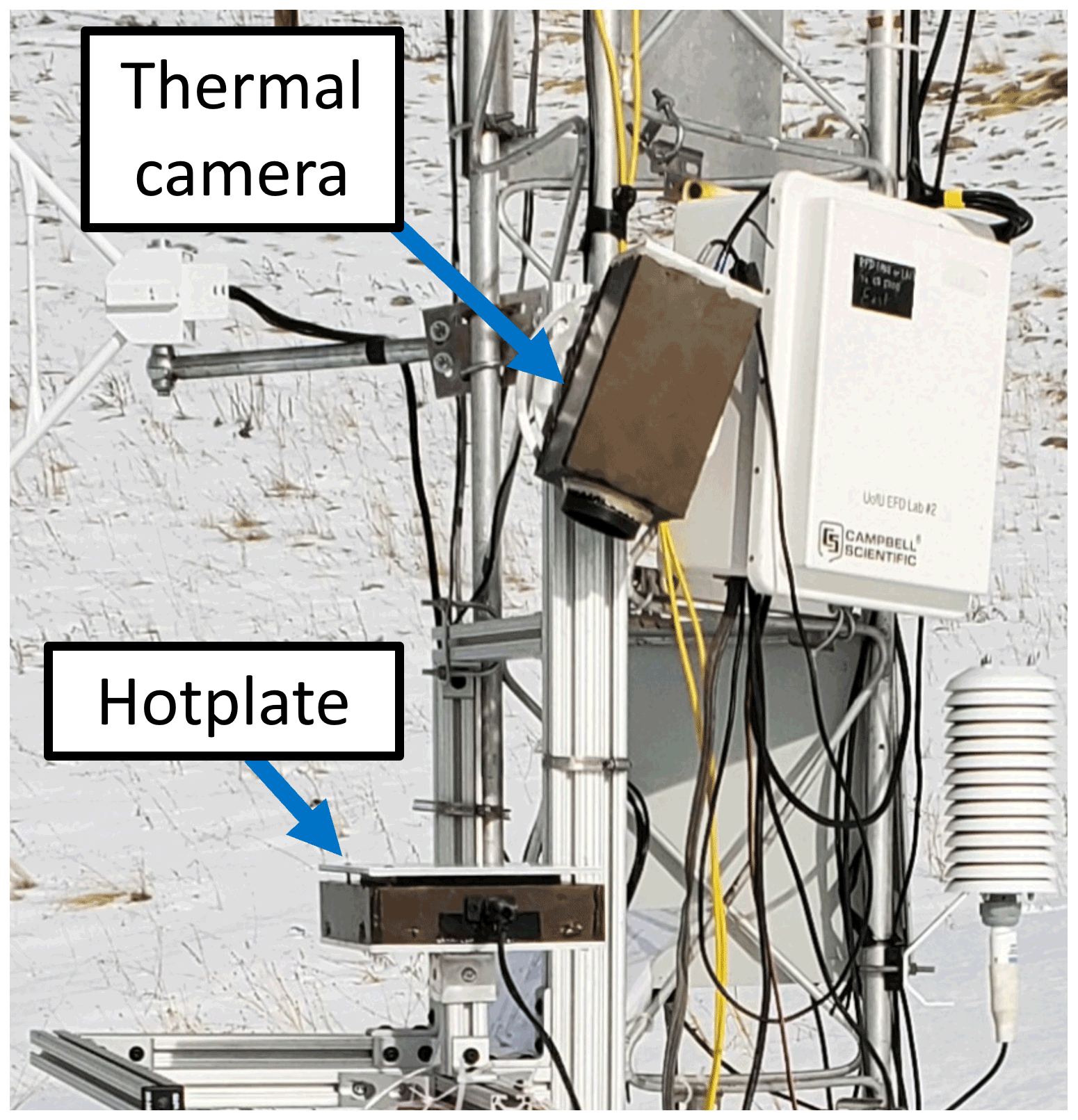
Figure 1Photograph of the DEID during the Red Butte field experiment in Salt Lake City, Utah, with the thermal camera pointed at the hotplate surface.
When combining the constants into a single value Kd, Eq. (1) simplifies to
where Kd is determined experimentally.
The precipitation rate RDEID is calculated from the total mass of hydrometeors evaporated on the hotplate during a given sample time interval. For each frame of the hotplate captured by the thermal camera,
where β = 3.6×106 mm s m−1 h−1, fs is the camera resolution (frame s−1), Aevap is the total area of water on the sampling area (m2), Imean is the pixel intensity related to the temperature difference between the plate and water through , ρw is the density of water (1000 kg m−3), and Ahot is the hotplate area (m2).
Table 2Minimum collection area required to meet WMO precision criteria for various precipitation rates and time intervals evaluated within 1 cm intervals.
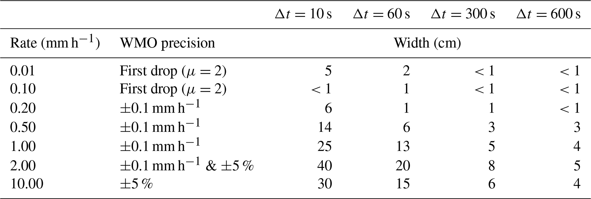
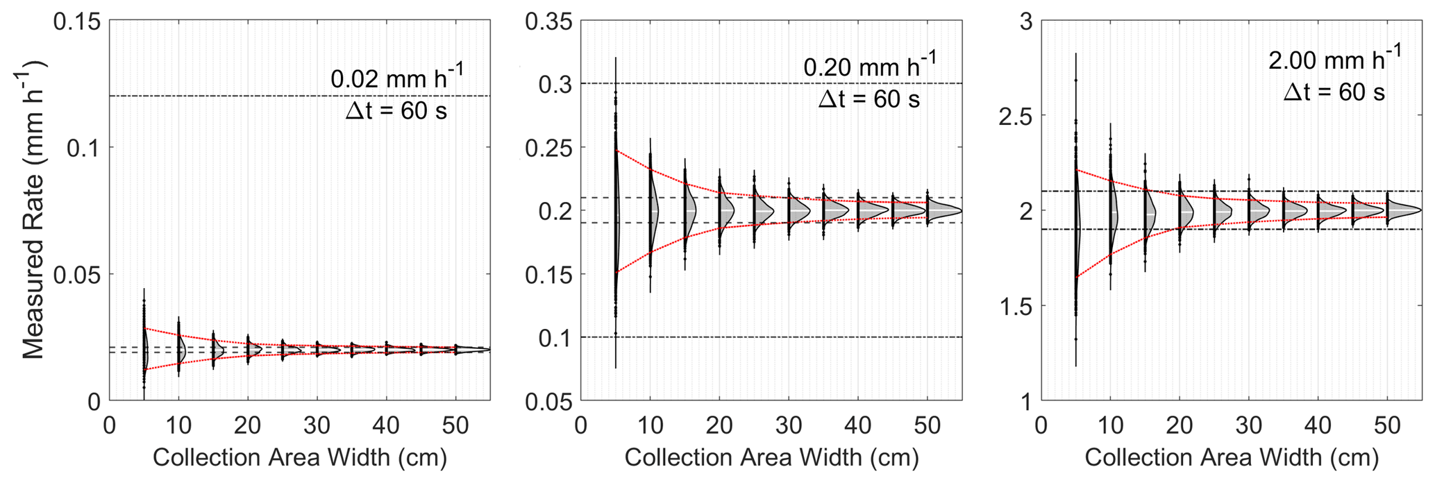
Figure 2Precipitation rate Rcalc calculated 1000 times for each W with a uniformly distributed random selection of particle sizes from the Marshall–Palmer distribution with diameters up to 6 mm for Δt = 60 s. Vertical curves represent a probability density function (PDF) of calculated Rcalc with the widths scaled according to the widest curve; 95th and 5th percentile bounds are smoothed and shown in red, dotted lines. WMO standards (±5 %, dashed, and ±0.1 mm h−1, dot-dashed) are shown as horizontal lines. The intersection of these lines indicates the required square disdrometer sampling area width to determine R according to WMO standards.
Hydrometeor catch inefficiency is a large contributor to precipitation rate measurement error, especially in bucket-type precipitation gauges (Pollock et al., 2018). Rasmussen et al. (2010) found that the Yankee hotplate had a catch efficiency of only 50 % with a wind speed of 5 m s−1 and 35 % with a wind speed of 8 m s−1. The DEID underwent a series of calibration wind tunnel tests to determine the effect of wind on mass measurements. During these experiments, mass measurements remained approximately constant, revealing that catch inefficiency is not a contributor to the precipitation rate measurement (Singh et al., 2021). The high catch efficiency from the DEID was demonstrated during a storm that took place at Alta, UT, on 16 April 2020 between 00:00 and 16:00 UTC (Fig. 10 of Singh et al., 2021). The co-located weighing gauge was located inside of a wind fence, while the DEID was not. Despite wind speeds during the storm ranging from 4 to 13 m s−1 sustained with 8–19 m s−1 gusts, DEID precipitation measurements were within 6 % of the co-located weighing gauge. For this reason, precipitation rate as a function of catch efficiency is not explored in this work.
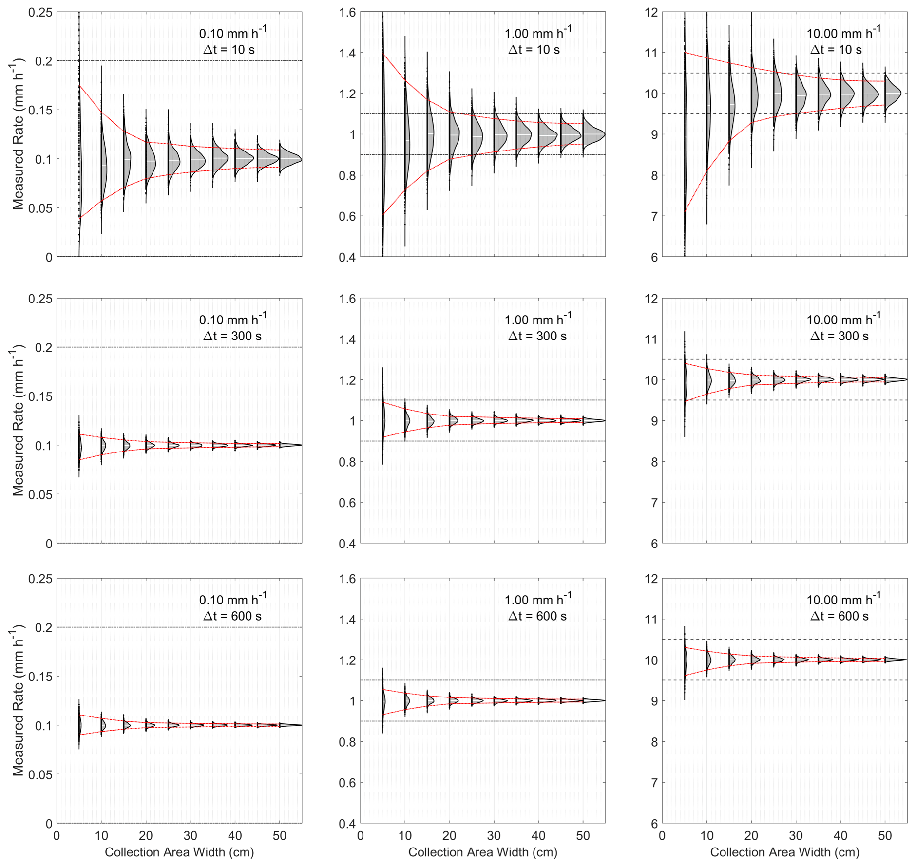
Figure 3Comparison of R = 0.10, 1.00, and 10.00 mm h−1 for Δt = 10 s, 5 min, and 10 min. The applicable WMO standards for each rate (±5 %, dashed, and ±0.1 mm h−1, dot-dashed) are shown as horizontal lines.
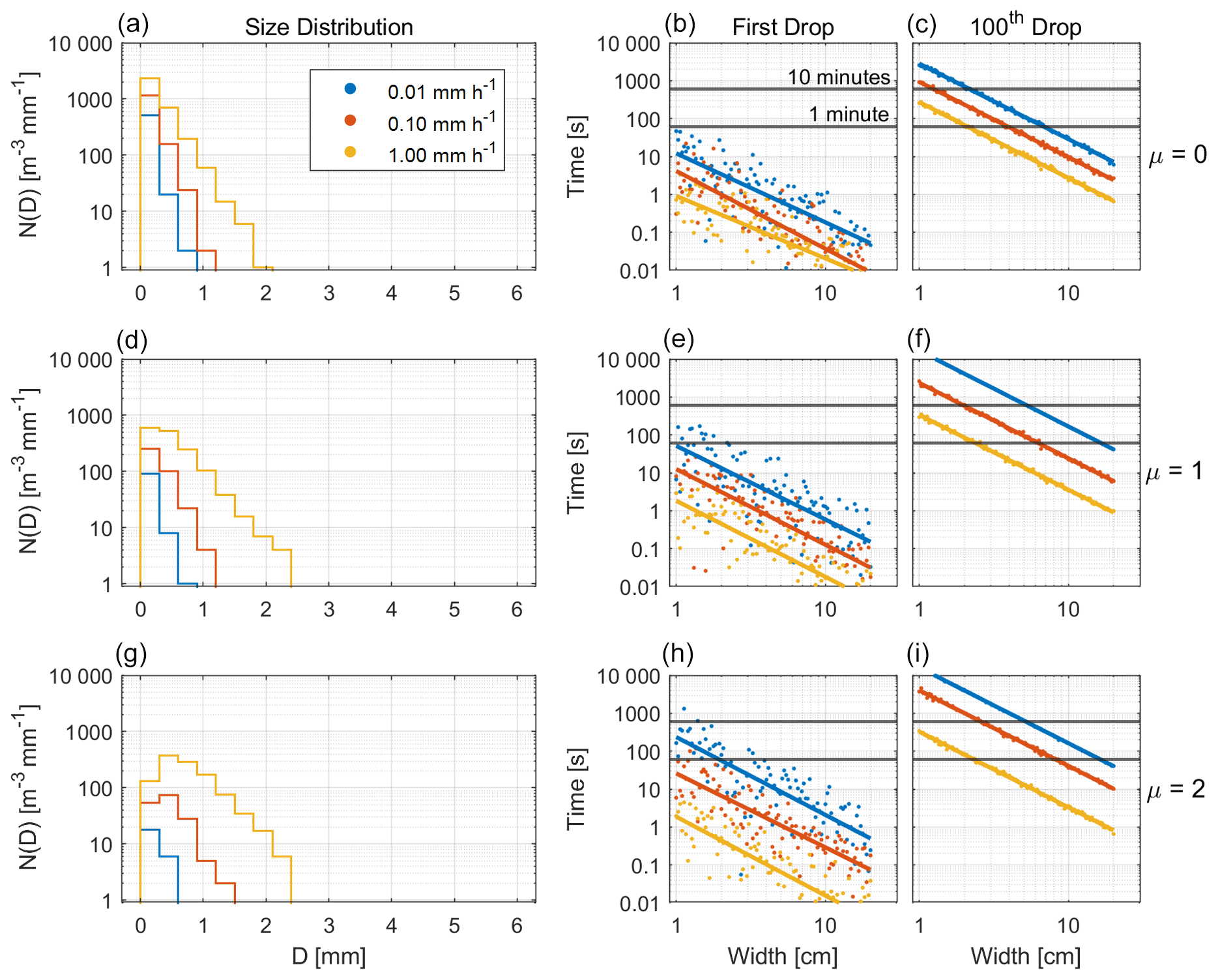
Figure 4Generated size distributions (a, d, g), first drop simulation (b, e, h), and 100th drop simulation (c, f, i) for μ = 0, 1, and 2 (top, middle, and bottom).
3.1 Size distribution generation
For a range of collection areas A and time intervals Δt, a raindrop distribution is generated stochastically and compared with the assumed rate R. Initially, we adopt the Marshall–Palmer (Marshall and Palmer, 1948) drop size distribution
where n0 = 8000 m−3 mm−1 and mm−1. D ranges between 0 and Dmax in linear bins evenly spaced by ΔD. We establish Dmax = 6 mm to account for the expected breakup of large raindrops (Villermaux and Bossa, 2009) and ΔD = 0.25 mm for 50 bins. The value of ΔD is arbitrary but was chosen to approximate the spatial measurement resolution of the prototype DEID. For an assumed value of R, the array of drops is stochastically generated according to Eq. (4), where is the total number of drops generated from each bin. Each drop in the bin is assigned a diameter of . For each value of Dmean, the fall speed is
where the coefficient a and the exponent b are determined for the Stokes regime for Dmean ≤ 0.08 mm, the intermediate regime for 0.08 mm ≤ Dmean<1.2 mm, and the turbulent regime for Dmean ≥ 1.2 mm following Lamb and Verlinde (2011). The maximum value of v is used to determine the sample volume of the generated Marshall–Palmer distribution of drops vmaxAΔt m3.
The calculated size distribution of drops incident on the collection area during sampling time Δt is then
with units of mm−1. The total calculated number of drops Ncoll incident on the collection area is a summation of Eq. (6) over the range 0 to Dmax.
3.2 Calculated precipitation rate
Ncoll drops are randomly sampled assuming the Marshall–Palmer distribution. From the drops that impact the collection area, the calculated precipitation rate Rcalc is (cf. Lane et al., 2009)
where α = 3.6 m2 s mm−2 h−1 and Ni is the number of drops with diameter Di, with i corresponding to bin number; 100 simulations of Rcalc are performed for each value of equivalent sampling area width , each evenly spaced by 1 cm. The 95th and 5th percentile bounds of Rcalc are specified as the upper and lower bounds of sampling uncertainty ().
3.3 First and hundredth drops
To determine the sampling time required to detect the onset of precipitation, 100 simulations were performed for R = 0.01, 0.1, and 1 mm h−1 and for 100 evenly spaced width bins W between 1 and 20 cm. For each width bin, the number size distribution was calculated from n(D) for a 1 m3 volume directly above the collection area with height . A sample of drops is generated from Eq. (6). To ensure that the drop with the smallest size Dmean could feasibly fall from the top to the bottom of the sample volume, is maximized using the fall speed of the minimum value of Dmean. In general, small drops contribute negligibly to calculations of precipitation rate (Smith et al., 2003), but due to their higher concentrations they may nonetheless be the first detected. Accordingly, the functional form of n(D) is adjusted from the simpler exponential form described by Eq. (4) to a gamma distribution
So that small particles with D<1 mm are not over-represented (Ulbrich and Atlas, 1984), the drop size distribution is modified by the shape parameter μ and generated according to Eq. (6). Each drop is assigned a random height Δz above the collection area within a distance h above the plate, and the time elapsed for the plate to detect a drop is . The shortest of these times is the first drop detection time t1.
Following the collection approach taken by Marshall et al. (1947), reproduction of the Marshall–Palmer size distribution is assumed to require collection of 100 drops. The time elapsed for the calculated incidence of 100 drops is t100. If fewer than 100 drops were obtained in Ncoll, a new sample of drops is obtained from Eq. (6) with an increased value of Δt.

Figure 5Recalculation of Rcalc (Eq. 7) from 1000 uniformly distributed, randomly sampled iterations of a 1 min DEID dataset from 8 March 2020 at 14:43 MST with rain rate RDEID = 4.2 mm h−1 (a). Rcalc was recalculated using uniformly distributed random segments of time (c) and hotplate sampling area width (d). As t→60 and W→WDEID, Rcalc approaches RDEID.
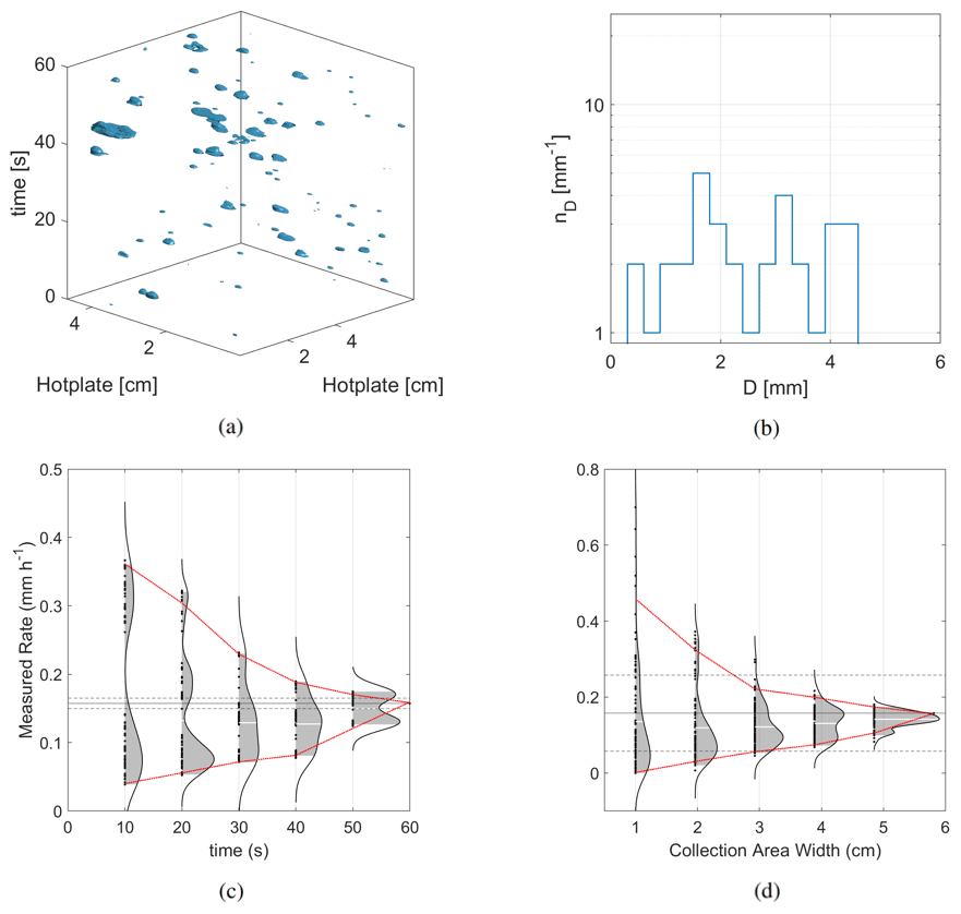
Figure 6Recalculation of Rcalc from 1000 iterations of a 1 min DEID dataset from 8 March 2020 at 15:14 MST with rain rate RDEID = 0.1 mm h−1 (a). Rcalc was calculated using uniformly distributed random segments of time (c) and hotplate sampling area width (d). As t→60 and W→WDEID, Rcalc approaches RDEID.
4.1 Monte Carlo simulations
The sampling uncertainty in the precipitation rate is illustrated in Fig. 2. Precipitation rates of R = 0.02, 0.20, and 2.00 mm h−1 were analyzed for a standard sampling time of 60 s. Collection areas smaller than approximately 6 cm × 6 cm meet WMO standards for R ≤ 0.50 mm h−1, but a collection area of over 10 cm × 10 cm is required for R> 1 mm h−1.
To illustrate the relationship between accuracy and sampling time, Fig. 3 compares R = 0.10, 1.00, and 10.00 mm h−1 with sampling times of 10 s, 5 min, and 10 min. For heavy rain rates of 10 mm h−1, for a time interval of 5 min, a disdrometer sampling area width of 4 cm yields measured rain rates with a precision of ±5 % error for 95 % of the measurements. The intersection between 95th and 5th percentile bounds and WMO accuracy criteria occurs in larger collection areas as R increases.
First drop simulation results are shown in Fig. 4. Three simulations were performed using three values of μ, where μ=0 represents the Marshall–Palmer exponential distribution and closely represents the distributions generated by the uncertainty simulations. Following Ulbrich and Atlas (1984), DEID measurements show values of μ between 1 and 2 best represent the distribution of drops that arrive on the hotplate (Figs. 5b and 6b). Monte Carlo calculations of the size distribution Ncoll are shown in Fig. 4. Note that the size distribution for N(D)coll does not converge to N(D)MP for long sampling times because smaller drops fall slowly. Rather, the distribution more closely resembles a gamma distribution (Ulbrich and Atlas, 1984). Nevertheless, the contribution of small drops to ground-based measurements of precipitation tends to be small as they are comparatively less massive. Also, precipitation particles form primarily from droplet collisions in the updrafts within clouds and so must attain the size that they fall sufficiently quickly to leave cloud base and fall to the ground where they can be sampled by ground-based instruments (Garrett, 2019). For μ = 2, few of the smallest drops with D<1 mm are incident on the collection area. A square collection sampling area width of 2 cm × 2 cm is sufficient to detect the onset of light precipitation with a rate of R=0.01 mm h−1 within 1 min.
4.2 Application to DEID measurements
During a field campaign that took place at the University of Utah between April 2019 and March 2020, the DEID recorded the mass and density of individual hydrometeors, along with the 1 min-averaged precipitation rate RDEID for six rain events and five snow events with data spanning 1185 total minutes. DEID particle mass distributions for two contrasting 1 min samples of convective moderate (RDEID = 4.2 mm h−1) and light (RDEID = 0.1 mm h−1) rain are shown in Figs. 5 and 6. These samples were selected from rain-only events with measured RDEID values closest to the values of R that were analyzed in Sect. 4.1. These disdrometer data are used here in place of an assumed size distribution to calculate Rcalc (Eq. 7) in 100 iterations, each taken from data randomly sampled over time interval segments of Δt = 10, 20, 30, 40, and 50 s (Figs. 5c and 6c) and plate area segments of W = 1, 2, 3, 4, and 5 cm (Figs. 5d and 6d). Segments of Δt include all particles within the DEID collection area, and segments in W encompass the entire 60 s time interval. In a three-dimensional space of plate cross-sectional area and sampling time, the associated number concentration of drops for each case is shown in Figs. 5a–b and 6a–b.
The version of the DEID used in this study had a maximum collection area width of W = 5.8 cm. For moderate rain where R = 1 mm h−1, the derived minimum required sampling area width to meet WMO requirements is 13 cm. That is, the size of plate used was insufficient for the measurement of rain this intense. For light rain, the statistical uncertainty bounds at 95 % confidence converge to within ±0.1 mm h−1 of the DEID 1 min measured rate for a plate collection area width of W ∼ 3 cm. This value is larger than the 2 cm suggested by the Monte Carlo calculation shown in Table 2. One possibility is that the raindrop interarrival time and spacing were not in fact Poissonian (Jameson and Kostinski, 2001b). In the event of clustering, a larger plate would be required to provide an accurate assessment of the average rain rate during a given time interval.
To assess whether the presence of non-Poissonian clustering is the case, two-point correlation functions η were calculated following Shaw et al. (2002). A value of unity indicates interarrival times that are Poissonian and values greater than unity the presence of non-random clustering. Based on the location of hydrometeor centroids as they arrive on the DEID plate, storm-averaged values of η were found to be equal to 1.01 for rain falling under light winds on 8 March 2020, between 13:38 and 15:49 MST, and equal to 1.10 for the period between 05:00 and 07:34 MST earlier that day when high winds were present. For contrast, the value of η was 1.55 for a snow event with large aggregate snowflakes that took place on 14 January 2020 at 12:43–14:06 MST. While more extensive analysis is required, the implication is that non-Poissonian clustering can occur.
A Monte Carlo approach was used to determine the minimum required cross-sectional collection area for a disdrometer to measure a given precipitation rate with a WMO target precision at 95 % probability for a 1 min collection period. Intrinsic instrument uncertainties were not considered, only those associated with statistical sampling errors associated with the raindrop size distribution. Following these criteria, a square collection area of 6 cm × 6 cm is sufficient to detect the onset of light rain with R ≤ 0.50 mm h−1.
For R>1 mm h−1, a sample area of over 10 cm × 10 cm is required, although a smaller collection area may achieve the required accuracy by increasing the sampling time. For example, in 10 min, a 4 cm × 4 cm collection area can measure 10 mm h−1 precipitation rates to within the WMO required precision 95 % of the time. A collection area as small as 2 cm × 2 cm may detect the onset of light drizzle with R = 0.01 mm h−1 within 1 min, even in instances where small particles in the drop size distribution fall too slowly to intercept the collection area.
Theoretical results obtained from Monte Carlo simulations were compared with observed field measurements from a new precipitation sensor, the Differential Emissivity Imaging Disdrometer, for both light and moderate rain. Randomly selected segments of decreasing sampling time and area from the DEID were used to recalculate the precipitation rate. The results suggest a larger plate may be required to meet a specified precision than those indicated by the Monte Carlo simulations that were performed. A possible explanation is the presence of non-Poissonian clustering that was revealed by two-point correlation function calculations, particularly during high wind and snow events. The results presented here have general implications for the sampling limitations of other widely used particle-by-particle disdrometers such as the PARSIVEL with a sample area of 48.6 cm2 or effective W of 7 cm (Battaglia et al., 2010) and the 2DVD (Kruger and Krajewski, 2002) with a W of 10 cm. Despite their sizable collection areas, like the Differential Emissivity Imaging Disdrometer, they may nonetheless fail to meet WMO standards if operated at a nominal 1 min sampling interval.
| Variables | |
| A | Sampling area (m2) |
| Aw | Cross-sectional area of a hydrometeor as it appears on the hotplate (m2) |
| Aevap | Total cross-sectional area of evaporated water on the hotplate (m2) |
| D | Spherical diameter of a raindrop (mm) |
| h | Height above hotplate with sampling area A required to create a 1 m3 sample volume (m) |
| Imean | Mean pixel intensity of each hydrometeor |
| m | Mass (kg) |
| Ncoll | Number of drops simulated to fall on the hotplate during a given time interval (mm−1) |
| NMP | Number of drops associated with the Marshall–Palmer distribution (mm−1) |
| R | True precipitation rate (mm h−1) |
| Rcalc | Calculated precipitation rate (mm h−1) |
| RDEID | Precipitation rate measured by the DEID (mm h−1) |
| Tw | Water temperature (∘C or K) |
| Tp | Hotplate temperature (∘C or K) |
| t1 | Time to detect the first drop (s) |
| t100 | Time to detect the 100th drop (s) |
| v | Hydrometeor fall speed (m s−1) |
| vmax | Maximum fall speed associated with the smallest hydrometeor in the sample drop size distribution (m s−1) |
| W | Square sampling area width = (cm) |
| z | Randomly assigned raindrop height above hotplate (m) |
| η | Two-point correlation function (Shaw et al., 2002) |
| μ | Shape parameter: controls number of small particles in size distribution |
| Parameters | |
| Ahot | Hotplate surface area (m2) |
| cp | Specific heat capacity of water at constant pressure J K−1 kg−1 |
| Dmax | Maximum generated drop diameter =6 mm |
| Dmean | Mean diameter value in each bin (mm) |
| fs | Camera resolution (frame s−1) |
| H | Hotplate thickness =0.0508 m |
| K | Thermal conductivity of Al = 205 W m−1 K−1 |
| Kd | Experimentally derived constant =1.54 kg s−1 K−1 m−2 |
| Leqv | Equivalent latent heat required for the conversion of the hydrometeor to gas |
| Lv | Latent heat of vaporization of water =2.26 ×10⁶ J kg−1 |
| WDEID | Square sampling area width of the DEID (cm) |
| α | Conversion factor m2 s mm−2 h−1 |
| β | Conversion factor from m s−1 to mm h−1 = 3.6×106 mm s m−1 h−1 |
| ϵ | Thermal emissivity |
| Λ | Slope parameter for the Marshall–Palmer distribution |
| ρw | Density of liquid water =1000 kg m−3 |
The dataset used in this work can be accessed at https://doi.org/10.7278/S50D-SPT1-FNHH (Rees et al., 2021).
KNR led collection and analysis of the data. KNR and TJG contributed equally to the writing of the manuscript.
The DEID intellectual property is protected through patent US20210172855A1 and is commercially available through Particle Flux Analytics, Inc. Karlie N. Rees and Timothy J. Garrett are co-authors on the DEID patent. Timothy J. Garrett is a co-owner of Particle Flux Analytics, Inc., which has a licence from the University of Utah to commercialize the DEID.
Publisher's note: Copernicus Publications remains neutral with regard to jurisdictional claims in published maps and institutional affiliations.
We are grateful to Dhiraj Singh, Eric Pardyjak, Spencer Donovan, and Allan Reaburn and colleagues at Particle Flux Analytics, Inc. for their contributions to the field program and the development of the DEID. We thank Darrel Baumgardner and the three anonymous reviewers for their constructive comments.
This research has been supported by the US Department of Energy Atmospheric System Research program (award no. DE-SC0016282) and the National Science Foundation (grant no. 1841870).
This paper was edited by Alexis Berne and reviewed by Darrel Baumgardner and four anonymous referees.
Andrey, J. and Yagar, S.: A temporal analysis of rain-related crash risk, Accident Anal. Prev., 25, 465–472, https://doi.org/10.1016/0001-4575(93)90076-9, 1993. a
Andrey, J. C. and Mills, B. E.: Collisions, Casualties, and Costs: Weathering the Elements on Canadian Roads, Institute for Catastrophic Loss Reduction Canada, 2003. a
Bartholomew, M. J.: Laser Disdrometer Instrument Handbook, Tech. rep., Department of Energy Atmospheric Radiation Measurement Program, available at: https://www.arm.gov/publications/tech_reports/handbooks/\\ldis_handbook.pdf (last access: 3 March 2020), 2014. a
Battaglia, A., Rustemeier, E., Tokay, A., Blahak, U., and Simmer, C.: PARSIVEL snow observations: A critical assessment, J. Atmos. Ocean. Tech., 27, 333–344, https://doi.org/10.1175/2009JTECHA1332.1, 2010. a
Bergel-Hayat, R., Debbarh, M., Antoniou, C., and Yannis, G.: Explaining the road accident risk: Weather effects, Accident Anal. Prev., 60, 456–465, https://doi.org/10.1016/j.aap.2013.03.006, 2013. a
Brandes, E. A., Ikeda, K., Zhang, G., Schönhuber, M., and Rasmussen, R. M.: A Statistical and Physical Description of Hydrometeor Distributions in Colorado Snowstorms Using a Video Disdrometer, J. Appl. Meteorol. Clim., 46, 634–650, https://doi.org/10.1175/JAM2489.1, 2007. a
Brun, E., David, P., Sudul, M., and Brunot, G.: A numerical model to simulate snow-cover stratigraphy for operational avalanche forecasting, J. Glaciol., 38, 13–22, https://doi.org/10.3189/S0022143000009552, 1992. a
Campbell, J. F. and Langevin, A.: Operations management for urban snow removal and disposal, Transportation Res. A-Pol., 29, 359–370, https://doi.org/10.1016/0965-8564(95)00002-6, 1995. a
Colle, B. A., Garvert, M. F., Wolfe, J. B., Mass, C. F., and Woods, C. P.: The 13–14 December 2001 IMPROVE-2 Event. Part III: Simulated Microphysical Budgets and Sensitivity Studies, J. Atmos. Sci., 62, 3535–3558, 2005. a
Estévez, J., Gavilán, P., and García-Marín, A. P.: Data validation procedures in agricultural meteorology – a prerequisite for their use, Adv. Sci. Res., 6, 141–146, https://doi.org/10.5194/asr-6-141-2011, 2011. a
Fulton, R. A., Breidenbach, J. P., Seo, D.-J., Miller, D. A., and O'Bannon, T.: The WSR-88D Rainfall Algorithm, Weather Forecast., 13, 377–395, 1998. a
Garrett, T. J.: Analytical solutions for precipitation size distributions at steady-state, J. Atmos. Sci., 76, 1031–1037, https://doi.org/10.1175/JAS-D-18-0309.1, 2019. a
Gultepe, I.: Measurements of light rain, drizzle and heavy fog, in: Precipitation: Advances in measurement, estimation and prediction, Springer, 59–82, 2008. a
Horel, J., Splitt, M., Dunn, L., Pechmann, J., White, B., Ciliberti, C., Lazarus, S., Slemmer, J., Zaff, D., and Burks, J.: Mesowest: Cooperative Mesonets in the Western United States, B. Am. Meteorol. Soc., 83, 211–226, 2002. a
Jameson, A. R. and Kostinski, A. B.: Fluctuation Properties of Precipitation. Part V: Distribution of Rain Rates–Theory and Observations in Clustered Rain, J. Atmos. Sci., 56, 3920–3932, 1999. a
Jameson, A. R. and Kostinski, A. B.: Reconsideration of the physical and empirical origins of Z–R relations in radar meteorology, Q. J. Roy. Meteor. Soc., 127, 517–538, 2001a. a
Jameson, A. R. and Kostinski, A. B.: What is a Raindrop Size Distribution?, B. Am. Meteorol. Soc., 82, 1169–1178, 2001b. a
Jameson, A. R. and Kostinski, A. B.: Spurious power-law relations among rainfall and radar parameters, Q. J. Roy. Meteor. Soc., 128, 2045–2058, 2002. a
Joss, J. and Waldvogel, A.: Ein spektrograph für niederschlagstropfen mit automatischer auswertung, Pure Appl. Geophys., 68, 240–246, 1967. a
Joss, J. and Waldvogel, A.: Raindrop Size Distribution and Sampling Size Errors, J. Atmos. Sci., 26, 566–569, 1969. a, b
Kruger, A. and Krajewski, W. F.: Two-Dimensional Video Disdrometer: A Description, J. Atmos. Ocean. Tech., 19, 602–617, 2002. a, b
Kummerow, C., Simpson, J., Thiele, O., Barnes, W., Chang, A. T. C., Stocker, E., Adler, R. F., Hou, A., Kakar, R., Wentz, F., Ashcroft, P., Kozu, T., Hong, Y., Okamoto, K., Iguchi, T., Kuroiwa, H., Im, E., Haddad, Z., Huffman, G., Ferrier, B., Olson, W. S., Zipser, E., Smith, E. A., Wilheit, T. T., North, G., Krishnamurti, T., and Nakamura, K.: The Status of the Tropical Rainfall Measuring Mission (TRMM) after Two Years in Orbit, J. Appl. Meteorol., 39, 1965–1982, 2000. a
Lamb, D. and Verlinde, J.: Physics and Chemistry of Clouds, Cambridge University Press, 2011. a
Lane, J. E., Kasparis, T., Metzger, P. T., and Jones, W. L.: Spatial and Temporal Extrapolation of Disdrometer Size Distributions Based on a Lagrangian Trajectory Model of Falling Rain, Open Atmos. Sci. J., 3, 172–186, https://doi.org/10.2174/1874282300903010172, 2009. a
Liu, X., Gao, T., Hu, Y., and Shu, X.: Measuring hydrometeors using a precipitation microphysical characteristics sensor: Sampling effect of different bin sizes on drop size distribution parameters, Adv. Meteorol., 2018, 1–15, https://doi.org/10.1155/2018/9727345, 2018. a
Liu, X. C., Gao, T. C., and Liu, L.: Effect of sampling variation on error of rainfall variables measured by optical disdrometer, Atmos. Meas. Tech. Discuss., 5, 8895–8924, https://doi.org/10.5194/amtd-5-8895-2012, 2012. a
Marshall, J. S. and Palmer, W.: The distribution of raindrops with size, J. Meteorol., 5, 165–166, 1948. a
Marshall, J. S., Langille, R. C., and Palmer, W. M. K.: Measurement of Rainfall by Radar, J. Meteorol., 4, 186–192, 1947. a
Miller, P. A. and Barth, M. F.: Ingest, integration, quality control, and distribution of observations from state transportation departments using MADIS, in: 19th International Conference on Interactive Information and Processing Systems, 2003. a
Nadolski, V.: Automated surface observing system (ASOS) user's guide, Tech. rep., available at: https://www.weather.gov/media/asos/aum-toc.pdf (last access: 23 May 2020), 1998. a, b
Pollock, M. D., O'Donnell, G., Quinn, P., Dutton, M., Black, A., Wilkinson, M. E., Colli, M., Stagnaro, M., Lanza, L. G., Lewis, E., Kilsby, C. G., and O'Connell, P. E.: Quantifying and Mitigating Wind-Induced Undercatch in Rainfall Measurements, Water Resour. Res., 54, 3863–3875, https://doi.org/10.1029/2017WR022421, 2018. a
Pond Engineering: Model K63 Hotplate Total Precipitation Gauge Operation & Maintenance Manual, available at: http://www.pondengineering.com/s/K63_man_Mar2020.pdf, last access: 7 July 2020. a, b
Rasmussen, R. M., Hallett, J., Purcell, R., Landolt, S. D., and Cole, J.: The Hotplate Precipitation Gauge, J. Atmos. Ocean. Tech., 28, 148–164, https://doi.org/10.1175/2010JTECHA1375.1, 2010. a, b
Rees, K. N., Singh, D. K., Pardyjak, E. R., and Garrett, T. J.: Mass and density of individual frozen hydrometeors and A differential emissivity imaging technique for measuring hydrometeors, The Hive: University of Utah Research Data Repository [data set], https://doi.org/10.7278/S50D-SPT1-FNHH, 2021. a
Shaw, R. A., Kostinski, A. B., and Lanterman, D. D.: Super-exponential extinction of radiation in a negatively correlated random medium, J. Quant. Spectrosc. Ra., 75, 13–20, 2002 a, b
Singh, D. K., Donovan, S., Pardyjak, E. R., and Garrett, T. J.: A differential emissivity imaging technique for measuring hydrometeor mass and type, Atmos. Meas. Tech., 14, 6973–6990, https://doi.org/10.5194/amt-14-6973-2021, 2021. a, b, c, d
Smith, R. B., Jiang, Q., Fearon, M. G., Tabary, P., Dorninger, M., Doyle, J. D., and Benoit, R.: Orographic precipitation and air mass transformation: An Alpine example, Q. J. Roy. Meteor. Soc., 129, 433–454, https://doi.org/10.1256/qj.01.212, 2003. a
Theofilatos, A. and Yannis, G.: A review of the effect of traffic and weather characteristics on road safety, Accident Anal. Prev., 72, 244–256, https://doi.org/10.1016/j.aap.2014.06.017, 2014. a
Thurai, M., Petersen, W. A., Tokay, A., Schultz, C., and Gatlin, P.: Drop size distribution comparisons between Parsivel and 2-D video disdrometers, Adv. Geosci., 30, 3–9, https://doi.org/10.5194/adgeo-30-3-2011, 2011. a
Tokay, A., Petersen, W. A., Gatlin, P., and Wingo, M.: Comparison of Raindrop Size Distribution Measurements by Collocated Disdrometers, J. Atmos. Ocean. Tech., 30, 1672–1690, https://doi.org/10.1175/JTECH-D-12-00163.1, 2013. a
Ulbrich, C. W. and Atlas, D.: Assessment of the contribution of differential polarization to improved rainfall measurements, Radio Science, 19, 49–57, https://doi.org/10.1029/RS019i001p00049, 1984. a, b, c
Vaisala: Present Weather Detector PWD52 B211065EN-C, datasheet, available at: https://www.vaisala.com/sites/default/files/documents/\\PWD52-Datasheet-B211065EN.pdf (last access: 3 March 2020), 2018a. a
Vaisala: MAWS201M Datasheet B210730EN-F, datasheet, available at: https://www.vaisala.com/sites/default/files/documents/MAWS201-Datasheet-B211006EN-D.pdf (last access: 28 November 2021), 2018b. a
Vaisala: Forward Scatter FD70 Series B211744EN-C, datasheet, available at: https://www.vaisala.com/sites/default/files/documents/\\FD70-Series-Datasheet-B211744EN.pdf (last access: 3 March 2020), 2019a. a
Vaisala: Present Weather and Visibility Sensors PWD10, PWD12, PWD20, and PWD22 B210385EN-F, datasheet, available at: https://www.vaisala.com/sites/default/files/documents/\\PWD-Series-Datasheet-B210385EN.pdf (last access: 3 March 2020), 2019b. a, b
Villermaux, E. and Bossa, B.: Single-drop fragmentation determines size distribution of raindrops, Nature Phys., 5, 697–702, 2009. a
Wade, C. G.: A Multisensor Approach to Detecting Drizzle on ASOS, J. Atmos. Ocean. Tech., 20, 820–832, 2003. a
WMO: Guide to meteorological instruments and methods of observation (WMO-No. 8), World Meteorological Organization, available at: https://library.wmo.int/doc_num.php?explnum_id=3148 (last access: 28 November 2021), 2018. a, b
Yankee Environmental Systems, I.: TPS-3100 Total Precipitation Sensor, Installation and User Guide, Version 2.0, Rev M, 2011. a