the Creative Commons Attribution 4.0 License.
the Creative Commons Attribution 4.0 License.
 | 09 Dec 2021
Improved cloud detection for the Aura Microwave Limb Sounder (MLS): training an artificial neural network on colocated MLS and Aqua MODIS data
Nathaniel J. Livesey
Michael J. Schwartz
William G. Read
Michelle L. Santee
Galina Wind
An improved cloud detection algorithm for the Aura Microwave Limb Sounder (MLS) is presented. This new algorithm is based on a feedforward artificial neural network and uses as input, for each MLS limb scan, a vector consisting of 1710 brightness temperatures provided by MLS observations from 15 different tangent altitudes and up to 13 spectral channels in each of 10 different MLS bands. The model has been trained on global cloud properties reported by Aqua's Moderate Resolution Imaging Spectroradiometer (MODIS). In total, the colocated MLS–MODIS data set consists of 162 117 combined scenes sampled on 208 d over 2005–2020. A comparison to the current MLS cloudiness flag used in “Level 2” processing reveals a huge improvement in classification performance. For previously unseen data, the algorithm successfully detects > 93 % of profiles affected by clouds, up from ∼ 16 % for the Level 2 flagging. At the same time, false positives reported for actually clear profiles are comparable to the Level 2 results. The classification performance is not dependent on geolocation but slightly decreases over low-cloud-cover regions. The new cloudiness flag is applied to determine average global cloud cover maps over 2015–2019, successfully reproducing the spatial patterns of mid-level to high clouds seen in MODIS data. It is also applied to four example cloud fields to illustrate its reliable performance for different cloud structures with varying degrees of complexity. Training a similar model on MODIS-retrieved cloud top pressure (pCT) yields reliable predictions with correlation coefficients > 0.82. It is shown that the model can correctly identify > 85 % of profiles with pCT < 400 hPa. Similar to the cloud classification model, global maps and example cloud fields are provided, which reveal good agreement with MODIS results. The combination of the cloudiness flag and predicted cloud top pressure provides the means to identify MLS profiles in the presence of high-reaching convection.
- Article
(14311 KB) - Full-text XML
- BibTeX
- EndNote


© 2020 California Institute of Technology. Government sponsorship acknowledged.
The impact of clouds on Earth's hydrological, chemical, and radiative budget is well established (e.g., Warren et al., 1988; Ramanathan et al., 1989; Stephens, 2005). With the introduction of satellite imagery, the first studies of cloud observations from space concentrated on the determination of cloud cover (e.g., Arking, 1964; Clapp, 1964). After the advent of multispectral satellite radiometry, retrievals of increasingly comprehensive suites of cloud macrophysical, microphysical, and optical characteristics were developed (e.g., Rossow et al., 1983; Arking and Childs, 1985; Minnis et al., 1992; Kaufman and Nakajima, 1993; Han et al., 1994; Platnick and Twomey, 1994). Such efforts require a reliable cloud detection prior to the actual retrieval process. Conversely, there are remote sensing applications where clouds, rather than being the subject of interest, are a source of artifacts that negatively impact the observation of desired geophysical variables. For land and water classifications, clouds and cloud shadows represent unusable data points that need to be detected accurately and discarded (e.g., Ratté-Fortin et al., 2018; Wang et al., 2019). Because of the similar spectral behavior of aerosols and clouds and their complicated interactions, deriving reliable aerosol properties from space requires careful cloud detection with high spatial resolution (e.g., Varnai and Marshak, 2018). Instruments operating in the ultraviolet to infrared spectral wavelength ranges cannot penetrate any but the optically thinnest clouds. As a result, retrievals of atmospheric composition in the presence of clouds are severely limited.
Approaches to cloud detection from satellite-based imagers are characterized by varying levels of complexity, from simple thresholding and contrast methods to multilevel decision trees (e.g., Ackerman et al., 1998, 2008; Zhao and Di Girolamo, 2007; Saponaro et al., 2013; Werner et al., 2016). In recent years fast machine learning algorithms have been employed to detect cloudiness based on observed spatial and spectral patterns (e.g., Saponaro et al., 2013; Jeppesen et al., 2019; Sun et al., 2020). Regardless of the technique, each algorithm must be designed purposefully and with the respective application in mind, as discussed in Yang and Di Girolamo (2008).
The Aura Microwave Limb Sounder (MLS), which has provided global retrievals of atmospheric constituent profiles from ∼ 10 to ∼ 90 km since 2004, operates at frequencies from 118 GHz to 2.5 THz. In this spectral range clouds are much more transparent than at shorter wavelengths, and the impact on the measured radiances is low. Only clouds with high liquid and/or ice water content reaching altitudes of ∼ 9 km and higher can significantly impact the sampled radiances. The current MLS “Level 2” cloud detection algorithm is based on the computation of cloud-induced radiances (Tcir), which represent the difference between individual observations and calculated clear-sky radiances (Wu et al., 2006). The latter are derived after the retrieval of the other MLS data products. To first order, scattering from thick clouds diverts a mix of large upwelling radiances, from lower in the atmosphere, and smaller downwelling radiances, from above, into the MLS ray path. Accordingly, for sufficiently thick clouds within the MLS field of view, Tcir will be positive for limb pointings above an altitude of ∼ 9 km, where non-scattered limb views are characterized by low radiances. Conversely, Tcir will be negative below ∼ 9 km, where non-scattered signals would otherwise be large. In the MLS Level 2 processing, if the absolute value of Tcir exceeds predefined detection thresholds, then the respective profile is flagged as being influenced by high or low clouds. The thresholds are set for individual retrieval phases and spectral bands; e.g., for MLS bands 7–9, around a center frequency of 240 GHz, radiances are flagged where Tcir > 30 K or Tcir < −20 K. Subsequently, separate retrieval algorithms deduce ice water content and path from the Tcir information (Wu et al., 2008). Note that in earlier phases of the MLS Level 2 processing, a similar scheme, computing clear-sky radiances based on preliminary retrievals of temperature and composition, is used to identify MLS radiances that have been significantly affected by clouds and discard them in the final atmospheric composition retrievals.
The focus for the Level 2 flagging is on identifying cases where clouds impact the MLS signals sufficiently to potentially affect the MLS composition retrievals. However, the reliance on global, conservatively defined thresholds will inherently induce uncertainties in the current cloud detection scheme. For optically thinner clouds, where Tcir values are close to but do not exceed the prescribed thresholds, the current cloud flag will provide a false clear classification. Improvements to the current cloud detection scheme could allow for (i) a comprehensive uncertainty analysis of the retrieval bias induced by clouds; (ii) more reliable MLS retrievals in the presence of clouds, where a potential future correction of MLS radiances could account for the cloud influence; (iii) identification of composition profiles that can be confidently considered to be completely clear sky; and (iv) the reliable identification of profiles in the presence of high-reaching convection. Points (iii) and (iv) have the potential to enable new science studies. For example, a reliable cloud mask for individual MLS profiles would enable more comprehensive analysis of lower-stratospheric water vapor enhancements associated with overshooting convection. Currently, studies of these events rely on the computationally expensive colocation of water vapor profiles with cloud properties from different observational sources (e.g., Tinney and Homeyer, 2020; Werner et al., 2020; Yu et al., 2020).
This study describes the training and validation of an improved MLS cloud detection scheme employing a feedforward artificial neural network (“ANN” hereinafter). This algorithm is derived from colocated MLS samples and MODIS cloud products and is designed to classify clear and cloudy conditions for individual MLS profiles. Two specific goals are set for the new algorithm: (i) detection of both high (e.g., cirrus and cumulonimbus) and mid-level (e.g., stratocumulus and altostratus) clouds and (ii) detection of less opaque clouds containing lower amounts of liquid or ice water. Observed cloud variables, used to train the ANN, are provided by the Moderate Resolution Imaging Spectroradiometer (MODIS) aboard NASA's Aqua platform. Of the major satellite instruments, Aqua MODIS observations are most suitable for this study, as they provide operational cloud products on a global scale that are essentially coincident and concurrent with the MLS observations.
The paper is structured as follows: Sect. 2 describes both the MLS and MODIS data used in this study. Then a short introduction to the general setup of a feedforward ANN is given in Sect. 3.1, followed by specifics on the output (Sect. 3.2), input (Sect. 3.3), and the training and validation procedure (Sect. 3.4) of the developed models. Results from applying the cloud detection algorithm to MLS data are given in Sect. 4, which includes a statistical comparison of the prediction performance between the Level 2 and ANN results (Sect. 4.1), a discussion about ANN performance for uncertain cases (Sect. 4.2), a global performance evaluation and cloud cover analysis (Sect. 4.3), and four example scenes contrasting the performance of the Level 2 flag and the new algorithm for different cloud fields in Sect. 4.4. The performance of the subsequent cloud top pressure predictions is presented in Sect. 5, which comprises an evaluation of the prediction performance and an assessment of the model's ability to detect high clouds (Sect. 5.1), global maps (Sect. 5.2), and four example scenes comparing the ANN predictions to the MODIS results (Sect. 5.3). The main conclusions and a brief summary are given in Sect. 6.
Aura MLS samples brightness temperatures (TB) in five spectral frequency ranges around 118, 190, 240, 640, and 2500 GHz (Waters et al., 2006) (the latter, measured with separate, independent optics, was deactivated in 2010 and is not considered here). Multiple bands, consisting of 4–25 spectral channels, cover each of these frequency ranges; see Table 4 in Waters et al. (2006) and Fig. 2.1.1 in Livesey et al. (2020). The exact position of the specific bands was chosen based on the different absorption characteristics of the various atmospheric constituents that MLS observes. MLS makes ∼ 3500 daily vertical limb scans (called major frames, MAFs), each consisting of 125 minor frames (MIFs) that can be associated with tangent pressures (ptan) at different altitudes in the atmosphere. These observations provide the input for retrievals of profiles of a wide-ranging set of atmospheric trace gas concentrations. The respective Level 2 Geophysical Product (L2GP) also files a report status diagnostic for every MLS profile, which includes flags indicating high and low cloud influence. The most recent MLS data set is version 5; however, at the time the ANN was being developed, reprocessing of the entire MLS record to date with the v5 software had not yet been completed. Accordingly, L2GP cloudiness flags in this study are provided by the version 4.2x data products (Livesey et al., 2020), and v4.2x is also the source for the Level 1 radiance measurements used herein. Note that the sampled radiances are identical between the two versions, while revisions to the atmospheric composition retrieval algorithms yield subtle differences in the derived cloudiness flags. The spatial resolution of MLS Level 2 products varies from species to species, but typical values are 3 km in the vertical and 5 km × 500 km in the cross-track and along-track dimensions. The distance along the orbit track between adjacent profiles is ∼ 165 km.
Global cloud variables used in this study are provided by retrievals from the Aqua MODIS instrument, which precedes the Aura overpass by about 15 min. However, because of the differences in their viewing geometries, the true time separation between MLS and MODIS measurements is substantially smaller than 15 min (see Sect. 3.2). MODIS collects radiance data from 36 spectral bands in the wavelength range 0.415–14.235 µm. For a majority of the channel observations and subsequently retrieved cloud properties, the spatial resolution at nadir is 1000 m, although the pixel dimensions increase towards the edges of a MODIS granule. Each granule has a viewing swath width of 2330 km, enabling MODIS to provide global coverage every 2 d. More information on MODIS and its cloud product algorithms (the current version is Collection 6.1) is given in Ardanuy et al. (1992), Barnes et al. (1998), and Platnick et al. (2017). Each pixel, j, within a MODIS granule reports a value for the cloud flag, a cloud top pressure (), cloud optical thickness (τj), and effective droplet radius (). These last two variables are used to derive the total water path (), which contains both the liquid and ice water path and characterizes the amount of water in a remotely sensed cloud column. It can be calculated following the discussions in Brenguier et al. (2000) and Miller et al. (2016):
where ρj is the bulk density of water in either the liquid or ice phase (following the cloud phase retrieval for pixel j) and the factor Γ accounts for the vertical cloud structure. For vertically homogeneous clouds it can be shown that Γ = .
Table A1 in Appendix A lists the 208 d that comprise the global data set used in this study. It consists of 12 random days annually, one for each month, for the years between 2005 and 2020, as well as 1 additional day each year that forms a set of consecutive days. This brings the yearly coverage to 13 d.
This section provides details about the ANN setup and training. Here, we constructed and trained a multilayer perceptron, which is a subcategory of feedforward ANNs that sequentially connects neurons between different layers. In a feedforward ANN information only gets propagated forward through the different model layers and is not directed back to affect previous layers. An introduction to multilayer perceptrons is given in Sect. 3.1. The output vector containing the labels (i.e., the binary cloud classifications) based on a colocated MLS–MODIS data set and the features (i.e., the input matrix), which consist of MLS TB observations, are described in Sects. 3.2 and 3.3, respectively. The choice of hyperparameters, the training setup, and the validation results from the algorithm are provided in Sect. 3.4.
The weights that connect the input to the output data are determined by the “Keras” library for Python (version 2.2.4; Chollet and Keras Team, 2015) with “TensorFlow” (version 1.13.1) as the backend (Abadi et al., 2016).

Figure 1Simplified sketch of the algorithm setup, including three vectors in the input layer (blue) that contain MLS brightness temperatures (TBi; i = 1–3), two hidden layers (green) with two neurons (Nh1−k and Nh2−k; k = 1–2) and one “bias” node each (Bk; k = 1–2), and an output layer (orange) with the labels vector (L) and one bias node (BL). Also shown are the input weights (ωi,k; i = 0–3, k = 1–2), connecting weights (ϖk,l; k = 0–2, l = 1–2), and output weights (Ωl; l = 0–2) that connect the input variables to the neurons in the first hidden layer, the neurons from the two hidden layers, and the neurons from the second hidden layer to the labels vector, respectively.
3.1 Algorithm description
Figure 1 illustrates the general setup of a simplified multilayer perceptron that contains four layers and is purely instructional. The complete model setup is more complex and is discussed in Sect. 3.2–3.4. The input layer (shown in blue) consists of m=3 vectors that contain selected MLS brightness temperatures TB1, TB2, and TB3. The input layer is succeeded by two hidden layers (shown in green) with two neurons each (Nh1−1 and Nh1−2, as well as Nh2−1 and Nh2−2) and the respective bias vectors (B1 and B2). The following output layer (shown in orange) consists of a single vector (L; containing the predicted labels) and a corresponding bias (BL). The brightness temperature vectors (TBi; i=1, 2, and 3) used as input for the ANN are provided by TB observations in selected channels, bands, and minor frames. They are of length n, which describes the number of scalar MLS observations (). This means that i=1, 2, and 3 brightness temperatures were sampled by MLS at major frames. Similarly, there is a scalar label Lj for each MAF, so L is also of length n. All bias vectors are initialized to 1.
At each neuron Nh1−k, with k = 1–2 in the first hidden layer, a scalar value and for each of the j MAFs is calculated:
Here, the weights ω connect the observed brightness temperatures (and the bias) to the neurons in the first hidden layer. and are subsequently modified by an activation function, which introduces nonlinearity into the neuron output. The hyperbolic tangent activation function is applied, which is shown to be very efficient during training because of its steep gradients (e.g., LeCun et al., 1989, 2012) and yields new values and . For the second hidden layer, the scalar neuron values at Nh2−k, with k = 1–2, for each MAF j are derived as
where the weights ϖ connect the neuron output from the first hidden layer, as well as the bias, to the neurons in the second hidden layer. As before, these scalar neuron values are transformed by the hyperbolic tangent activation function, which yields the transformed neuron values and .
Finally, the neuron output from Nh2−1 and Nh2−2 is connected to the single vector L in the output layer via weights Ω. For each MAF j the respective scalar value λj is calculated as
We aim for a binary, two-class cloud classification setup (i.e., either cloudy or clear designations) and information about the probability for each predicted class. As a result, the softmax function normalizes the λj results at the output layer. The softmax activation function is identical to the logistic sigmoid function for a binary, two-class classification setup. This means that the predicted neuron output in the output layer is calculated as
The model for the cloud top pressure prediction uses a simple pass-through of the neuron output to the output layer. The ideal weights in Eqs. (2)–(6) need to be derived iteratively by evaluating a loss function (χ), which is the log–loss function (or cross entropy) in the classification setup. If Lj and are the individual elements of the two output vectors L and (i.e., the prescribed and currently predicted labels), χ for two classes is defined as
Here, R is an optional regularization term that is used to control the stability of the respective model. Note that in case of Lj=0 or an infinitesimal quantity ϵ∼0 is added to the respective label to avoid the undefined ln 0. Conversely, the model for the cloud top pressure prediction minimizes the mean squared error. The Keras algorithm includes multiple optimizers to solve Eq. (8) in a numerically efficient way. The exact setup and choice of hyperparameters need to be determined carefully via cross validation during the training process (see Sect. 3.4).
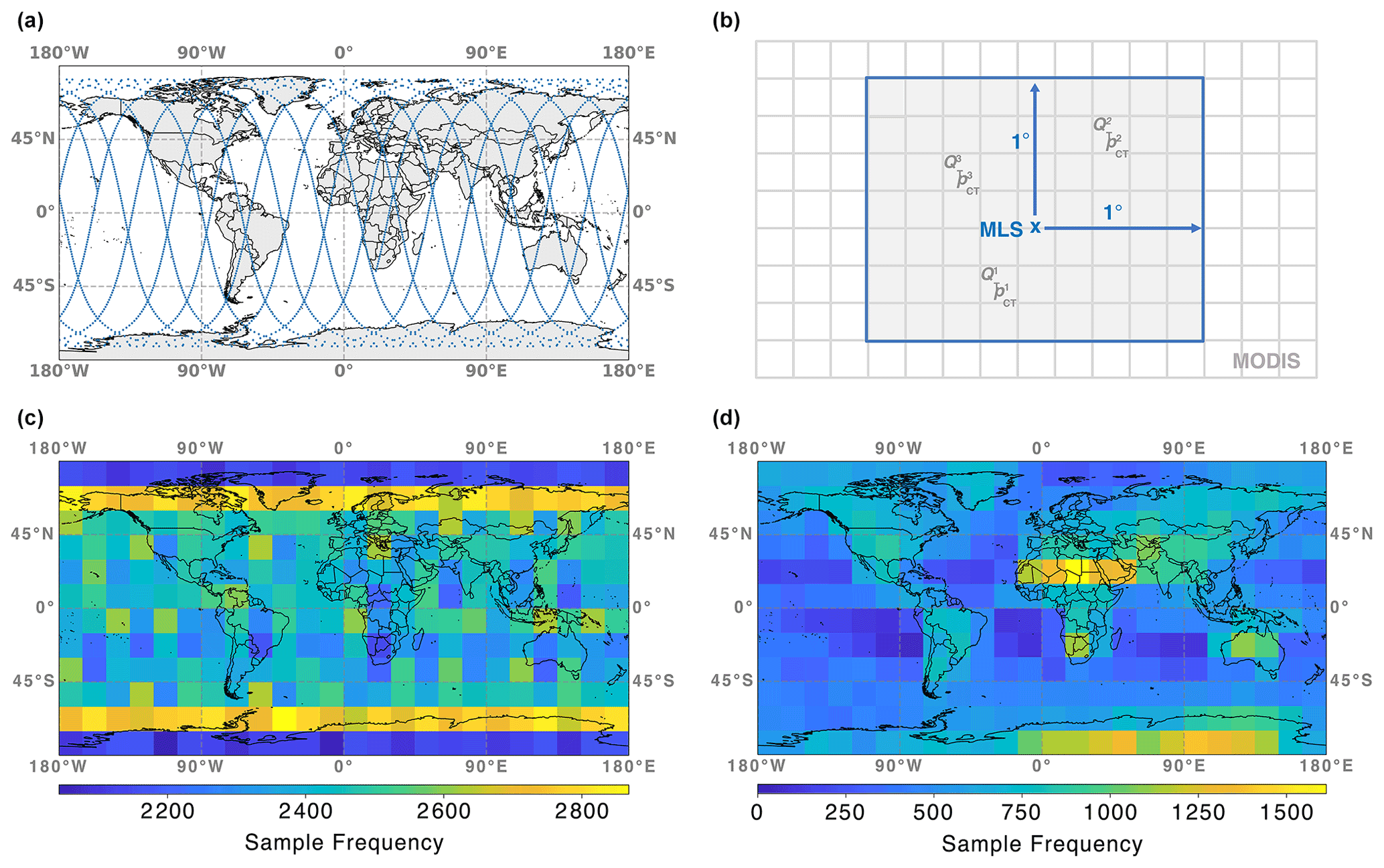
Figure 2(a) Example MLS orbit on 19 May 2019. (b) Illustration of the colocation of MLS and MODIS data. (c) Global map of sample frequencies for the colocated MLS–MODIS data set used in this study. (d) Same as (c) but showing the sample frequencies of observed clear and cloudy profiles, following the definitions in Sect. 3.2.
3.2 The labels from colocated MLS–MODIS cloud data
Training data for the output vector L, which contains the prescribed labels for Eq. (8), are provided by the MODIS Collection 6.1 data set described in Sect. 2. The reported MODIS cloud products are first colocated with individual MLS profiles.
An example MLS orbit on 19 May 2019 is shown in Fig. 2a. Each blue dot represents 1 of the ∼ 3500 daily profiles sampled by MLS. Note that there are three latitudinal ranges (in the tropics and Northern and Southern Hemisphere mid-latitudes), where the ascending and descending orbits cross multiple times a day. Since the inclination angle of Aura is close to 90∘, both polar regions contain more MLS profiles than other locations.
The illustration in Fig. 2b depicts how colocation is performed. If nper is the number of MODIS pixels (gray-shaded squares) within a 1∘ × 1∘ box (in latitude and longitude; blue box) around an MLS profile (blue “x”), then each of the nper pixels reports a cloudiness flag, as well as a total water path () and a cloud top pressure (), with denoting the individual pixels within the 1∘ × 1∘ box. Note that for legibility the cloud properties of only three MODIS pixels are shown. For the respective MLS profile, these parameters are aggregated to more general cloud statistics consisting of the cloud cover (C) within the 1∘ × 1∘ box, as well as the median total water path (QT) and median cloud top pressure (pCT). Note that no significant decrease in classification performance is observed for varying aggregation scales between 0.5∘ × 0.5∘ and 2∘ × 2∘.
Figure 2c shows the global distribution of sample frequencies for the colocated MLS–MODIS data set within grid boxes of length 15∘ × 15∘ (latitude and longitude). While not every grid box contains the same number of profiles, each area contains at least 2100 MLS–MODIS samples. A maximum in sample frequency is observed over the regions with denser MLS coverage around the poles.
The aggregated profile-level cloud statistics are used to define the observed clear-sky and cloudy conditions. All profiles that are characterized by , pCT < 700 hPa, and QT > 506 g m−2 are labeled as cloudy, while profiles with and QT < 25 g m−2 are considered to be associated with clear-sky samples. While the cloud cover threshold is somewhat arbitrary, the pCT limit for cloudy observations and the QT thresholds are carefully selected. The large opacity of the atmosphere for longer path lengths means that MLS shows almost no sensitivity towards clouds with pCT≥ 700 hPa (see Sect. 3.3). This upper pressure limit, which in the 1976 U.S. Standard Atmosphere (COESA, 1976) is located at an altitude of ∼ 3 km, is around the lower limit of observed cloud tops of mid-level cloud types (e.g., altostratus and altocumulus). The 10th and 25th percentiles of all profiles containing clouds within the 1∘ perimeter, regardless of C, are QT∼ 25 g m−2 and QT∼ 50 g m−2, respectively. These definitions have an additional benefit: they almost evenly split the data set into cloudy and clear-sky profiles (52.0 % and 48.0 %, respectively), which improves the reliability of the trained weights for the cloud classification.
Naturally, these definitions leave some profiles undefined (e.g., those with C in the range –). These profiles (about the number of the combined cloudy and clear classes) cannot be included in the training of the ANN, as they lack a prescribed label. The discussion in Sect. 4.1 provides an analysis of the ANN performance for a redefined classification based on a simple threshold of C=0.5 (in addition to a positive QT) to distinguish between cloudy and clear-sky profiles.
Figure 2d shows the global distribution of sample frequencies for the training data set, which comprises the clear-sky and cloudy labels defined earlier. Here, the observed patterns depend strongly on the MODIS-observed cloud conditions (see Sect. 4.3 for more information). Regions with comparatively low cloud cover (most of the African continent, as well as Australia and Antarctica) and those with increased occurrences of high and mid-level clouds (mostly over land) show higher sample frequencies compared to areas over the oceans. Three regions with low sample frequencies, west of South America, Africa, and Australia, stand out. Those areas are characterized by increased C of low clouds of up to 80 % (e.g., Muhlbauer et al., 2014). Similar patterns are observed over the North Pacific and Atlantic oceans, albeit to a lesser extent. Those MLS profiles are influenced by clouds that are either too low or exhibit and are therefore not included in the training data set (i.e., are part of the undefined class mentioned earlier).
It is important to note that the difference in viewing geometry between MLS and MODIS (i.e., limb geometry versus nadir viewing) induces a considerable degree of uncertainty in the colocation. While it is reasonable to assume that the majority of a potential cloud signal (or lack thereof) will come from the 1∘ × 1∘ box around the respective MLS profile, there are certain scenarios that will lead to a false classification. The most likely such scenario consists of an MLS line of sight that passes through a high-altitude cloud before a clear-sky 1∘ × 1∘ box. Here, MLS will detect a strong cloud signal, even though the nadir-viewing MODIS instrument does not record any cloudiness at the location of the respective MLS profile. Less likely is the scenario of a very low-altitude cloud located right after (in terms of an MLS line of sight) a clear-sky 1∘ × 1∘ box. This would also result in a false cloud classification (if the MODIS observations are taken as reference). However, because of the increase in atmospheric opacity, the sensitivity of the MLS instrument towards signals further along the line of sight decreases, and it is less likely that MLS would detect these cloud signals in any case. One contributor to the overall uncertainty that is of less concern is the time difference between the Aqua and Aura orbits (∼ 15 min). Because MLS looks forward in the limb, the temporal discrepancy between the sampling of individual MLS profiles and the colocated MODIS pixels is in the range of 0.6–1.4 min. The results presented in Sect. 3.4 illustrate that by training the ANN with a large data set, as well as cross-validating the training results against a large number of random validation data, the contributions of uncertainties associated with colocation (both in space and time) can be considered small and do not overly impact the reliability of the cloud detection algorithm.
The reader is also reminded of the fact that the proposed ANN schemes will try to reproduce, as best as they can, the MODIS-retrieved cloud variables. Those parameters, however, have their own uncertainties and biases, and the ANN will inherently learn those MODIS-specific characteristics. As a result, the ANN predictions should not be considered the true atmospheric state. Instead, they represent a close approximation of the observed values in the colocated MLS–MODIS data set.
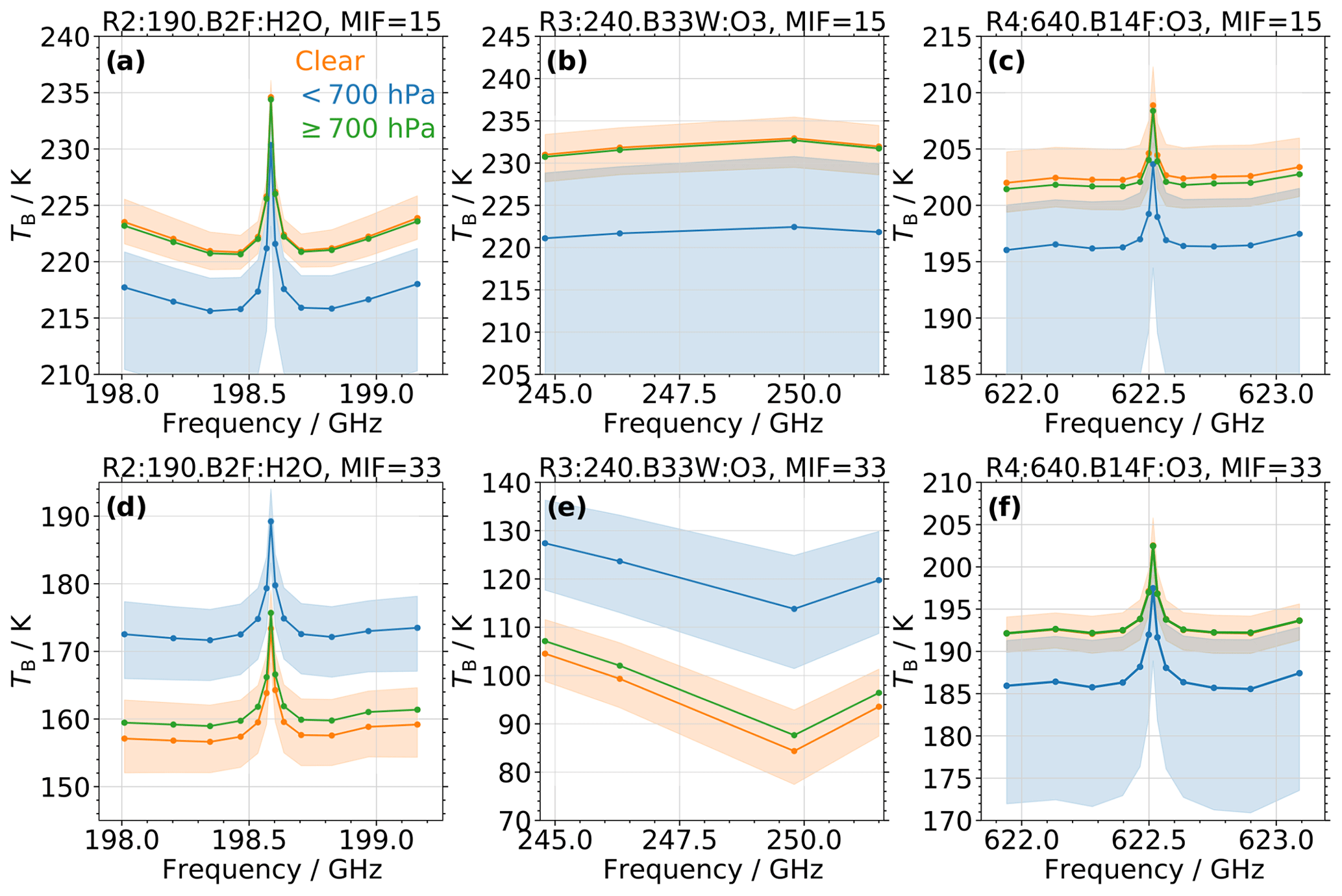
Figure 3(a) Statistic of the brightness temperature (TB) from MLS observations sampled in band 2 of receiver 2 at minor frame (MIF) 15 (at an altitude of ∼ 4.5 km) in the latitudinal range of −30 to +30∘ as a function of frequency. The orange, blue, and green curves show the median TB associated with clear-sky conditions, clouds with a cloud top pressure pCT< 700 hPa, and clouds with pCT≥ 700 hPa, respectively. The orange- and blue-shaded areas indicate the interquartile range of the respective TB (omitted for low clouds to enhance legibility). Samples are provided by the colocated MLS–MODIS data set. (b) Same as (a) but for band 33 of radiometer 3. (c) Same as (a) but for band 14 of radiometer 4. (d–f) Same as (a–c) but at MIF = 33 (at an altitude of ∼ 12 km).
3.3 The input matrix from MLS brightness temperature observations
Figure 3a–c show the spectral behavior of TB sampled in MLS bands 2, 33, and 14 at MIF = 15, which on average corresponds to ptan∼576 hPa (at an altitude of ∼ 4.5 km in the 1976 U.S. Standard Atmosphere). In this section we mostly omit the superscript j to indicate the statistical analysis of all values in the respective band (). The median TB for profiles associated with clear-sky (orange) and cloudy conditions (blue), based on the classifications from the colocated MLS–MODIS data set described in Sect. 3.2, are shown by the solid lines and circles. The orange- and blue-shaded areas indicate the interquartile range (IQR; 75th–25th percentile of data points) of clear and cloudy profiles. Data are from profiles sampled in the latitudinal range of −30 to +30∘.
Median clear-sky profiles exhibit consistently larger TB than cloudy observations, with differences of up to 10 K. This behavior confirms the findings in Wu et al. (2006), where ice clouds at an altitude of 4.7 km reduce band 33 TB at the lower minor frames (i.e., larger ptan). The IQR ranges of the two different data sets are very close for band 2 observations (i.e., within 1–2 K), while there is overlap for the TB sampled in bands 33 and 14.
To illustrate the reduced sensitivity of MLS to signals from very low clouds, the median TB from profiles with pCT≥ 700 hPa is shown in green (for clarity the corresponding IQR is omitted). These profiles behave similarly to clear-sky observations, and the difference in median TB is less than 1 K.
Figure 3d–f illustrate the spectral behavior of TB sampled at MIF = 33, which corresponds to an average ptan of ∼ 200 hPa (at an altitude of ∼ 12 km in the 1976 U.S. Standard Atmosphere). Similar to the results for the lower MIF, a clear separation between median TB from clear-sky and cloudy (100 hPa ≤ pCT < 700 hPa) profiles is observed, while those profiles associated with low clouds (pCT ≥ 700 hPa) again behave similarly to clear samples. For observations from bands 2 and 33, the cloudy profiles show significantly higher TB. Again, this confirms the reported behavior in Wu et al. (2006), who found an increase in band 33 TB for cloudy conditions compared to the clear background. Conversely, band 14 observations behave similarly to those sampled at MIF = 15, and the cloudy profiles exhibit lower TB.
The significant contrast in median TB between clear-sky and cloudy profiles, especially for band 2 and partly for band 33, might suggest the possibility of a simple cloud detection approach via thresholds. However, the respective IQR ranges often overlap, which indicates that a simple TB threshold would miss about 25 % of both the clear and the cloudy data. Moreover, the behavior illustrated in Fig. 3 is specific to the latitudinal range of −30 to +30∘. For higher latitudes, changes in atmospheric temperature and composition yield a noticeable decrease in the observed contrast, while close to the poles the clear-sky profiles almost always have lower TB than the cloudy observations (even at the lower MIFs). A more sophisticated classification approach, with TB samples from additional MLS bands and minor frames, is necessary to derive a more reliable global cloud detection.
Table 1Details of the input variables for the ANN algorithm, which consist of MLS brightness temperature observations in 10 different bands from 4 radiometers. Besides the official radiometer and band designations, the local oscillator (LO) and primary species of interest in the respective band are given, as well as the ranges of minor frames (MIFs) and channels used as input for the ANN.

Table 1 details the MLS bands, as well as their associated channels and MIFs, that comprise the m × n input matrix for the ANN. The input matrix consists of m different , sampled in individual channels (within the respective MLS bands) and MIFs, at n different times. To reduce the computational costs during the training of the model, not all MLS observations are considered. Instead, 10 different bands are chosen in total. Those are bands 2, 3, and 6; 7, 8, and 33; and 10, 14, and 28 for the 190, 240, and 640 GHz spectral regions, respectively. These bands were carefully selected after a statistical analysis of the altitude-dependent contrast in observed TB between clear and cloudy profiles. This contrast is generally low (in the range of 1 K) for the observations from the 118 GHz region, so only band 1 from this receiver is included in the model input. For most of the 10 bands, every second channel is included in the input (except for band 33, which only has four channels in total), while considering every third MIF in the range 7–49 yields decent vertical resolution between 15 hPa (for the highest altitudes) and 150 hPa (at the lowest altitudes). Overall, the input matrix for the training and validation of the ANN is of the shape 1710 × 162 117; i.e., it consists of m = 1710 different features ( at different frequencies and altitudes) from n = 162 117 MAFs (either classified as clear sky or cloudy).
3.4 Training and validation
The Keras Python library provides convenient ways to manage the setup, training, and validation of ANN models. The optimal weights for Eqs. (2)–(6) are derived in four steps: (i) defining an independent test data set which comprises 10 % of the clear and cloudy cases and will be used to evaluate the final model; (ii) determining the most appropriate hyperparameters via k-fold cross validation; (iii) training and validating a number of different models with the best set of hyperparameters on multiple, random splits between training and validation data sets; and (iv) comparing the performance scores for the different model runs to evaluate the stability of the approach and pick the best set of weights.
The hyperparameters to be determined are (i) the number of hidden layers, (ii) the number of neurons per hidden layer, (iii) the optimizer for the cloud classification, (iv) the mini-batch size, (v) the learning rate, and (vi) the value for the weight decay (i.e., the L2 regularization parameter). The number of hidden layers and neurons impact the complexity of the model. The choice of optimizer controls how fast and accurately the minimum of the loss function in Eq. (8) is determined, based on different feature sets and minimization techniques. During each iteration the model computes an error gradient and updates the model weights accordingly. Instead of determining the error gradient from the full training data set, our models only use a random subset of the training data (called a mini-batch) during each iteration. This not only speeds up the training process but also introduces noise in the estimates of the error gradient, which improves generalization of the models. The learning rate controls how quickly the weights are updated along the error gradient. Thus, the size of the learning rate affects the speed of convergence (higher is better) and ability to detect local minima in the loss function (lower is better). Meanwhile, L2 regularization is one method to specify the regularization term R in Eq. (8), where the sum of the squared weights is multiplied with the L2 parameter:
Note that for clarity we omitted the indices for the weights in Eq (9). The amount of regularization is directly proportional to the value of the L2 weight decay parameter. Regularization usually improves generalization of the models. More information about ANN hyperparameters and their impact on the reliability of model predictions can be found in, e.g., Reed and Marks (1999) and Goodfellow et al. (2016).
The optimal number of hidden layers and neurons was determined to be in the range 1–2 and 100–1200 (in increments of 100), respectively. The mini-batch size alternated between 25 and 213. The learning rate was varied between 10−6 and 10−2 in increments of two levels per decade; the L2 parameter covered a range between 10−7 and 10−1 (as well as L2=0).
The number of epochs (i.e., the number of iterations during the training process) is not considered an important hyperparameter for this study. Instead, the models are run with a large number of epochs, and the lowest validation loss is recorded, so an increase in validation loss during the training (i.e., cases where the model is overfitting the training data at some point) has no impact on the overall performance evaluation. Note that the lowest validation loss usually occurred after ∼ 2000–3000 epochs for both the cloud classification and pCT prediction. No obvious increase in validation loss was observed, even for a large number of epochs.
3.4.1 Determining the hyperparameters
At first, the remaining 90 % of data points (after removing the random test data set) are randomly shuffled and split into k=4 parts. Subsequently, one of the four parts is used as the validation data set, and the other three are used to train the ANN with a certain set of hyperparameters. Here, each of the 1710 features is individually standardized, i.e., each input variable is transformed to have a mean value of 0 and unit variance. This step is essential for a successful ANN training, as the individual features are characterized by different dynamic ranges. Meanwhile, the labels for clear and cloudy profiles are simply set to 0 and 1, respectively. For the pCT models the labels are simply set to the respective pCT values. After model convergence and determination of a set of performance scores, the model is discarded and a different set of three parts is used for training (the remaining fourth part is again used for validation). After cycling through each of the four parts (and recording four sets of performance scores), the set of hyperparameters is changed, and the process begins anew. An evaluation of each set of performance scores, for each set of hyperparameters, reveals the appropriate setup for the ANN.
The performance scores employed for the cloud classification training are three commonly used binary classification metrics, based on the calculation of a confusion matrix M for the two classes (i.e, clear-sky and cloudy profiles). If tp and tn are the number of true positives and negatives, respectively, and fp and fn are the number of false positives and negatives, respectively, then the confusion matrix is defined as
From M the accuracy (Ac), F1 score (F1), and Matthews correlation coefficient (Mcc) can be derived as
While Ac quantifies the proportion of correctly classified samples, F1 describes the harmonic mean value between precision (proportion of true positives in the positively predicted ensemble, i.e., the ratio of tp to tp + fp) and recall (proportion of correctly predicted true positives, i.e., the ratio of tp to tp + fn). Generally, F1 assigns more relevance to false predictions and is more suitable for imbalanced classes, where the respective data sizes vary significantly. All elements of the confusion matrix are important in determining the Mcc, which yields values between −1 and 1 and thus is analogous to a correlation coefficient.
The performance evaluation for the pCT prediction application, on the other hand, is based on the Pearson product-moment correlation coefficient (r) and root mean square deviation (RMSD).
For the cloud classification application, this analysis revealed that models using one hidden layer slightly outperformed those with two hidden layers. The number of neurons per hidden layer had a negligible impact, as long as the number was larger than 200. However, the models with 800 and 900 neurons exhibited average Ac values that were 0.0002 higher than those of other setups. We ultimately set it to 856, which corresponds to the average between the number of nodes in the input and output layers (i.e., 1710 and 1, respectively). The Adam optimizer with a learning rate of 10−5 yielded the overall best validation scores for the cloud classification. Note that we applied the Adam optimizer with the standard settings described in the Keras documentation. The best L2 parameter and mini-batch size values were found to be 50−4 and 1024 (i.e., 0.8 % of the training data), respectively. Note that while the choice of L2 had the largest influence on model performance, the impact of the mini-batch size was comparable to the number of neurons (as long as it was >26).
For the pCT prediction, two-layer models noticeably outperformed single-layer ones, as the drop in average r was > 0.01. Again, the number of neurons had only a minimal impact on model performance, with variations in r of ∼ 0.02. However, models with 800–1000 neurons performed best, so we again set this number to 856. The best optimizer, learning rate, L2 parameter, and mini-batch size were found to be Adam, 10−4, 50−4, and 1024, respectively.
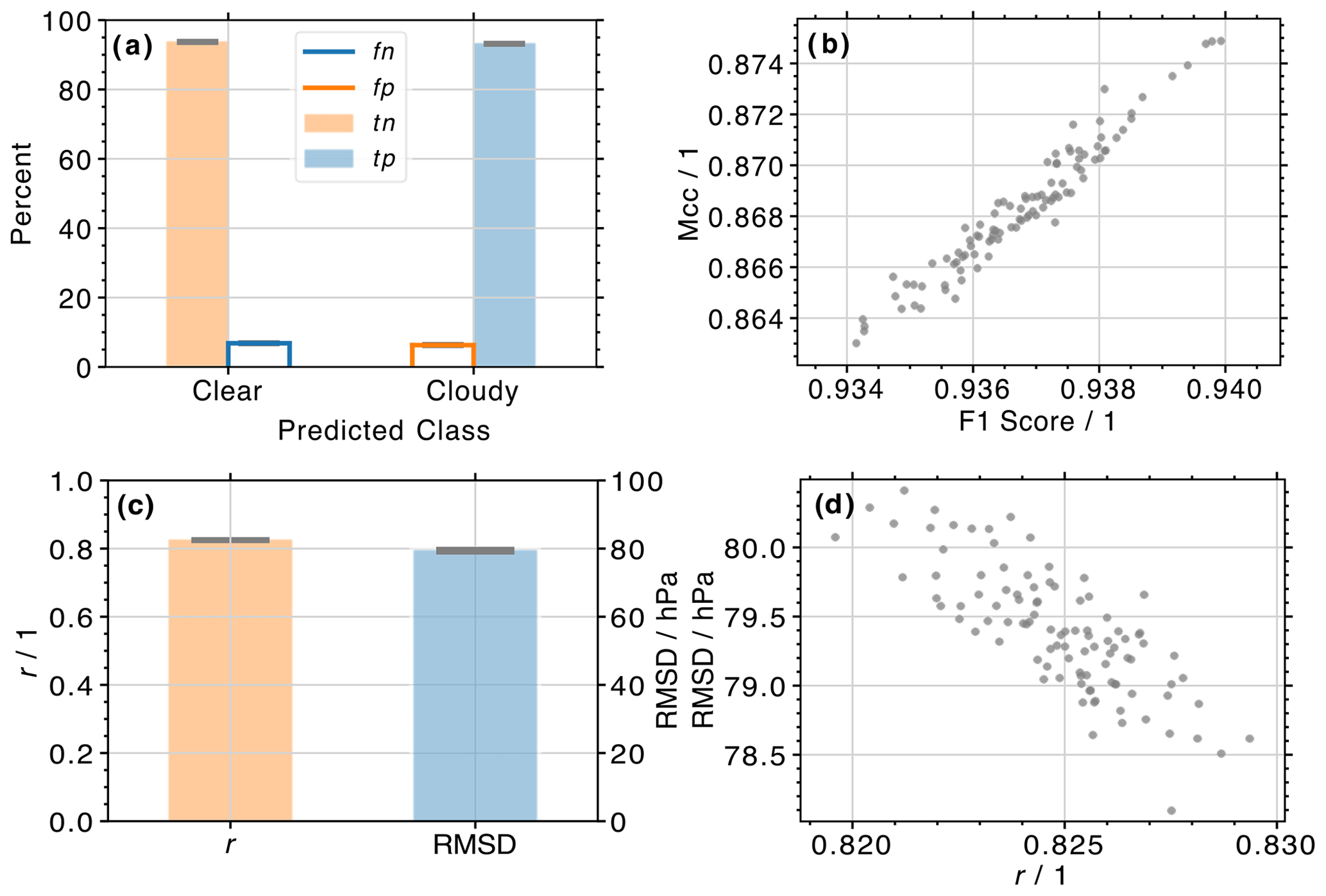
Figure 4(a) Histograms of cloud classifications from the ANN algorithm for 100 random combinations of training and validation data sets. Orange and blue shading depicts the percent of correctly predicted clear (i.e., true negatives, tn) and cloudy (i.e., true positives, tp) labels for actually observed clear and cloudy profiles, respectively. Orange and blue lines depict the percent of falsely predicted cloudy (i.e., false positives, fp) and clear (i.e., false negatives, fn) labels for actually observed clear and cloudy profiles, respectively. The vertical extent of the gray horizontal bars on top of each histogram indicates the standard deviation derived from all 100 predictions (the horizontal extent is arbitrary). (b) Scatter plot of Matthews correlation coefficient (Mcc) and F1 score for the same 100 random combinations of training and validation data sets shown in (a). (c) Similar to (a) but showing histograms of derived Pearson product-moment correlation coefficient (r) and root mean square deviation (RMSD) from the ANN cloud top pressure algorithm. (d) Similar to (b) but showing the relationship between r and RMSD.
3.4.2 Validation statistics
Due to randomness during the assignment of individual observations to either the training or validation data set, developing a single model might result in evaluation scores that are overly optimistic or pessimistic. By chance, the most obvious cloud cases (e.g., C=1 and very large QT values) might have ended up in the validation data set or vice versa, and the trained weights might be inappropriate. Moreover, a large disparity in validation scores for multiple models might be indicative of an ill-posed problem, where the MLS observations do not provide a reasonable answer to the cloud classification problem. Therefore, developing multiple models with a reasonable split of training and validation data, as well as careful monitoring of the spread in validation scores, is imperative. In this study, 100 different models are developed. Before each model run, the data set (minus the test data set) is randomly shuffled and split into training and validation data. The splits between training, validation, and test data are set to 70 %, 20 %, and 10 %. The hyperparameters are identical for each model. As mentioned earlier, each model is run with a large number of epochs, and the weights associated with the lowest validation loss are recorded. Training of these 100 models took ∼ 1 d.
The output of each cloud classification model is a cloudiness probability (P) between 0 (clear) and 1 (cloudy). Note that throughout this study we simply group each prediction in either the clear or cloudy class; i.e., MAFs with predicted probabilities 0≤P < 0.5 are considered to be sampled under clear-sky conditions, while MAFs with are considered to be cloudy. The one exception is the discussion in Sect. 4.2, where the actually predicted P values are employed to study the ANN performance for undefined cloud conditions (with respect to the clear-sky and cloudy definitions presented in Sect. 3.2).
A summary of the derived prediction statistics is shown in Fig. 4a. Each histogram shows the average percentage of correctly predicted clear-sky (i.e., tn, orange shading) and cloudy (i.e., tp, blue shading) labels for all 100 validation data sets. Also shown are the percentages of false classifications (the blue and orange lines for fn and fp, respectively). The gray-shaded horizontal areas at the top of each histogram illustrate the standard deviation for each class, calculated from the 100 validation data sets. The average percentage of correct clear-sky and cloudy predictions is 93.7 % and 93.2 %, respectively, while a false cloudy or clear-sky prediction occurs for 6.3 % and 6.8 % of profiles in the validation data. The standard deviation for all four groups is 0.2 %.
Figure 4b shows a scatter plot of all Mcc values as a function of F1. Even though the Mcc penalizes false classifications more severely than F1, a high r of 0.97 is observed. Moreover, there is little variability in the 100 derived binary statistical metrics, with average Ac, F1, and Mcc values of 0.934 ± 0.001, 0.937 ± 0.001, and 0.868 ± 0.003. These results illustrate that the derived models are well suited to predict cloudiness for new MLS data (i.e., measurements not involved in the training of the models) and that the trained weights are very stable (i.e., all models exhibit very similar binary statistics, regardless of the respective training or validation data set).
Similarly, histograms of r and RMSD (referring to the relationship between the predicted and MODIS results for the validation data), as well as the regression between the two variables, are shown in Fig. 4c and d, respectively. Average values of 0.819 ± 0.001 (r) and 80.268 ± 0.160 hPa (RMSD) are observed. The correlation between the two parameters is r = −0.77.
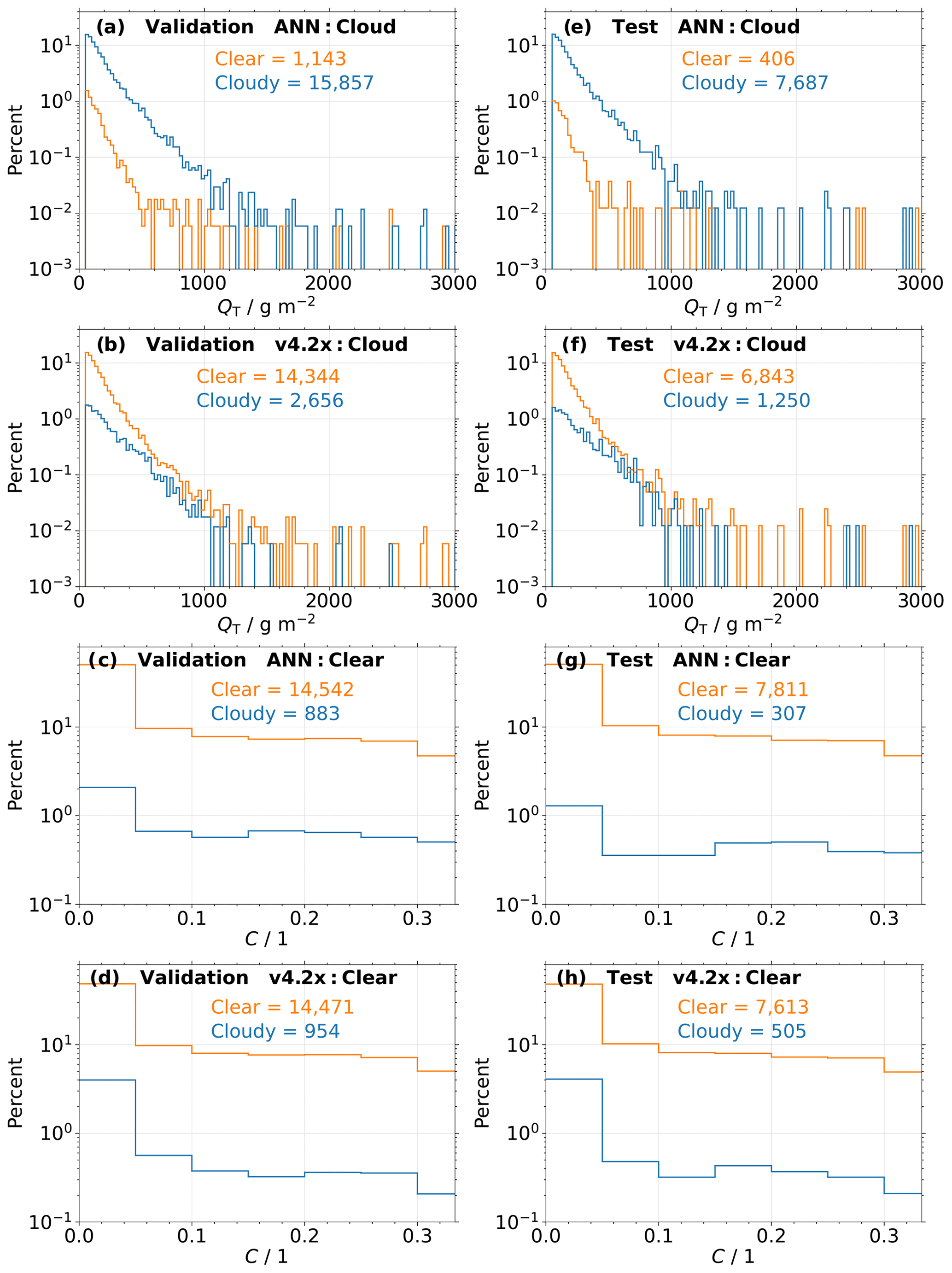
Figure 5(a) Histograms of cloud classifications from the new ANN-based cloud flag for actually observed cloudy profiles as a function of total water path (QT). Only profiles from the validation data set are considered. Orange and blue colors depict the distributions of predicted clear and cloudy labels, respectively. The number of clear and cloudy predictions is also given. (b) Same as (a) but for classifications from the current v4.2x cloud flag. (c, d) Similar to (a, b) but for actually observed clear profiles as a function of cloud cover (C). (e–h) Same as (a–d) but for profiles from the test data set.
Given the statistical robustness of the results, the model with the highest Mcc and lowest RMSD provides the ANN weights for cloud classification and pCT prediction in this study, respectively.
This section includes a detailed comparison between the predicted cloud classifications from the current MLS v4.2x and the new ANN-based algorithms in Sect. 4.1, followed in Sect. 4.2 by a discussion of predicted cloudiness probabilities that illustrates the performance of the new ANN cloud flag for less confident cases (i.e., those outside of the training, validation, and test data sets). This section also presents an analysis of the latitudinal dependence of the ANN performance and derived global cloud cover statistics in Sect. 4.3, as well as a close-up look at cloudiness predictions for some example scenes over both the North American and Asian monsoon regions (Sect. 4.4).
Table 2Binary classification statistics for the new ANN algorithm, as well as the classification provided by the current MLS v4.2x status flag. Prescribed labels (i.e., clear sky or cloudy) are provided by the standard definitions presented in Sect. 3.2; statistics are given for both the validation and test data sets. Results for two modified definitions based on looser thresholds are also given; here statistics are based on all profiles in the MLS–MODIS data set (minus the training data). The fraction of true positives and negatives (tp and tn), as well as false positives and negatives (fp and fn), is given. Finally, three measures for the evaluation of binary statistics are listed: the accuracy (Ac), the F1 score (F1), and the Matthews correlation coefficient (Mcc).

Note that a comparison between v4.2x and ANN results will naturally favor the ANN predictions, particularly any comparison made with reference to MODIS observations. Evaluating the performance of each cloud flag is based on the respective agreement to the MODIS-observed cloud conditions. However, the ANN is designed to replicate the MODIS results, while the v4.2x algorithm is not aware of the MODIS data set (including its uncertainties and biases).
4.1 Prediction performance of current L2GP and the new ANN cloud flag
The analysis in Sect. 3.4 indicates that the ANN setup can reliably reproduce the cloudiness conditions identified by the colocated MLS–MODIS data set. Figure 5 provides a closer look at the performance of the new ANN-based and v4.2x cloud flags for all n = 32 425 (16 211) profiles associated with either the clear-sky or cloudy class in the validation (test) data set.
Figure 5a and b present the percentage of correctly classified (blue) and falsely classified (orange) cloudy validation profiles, as determined by the cloudiness definition for the colocated MLS–MODIS data set described in Sect. 3.2. The frequency of predicted labels from the (a) new ANN-based algorithm and (b) v4.2x cloud flag are shown as a function of QT. Note that because of the general cloudiness definition, only those profiles with QT > 50 g m−2 are considered (see Sect. 3.2). The flags predicted by the ANN correctly classify 93.3 % of the cloudy profiles. In particular, the thickest clouds, those with QT≥ 1000 g m−2, are detected in 78.0 % of cases. Conversely, the current v4.2x status flag only detects 15.6 % of the cloudy profiles. A peak of 15.4 % of clouds is missed for low QT, where the ANN performs significantly better. This is understandable, as the current v4.2x status flags for high and low cloud influences should only be set for profiles where the extinction along the line of sight is large enough to be attributed to a fairly thick cloud. However, even for very large QT≥ 1000 g m−2, only 25.8 % of the cloudy profiles are detected.
Histograms for clear-sky observations in the validation data set as a function of C are presented in Fig. 5c and d. Only 5.7 % of clear profiles are falsely classified as cloudy by the new ANN algorithm, while the current v4.2x status flag mislabels 6.2 % of these profiles. Most of the clear observations occur for very low values of C of <0.05, of which the ANN and v4.2x flags detect 50.4 % and 48.5 %, respectively. Note that the slightly larger fraction of false positives from the v4.2x flag is not necessarily incorrect; i.e., there might actually be clouds in the line of sight of one or more MLS scans associated with the respective profiles. They might, however, be well before (very high clouds) or past (very low clouds) the tangent point and outside of the 1∘ × 1∘ box defined in Sect. 3.2.
Similar histograms for the test data set are shown in Fig. 5e–h. The ANN correctly identifies 95.0 % and 96.2 % of the cloudy and clear cases, respectively, as well as 76.6 % of the QT≥ 1000 g m−2 and 51.0 % of the C<0.05 profiles. The respective fractions detected by the current v4.2x status flag are 15.4 %, 93.8 %, 26.6 %, and 48.2 %.
Table 2 gives an overview of the confusion matrix elements for each cloud flagging scheme, as well as metrics to evaluate binary statistics. For the validation data the new ANN algorithm yields values of Ac = 0.94, F1 = 0.94, and Mcc = 0.87 (Ac = 0.96, F1 = 0.96, and Mcc = 0.91 for the test data), confirming the reliable classification performance shown in Fig. 5. The v4.2x flag yields low binary performance scores of Ac = 0.53, F1 = 0.26, and Mcc = 0.15 for the validation data (Ac = 0.55, F1 = 0.25, and Mcc = 0.15 for the test data), mainly due to the low fraction of true positives.
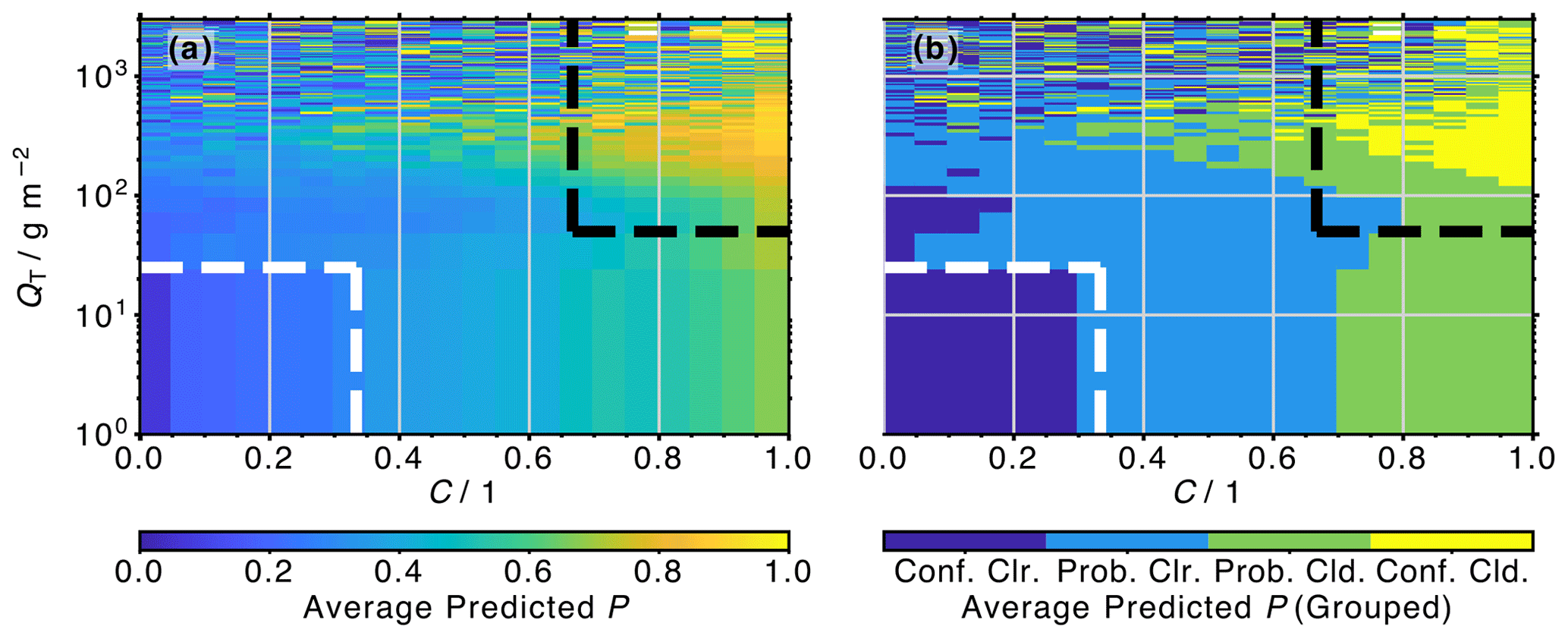
Figure 6(a) Average probability of cloudiness (P) predicted by the ANN as a function of C and QT. No restrictions on cloud top pressure (pCT) are imposed. (b) Same as (a), but P is grouped into four classes: confidently clear (“Conf. Clr.”; P<0.25), probably clear (“Prob. Clr.”; ), probably cloudy (“Prob. Cld.”; ), and confidently cloudy (“Conf. Cld.”; P≥0.75).
4.2 Probabilities for different cloud conditions
The clear-sky and cloudy classes defined in Sect. 3.2 leave a number of profiles unaccounted for (i.e., neither clear sky nor cloudy), such as those with ≤C < or pCT≥ 700 hPa. While it is reasonable to only train the model on the confidently clear and cloudy conditions, it is essential to understand the ANN performance for the undefined, in-between cases.
Figure 6a shows average ANN-predicted cloudiness probabilities as a function of C and QT with no restrictions on pCT. Data that the ANN were trained on are excluded from this analysis. Figure 6b illustrates the distribution when P values are distributed into four groups: confidently clear (Conf. Clr.; P < 0.25), probably clear (Prob. Clr.; 0.25 ≤P < 0.5), probably cloudy (Prob. Cld.; 0.5 ≤P < 0.75), and confidently cloudy (Conf. Cld.; P≥ 0.75). The previously defined clear-sky and cloudy regions are indicated by the white and black dashed lines, respectively. Profiles with low values of and QT < 25 g m−2, regardless of pCT, are characterized by the lowest P values, reliably reproducing the clear-sky class defined in Sect. 3.2. Meanwhile, almost all profiles with C>0.7 are flagged to be probably cloudy (P>0.5). However, only profiles that also have QT > 100 g m−2 are reliably predicted to have P>0.75. The less-confident identification of the QT > 100 g m−2 cases reflects the fact that many of them have low cloud tops, pCT≥ 700 hPa, and are thus not readily observed by MLS. As noted in Sect. 3.3, these profiles exhibit similar spectral behavior to clear ones, and the ANN is expected to miss most of these clouds. With increasing QT, even profiles with smaller cloud fractions (as little as C=0.25) are flagged as cloudy. Note that the P results become noisy for very large QT values of > 500 g m−2, conditions that are only observed for less than 4 % of the total samples (< 1 % for QT > 1000 g m−2).
In order to evaluate the ANN performance when more of these uncertain cases are encompassed, we included in Table 2 a comparison of the binary performance scores for a redefined set of the cases classified as clear and cloudy according to less conservative thresholds for the cloud cover and the total water path (C<0.5 and QT < 25 g m−2 for clear-sky profiles and C≥0.5 and QT≥ 25 g m−2 for cloudy profiles). No limitations on pCT are imposed. These changes increase the number of profiles from n = 48 636 (validation and test data) to n = 214 805 profiles. Again, samples from the training data set are excluded. Due to the looser definitions, there is a significant drop in performance scores, which can mostly be attributed to a lower true positive rate (i.e., cloud detection) of 0.58 and 0.05 for the ANN classification and v4.2x, respectively. The fraction of false positives (i.e., false prediction of cloudiness for actually clear profiles) remains basically unchanged (changes of ∼ +0.04 and −0.01 for the ANN and v4.2x flags, respectively). This means that even with a looser cloudiness definition, the ANN does not yield a multitude of false cloud classifications; rather, the algorithm fails to detect a larger fraction of cloudy profiles. As a consequence of the reduced true positive rates for the modified class definitions, the derived F1 for the ANN score is reduced to 0.58 (from ∼0.94), while F1 for the current v4.2x flag drops from ∼0.26 to 0.09. This is almost exclusively due to an inability to detect lower clouds. As demonstrated in Sect. 3.3, MLS cannot distinguish between clear-sky and cloud signals if pCT≥ 700 hPa. Adding a threshold of pCT<700 hPa to the loosened definitions, the performance for the now n = 89 697 profiles is much closer to the one from the validation and test data set. Here, the ANN and v4.2x classifications exhibit Ac=0.90, F1=0.90, and Mcc=0.81 and Ac=0.54, F1=0.22, and Mcc=0.13, respectively.
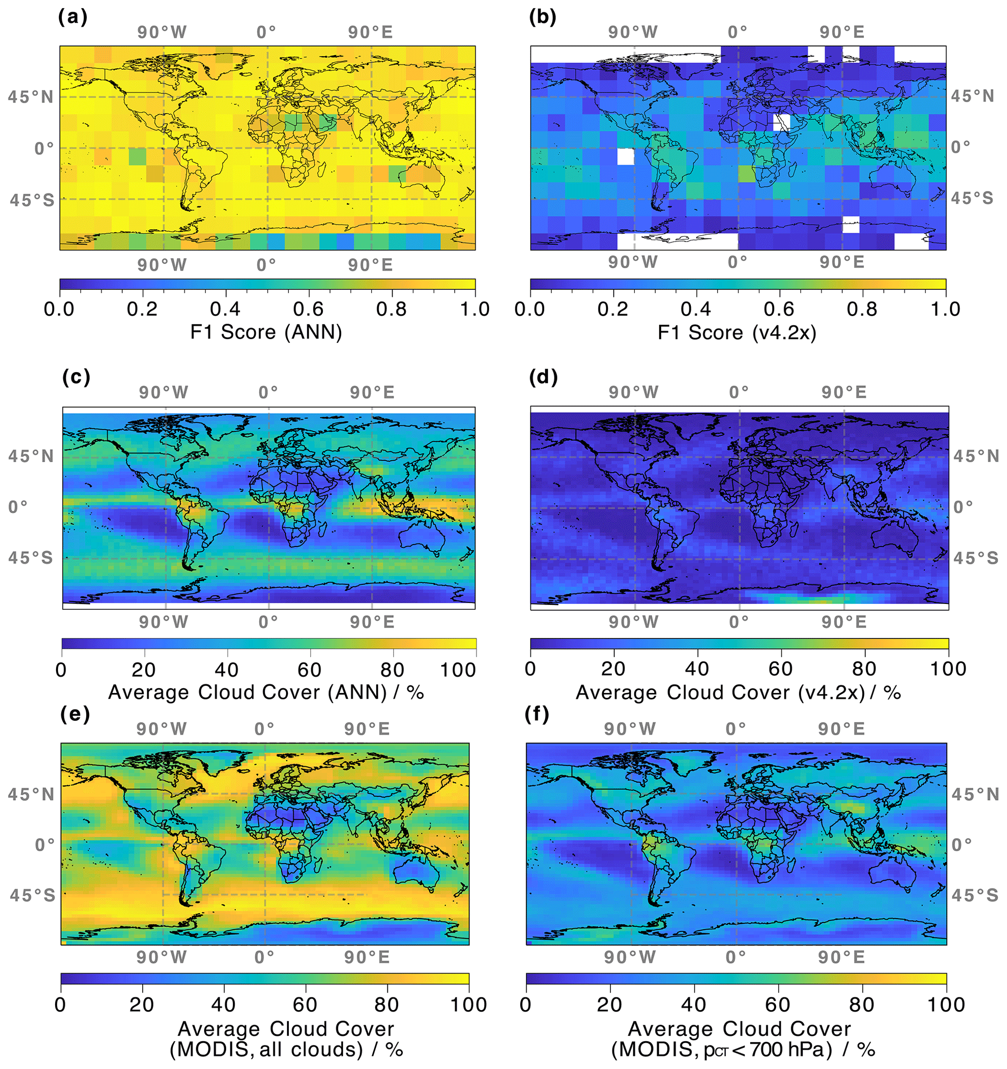
Figure 7(a) Latitudinal and longitudinal dependence of the performance of the ANN algorithm, determined by the F1 score for binary classifications. Observations and actual cloudiness flags are provided by the colocated MLS–MODIS data set; only profiles from the validation and training data set are considered. (b) Same as (a) but for the current v4.2x cloud flag. (c) Average global cloud cover derived from MLS brightness temperature observations and the weights determined from the trained ANN. All MLS observations sampled between 2015 and 2019 are represented. (d) Same as (c) but for the current v4.2x cloud flag. (e) Same as (c) but from Aqua MODIS observations sampled in 2019. (f) Same as (e) but with retrieved cloud top pressure < 700 hPa.
4.3 Geolocation-dependent performance and global cloud cover distribution
The spectral behavior for clear-sky and cloudy profiles shown in Fig. 3 only applies for observations made in the latitudinal range of −30 to +30∘. As mentioned in Sect. 3.3, the contrast between the two classes of data decreases for increasing latitude. While the analysis in Sect. 4.1 illustrates that the new ANN-based cloud classification can reliably identify cloudy profiles (based on the definitions in Sect. 3.2), it is important to make sure that there is no latitudinal bias in the predictions, i.e., assuring that the algorithm performance is good for MLS observations at all latitude bands.
Calculated F1 determined from the ANN model setup is shown in Fig. 7a for different regions of the globe. Statistics are calculated in grid boxes that cover an area of 15∘ × 15∘ (latitude and longitude) and include on average 168 profiles. High values of F1>0.85 are observed for most regions; however, areas with generally low cloud cover (over Africa and Antarctica, as well as west of South America and Australia; see Fig. 7e) exhibit slightly lower classification performance, indicated by the light-blue and green colors. Here, reduced sample statistics yield a less reliable F1 metric, as the number of profiles per grid box is as low as 18. Further analysis shows that the reduced F1 scores within these grid boxes are exclusively due to an increase in false negatives; i.e., the model misses some cloudy profiles. Overall, the average observed F1 is 0.91 ± 0.11.
In contrast to the results for the ANN algorithm, there is a more noticeable latitudinal dependence for the performance of the current v4.2x algorithm illustrated in Fig. 7b. F1 values can be as high as 0.67 in the tropics and < 0.25 everywhere else. Occasional gaps, especially over the polar regions, are due to a failed F1 calculation. Here, the denominator in Eq. (12) becomes 0; i.e., the v4.2x flag only reports clear-sky classifications. The average observed F1 is 0.23 ± 0.16.
As the prediction performance is high for a majority of geographical regions, the ANN algorithm is applied to derive global cloud cover maps, based solely on the MLS observed TB and the calculated model weights. A map of cloudiness from all MLS profiles sampled over 2015–2019, averaged within 3∘ × 5∘ (latitude and longitude) grid boxes, is shown in Fig. 7c. Note that this data set includes more than 6 million MLS profiles, while only 65 d in the 5-year span were part of the training data. Profiles are considered to be cloudy when predicted P≥0.5. Three large-scale regions close to the Equator show the largest average cloud covers with C> 80 % (dark-orange colors): (i) an area over the northern part of South America, (ii) central Africa, and (iii) a large band encompassing the Maritime Continent. Large zonal bands of C∼ 60 % are observed in the mid-latitudes of both hemispheres. Conversely, large areas of low C of <20 % are observed west of the North American, South American, and African continents, as well as over Australia, northern Africa, and Antarctica. The derived cloud covers, as well as the observed spatial patterns of mid to high clouds, agree well with those reported in King et al. (2013) and Lacagnina and Selten (2014).
As before, we are interested in comparing the results of the new ANN classification to the ones from the current v4.2x cloud flag. Therefore, a similar map of derived global cloud cover from the current v4.2x cloud flag is shown in Fig. 7d. In contrast to the ANN results, v4.2x suggests C< 32 % almost everywhere. This behavior is consistent with the focus of the v4.2x classification, where only very opaque clouds around ∼ 300 hPa are flagged. The global patterns identified by the new ANN flag are reproduced, albeit with much lower results for C. However, the v4.2x flag yields a global maximum of C>72 % over Antarctica. Here, the new ANN flag reports C as low as 3 %. This behavior in the v4.2x cloud flag is a well-understood feature caused by misinterpretation of radiances that are reflected by the surface (William Read, personal communications, 2021). Here, the unique combination of high topography and low optical depth makes Antarctica one of the few places where MLS can observe the Earth's surface.
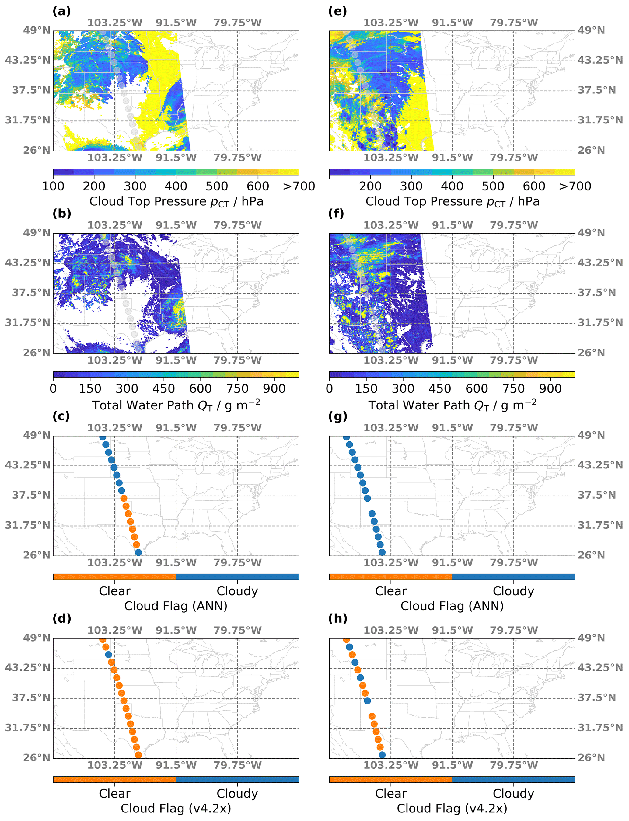
Figure 8(a) Map of cloud top pressure (pCT) retrieved from MODIS observations on 31 August 2017 over North America. Transparent circles indicate the MLS orbit. (b) Similar to (a) but for the total water path (Qt). (c) Clear (orange) and cloudy (blue) profiles as determined from the new ANN algorithm. (d) Same as (c) but determined from the current v4.2x status flags. (e–h) Same as (a–d) but for MLS and MODIS observations on 5 July 2015.

Figure 9Similar to Fig. 8 but for MLS and MODIS observations on (a–d) 28 June 2019 and (e–h) 5 July 2018, respectively, over South Asia. These scenes were captured over the Asian summer monsoon region.
Figure 7e and f show similar cloud cover maps generated from Aqua MODIS observations. Due to the size of that data set and the high computational costs, only samples from 2019 are included here. The cloud cover maps were generated considering cloud mask flag values of 0 and 1 (confident cloudy and probably cloudy) as defined in Menzel et al. (2008). All available 1 km resolution MODIS cloud mask data were considered. The aggregation used the high-resolution cloud top pressure product, not generally available as a global aggregation. This cloud top pressure product, however, is the one utilized by retrievals of MODIS cloud optical properties. Such custom aggregation thus ensures the maximum data set consistency across variables. While all clouds are considered in the map in panel e, only clouds with pCT< 700 hPa are included to derive C in panel f. It is obvious that including clouds with pCT≥ 700 hPa dramatically increases the derived cloud covers. Due to the reduced sensitivity towards such clouds (see the discussion in Sect. 3.3), the cloud covers predicted by the ANN are much closer to the MODIS results that do not include low clouds. Nonetheless, the ANN-derived C values are, on average, ∼ 9 % higher than the MODIS results, suggesting that MLS is able to detect some of the lower clouds with pCT≥ 700 hPa. This behavior is also illustrated in the example scenes in Figs. 8 and 9 in Sect. 4.4. In comparison, there is much poorer agreement between the MODIS and v4.2x results, with v4.2x on average ∼26 % lower than MODIS.
This analysis indicates that the new ANN algorithm can produce considerably more reliable cloud classifications than the v4.2x MLS cloud flag, on a global scale.
4.4 Example scenes
The analysis in the previous sections centered on statistical metrics and the reproduction of large-scale, global cloud patterns. There, the cloud flag based on the new ANN algorithm yields reliable results, both in comparison to the current v4.2x status flag and as a standalone product. However, a more qualitative assessment of the model performance for individual cloud scenes provides additional confidence in the technique, as well as insights into the classification performance for different cloud types. Again, profiles are flagged as cloudy when P≥0.5.
Figure 8 shows two example cloud fields over the North American monsoon region. During the summer months of July and August, this area is characterized by the regular occurrence of mesoscale convective systems that can occasionally overshoot into the lowermost stratosphere, where the sublimation of ice particles can lead to local humidity enhancements (Anderson et al., 2012; Schwartz et al., 2013; Werner et al., 2020). Observed pCT and QT derived from Aqua MODIS observations over the first example scene, sampled on 31 August 2017, are shown in Fig. 8a and b, respectively. The MLS overpass is illustrated in gray transparent circles. A cloud system with pCT< 500 hPa exists in the northern part of the scene, with the lowest pCT at ∼ 200 hPa. The MLS track passes some smaller cloud clusters characterized by large QT, which are indicated in yellow. In the south, low clouds with QT = 50–450 g m−2 are observed. The new ANN and current v4.2x cloud flags are shown in Fig. 8c and d. The ANN algorithm flags every profile in the northern part of the scene as cloudy, while also detecting the very low clouds in the south. Conversely, the classifications from the current v4.2x flag identify a cloud influence for a single MLS profile in the north, which happens to actually be over an area with low QT. A second example cloud field is shown in Fig. 8e–h. This scene consists of clouds all along the MLS track and large areas with elevated QT up to 1000 g m−2. Note that there is a gap in the MLS track, where the Level 2 products are screened out, according to the rules in the MLS quality document (Livesey et al., 2020). The ANN algorithm correctly determines that every profile along the path was sampled under cloudy conditions. However, even for the very high clouds that contain large water abundances, the v4.2x algorithm only occasionally flags the respective profiles as cloudy. In the northern part of the track, the flag actually alternates between clear-sky and cloudy classifications.
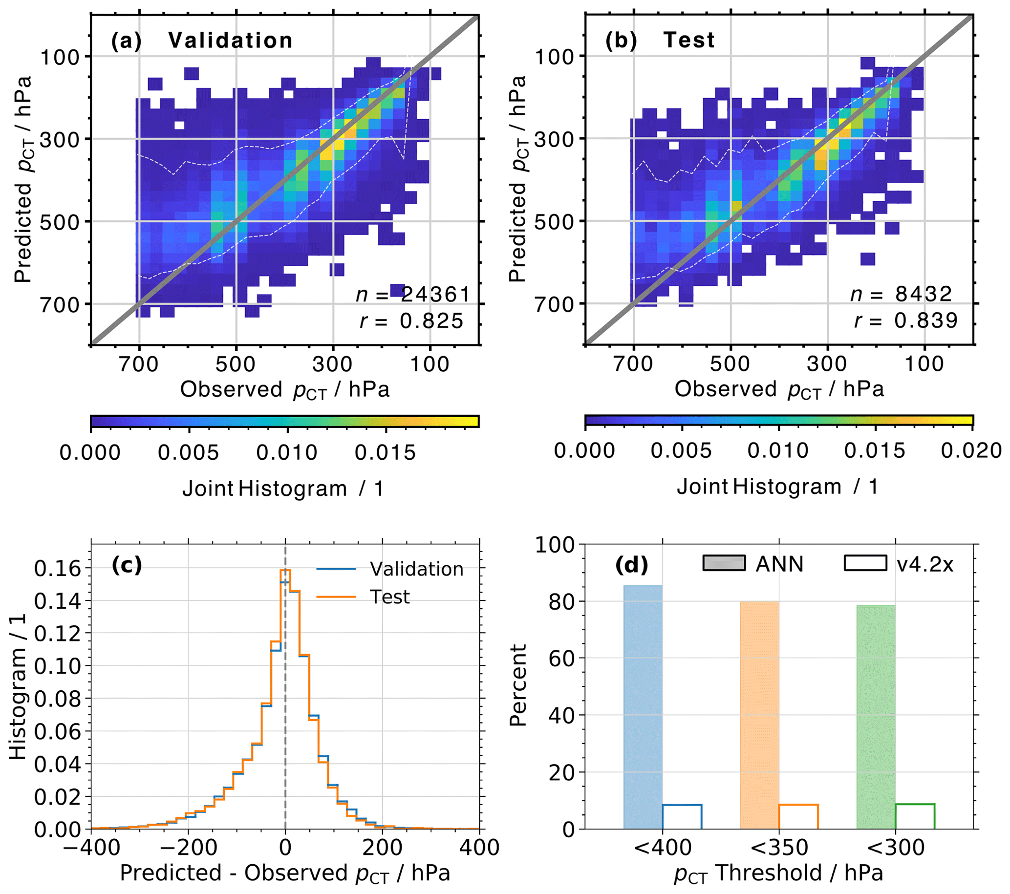
Figure 10(a) Normalized joint histograms of true and predicted cloud top pressure (pCT). Data are from the validation data set. (b) Same as (a) but for the training data set. (c) Histograms of the difference between predicted and observed pCT, for profiles in the validation (blue) and test (orange) data set. (d) Percent of observed pCT < 400, 350, and 300 hPa that was successfully detected by the ANN (color-filled bars) and flagged by the v4.2x algorithm (transparent bars). Data are from both the validation and test data sets.
Similarly, Fig. 9 shows two example cloud fields over the Asian summer monsoon region, which also regularly contains overshooting convection from mesoscale cloud systems. The first scene, shown in Fig. 9a–d, displays a mix of different cloud conditions. There are high clouds with pCT< 350 hPa and QT = 50–450 g m−2 in the northern part, a large clear-sky area in the middle, and then a mix of very high and low clouds in the south that exhibits low QT and likely represents a multilayer cloud structure with thin cirrus above boundary layer clouds. The new ANN-based flag successfully detects both the northern and southern cloud fields, while the current v4.2x flag only detects a single profile with cloud influence. The last example scene, illustrated in Fig. 9e–h, similarly displays a mix of low, mid-level, and high clouds. As expected, the current v4.2x algorithm only flags a single profile as influenced by high clouds (in the south of the scene). However, the ANN algorithm detects the mid-level clouds in the north, as well as the mix of cloud types in the south of the scene. In those places where MODIS mostly captured either low boundary layer clouds (yellow colors) or the cloud property retrieval failed (very low QT), the ANN associates the respective profiles with the clear-sky class.
Note that the two example scenes in Fig. 9 represent previously unseen data for the ANN; i.e., the models were not trained on these MLS–MODIS observations.
The results in Sect. 4 illustrate that the proposed ANN algorithm can successfully detect the subtle cloud signatures in the spectral TB profiles shown in Fig. 3. For many MLS bands, the differences between cloudy and clear-sky TB are usually in the range of just a few Kelvin, and the spectral behavior heavily depends on the respective MIF (i.e., pressure level at the tangent point of each scan). This section demonstrates how this behavior can be used in a similar ANN setup to infer the MODIS-retrieved pCT. Here, our goal is to reliably differentiate between mid-level to low clouds and high-reaching convection with pCT ⪅ 350 hPa. As mentioned in the Introduction, not only can these high clouds impact the MLS retrieval of atmospheric constituents, but they can also breach the tropopause and inject ice particles into the lowermost stratosphere.
This section presents a statistical performance evaluation of the pCT prediction in Sect. 5.1, a global analysis of pCT distributions in Sect. 5.2, and a close-up look at pCT predictions for the same example scenes over the North American and Asian monsoon regions that were shown earlier (Sect. 5.3).
Similar to the cloud classification analysis, a comparison between v4.2x and ANN prediction performance will favor the ANN results, since the ANN is designed to replicate the MODIS observations.
5.1 Performance evaluation
Joint histograms of observed and predicted pCT for all cloudy profiles in the validation and test data set are presented in Fig. 10a and b, respectively. While there is a fair amount of scatter, the majority of data points are close to the 1:1 line. This is illustrated by the envelope indicated by the white dashed line, which is defined by the 5th and 95th percentiles of predicted pCT for each observed pCT bin (i.e., the envelope indicates where 90 % of predicted pCT values are). High values of r=0.825 and r=0.839, with RMSD values of 79.2 and 76.9 hPa, are observed for the two data sets. However, a decline in ANN performance is noticeable for observed pCT> 400 hPa, where predictions for pCT> 600 hPa exhibit an average underestimation of 126 hPa (19.2 %). This is consistent with the findings presented in Sect. 3.3, which showed a reduced sensitivity of MLS observations to low clouds. Conversely, the average difference between predictions and observations is +25 hPa (9.5 %) for MODIS-retrieved pCT< 400 hPa.
Histograms of the difference between predicted and observed pCT for profiles in the validation and test data sets are shown in Fig. 10c. The two distributions look almost identical and are centered around a difference of −8 and −10 hPa, respectively. For the validation data set, 65.6 % (88.0 %) of predictions are within 50 hPa (100 hPa) of the MODIS observations, while 66.9 % and 88.0 % of profiles in the test data set are within these ranges.
As mentioned in the Introduction, we are mostly interested in the ability to detect high clouds with pCT< 400 hPa. Not only can these clouds affect the MLS radiances and retrievals, they can also impact water vapor (e.g., Werner et al., 2020; Tinney and Homeyer, 2020) and HNO3 (e.g., Wurzler et al., 1995; Krämer et al., 2006) concentrations in the upper troposphere and lower stratosphere. Figure 10d shows the percent of profiles in the combined validation and test data set, where the ANN correctly reproduces the MODIS-observed cloud top pressure for thresholds of pCT< 400, 350, and 300 hPa. To provide a comparison to the current v4.2x algorithm performance, we simply calculated the percent of successful cloud detection for each of these pCT thresholds. The ANN correctly identifies 85.4 %, 80.0 %, and 78.5 % of the profiles with pCT< 400, 350, and 300 hPa, respectively. In contrast, the v4.2x flag only detects 8.5 %, 8.6 %, and 8.7 % of these profiles.
The analysis in this section reveals that the ANN setup can predict the MODIS-retrieved pCT with reasonable accuracy, which provides the ability to reliably identify high clouds with pCT<400 hPa.

Figure 11(a) Map of derived Pearson product-moment correlation coefficient (r) between MODIS-retrieved and ANN-predicted cloud top pressure (pCT). Observations are provided by the colocated MLS–MODIS data set; only profiles from the validation and training data set are considered. (b) Similar to (a) but showing the root mean square deviation (RMSD). (c) Similar to (a) but showing the average MODIS-retrieved pCT. (d) Same as (c) but showing the ANN predictions. (e) Similar to (a) but showing the percent of observed pCT< 400 hPa that are successfully detected by the ANN. (f) Same as (e) but showing the percent where the v4.2x algorithm detected a cloud.
5.2 Geolocation-dependent performance
Similar to the cloud classification analysis presented earlier, it is important to understand the geolocation-dependent prediction performance of the pCT model. Figure 11a shows the global distribution of derived r between the observed and predicted pCT. Profiles from both the validation and test data sets are considered. Statistics are calculated within 15∘ × 15∘ grid boxes (latitude and longitude) that contain an average of 116 cloudy profiles (following the definition in Sect. 3.2). The average correlation coefficient in each grid box is r=0.75, and strong correlations, r>0.80, are recorded within all latitude ranges. However, areas with weaker correlation, r∼ 0.4–0.7 (light-blue and green colors), appear to coincide with regions of low cloud cover (see Fig. 7). Further analysis shows that the decreased model performance in these areas can almost exclusively be attributed to uncertainties in the prediction for clouds with pCT> 400 hPa (not shown). This relationship between model performance and C is confirmed in Fig. 11b, which illustrates the global distribution of the RMSD. Increased values are primarily observed over regions with low C; e.g., the highest RMSD of 181.6 hPa (bright-yellow color) is observed west of the South American continent, which exhibits some of the lowest C globally (see Fig. 7). Similarly, RMSD values of > 100 hPa are observed over Antarctica, Australia, off the coast of Africa and South America, and over northeastern Greenland.
Global distributions of the average MODIS-retrieved pCT and the predicted ANN results are shown in Fig. 11c and d, respectively. The ANN can reliably recreate the patterns observed by MODIS, with high pCT in the high latitudes, mid-level clouds over the Southern Ocean and northern mid-latitudes, and low pCT over the tropics and subtropics. Especially the region with low pCT of < 250 hPa over Southeast Asia is well reproduced by the ANN.
Again, there is particular interest in the ability of the ANN to identify high clouds with pCT< 400 hPa. Figure 10d indicated that, overall, the pCT model can reliably identify profiles associated with high clouds. Figure 11e provides information about the global distribution of successful high-cloud detections. The ANN correctly predicts pCT< 400 hPa for > 80 % of profiles within grid boxes in the latitude range −60 to +60∘. Here, the average fraction of correct predictions is 85.6 %. However, outside of that range (i.e., in the high latitudes) the average of correct classifications per grid box is only 47.7 %. It is likely that the model simply did not learn the respective patterns associated with high clouds in these regions, where only 5.6 % of the global pCT< 400 hPa observations occur (at least according to the combined validation and test data set).
Figure 11f presents a similar map of the fraction of successful pCT<400 hPa detections based on the current v4.2x algorithm. Overall, the ANN dramatically outperforms the v4.2x flag, which on average only identifies 20.8 % of the respective profiles within each grid box. A few areas over Antarctica are the exception, where the current algorithm manages to recognize 100 % of the respective profiles with pCT< 400 hPa. This success, however, is likely a coincidence and can be attributed to the misinterpretation of radiances that are reflected by the surface. This behavior also caused the high C values in the region, as shown in Fig. 7d. As mentioned earlier, these samples only represent a small fraction of the total occurrence of pCT< 400 hPa; excluding these areas from the statistics causes the average v4.2x performance to drop by only 0.8 %.
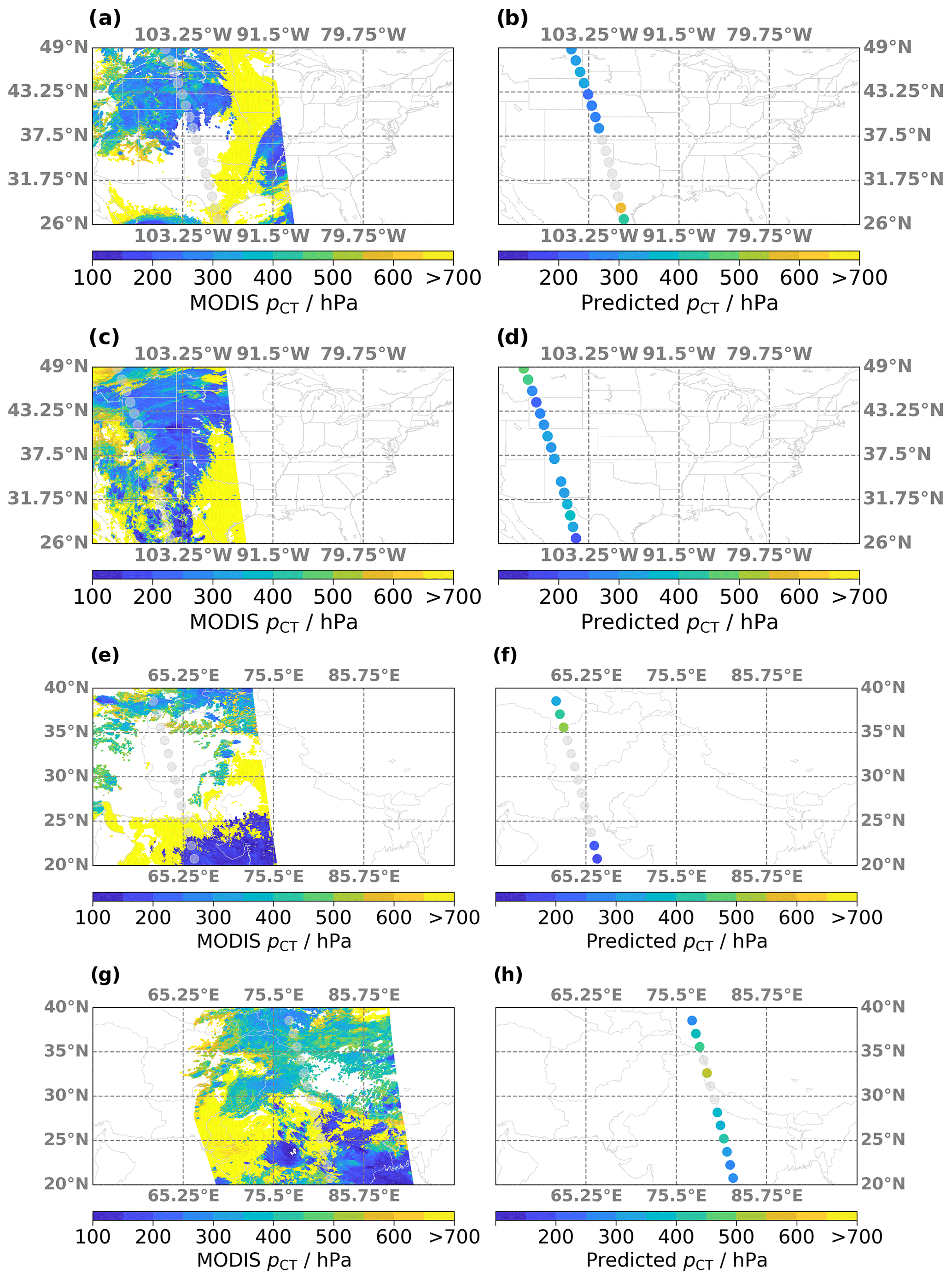
Figure 12(a) Map of cloud top pressure (pCT) retrieved from MODIS observations on 31 August 2017 over North America. Transparent circles indicate the MLS orbit. (b) Same as (a) but for the predicted pCT based on the ANN algorithm. (c, d) Same as (a, b) but for MLS and MODIS observations on 5 July 2015. (e, f) Similar to (a, b) but for MLS and MODIS observations on 28 June 2019. (g, h) Same as (a, b) but for MLS and MODIS observations on 5 July 2018.
5.3 Example scenes
Similar to the analysis in Sect. 4.4, comparisons between maps of MODIS-retrieved and predicted pCT for individual cloud fields provide a qualitative assessment of the model performance. MODIS results from the same four example scenes that were previously shown in Figs. 8 and 9 are presented in Fig. 12a, c, e, and f. The respective ANN predictions are shown in Fig. 12b, d, f, and h. The first two scenes are sampled over the North American monsoon region; the second two are over the Asian summer monsoon anticyclone.
The first example (panels a and b) consists of high clouds in the northern part of the scene, with the lowest pCT of ∼ 200 hPa around 40∘ latitude. The ANN reliably reproduces the MODIS results and predicts the highest clouds at the right position. Mixed results are achieved for the very low clouds in the south, which are outside of the MLS-detectable pressure range. For these two profiles, the ANN predicts pCT = 585 and 434 hPa. While clearly too low, the model successfully associates these samples with low clouds. The second scene (panels c and d) is characterized by high C values throughout, with low to mid-level clouds in the very north and a complicated mix of different cloud types throughout the rest of the scene. Not surprisingly, the ANN identifies all but three profiles to be associated with medium to high clouds. Here, even small occurrences of high clouds in the perimeter of an MLS profile yield a low pCT prediction.
Three samples in the vicinity of mid-level clouds are visible in the northern part of the third scene (panels e and f), as well as two profiles above very low and two profiles above high clouds in the south. While the ANN is not able to detect the pCT> 700 hPa region, it successfully predicts clouds with pCT = 343–511 hPa northward of 35∘ latitude and pCT< 206 hPa in the south. Finally, another complicated scene is depicted in panels g and h. The two southernmost profiles have a MODIS-observed pCT of 390 hPa and 285 hPa, which is accurately reproduced by the ANN. Predicted pCT for the three northernmost profiles agree similarly well with the observations. However, the ANN predictions are too low for profiles between 25 and 30∘ latitude and too high for the lone cloudy profile around 33∘ latitude.
As noted in Sect. 5.1–5.2, the performance for pCT predictions seems to decline with an increase in cloud top pressure, consistent with the reduced contrast between clear-sky and cloudy TB around pCT∼ 700 hPa, as shown in Fig. 3.
The current MLS cloud flags, reported in the Level 2 Geophysical Product files of version 4.2x, are designed to identify profiles that are influenced by significantly opaque clouds, with the main goal being to identify cases where retrieved composition profiles may have been adversely affected either by the clouds or by the steps taken in the retrieval to exclude cloud-affected radiances. In this study, we present an improved cloud detection scheme based on a standard multilayer perceptron, a subcategory of feedforward artificial neural networks (ANNs). It applies a softmax activation function in the output layer for binary classifications (i.e., clear sky or cloudy), while a log–loss function is minimized to determine the model weights. A second setup, which applies a linear output in the output layer and determines the model weights by minimizing the mean squared error, is used to produce a cloud top pressure (pCT) estimate from MLS radiances that approximates the MODIS retrievals. This new algorithm is shown not only to reliably detect high and mid-level convection containing even small amounts of cloud water but also to distinguish between high-reaching and mid-level to low convection.
To train the ANN models we colocated global MLS brightness temperatures (TB), sampled on 208 d between 2005 and 2020, with nadir-viewing MODIS-retrieved cloud properties aggregated within a 1∘ × 1∘ box (in latitude and longitude) around each MLS profile. This yielded a median cloud cover (C), pCT, and cloud water path (QT) associated with each of the 162 117 MLS scans in the colocated data set. These variables are used to discriminate clear-sky ( and QT< 25 g m−2) from cloudy (, 100 hPa ≤ pCT< 700 hPa, and QT> 50 g m−2) profiles. Overall, the input variables for the ANN consist of 1710 MLS-observed TB values from different spectral bands, channels, and minor frames (i.e., views at different altitudes in the atmosphere). After setting aside 10 % of the data to serve as an independent test data set, comprehensive testing and cross-validation procedures are conducted to identify the right set of hyperparameters (i.e., model settings). The ideal model parameters are used to train 100 different ANN models, where the colocated data are randomly shuffled and split into 70 % training and 20 % validation data (referenced to the size of the original data set). Three binary classification metrics are calculated for every model run to evaluate the cloud classification performance for unseen data: the accuracy (Ac), F1 score (F1), and Matthew's correlation coefficient (Mcc). Similarly, the Pearson product-moment correlation coefficient (r) and root mean square deviation (RMSD) provide the means to evaluate the performance of the pCT models. Average values and standard deviations from each set of 100 different model runs are , , , , and RMSD hPa. The high statistical scores and low variability in the results illustrate that the two ANN algorithms yield reliable cloud classifications and pCT estimates for previously unseen observations.
It is important to note that the predicted cloud parameters do not represent the true atmospheric state. Since each ANN was trained on the colocated MODIS targets, it follows that they, at best, will replicate the respective MODIS results. The MODIS retrievals, however, are characterized by their own uncertainties and biases, which are subsequently learned and reproduced by the derived models. This means that analyses of ANN performance in this study only provide an evaluation of how well each model can replicate the colocated MODIS retrievals.
A comparison with the current v4.2x status flags reveals that, for both the validation and test data sets, the new ANN results provide a significant improvement in cloud classification. The ANN algorithm correctly identifies > 93 % of cloudy profiles, while less than 6 % of the clear profiles are falsely flagged. In contrast, the current v4.2x flag detects only ∼16 % of cloudy profiles, and even though it is designed to identify sufficiently opaque clouds, it only correctly classifies < 27 % of cloudy profiles with QT> 1000 g m−2. The fraction of falsely flagged clear profiles is comparable to the ANN results. Apart from a reduced ability to detect clouds over regions with generally low cloud cover, no significant dependence on geolocation is observed, indicating that the ANN flag yields reliable classification results on a global scale. A global cloud cover map for data collected between 2005 and 2019 is presented, generated solely from MLS-sampled TB and the determined ANN weights. Typically observed cloud patterns and derived C agree reasonably well with MODIS results. Moreover, detailed examination of four example scenes from the North American and Asian summer monsoon regions reveals that the ANN can reliably identify diverse cloud fields, including those characterized by low clouds and low QT. Together with the consistently large statistical agreement, these global and regional examples of successful cloud detection illustrate that the predefined cloudiness conditions (following thresholds for C, pCT, and QT) are reasonable. Moreover, the uncertainties arising from associating MLS observations in the limb with nadir MODIS images do not seem to substantially impact the reliability of the ANN algorithm.
Similarly, the second ANN setup is able to reliably estimate the MODIS-retrieved pCT for profiles in the validation and test data set, with r>0.82 and RMSD < 80 hPa. It is shown that more than 66 % of pCT predictions are within 50 hPa of the MODIS results. Derived global maps of average ANN-predicted pCT can reproduce observed patterns in the MODIS retrievals. In particular, this model is able to correctly identify > 85 % of profiles with pCT< 400 hPa in the −60 to +60∘ latitude range. Conversely, the current v4.2x algorithm correctly flags only ∼ 9 % of such profiles as cloudy.
This new cloud classification scheme, which will be included in future versions of the MLS dataset, provides the means to reliably identify profiles with potential mid-level to high cloud influence. Note that MLS radiances are not affected by the change from v4.2x to v5.0x. As mentioned in the Introduction, this new algorithm will facilitate future research on reducing uncertainties in the retrieval of atmospheric constituents in the presence of clouds. Moreover, studies on convective moistening of the lowermost stratosphere, as well as cloud scavenging of atmospheric pollutants, will benefit from these new capabilities.
The following table lists the days included in the colocated MLS–MODIS data set. Days were semi-randomly chosen to ensure that each month is represented equally, and only complete measurement days (i.e., due to technical issues with the instruments) are included.
Table A1Details about the colocated MLS–MODIS data set, which contains observations from 13 random Julian days (d01–d13) for each year over 2005–2020.
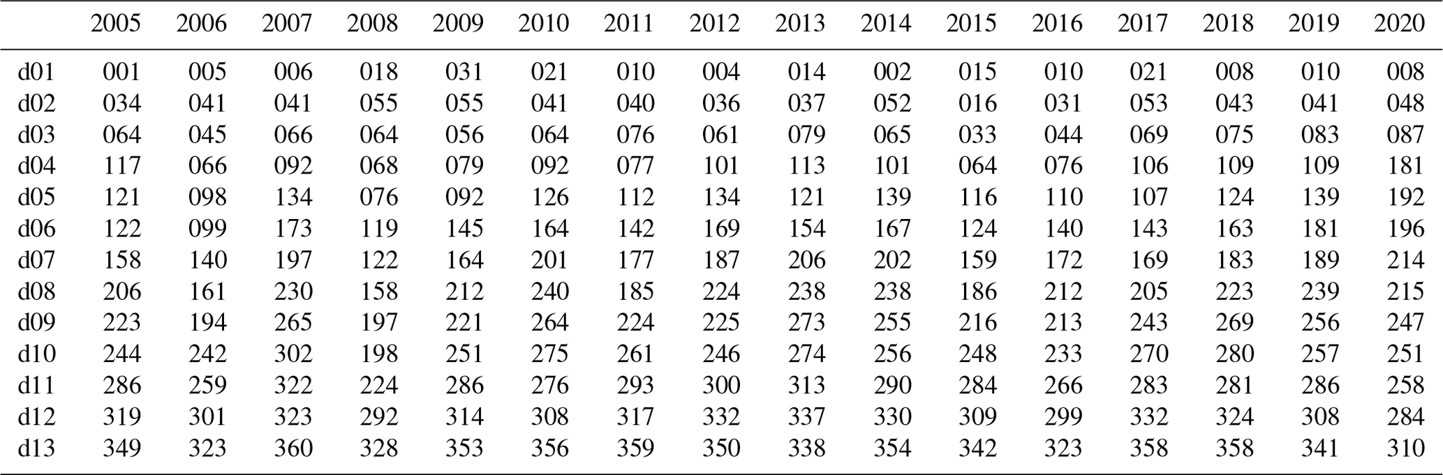
MLS brightness temperatures (https://doi.org/10.5067/Aura/MLS/DATA2009, Jarnot and Perun, 2020) and L2GP data, including status flags (e.g., https://doi.org/10.5067/Aura/MLS/DATA2009, Lambert et al., 2015 for the water vapor product), are publicly available at https://disc.gsfc.nasa.gov/ (last access: 24 November 2021).
Aqua MODIS cloud properties (https://doi.org/10.5067/MODIS/MYD06_L2.061, Platnick et al., 2015) are publicly available from NASA and the Atmosphere Archive and Distribution System (LAADS) (https://ladsweb.modaps.eosdis.nasa.gov/search/, last access: 24 November 2021).
All authors have shaped the concept of this study and refined the approach during extensive discussions. FW carried out the data analysis and wrote the initial draft of the manuscript, which was subsequently refined by all authors.
The contact author has declared that neither they nor their co-authors have any competing interests.
Publisher's note: Copernicus Publications remains neutral with regard to jurisdictional claims in published maps and institutional affiliations.
The authors acknowledge US Government sponsorship. The research was carried out at the Jet Propulsion Laboratory, California Institute of Technology, under a contract with the National Aeronautics and Space Administration.
This research has been supported by the National Aeronautics and Space Administration (grant no. 80NM0018D0004).
This paper was edited by Patrick Eriksson and reviewed by Carlos Jimenez and one anonymous referee.
Abadi, M., Agarwal, A., Barham, P., Brevdo, E., Chen, Z., Citro, C., Corrado, G. S., Davis, A., Dean, J., Devin, M., Ghemawat, S., Goodfellow, I., Harp, A., Irving, G., Isard, M., Jia, Y., Jozefowicz, R., Kaiser, L., Kudlur, M., Levenberg, J., Mane, D., Monga, R., Moore, S., Murray, D., Olah, C., Schuster, M., Shlens, J., Steiner, B., Sutskever, I., Talwar, K., Tucker, P., Vanhoucke, V., Vasudevan, V., Viegas, F., Vinyals, O., Warden, P., Wattenberg, M., Wicke, M., Yu, Y., and Zheng, X.: TensorFlow: Large-Scale Machine Learning on Heterogeneous Distributed Systems, arXiv [preprint], arXiv:1603.04467v2, 2016. a
Ackerman, S. A., Strabala, K. I., Menzel, W. P., Frey, R. A., Moeller, C. C., and Gumley, L. E.: Discriminating clear sky from clouds with MODIS, J. Geophys. Res., 103, 32141–32157, 1998. a
Ackerman, S. A., Holz, R. E., Frey, R., Eloranta, E. W., Maddux, B. C., and McGill, M.: Cloud Detection with MODIS. Part II: Validation, J. Atmos. Ocean. Techn., 25, 1073–1086, https://doi.org/10.1175/2007JTECHA1053.1, 2008. a
Anderson, J. G., Wilmouth, D. M., Smith, J. B., and Sayres, D. S.: UV Dosage Levels in Summer: Increased Risk of Ozone Loss from Convectively Injected Water Vapor, Science, 337, 835–839, https://doi.org/10.1126/science.1222978, 2012. a
Ardanuy, P. A., Han, D., and Salomonson, V. V.: The Moderate Resolution Imaging Spectrometer (MODIS), IEEE T. Geosci. Remote, 30, 2–27, 1992. a
Arking, A.: Latitudinal distribution of cloud cover from TIROS III photographs, Science, 143, 569–572, 1964. a
Arking, A. and Childs, J. D.: Retrieval of cloud cover parameters from multispectral satellite images, J. Clim. Appl. Meteorol., 24, 322–333, 1985. a
Barnes, W. L., Pagano, T. S., and Salomonson, V. V.: Prelaunch characteristics of the 'Moderate Resolution Imaging Spectroradiometer' (MODIS) on EOS–AM1, IEEE T. Geosci. Remote, 36, 1088–1100, 1998. a
Brenguier, J.-L., Pawlowska, H., Schüller, L., Preusker, R., Fischer, J., and Fouquart, Y.: Radiative properties of boundary layer clouds: Droplet effective radius versus number concentration, J. Atmos. Sci., 57, 803–821, 2000. a
Chollet, F. and Keras Team: Keras, available at: https://keras.io (last access: 24 November), 2015. a
Clapp, P. F.: Global cloud cover for seasons using TIROS nephanalyses, Mon. Weather Rev., 92, 495–507, 1964. a
COESA: U.S. Standard Atmosphere, NASA-TM-X-74335, U.S. Government Printing Office, Washington, DC, October 1976. a
Goodfellow, I., Bengio, Y., and Courville, A.: Deep Learning (Adaptive Computation and Machine Learning series), MIT Press, Cambridge, MA, 2016. a
Han, Q., Rossow, W., and Lacis, A.: Near-global survey of effective droplet radii in liquid water clouds using ISCCP data, J. Climate, 7, 465–497, 1994. a
Jarnot, R. and Perun, V.: MLS/Aura L1 Radiances from Filter Banks for GHz V005, Goddard Earth Sciences Data and Information Services Center (GES DISC) [data set], Greenbelt, MD, USA, https://doi.org/10.5067/Aura/MLS/DATA1503, 2020 (data available at: https://disc.gsfc.nasa.gov/, last access: 24 November 2021). a
Jeppesen, J. H., Jacobsen, R. H., Inceoglu, F., and Toftegaard, T. S.: A cloud detection algorithm for satellite imagery based on deep learning, Remote Sens. Environ., 229, 247–259, https://doi.org/10.1016/j.rse.2019.03.039, 2019. a
Kaufman, Y. J. and Nakajima, T.: Effect of Amazon smoke on cloud microphysics and albedo – Analysis from satellite imagery, J. Appl. Meteorol., 32, 729–744, 1993. a
King, M. D., Platnick, S., Wenzel, W. P., Ackerman, S. A., and Hubanks, P. A.: Spatial and Temporal Distribution of Clouds Observed by MODIS Onboard the Terra and Aqua Satellites, IEEE T. Geosci. Remote, 51, 3826–3852, https://doi.org/10.1109/TGRS.2012.2227333, 2013. a
Krämer, M., Schiller, C., Ziereis, H., Ovarlez, J., and Bunz, H.: Nitric acid partitioning in cirrus clouds: the role of aerosol particles and relative humidity, Tellus B, 58B, 141–147, https://doi.org/10.3402/tellusb.v58i2.16805, 2006. a
Lacagnina, C. and Selten, F.: Evaluation of clouds and radiative fluxes in the EC-Earth general circulation model, Clim. Dynam., 43, 2777–2796, https://doi.org/10.1007/s00382-014-2093-9, 2014. a
Lambert, A., Read, W., and Livesey, N.: MLS/Aura Level 2 Water Vapor (H2O) Mixing Ratio V004, Goddard Earth Sciences Data and Information Services Center (GES DISC) [data set], Greenbelt, MD, USA, https://doi.org/10.5067/Aura/MLS/DATA2009, 2015 (data available at: https://disc.gsfc.nasa.gov/, last access: 24 November 2021). a
LeCun, Y., Boser, B., Denker, J. S., Henderson, D., Howard, R. E., Hubbard, W., and Jackel, L. D.: Backpropagation Applied to Handwritten Zip Code Recognition, Neural Comput., 1, 541–551, 1989. a
LeCun, Y. A., Bottou L., Orr, G. B., and Müller, K. R.: Efficient BackProp, in: Neural Networks: Tricks of the Trade. Lecture Notes in Computer Science, vol. 7700, edited by: Montavon, G., Orr, G. B., and Müller, K. R., Springer, Berlin, Heidelberg, https://doi.org/10.1007/978-3-642-35289-8_3, 2012. a
Livesey, N. J., Read, W. G., Wagner, P. A., Froidevaux, L., Lambert, A., Manney, G. L., Valle, L. F. M., Pumphrey, H. C., Santee, M. L., Schwartz, M. J., Wang, S., Fuller, R. A., Jarnot, R. F., Knosp, B. W., Martinez, E., and Lay, R. R.: Version 4.2x Level 2 and 3 data quality and description document., Tech. Rep. JPL D-33509 Rev. E, Jet Propulsion Laboratory, California Institute of Technology, Pasadena, California, 91109-8099, 2020. a, b, c
Menzel, W. P., Frey, R. A., Zhang, H., Wylie, D. P., Moeller, C. C., Holz, R. E., Maddux, B., Baum, B. A., Strabala, K. I., and Gumley, L. E.: MODIS global cloud-top pressure and amount estimation: Algorithm description and results, J. Appl. Meteorol. Clim., 47, 1175–1198, 2008. a
Miller, D. J., Zhang, Z., Ackerman, A. S., Platnick, S., and Baum, B. A.: The impact of cloud vertical profile on liquid water path retrieval based on the bispectral method: A theoretical study based on large-eddy simulations of shallow marine boundary layer clouds, J. Geophys. Res., 121, 4122–4141, https://doi.org/10.1002/2015JD024322, 2016. a
Minnis, P., Heck, P., Young, D., Fairall, C., and Snider, J.: Stratocumulus cloud properties derived from simultaneous satellite and island-based instrumentation during FIRE, J. Appl. Meteorol., 31, 317–339, 1992. a
Muhlbauer, A., McCoy, I. L., and Wood, R.: Climatology of stratocumulus cloud morphologies: microphysical properties and radiative effects, Atmos. Chem. Phys., 14, 6695–6716, https://doi.org/10.5194/acp-14-6695-2014, 2014. a
Platnick, S. and Twomey, S.: Determining the susceptibility of cloud albedo to changes in droplet concentration with the Advanced Very High Resolution Radiometer, J. Appl. Meteorol., 33, 334–347, 1994. a
Platnick, S., King, M., Wind, G., Ackerman, S., Menzel, P., and Frey, R.: MODIS/Aqua Clouds 5-Min L2 Swath 1km and 5km, NASA MODIS Adaptive Processing System [data set], Goddard Space Flight Center, USA, https://doi.org/10.5067/MODIS/MYD06_L2.061, 2015 (data available at: https://ladsweb.modaps.eosdis.nasa.gov/search/, last access: 24 November 2021). a
Platnick, S., Meyer, K. G., King, M. D., Wind, G., Amarasinghe, N., Marchant, B., Arnold, G. T., Zhang, Z., Hubanks, P. A., Holz, R. E., Yang, P., Ridgway, W. L., and Riedi, J.: The MODIS cloud optical and microphysical products: Collection 6 updates and examples from Terra and Aqua, IEEE T. Geosci. Remote, 55, 502–525, https://doi.org/10.1109/TGRS.2016.2610522, 2017. a
Ramanathan, V., Cess, R. D., Harrison, E. F., Minnis, P., Barkstrom, B. R., Ahmad, E., and Hartmann, D. L.: Cloud–Radiative Forcing and Climate: Results from the Earth Radiation Budget Experiment, Science, 243, 57–63, 1989. a
Ratté-Fortin, C., Chokmani, K., and El-Alem, A.: A novel algorithm of cloud detection for water quality studies using 250 m downscaled MODIS imagery, Int. J. Remote Sens., 39, 6429–6439, https://doi.org/10.1080/01431161.2018.1460506, 2018. a
Reed, R. and Marks, R. J.: Neural Smithing: Supervised Learning in Feedforward Artificial Neural Networks, The MIT Press, https://doi.org/10.7551/mitpress/4937.001.0001, 1999. a
Rossow, W. B., Kinsella, E., and Garder, L.: Seasonal and global cloud variations deduced from polar orbiting satellite radiance measurements, in: Proc. Fifth Conf. on Atmospheric Radiation, Baltimore, 31 October–4 November 1983, Baltimore, MD, Am. Meteorol. Soc., 195–198, 1983. a
Saponaro, G., Kolmonen, P., Karhunen, J., Tamminen, J., and de Leeuw, G.: A neural network algorithm for cloud fraction estimation using NASA-Aura OMI VIS radiance measurements, Atmos. Meas. Tech., 6, 2301–2309, https://doi.org/10.5194/amt-6-2301-2013, 2013. a, b
Schwartz, M. J., Read, W. G., Santee, M. L., Livesey, N. J., Froidevaux, L., Lambert, A., and Manney, G. L.: Convectively injected water vapor in the North American summer lowermost stratosphere, Geophys. Res. Lett., 40, 2316–2321, https://doi.org/10.1002/grl.50421, 2013. a
Stephens, G.: Cloud feedbacks in the climate system: A critical review, J. Climate, 18, 237–273, 2005. a
Sun, L., Yang, X., Jia, S., Jia, C., Wang, Q., Liu, X., Wei, J., and Zhou, X.: Satellite data cloud detection using deep learning supported by hyperspectral data, Int. J. Remote Sens., 41, 1349–1371, https://doi.org/10.1080/01431161.2019.1667548, 2020. a
Tinney, E. N. and Homeyer, C. R.: A 13-year Trajectory-Based Analysis of Convection-Driven Changes in Upper Troposphere Lower Stratosphere Composition over the United States, J. Geophys. Res.-Atmos., 126, e2020JD033657, https://doi.org/10.1029/2020JD033657, 2020. a, b
Varnai, T. and Marshak, A.: Satellite Observations of Cloud-Related Variations in Aerosol Properties, Atmosphere, 9, 430, https://doi.org/10.3390/atmos9110430, 2018. a
Wang, T., Shi, J., Letu, H., Ma, Y., Li, X., and Zheng, Y.: Detection and Removal of Clouds and Associated Shadows in Satellite Imagery Based on Simulated Radiance Fields, J. Geophys. Res.-Atmos., 124, 7207–7225, https://doi.org/10.1029/2018JD029960, 2019. a
Warren, S. G., Hahn, C. H., London, J., Chervin, R. M., and Jenne, R. L.: Global Distribution of Total Cloud Cover and Cloud Type Amounts Over the Ocean, University Corporation for Atmospheric Research, Technical Report No. NCAR/TN-317+STR, https://doi.org/10.5065/D6QC01D1, 1988. a
Waters, J. W., Froidevaux, L., Harwood, R. S., Jarnot, R. F., Pickett, H. M., Read, W. G., Siegel, P. H., Cofield, R. E., Filipiak, M. J., Flower, D. A., Holden, J. R., Lau, G. K., Livesey, N. J., Manney, G. L., Pumphrey, H. C., Santee, M. L., Wu, D. L., Cuddy, D. T., Lay, R. R., Loo, M. S., Perun, V. S., Schwartz, M. J., Stek, P. C., Thurstans, R. P., Boyles, M. A., Chandra, K. M., Chavez, M. C., Gun-Shing Chen, Chudasama, B. V., Dodge, R., Fuller, R. A., Girard, M. A., Jiang, J. H., Yibo Jiang, Knosp, B. W., LaBelle, R. C., Lam, J. C., Lee, K. A., Miller, D., Oswald, J. E., Patel, N. C., Pukala, D. M., Quintero, O., Scaff, D. M., Van Snyder, W., Tope, M. C., Wagner, P. A., and Walch, M. J.: The Earth observing system microwave limb sounder (EOS MLS) on the aura Satellite, IEEE T. Geosci. Remote, 44, 1075–1092, https://doi.org/10.1109/TGRS.2006.873771, 2006. a, b
Werner, F., Wind, G., Zhang, Z., Platnick, S., Di Girolamo, L., Zhao, G., Amarasinghe, N., and Meyer, K.: Marine boundary layer cloud property retrievals from high-resolution ASTER observations: case studies and comparison with Terra MODIS, Atmos. Meas. Tech., 9, 5869–5894, https://doi.org/10.5194/amt-9-5869-2016, 2016. a
Werner, F., Schwartz, M. J., Livesey, N. J., Read, W. G., and Santee, M. L.: Extreme Outliers in Lower Stratospheric Water Vapor Over North America Observed by MLS: Relation to Overshooting Convection Diagnosed From Colocated Aqua-MODIS Data, Geophys. Res. Lett., 47, e2020GL090131, https://doi.org/10.1029/2020GL090131, 2020. a, b, c
Wu, D. L., Jiang, J. H., and Davis, C. P.: EOS MLS cloud ice measurements and cloudy-sky radiative transfer model, IEEE T. Geosci. Remote, 44, 1156–1165, https://doi.org/10.1109/TGRS.2006.869994, 2006. a, b, c
Wu, D. L., Jiang, J. H., Read, W. G., Austin, R. T., Davis, C. P., Lambert, A., Stephens, G. L., Vane, D. G., and Waters, J. W.: Validation of the Aura MLS cloud ice water content measurements, J. Geophys. Res., 113, D15S10, https://doi.org/10.1029/2007JD008931, 2008. a
Wurzler, S., Flossmann, A. I., Pruppacher, H. R., and Schwartz, S. E.: The scavenging of nitrate by clouds and precipitation, J. Atmos. Chem., 20, 259–280, https://doi.org/10.1007/BF00694497, 1995. a
Yang, Y. and Di Girolamo, L.: Impacts of 3-D radiative effects on satellite cloud detection and their consequences on cloud fraction and aerosol optical depth retrievals, J. Geophys. Res., 113, D04213, https://doi.org/10.1029/2007JD009095, 2008. a
Yu, W., Dessler, A. E., Park, M., and Jensen, E. J.: Influence of convection on stratospheric water vapor in the North American monsoon region, Atmos. Chem. Phys., 20, 12153–12161, https://doi.org/10.5194/acp-20-12153-2020, 2020. a
Zhao, G. and Di Girolamo, L.: Statistics on the macrophysical properties of trade wind cumuli over the tropical western Atlantic, J. Geophys. Res., 112, D10204, https://doi.org/10.1029/2006JD007371, 2007. a
- Abstract
- Copyright statement
- Introduction
- Data
- Artificial neural network
- Cloud detection: results and examples
- Predicting cloud top pressure: results and examples
- Summary and conclusions
- Appendix A: Days in the MLS–MODIS data set
- Data availability
- Author contributions
- Competing interests
- Disclaimer
- Acknowledgements
- Financial support
- Review statement
- References