the Creative Commons Attribution 4.0 License.
the Creative Commons Attribution 4.0 License.
 | 02 Feb 2021
Real-time measurement of radionuclide concentrations and its impact on inverse modeling of 106Ru release in the fall of 2017
Miroslav Hýža
Nikolaos Evangeliou
Václav Šmídl
Low concentrations of 106Ru were detected across Europe at the turn of September and October 2017. The origin of 106Ru has still not been confirmed; however, current studies agree that the release occurred probably near Mayak in the southern Urals. The source reconstructions are mostly based on an analysis of concentration measurements coupled with an atmospheric transport model. Since reasonable temporal resolution of concentration measurements is crucial for proper source term reconstruction, the standard 1-week sampling interval could be limiting. In this paper, we present an investigation of the usability of the newly developed AMARA (Autonomous Monitor of Atmospheric Radioactive Aerosol) and CEGAM (carousel gamma spectrometry) real-time monitoring systems, which are based on the gamma-ray counting of aerosol filters and allow for determining the moment when 106Ru arrived at the monitoring site within approx. 1 h and detecting activity concentrations as low as several mBq m−3 in 4 h intervals. These high-resolution data were used for inverse modeling of the 106Ru release. We perform backward runs of the Hybrid Single-Particle Lagrangian Integrated Trajectory (HYSPLIT) atmospheric transport model driven with meteorological data from the Global Forecast System (GFS), and we construct a source–receptor sensitivity (SRS) matrix for each grid cell of our domain. Then, we use our least squares with adaptive prior covariance (LS-APC) method to estimate possible locations of the release and the source term of the release. With Czech monitoring data, the use of concentration measurements from the standard regime and from the real-time regime is compared, and a better source reconstruction for the real-time data is demonstrated in the sense of the location of the source and also the temporal resolution of the source. The estimated release location, Mayak, and the total estimated source term, 237±107 TBq, are in agreement with previous studies. Finally, the results based on the Czech monitoring data are validated with the IAEA-reported (International Atomic Energy Agency) dataset with a much better spatial resolution, and the agreement between the IAEA dataset and our reconstruction is demonstrated. In addition, we validated our findings also using the FLEXPART (FLEXible PARTicle dispersion) model coupled with meteorological analyses from the European Centre for Medium-Range Weather Forecasts (ECMWF).
- Article
(5192 KB) - Full-text XML
-
Supplement
(129 KB) - BibTeX
- EndNote


At the turn of September and October 2017, low concentrations of 106Ru of unknown origin were detected in the atmosphere in the Czech Republic. Immediate communication with other European laboratories involved in the RO5 (Ring of Five) network (Masson et al., 2011) confirmed that this was a Europe-wide occurrence. Although the concentration was low (tens of mBq m−3) and was of no health risk, the unknown origin of 106Ru raised concerns. Therefore, very shortly after the first detections, efforts were made to estimate the source location based on the RO5 data. Initial analyses pointed to a possible source located to the east of the Czech Republic. As the dataset grew, this estimate was refined to the Ural region as the most probable location (Kovalets and Romanenko, 2017). The released 106Ru activity was estimated to be several hundred TBq (Saunier et al., 2019; Western et al., 2020).
Since 106Ru is a fission product produced in a nuclear reactor, the question arose about the nature of the source. A nuclear reactor accident was rejected because, in this case, other radionuclides would have been detected besides 106Ru, as during the Chernobyl nuclear power plant (NPP) accident (UNSCEAR, 2000). For example, during post-Chernobyl monitoring, the detected 106Ru was higher by 2 or 3 orders of magnitude and was accompanied by a complex mix of radionuclides, including 131I, 132Te, 137Cs, 134Cs, 140La, and 103Ru (Chz, 1987).
Other working hypotheses included the melting of a radioisotope thermoelectric generator (RTG) or of a medical source, since 106Ru is used in medicine for the treatment of ophthalmic tumors (Takiar et al., 2015). In several samples where the 106Ru activity was relatively high, we also detected 103Ru isotope but at much lower concentrations. The activity ratio of was approx. 4000 (after the Chernobyl accident, the ratio was approximately 0.12), which suggests that the ruthenium was extracted from relatively fresh nuclear fuel (approximately 2 years old). Since medical sources and RTG would explain neither the occurrence of 106Ru nor the large source of several hundred TBq, fresh nuclear fuel is the most likely candidate.
In the end, an industrial source was identified as the most probable explanation – most likely a fuel reprocessing plant. This conclusion is supported by historical evidence, since we have observed several such events in the past – Tomsk (Tcherkezian et al., 1995), Savannah River (Carlton and Denham, 1997), and La Hague (ACRO, 2002). Based on these reports, it can be concluded that a selective release of 106Ru is possible during certain stages of fuel reprocessing or vitrification of fuel in the form of highly volatile RuO4 which can escape into the environment even when aerosol filters are employed. RuO4 then condenses in the colder air and can be further transported over long distances attached to atmospheric aerosol. There are two known plants in the southern Ural region which come into consideration – Mayak and Dimitrovgrad. Both are located within the region estimated by atmospheric transport modeling (ATM). Moreover, measurements performed by Roshydromet (Russian Federal Service for Hydrometeorology and Environmental Monitoring) confirm a positive detection of 106Ru in aerosols and in the fallout in the Chelyabinsk region (Shershakov et al., 2019).
Multiple investigations using different datasets and methodologies have now been performed with the same conclusion, indicating the Mayak plant as the probable source location (Masson et al., 2019; Saunier et al., 2019; Maffezzoli et al., 2019; De Meutter et al., 2020; Le Brazidec et al., 2020). Masson et al. (2019) presented a comprehensive event analysis, including a detailed radioruthenium forensic investigation, and speculated on the possibility of 106Ru release during the production of the 144Ce source for the SOX (short distance neutrino oscillations with Borexino) project at the Gran Sasso National Laboratory (also suggested by Bossew et al., 2019). Nonetheless, the Russian authorities deny any leakage from the Mayak plant (Nikitina and Slobodenyuk, 2018). Current estimates of 106Ru source location and source term are mainly based on an analysis of ambient measurements of 106Ru concentrations.
There is always a trade-off between sensitivity and timely reporting of concentration results, and the standard procedure provides a rather poor time resolution of the concentration monitoring data for the purposes of ATM analyses. The time delay between the possible arrival of the contamination at the monitoring site and its detection can easily be as long as 1 week. Long-term shortening of the sampling interval below 1 d is virtually unachievable, mainly for logistic reasons.
This limitation is of great research interest at the National Radiation Protection Institute (NRPI), Czech Republic, where near real-time monitoring systems (AMARA and CEGAM; see Sect. 2 for a detailed description ) are currently under development. Both systems yield minimum detectable activity (MDAC) at a level of 1 mBq m−3, which was sufficient to detect 106Ru during the 2017 episode. We were able to perform an experimental run of the AMARA device, and we managed to detect the exact moment when the contamination arrived. These real-time monitoring data were then used for source localization, and the results were compared with the standard time resolution. For this purpose, we use a Bayesian inversion method, called the least squares with an adaptive prior covariance (LS-APC) method (Tichý et al., 2016), which was later extended also for the source location problem (Tichý et al., 2017).
Our aim is to use the data from the Czech Radiation Monitoring Network to investigate two points. First, we will study the influence of the real-time monitoring data on the resulting estimate of the temporal profile of the emission. Our hypothesis is that the use of real-time monitoring data should lead to more time-specific estimates. Second, we will investigate and discuss what information can be estimated from the Czech monitoring data only. This task is very challenging, since it implies a very sparse monitoring network due to the small area of the Czech Republic in comparison with the relevant Eurasian spatial domain. The results will be validated and will be compared with results of the much larger International Atomic Energy Agency (IAEA) dataset (IAEA, 2017).
2.1 Standard sampling and measurement procedure
In the Czech Radiation Monitoring Network (RMN), aerosol samples are taken from 10 permanent monitoring sites which are equipped with high-volume aerosol samplers with a flow rate in the range of 150–900 m3 h−1. In addition to these monitoring sites, radionuclides are also monitored in the local networks in the vicinity of the nuclear power plants in the Czech Republic – these data are not included in the analysis.
The standard sampling frequency is usually once or twice a week. Combined weekly samples are subjected to semiconductor gamma spectrometry, with no further treatment, at four RMN laboratories. Preliminary measurement of aerosol filters starts a few hours after the end of the sampling to allow time for the short-lived radon progenies to decay. Otherwise, they would significantly affect the measurement sensitivity. The preliminary measurements last approximately 5 h, after which the detection limit (minimum detectable activity – MDAC) is at a level of 10 µBq m−3. Consequently, a detailed measurement lasting approx. 5 d is performed, after which the sub-µBq m−3 MDAC level is achieved.
106Ru is a β emitter and therefore cannot itself be detected by means of gamma-ray spectrometry. 106Ru activity is determined on the basis of its short-lived progeny 106Rh, which emits several gamma rays of convenient energy and intensity (622 and 1050 keV being the most prominent). In order to determine the activity accurately, it is necessary to correct for true coincidence effects, as 106Rh emits gamma photons in cascades. By failing to do this, one can easily underestimate the activity by 15 %–20 %.
2.2 Real-time sampling and measurement procedure
2.2.1 AMARA system
The AMARA system employs a fully continuous measurement regime where the aerosol filter is counted via gamma-ray spectrometry already during sampling using a high-volume (900 m3 h−1) sampler. In this setup, shown in Fig. 1, a spectrometric module consisting of a high-purity germanium (HPGe) detector is placed directly above the aerosol filter. This straightforward solution benefits from its simplicity and from the real-time nature of the measurement. However, the detection limits are higher due to the very high and variable natural background caused mainly by 222Rn and 220Rn decay products. Our approach for suppressing the high and widely variable radon background is based on the NASVD (Noise Adjusted Singular Value Decomposition) algorithm (Minty and Hovgaard, 2002) and consists of extracting the characteristic spectral shapes from a large dataset of background measurements. We adopted this approach already in the previous version of the AMARA system, which was based on a NaI (Tl) detector. The implementation details are described by Hýža and Rulík (2017), and a demonstration of the signal treatment is displayed in Fig. 2.

Figure 1AMARA system schematics; the activity deposition is measured using an HPGe detector above an aerosol filter during sampling. LAN: local area network.
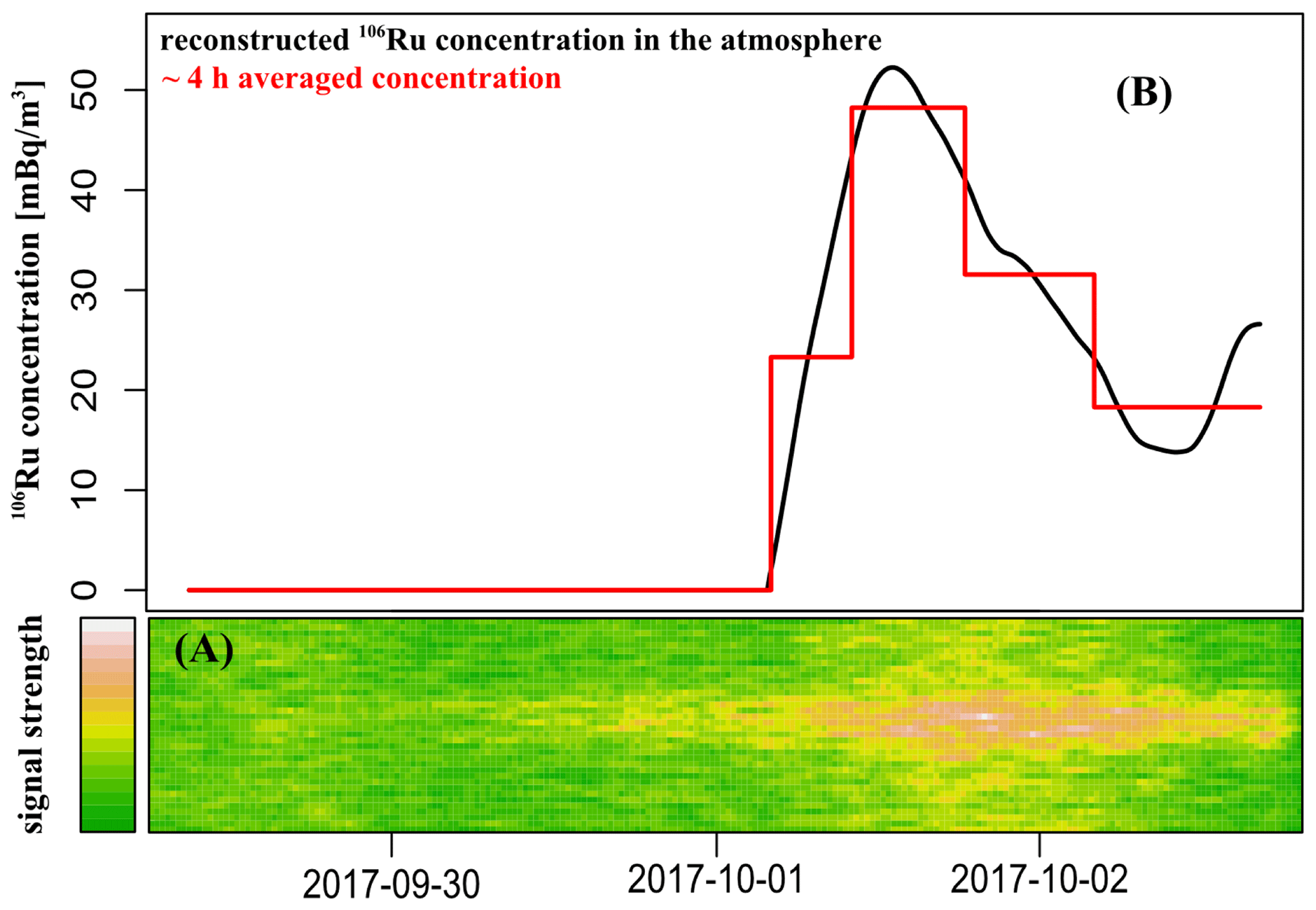
Figure 2The response of the AMARA system to the 106Ru contamination passing over during the corresponding sampling interval. (a) The 106Ru signal increase in the 615–630 keV energy region after subtracting the radon background. (b) The example reconstructed real-time 106Ru concentration and its 4 h averaged values, which corresponds to the CEGAM time resolution. Please note that the date format in this figure is year month day (yyyy-mm-dd).
2.2.2 CEGAM system
The CEGAM system is based on semicontinuous sampling where samples are taken at preset intervals and then measured via gamma spectrometry. The device is based on a carousel sampling changer, which moves the aerosol filters between the sampling position and the measuring position; see the configuration in Fig. 3. This allows for the CEGAM’s HPGe spectrometer to be placed inside a heavy lead shielding, and it is also possible to let the radon progenies decay before the measurement. The natural background level is therefore much lower in comparison with the AMARA system, and it yields similar MDAC values but at a much lower flow rate (10 m3 h−1).
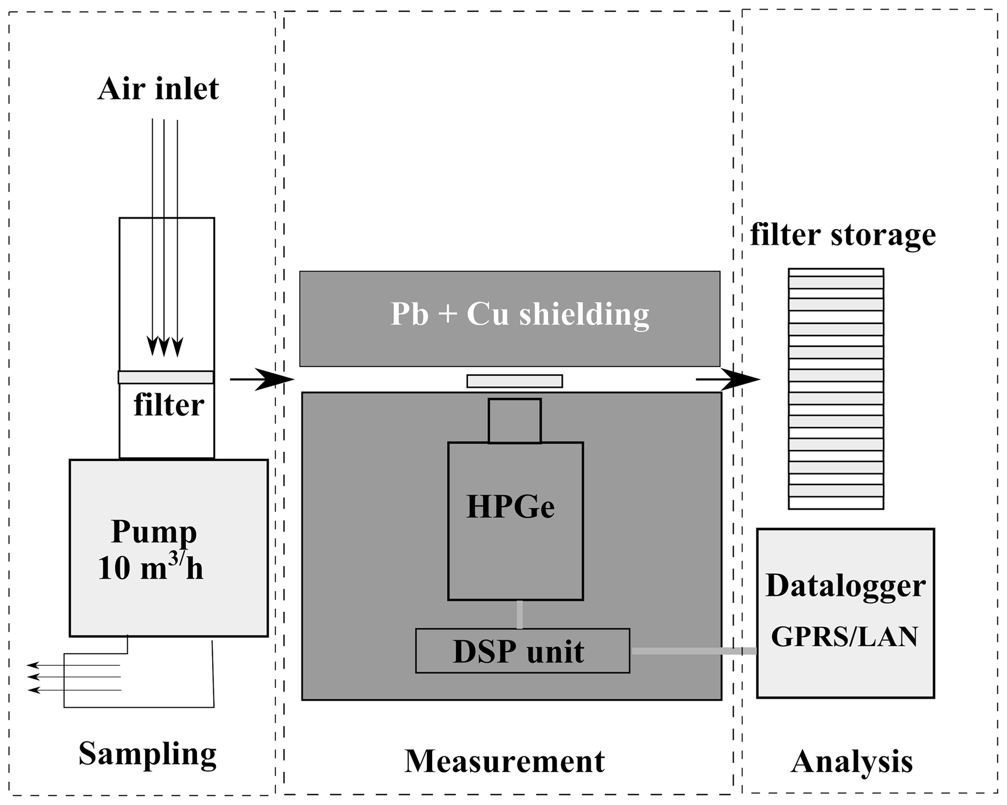
Figure 3CEGAM system schematics. The activity deposition is measured using an HPGe detector above an aerosol filter after sampling in radiation shielding. LAN: local area network; DSP: digital signal processing; GPRS: general packet radio service.
2.2.3 Measurement procedure and system comparison
Both the AMARA and CEGAM systems employ an electrically cooled HPGe (Ortec–Canberra) detector in a temperature- and humidity-controlled environment in order to ensure smooth continuous operation even during demanding weather conditions. The signal processing is done by digital multi-channel (DSPEC–Lynx) analyzer. The eventual gain shift is automatically corrected by a stabilization algorithm based on the position of background peaks. The efficiency calibrations were done experimentally using aerosol filters spiked with standard activity solutions provided by the Czech Metrology Institute. For the purpose of calibration and measurement respectively, the correction to the true coincidence summation was taken into account. As the AMARA system operates in a continuous regime, the spectrum acquisition time was set to 5 min in order to make full use of its time resolution. Consequently, the running spectral sums of arbitrary lengths can be constructed. The actual activity values are then computed using the numerical derivative of smoothed cumulative response. On the other hand, the time resolution of the CEGAM system is limited by the carousel changer time steps. Typically, the spectrum acquisition time is set to 24 h, and in case of emergency it is shortened to 4 h or less.
The inherent time resolution of the monitoring system is inevitably related to the accuracy of the contamination arrival time. For the 106Ru case, the AMARA system estimated its arrival with approx. 1 h accuracy depending on the chosen level of statistical significance and the type of statistical test.
Although the detector efficiency and flow rate are determined relatively accurately, there are other effects negatively influencing the final activity uncertainty. For instance, the radon decay product concentration and therefore the MDAC and the activity uncertainty vary significantly. In case of positive detection, there is also an additional uncertainty contribution due to the deposition dynamics, as the system needs to subtract the contribution from the already deposited contamination. Comparing the real-time values with those obtained by laboratory measurements (106Ru case or natural 7Be), we estimate the uncertainty of (10–15) % for the 4 h integration time and the activity of several mBq m−3.
Although both systems are intended for the rapid detection of artificial radionuclides in the air, they differ in their typical use. The CEGAM system is an autonomous system with a high filter capacity, and it is suitable for remote places with difficult access for the operating personnel. The power consumption is also much lower in comparison with the AMARA system due to the employment of a low-volume sampler with an adjustable throughput. During a normal situation, the CEGAM system could be used within a monitoring network as a standby device (low flow rate and long sampling intervals) which could quickly switch to an emergency mode (higher flow rate and more frequent sampling). The switching command could be based on some prior information about arriving contamination or on the positive detection in a laboratory or by a more sensitive or rapid device, such as the AMARA system.
The AMARA system is intended to be an upgrade to an already existing monitoring site equipped with a high-volume sampler with operational personnel because the filters are not changed automatically. The advantage of this approach is a better time resolution and therefore rapid response. Monitoring sites with high-volume samplers are usually equipped with a gamma-ray spectrometry laboratory, and therefore the filters from AMARA are consequently measured in a dedicated counting room and potentially investigated further by radiochemical procedures to determine the activities of non-gamma-ray emitters. The proximity of the laboratory also solves to a certain degree the dilemma between the sensitivity of measurement and sampling duration, as the final most sensitive measurement will be performed in a laboratory after the sampling using the standard analytic procedure.
Table 1Technical specification of the AMARA and CEGAM systems. FWHM: full width at half maximum.
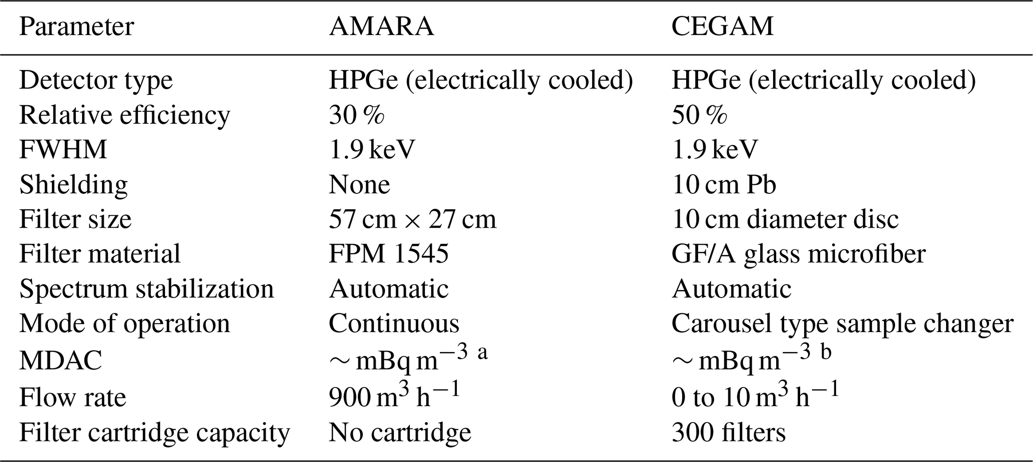
a Integration time of 1 h and 12 h of sampling. b Per 4 h sampling–measurement period.
Both systems together provide a very good solution for rapid radiation monitoring response to various release scenarios. The technical parameters are summarized in Table 1.
2.3 Dataset description
The monitoring data come from 10 standard monitoring sites in the Czech Republic from the time period between 25 September 2017 and 13 October 2017. Once 106Ru was confirmed by the AMARA system (located in Prague), the filters were changed, and the monitoring interval was shortened at all monitoring sites. The previous, less sensitive version of the AMARA system equipped with a NaI (Tl) spectrometer operated in the Hradec Králové location. Unfortunately, the CEGAM system was not yet operational during the 106Ru incident; hence, all used data come from the AMARA system.
A total of 47 samples were collected, and 24 of them were positive results with reported activity above the MDAC level. Four distinct datasets were derived on the basis of this monitoring campaign:
-
The RAW dataset comprises raw monitoring, as reported by the individual standard monitoring sites. The real-time measurements are not included.
-
The WEEKS dataset is derived from the raw dataset by weekly averaging. This dataset corresponds to the standard RMN monitoring regime.
-
The FAST dataset comprises raw data complemented by real-time values from the AMARA and CEGAM (simulated) systems. The integration window was set within the interval of 3–13 h during the concentration peak period.
-
The CUT dataset is created by cutting off the time interval between the start of sampling and the arrival of the 106Ru contamination at the particular monitoring site. As there was no real-time measurement apart from the Prague and Hradec Králové AMARA measurements, the arrival times were estimated on the basis of an overall analysis of the atmospheric transport across the Czech Republic, using the Hybrid Single-Particle Lagrangian Integrated Trajectory (HYSPLIT) model.
Note that the artificial WEEKS and CUT datasets are derived from the RAW and FAST datasets and are rather experimental. All four datasets are attached as a Supplement to this article.
For illustration, the measurements from the Prague station (equipped by the AMARA system) are given in Fig. 4, where much better temporal specificity is demonstrated.

Figure 4The measurements from the Prague station are displayed for each dataset using coloring given in the legend.
The general purpose of inverse atmospheric modeling is to estimate the time profile of an unknown emission, called the source term, in the so-called top-down approach (Nisbet and Weiss, 2010), where ambient measurements are combined with the result of an atmospheric transport model (ATM). The source term can be estimated using optimization of the differences between the measurements and the corresponding simulated values predicted by an ATM. An even more challenging task is to identify the location of the release. This can be done, e.g., using possible source location selection and comparison as in the case of the 131I release in January–February 2017 (Masson et al., 2018), using computed correlation or cost function maps as in the case of radioxenon after the third North Korean nuclear test (De Meutter et al., 2018), or using a Bayesian approach as in the case of the 131I release in the fall of 2011 (Tichý et al., 2017) or in the case of the 75Se leakage in 2019 (De Meutter and Hoffman, 2020).
In this paper, we follow the general concept of a linear model of the atmospheric dispersion using a source–receptor sensitivity (SRS) matrix (e.g., Seibert, 2001; Seibert and Frank, 2004). Here, an atmospheric transport model is used to calculate the linear relation between the potential source and the measured concentrations. Aggregating all possible time steps of the release in a source term vector x∈Rn and measurements from all sites and times in the vector y∈Rp, we can define the model
where is the SRS matrix and e∈Rp is an observation error, where the model errors and the measurements errors are aggregated. This concept has been largely used previously to recover the source term within larger-scale scenarios such as nuclear power plant accidents (Stohl et al., 2012; Evangeliou et al., 2017), estimates of the emission of greenhouse gases (Stohl et al., 2009), or volcanic emission (Kristiansen et al., 2010).
The estimation of the source term vector x from Eq. (1) is non-trivial, since the SRS matrix M is typically ill-conditioned and some regularization is needed. One possible approach is to minimize a suitable cost function (Eckhardt et al., 2008; Evangeliou et al., 2017) such as
where the first term stands for the deviation of the model from the measurement, including the error in the meteorological data; the second term penalizes high values of the source term using diagonal matrix B; and the third term favors the smoothness of the estimated source term using tridiagonal matrix D (numerically representing the second derivative) and weighting coefficient ϵ. The key issue of the minimization is then to select matrices R, B, and ϵ.
The minimization of Eq. (2) can be interpreted using a probabilistic model, and the proper Bayesian inference can be used to estimate the source term x. Consider the logarithm of the likelihood function
where the symbol ∝ denotes equality up to the normalizing constant and then is the probabilistic equivalent to the first term of J. Equivalents for the second term and for the third term can be found in a similar way. However, one benefit of the Bayesian inference is that the elements of R, B, and ϵ do not need to be fixed in advance but can also be estimated and optimized within the method. The second benefit is the model selection property of the Bayesian inference (Bernardo and Smith, 2009). This approach can be used to select the most likely setting of the dispersion model or the most likely matrix M when it is computed for multiple locations (Tichý et al., 2017).
In the following sections, we review the Bayesian inversion method based on similar probabilistic formulation as in Eq. (3), which is called the least squares with adaptive prior covariance (LS-APC) (Tichý et al., 2016). We then discuss an extension of the method using a covariance model of the measurements.
3.1 Probabilistic LS-APC model
The probabilistic inversion model of Tichý et al. (2016), called LS-APC (least squares with adaptive prior covariance), is briefly reviewed, and its extension is discussed. In Tichý et al. (2016), the covariance structure has been simplified as R=ωI, where I is the identity matrix. This simplification may be misleading. We therefore consider the likelihood in Eq. (3) with covariance R scaled by the scalar parameter ω being considered unknown. In variational Bayesian inference, all unknown parameters need to be accompanied by their prior distribution. We select the gamma distribution for ω due to its conjugacy with the Gaussian likelihood (Tipping and Bishop, 1999), obtaining the data model in the form of
where ϑ0 and ρ0 are selected constants needed for numerical stability; however, they are selected to be very low, e.g., 10−10, providing a non-informative prior. The construction of the precision matrix R (inverse covariance) will be discussed in the next section.
The prior model of x is a probabilistic relaxation of the second and third terms in Eq. (2). The prior is chosen to be Gaussian truncated to positive support (notation ; see Tichý et al., 2016, for details) with a covariance matrix in the specific form of the Cholesky decomposition of
where Υ is a diagonal matrix with diagonal entries υj and L is a lower bidiagonal matrix with ones on the diagonal and sub-diagonal entries of lj. The prior models for the unknowns and are selected as
where parameters of υj model the sparsity of the source term x and parameters of lj model the smoothness using prior selection of the mean value as −1. The prior constants α0 and β0 are selected similarly to Eq. (5) as 10−10, while the prior constants ζ0 and η0 are selected as 10−2 to favor a smooth solution; see the discussion in Tichý et al. (2016) for more details. We also note that the algorithm is shown to be robust with respect to the choice of starting and tuning parameters; see the discussion in Tichý et al. (2020) for more details.
The key parameter in the inversion method, which has not yet been discussed, is the error covariance matrix R in Eq. (4). The definition of this matrix will be given and will be discussed in the next section.
3.2 Measurement error covariance
There are various approaches in the literature for selecting the shape of the covariance matrix R. A straightforward assumption is the diagonal model with the same (Tichý et al., 2016; Liu et al., 2017) entries where this scalar value can be estimated. When considering different entries on the diagonal of R, they may be selected on the basis of physical information, when available, rather than by estimating them because numerical issues arise during convergence (Berchet et al., 2013). A common assumption is to compose the diagonal entries from three sources of error: (i) the absolute error of the measurement, (ii) the relative error of the measurement, and (iii) the application-dependent error, such as the model–observation mismatch (Brunner et al., 2012; Song et al., 2015) or the error-based differences between observations and simulations (Henne et al., 2016).
Similarly to Stohl et al. (2012) and Evangeliou et al. (2017), we adopt the first two error terms in our covariance structure while introducing the third term based on the length of the measurement. In sum, the R is
where is the absolute measurement error which is selected between 0.2 and 1.4 mBq based on the maximum a posteriori estimate; σrel is the uncertainty level of measurements, which is between 5.5 % and 30 % for our dataset; and is the term considering the length of the measurement as (in mBq) where the selection of a 6 h window is motivated by the Global Forecast System (GFS) meteorological data resolution. Here, a shorter measurement time implies higher uncertainty, and a longer measurement time implies lower uncertainty.
3.3 Variational Bayesian inference and source location
Within the variational Bayesian (VB) framework (Šmídl and Quinn, 2006), the posterior distributions are found in the same functional form as their priors. The moments of the posteriors are determined using an iterative algorithm with details in Tichý et al. (2016). Here, the reference MATLAB implementation can be downloaded as a Supplement. The method will be denoted here as the LS-APC-VB method.
Moreover, we consider the scenario where we have a finite set of SRS matrices , representing different considered locations of the release here. For each SRS matrix from the set, we can evaluate the posterior probability as
where p(M=Mk) is the prior probability of Mk which can be omitted here, since each location has the same prior probability and is a variational lower bound on p(y|Mk) (Bishop, 2006). Finally, the term can be computed as (Tichý et al., 2017)
where E[.] denotes the expected value with respect to the distribution of the variable in its argument and is approximate posterior probability distributions. These terms are given in the Supplement of Tichý et al. (2017).
Note that to display and to compare the computed probabilities for each computational domain in following sections, we need to normalize results due to the proportional equality in Eq. (11). We use normalization using the maximum of each domain so that the maximum of each normalized domain is equal to 1.
The aims of our experiments are to estimate the location of the 106Ru source, to estimate the source term, and to compare results obtained using four datasets from the Czech Radiation Monitoring Network introduced in Sect. 2 and with results obtained using the dataset reported by the International Atomic Energy Agency (IAEA) (IAEA, 2017). For this purpose, we use the HYSPLIT atmospheric transport model (Stein et al., 2015; Draxler and Hess, 1997), coupled with the NCEP–NOAA (National Centers for Environmental Prediction–National Oceanic and Atmospheric Administration) Global Forecast System (GFS) meteorological data.
To validate our results, we also use the FLEXPART (FLEXible PARTicle dispersion) model (Pisso et al., 2019) coupled with meteorological analyses from the European Centre for Medium-Range Weather Forecasts (ECMWF) to study the release based on the location selected using HYSPLIT model simulations.
4.1 Atmospheric transport modeling
4.1.1 HYSPLIT model configuration
We use the HYSPLIT model in backward mode to compute all the required SRS matrices for a domain. The spatial domain is selected to cover the region spanning from 5 to 115∘ E in longitude and from 25 to 65∘ N in latitude, covering central and eastern Europe and the western half of the Russian Federation. Note that the displayed domain in the following figures is cropped in order to focus on the important area only. Spatially, the domain was discretized with a resolution of 0.5∘ × 0.5∘. Vertically, there is no discretization of the domain, and sensitivities are calculated for a layer 0–300 m above the ground, which allows for both ground releases and somewhat elevated releases, e.g., through a stack. The temporal resolution is selected as 6 h, starting on 20 September and ending on 10 October 2017. Runs were forced with GFS meteorological fields with a horizontal resolution of 0.5∘ × 0.5∘, 26 vertical layers, and 6 h temporal resolution.
The SRS matrices for the domain are computed from HYSPLIT backward runs for each domain grid cell. The backward run configuration is selected, since the number of domain grid cells (17 600) is much higher than the number of measuring sites (tens, depending on the dataset, or hundreds in the case of the IAEA dataset). Each backward run starts at the point location of each measuring site and releases particles during the period corresponding to the measurement time of the sample. For each run, 1 million particles were simulated. Each of the backward runs corresponding to one measurement provides an SRS field of a particular measurement to all spatiotemporal sources in the selected domain. We assume that the release occurred from a point source and that we can therefore calculate SRS matrices for the whole domain at once. We end up with 17 600 SRS matrices for each dataset, all of which are source location candidates.
4.1.2 FLEXPART model configuration
FLEXPART version 10.4 (Pisso et al., 2019) releases computational particles that are tracked in time following 3-hourly operational meteorological analyses from the European Centre for Medium-Range Weather Forecasts (ECMWF) with 137 vertical layers and a horizontal resolution of 1∘ × 1∘. The model accounts for dry and wet deposition (Grythe et al., 2017), turbulence (Cassiani et al., 2015), unresolved mesoscale motions (Stohl et al., 2005), and convection (Forster et al., 2007). SRSs were calculated for 30 d backward in time, at temporal intervals that matched measurements at each receptor site. 106Ru is tracked assuming gravitational settling for spherical particles with an aerosol mean diameter of 0.6 µm and a normalized standard deviation of 3.3 and a particle density of 2500 kg m−3 (Masson et al., 2019).
4.2 Results for the Czech monitoring data
For each dataset and each SRS matrix, we apply the LS-APC-VB method to compute the probability of each spatial grid cell according to Eq. (11). Note that no prior information on source location, p(M=Mk), in Eq. (11) is used. This corresponds to the assumption that all locations are equally possible. The resulting maps with source location probabilities for the RAW (top left), WEEKS (top right), FAST (bottom left), and CUT (bottom right) datasets are displayed in Fig. 5. Here, a darker color means a more probable location of the release while the scale is relative and dimensionless due to the proportional equality in Eq. (11).
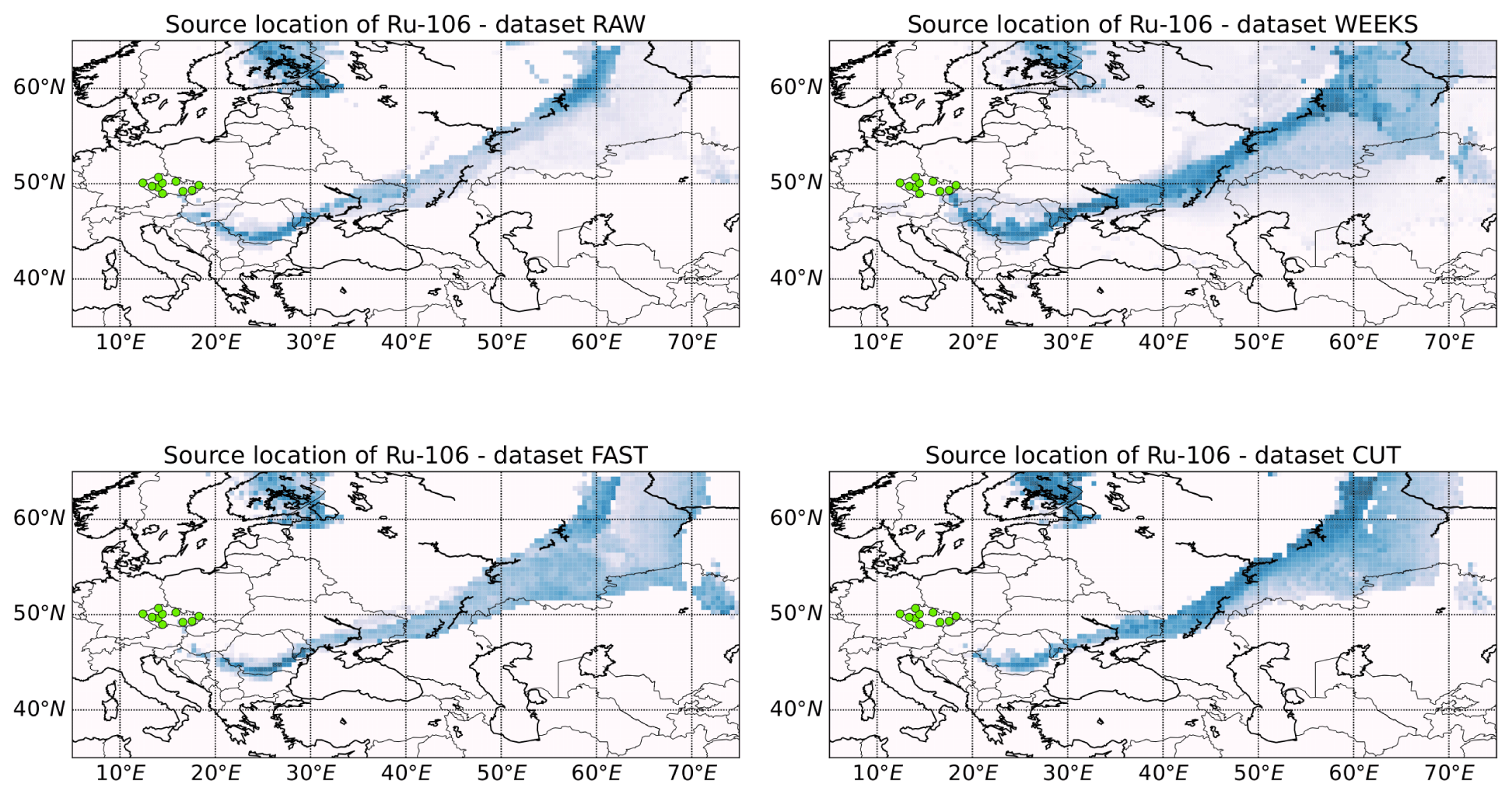
Figure 5Source location of the 106Ru release via the marginal log likelihood, where the observed data are explained by a release from a grid cell using the LS-APC-VB method HYSPLIT atmospheric transport model coupled with GFS 0.5∘ meteorological data. The dataset that has been used is indicated in the titles of each map. The measuring sites are displayed using green dots.
In all four cases, an estimated probability region of source locations forms the strip spanning from southern Romania to approximately the Ob River in the Russian Federation. Notably, these regions are computed on the basis of data from the Czech monitoring stations only. Limited ability of the method to determine one specific location was therefore expected. During the period in question, the wind mostly blew towards the west, which is in agreement with the probable source region located to the east of the Czech Republic. The RAW dataset tends to prefer the northern part of the estimated source location strip, leaving the south part less probable. Similar behavior is observed in the case of the WEEKS dataset, where, in addition, low probability was also observed in wide areas in the south and north of the strip. This is probably caused by the lower temporal resolution of the measurements, implying a wider possibility of radionuclide transport. The results obtained using the FAST and CUT datasets are more homogeneous, covering the whole strip. However, the CUT dataset provides locations with very low probability inside the strip. These are probably artifacts caused by the artificial adjustment of the data. Note that better source location is possible with better spatial distribution of the measuring sites. This is, indeed, available and will be discussed in Sect. 4.3 on the IAEA dataset.
Kovalets and Romanenko (2017)Sørensen (2018)De Meutter et al. (2020)Maffezzoli et al. (2019)Shershakov et al. (2019)Saunier et al. (2019)Le Brazidec et al. (2020)Western et al. (2020)Table 2This table summarizes and compares previous studies on the 106Ru release in 2017, focusing on the total release, the source location, and the temporal character. The last row contains results based on the Czech FAST dataset.
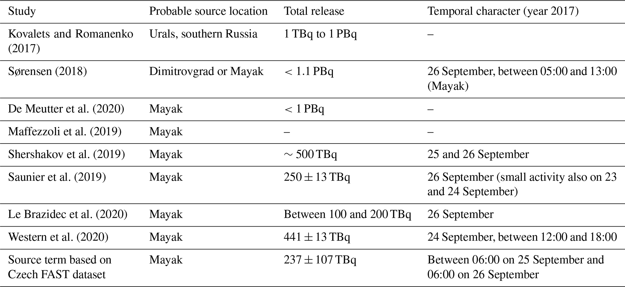
Based on Fig. 5 and a review of the situation in the literature (see Table 2), we consider four source locations. Two of them are Russian nuclear facilities capable of producing a significant amount of 106Ru (Saunier et al., 2019; Masson et al., 2019; Sørensen, 2018): the Research Institute of Atomic Reactors (RIAR) in Dimitrovgrad (location 1) and the Mayak Production Association, a spent fuel reprocessing facility in Ozersk (location 2); see Fig. 6. Location 3 is selected as a location with high probability in all four datasets and is situated to the east of Perm, to the north of the Mayak location. Location 4 is situated in southern Romania and is also a candidate according to all datasets. We are aware that, according to further analyses (Le Brazidec et al., 2020; Saunier et al., 2019; Shershakov et al., 2019; De Meutter et al., 2020; Western et al., 2020), all locations except Mayak, location 2, could be rejected. However, we have considered them here, since they are candidate locations based on just Czech monitoring data. Dimitrovgrad, location 1, was later rejected due to inconsistency with the concentration measurements to the south and east of Dimitrovgrad (Saunier et al., 2019; Maffezzoli et al., 2019). Location 3 is hypothetical, with no known nuclear facility around the location capable of producing a substantial amount of 106Ru that would explain the concentration measurements thousands of kilometers away from this location. A release at location 4 in southern Romania would contradict ground-based observations to the east of the location and was thus also rejected (see Masson et al., 2019). Nevertheless, we will discuss all four possible source terms in these locations in this section, in order to demonstrate the effects of the fast measuring systems.
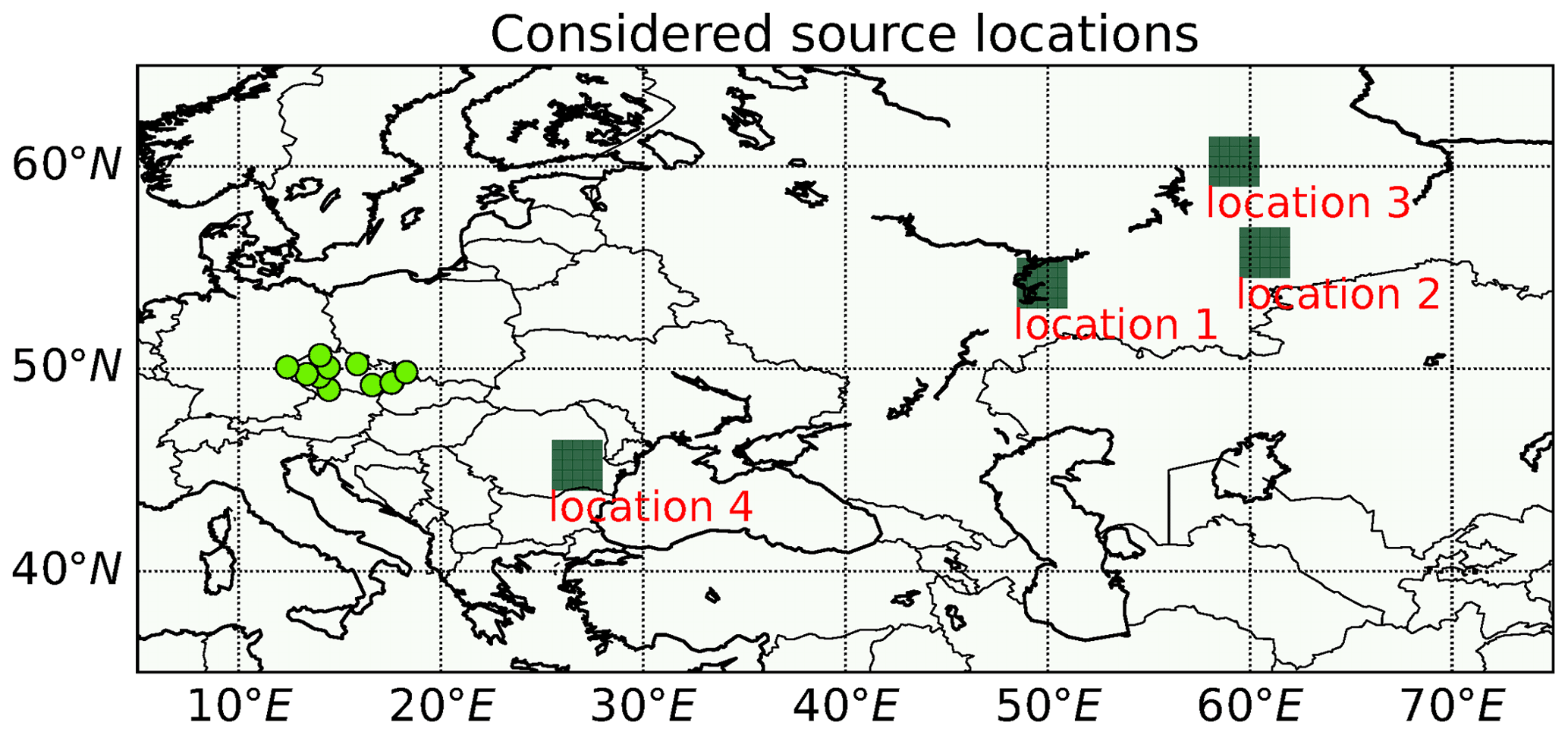
Figure 6The four considered locations are displayed using green squares and labels. The measuring sites are displayed using green dots.

Figure 7Estimated source terms from the locations considered in Fig. 6 (indicated in the titles of each column) for the RAW (blue lines), WEEKS (magenta lines), FAST (red lines), and CUT (green lines) datasets. The estimated source terms are accompanied by the 95 % uncertainty regions (gray-filled regions). Note that the vertical axis has a different scales for each location.
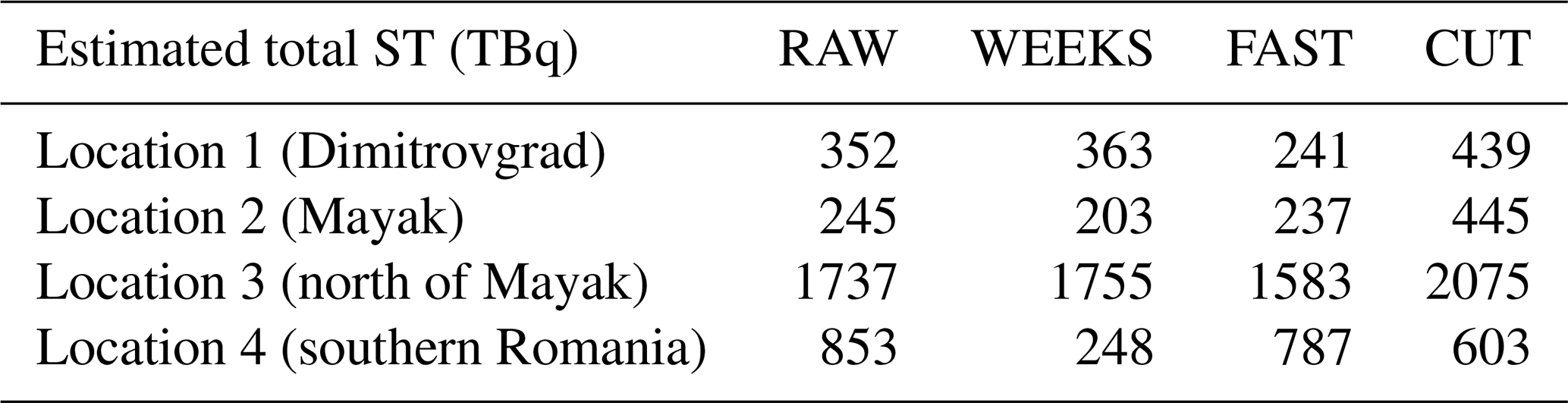
The estimated source terms are displayed in Fig. 7 for all the considered datasets and locations; see the titles and labels. Note that in Fig. 7 we have cropped zero activities at the beginning and at the end of the source terms to maintain better visibility. All source terms are associated with the 95 % (2σ) highest posterior density region, using gray-filled regions. The total estimated activities are further summarized in Table 3. Note that only the Dimitrovgrad and Mayak locations are in agreement with the previously reported total activities of approximately 100–500 TBq (Shershakov et al., 2019; Saunier et al., 2019; Le Brazidec et al., 2020; Western et al., 2020). Estimates from all datasets for these locations fit this interval.
Table 3Estimated total source terms in TBq for a specific dataset (columns) and for a specific location (rows). ST: source term.
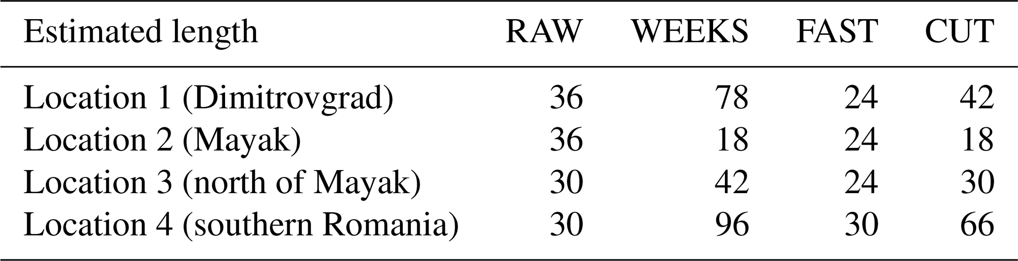
As regards the temporal specification of the release, the estimated lengths of the release are displayed in Table 4. The release probably occurred at Mayak between 25 and 26 September; see the literature review in Table 2. Shershakov et al. (2019) estimated the 2 d interval (both 25 and 26 September), while further analyses by Saunier et al. (2019) and by Le Brazidec et al. (2020) indicate a higher probability of the release on 26 September, with a possible minor release on 23 and 24 September (Saunier et al., 2019). This is consistent with our findings, where 26 September was estimated using the WEEKS and CUT datasets; most of 25 and 26 September was estimated using the RAW dataset; and the time period between 06:00 on 25 September and 06:00 on 26 September was estimated by the FAST dataset. Further validation with the IAEA dataset, Sect. 4.3, shows that the estimates from the WEEKS and FAST datasets are in better agreement with the IAEA-reported concentration measurements than the estimates from the RAW and CUT datasets. Considering that the bulk of the release was probably within 1 d, we conclude that the FAST dataset provides the most consistent results, estimating a 1 d (24 h) release for locations 1, 2, and 3 and 30 h for location 4. The RAW dataset estimated that the release lasted between 30 and 36 h. Wider ranges were obtained in the case of the WEEKS dataset (between 18 and 96 h) and the CUT dataset (between 18 and 66 h). This wide ranges of the release from different locations are probably caused by the natural assumption of the LS-APC model that the shorter release is more probable than a longer one using selection of a zero prior mean value of the source term in Eq. (6). These findings support the hypothesis that the fast measuring systems have better time specificity than the standard measurement procedure.
Table 4Estimated length of non-zero activity (higher than 1 TBq in a period of 6 h) of source terms in hours for a specific dataset (columns) and for a specific location (rows).
4.3 Validation and comparison with the IAEA dataset
The same atmospheric transport modeling procedure as in Sect. 4.1 is applied here to the dataset of the 106Ru measurements available from the IAEA report (IAEA, 2017). This consists of 451 relevant measurements, mostly from northern, eastern, and central Europe and the Russian Federation; see Fig. 10 for the exact locations of the measuring sites. This dataset will serve as a validation set (Czech monitoring data have been removed).
First, scatterplots between the measured data reported by the IAEA and a reconstruction using estimated source terms from the four studied Czech datasets studied here are displayed in Fig. 8 for location 2, Mayak. Here, the same colors as in Fig. 7 for each dataset are used. The scatterplots are accompanied by the computed correlation coefficients (R value) and correlation coefficients of the logarithm of concentrations (Rlog value) given in the legend of each plot. We observed that the highest correlations coefficients are for the WEEKS (0.383) and FAST (0.381) datasets. The RAW dataset has a lower correlation coefficient (0.378), and the CUT dataset has a significantly lower correlation coefficient (0.345). Similar results are obtained also for correlation coefficients of the logarithm of concentrations. This demonstrates that the fast measuring systems provide comparable or even better results than the standard measurement procedure. The artificially constructed CUT dataset has a significantly lower agreement with the IAEA dataset, which may indicate, e.g., inaccuracy in cutting the time intervals of the measurements in this dataset.
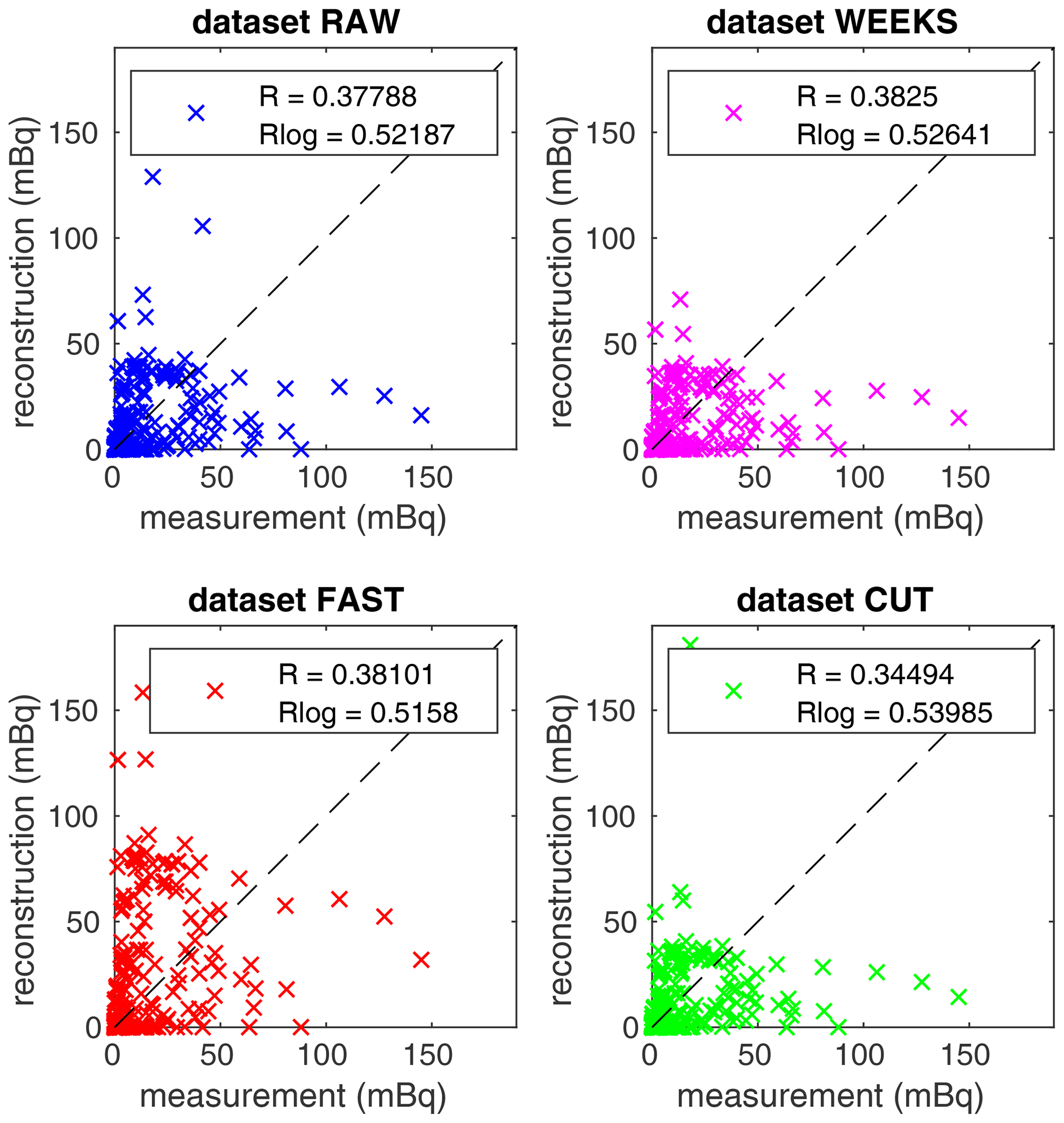
Figure 8Scatterplots between the IAEA measurements and reconstructions using the RAW, WEEKS, FAST, and CUT datasets (specified in titles) for location 2, Mayak. Computed correlation coefficients and correlation coefficients of the logarithm of concentrations are given in the legends.
Second, the scatterplots between the measured data reported by the IAEA and the reconstruction using the FAST dataset for all four considered locations are displayed in Fig. 9, accompanied by the computed correlation coefficients and correlation coefficients of the logarithm of concentrations. Here, the reconstruction for location 2 (Mayak) is in better agreement with the IAEA data than any other considered location. Note that similar results are also obtained for all other datasets, indicating that the Mayak location is the most consistent with the IAEA dataset. This confirms the findings of previous studies (Saunier et al., 2019; Maffezzoli et al., 2019; De Meutter et al., 2018; Le Brazidec et al., 2020), which suggest the Mayak location as the most probable.
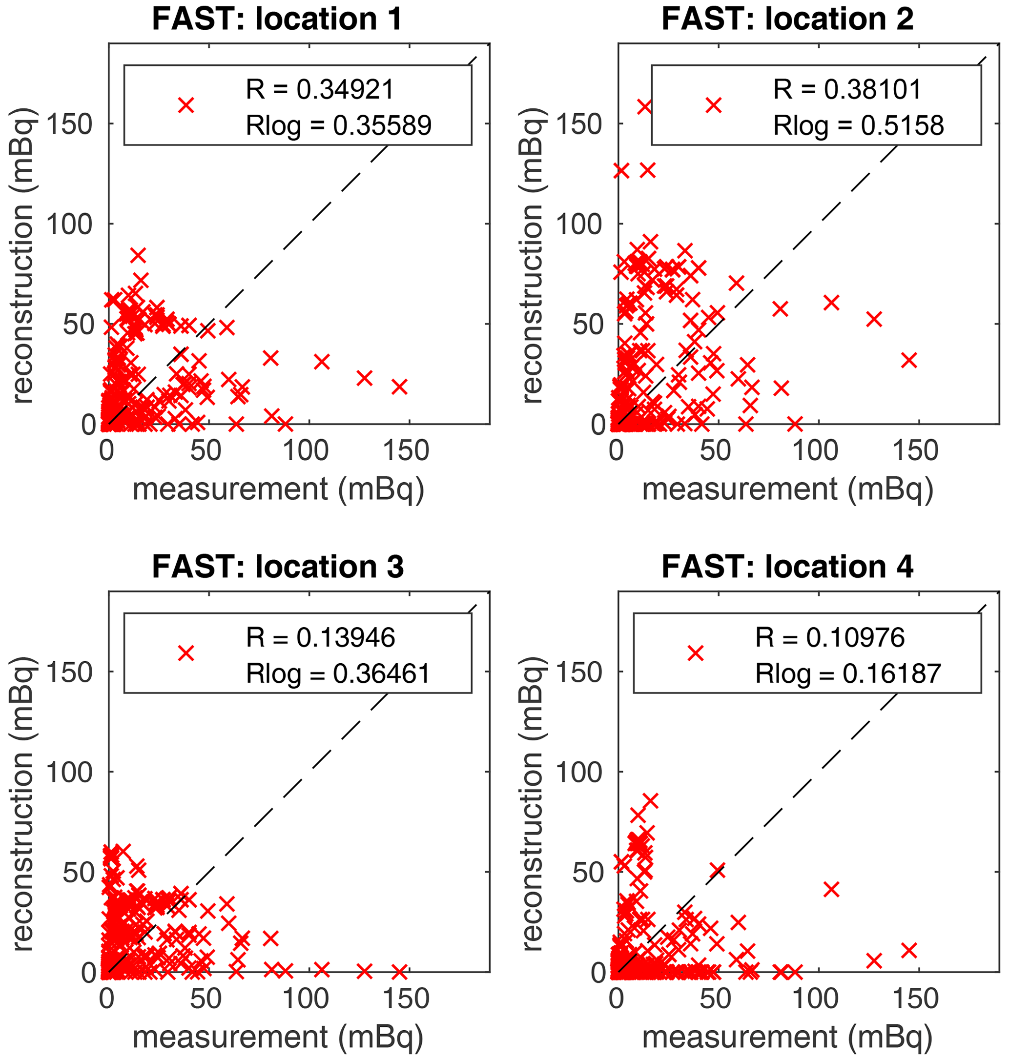
Figure 9Scatterplots between the IAEA measurements and reconstructions using the FAST dataset for all four considered locations (specified in the titles). Computed correlation coefficients and correlation coefficients of the logarithm of concentrations are given in the legends.
Third, as for the Czech monitoring data, the source location methodology from Sect. 3.3 is also applied to the IAEA dataset. The results are displayed in Fig. 10. Again, a darker color denotes a more likely location of the release, while the scale is relative and dimensionless due to the proportional equality in Eq. (11). In direct comparison with the source locations using the smaller datasets studied in Fig. 5, the patterns are very similar. Indeed, the source location using the IAEA dataset rejected locations that cannot be rejected on the basis of the Czech data alone, due to the lack of data; see, e.g., the locations in Romania, Ukraine, and Finland. However, the estimates using all datasets in the southern Urals are consistent with the IAEA dataset results and also with, e.g., the results of Saunier et al. (2019). For a numeric comparison of the source location maps using the Czech datasets and the map using the IAEA dataset, we compute four statistical coefficients used for evaluations of atmospheric modeling results. Concretely, we compute the normalized mean square error (NMSE) which may be, however, biased (Poli and Cirillo, 1993). Therefore, we also compute the normalized mean square error of the distribution of the normalized ratios (NNR) suggested by Poli and Cirillo (1993) accompanied also by the figure of merit in space (FMS) (Abida and Bocquet, 2009) and the fractional bias (FB) (Chang and Hanna, 2004). Note that coefficients closer to zeros are better in all cases except the FMS, where higher is better. These statistical coefficients are defined as
where q is the number of map tiles, pIAEA is the vector with the probabilities of the source location computed using the IAEA dataset, and pset is the vector with the probabilities of the source location computed using the selected Czech dataset. The results are summarized in Fig. 10, below the probability map.
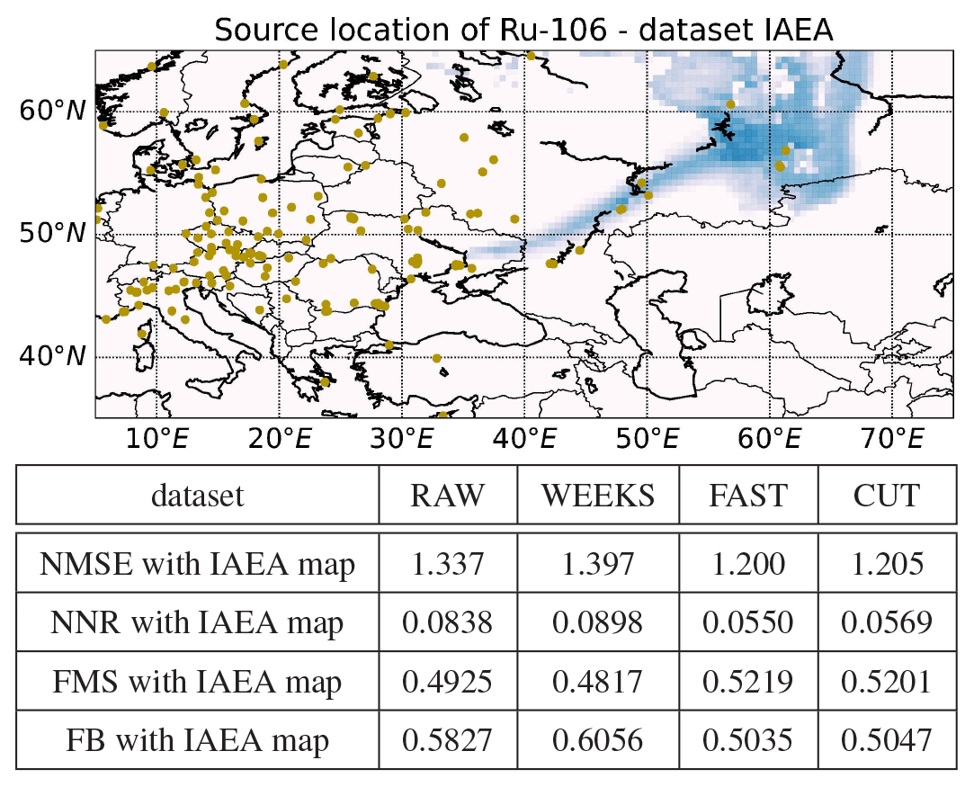
Figure 10Top: source location of the release of 106Ru via marginal log likelihood, using the IAEA dataset. Bottom: the computed normalized mean square error (NMSE), the normalized mean square error of the distribution of the normalized ratios (NNR), the figure of merit in space (FMS), and the fractional bias (FB) between the source location results obtained using the IAEA dataset and the RAW, WEEKS, FAST, and CUT datasets.
We conclude that in all cases, results obtained using the FAST dataset are better than those obtained using other datasets. The CUT dataset performs slightly worse than the FAST dataset, while results obtained using RAW and WEEKS datasets are significantly worse than obtained using FAST and CUT datasets. This demonstrates that the use of fast measurement systems could better reflect the variability of the release even when it is located far from the release site and could better match the results of the IAEA dataset, which has a far better spatial distribution of the measurement stations.
4.4 Results using the FLEXPART model
In this section, we aim to demonstrate that a better time resolution of measurement is beneficial independently on the used atmospheric transport model and the used time-resolution. Concretely, we use the FLEXPART model (Pisso et al., 2019) in backward mode with a finer, 3 h output temporal resolution as described in Sect. 4.1.
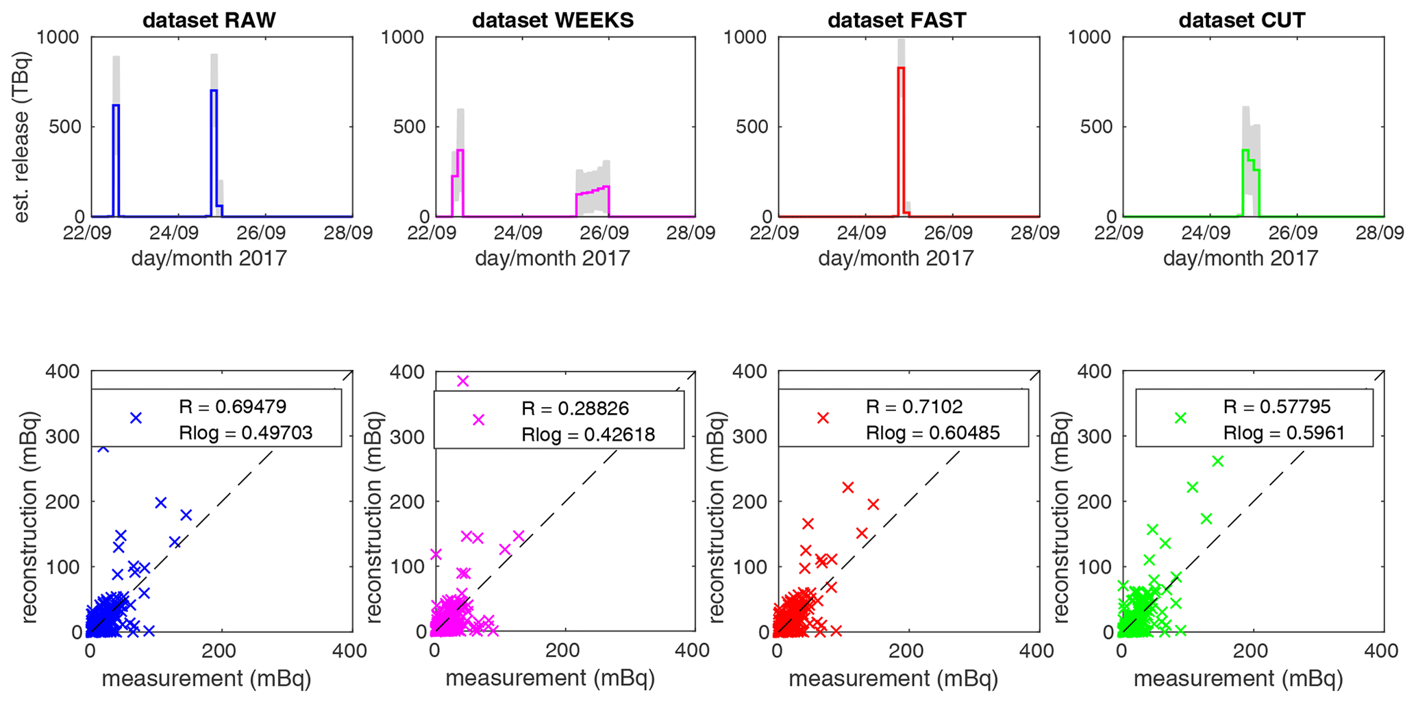
Figure 11Estimated (est.) source terms for location 2, Mayak, using SRS matrices computed using the FLEXPART atmospheric transport model (top row) associated with scatterplots between the IAEA-reported measurements and reconstruction using specified dataset (bottom row). The coloring of panels is the same as in Figs. 7 and 8.
We present results for considered location 2, Mayak, in Fig. 11. There are source terms estimated using the LS-APC algorithm in the top row and a scatterplot between measured data reported by the IAEA and a reconstruction using each dataset in the bottom row. Note that the coloring of panels is the same as in Figs. 7 and 8. The totals of the source terms are 1388, 1459, 852, and 948 TBq for datasets RAW, WEEKS, FAST, and CUT respectively. The lengths of releases are 18, 24, 9, and 12 h for datasets RAW, WEEKS, FAST, and CUT respectively.
The following differences are observed in comparison with results based on HYSPLIT runs. First, we observe significant releases between 22 and 23 September in the case of the RAW and WEEKS datasets. These releases are not observed for the FAST and CUT datasets. However, note also that the response on this initial release in, e.g., the IAEA dataset is relatively low; see the comparison of R values in Fig. 11. Second, the release periods are estimated in the beginning of 25 September rather than in the end as in the case of the HYSPLIT runs; however, this difference is negligible considering the spatiotemporal domain. Third, totals of releases are in all cases significantly larger than in the case of the HYSPLIT runs. The reason for this disproportion may be in the different parametrization of the atmospheric model. Considering the scatterplots on the bottom of Fig. 11, we assume the estimated releases are slightly overestimated, while they are on the upper limit of estimates in the literature as in Table 2.
From this perspective, the better temporal resolution of the output temporal grid seems to better reflect the better temporal resolution of the measurements. Similarly to Sect. 4.3, we also validate (with the use of FLEXPART) the estimated source terms with the IAEA-reported measurements and compute the associated R value for each scatterplot in Fig. 11. The R value is slightly better for the FAST dataset (0.710) than for the RAW dataset (0.695), while it is 0.578 for the RAW dataset and even lower for the WEEKS dataset (0.288). These results support the hypothesis that better temporal resolution of measurements is beneficial for source term inversion.
We have investigated the occurrence of 106Ru in Europe in the fall of 2017. We have used data from the Czech Radiation Monitoring Network, which also includes measurement data from novel real-time monitoring systems. Based on this case study, it can be concluded that both systems are suitable for the task of rapid detection of radioactive contamination in the atmosphere at the level of mBq m−3. Each of the developed devices employs a different sampling–measurement procedure, and therefore there are also different possibilities for their integration into a large-scale monitoring network. The combination of the AMARA system and laboratory measurement seems to be an optimal setup, balancing response sensitivity and timeliness. On the other hand, the CEGAM system can be operated unattended in remote locations in a standby regime with a relatively low power consumption and can be switched to an emergency regime if needed. Regarding the employed electrically cooled HPGe detectors, they proved to be resilient enough to be deployed long term. For the past 3 years we have not experienced any malfunction or need of excessive maintenance, so the only drawback of HPGe detectors is the accompanied costs compared to the NaI (Tl) setup which we used in the past.
Using the inversion modeling technique, we have compared the results obtained from four datasets ranging from raw data, using the standard measuring procedure, to real-time monitoring data with a much better temporal resolution. The results have been compared with the published state-of-the-art estimates of the 106Ru release in 2017. Based on this comparison, we have observed that the results obtained using real-time monitoring data are comparable in terms of the total estimated release and are better for the temporal specification of the release, and they are consistent with the previously reported findings regarding the location of the 106Ru source term.
In addition, we have compared our results based on the Czech monitoring data with the dataset reported by the IAEA, which has a much better spatial coverage. The source location results have been compared using the NMSE, NNR, FMS, and FB coefficients between the IAEA results and the results based on the Czech monitoring data. We have concluded that the real-time monitoring data result is close to the IAEA result. Four source location hypotheses have been tested based on the correlation coefficient between the IAEA measurements and the model reconstruction using Czech monitoring data. Here, the results are in agreement with previous studies, with the Mayak location being the most probable (R=0.381) in comparison with Dimitrovgrad (R=0.349), southern Romania (R=0.139), and the location to the north of Mayak (R=0.109).
Concerning the real-time monitoring capabilities of the Czech Radiation Monitoring Network, we have shown that a single operating device can enhance the inverse modeling predictions even for a relatively low radionuclide concentration at the level of mBq m−3. Although the continental-scale scenario such as the 106Ru case in 2017 may not be ideal for quantification of a real-time monitoring system due to the diffusion over several days of transport, we believe that the benefits are still observable. It is safe to state that the installation of multiple devices such as AMARA and CEGAM over a larger region (on a European scale) would certainly yield additional improvements in source location and in source term estimation in the event of a radionuclide atmospheric release.
The Czech datasets are freely available as the Supplement of this paper. The HYSPLIT and FLEXPART models are open source and are freely available from their developers. Reference MATLAB implementations of algorithms can be obtained from the corresponding author upon request.
The supplement related to this article is available online at: https://doi.org/10.5194/amt-14-803-2021-supplement.
OT designed and performed the experiments and wrote the paper. MH designed experiments, conducted measurements, and wrote the paper. NE performed FLEXPART simulations and commented on the paper. VS commented on the paper and inversion procedure.
The authors declare that they have no conflict of interest.
This research has been supported by the Czech Science Foundation (grant no. GA20-27939S) and the Ministry of the Interior of the Czech Republic (grant no. VI20152018042).
This paper was edited by Ronald Cohen and reviewed by Daniel Lienhard and one anonymous referee.
Abida, R. and Bocquet, M.: Targeting of observations for accidental atmospheric release monitoring, Atmos. Environ., 43, 6312–6327, 2009. a
ACRO: Note Technique relative à l'incident du 31 octobre 2001 et aux retombées des incidents ruthénium survenus à Cogéma-La Hague en 2001, HEROUVILLE ST CLAIR, Report Number INIS-FR-08-1453, 17 pp., available at: https://inis.iaea.org/search/search.aspx?orig_q=RN:40007585 (last access: 25 May 2020), 2002 (in French). a
Berchet, A., Pison, I., Chevallier, F., Bousquet, P., Conil, S., Geever, M., Laurila, T., Lavrič, J., Lopez, M., Moncrieff, J., Necki, J., Ramonet, M., Schmidt, M., Steinbacher, M., and Tarniewicz, J.: Towards better error statistics for atmospheric inversions of methane surface fluxes, Atmos. Chem. Phys., 13, 7115–7132, https://doi.org/10.5194/acp-13-7115-2013, 2013. a
Bernardo, J. and Smith, A.: Bayesian theory, vol. 405, John Wiley & Sons, Hoboken, USA, 2009. a
Bishop, C.: Pattern recognition and machine learning, Springer, New York, USA, 2006. a
Bossew, P., Gering, F., Petermann, E., Hamburger, T., Katzlberger, C., Hernandez-Ceballos, M., De Cort, M., Gorzkiewicz, K., Kierepko, R., and Mietelski, J.: An episode of Ru-106 in air over Europe, September–October 2017 – Geographical distribution of inhalation dose over Europe, J. Environ. Radioactiv., 205, 79–92, 2019. a
Brunner, D., Henne, S., Keller, C. A., Reimann, S., Vollmer, M. K., O'Doherty, S., and Maione, M.: An extended Kalman-filter for regional scale inverse emission estimation, Atmos. Chem. Phys., 12, 3455–3478, https://doi.org/10.5194/acp-12-3455-2012, 2012. a
Carlton, W. and Denham, M.: Assessment of selected fission products in the Savannah River Site environment, Tech. rep., Westinghouse Savannah River Co., https://doi.org/10.2172/554138, 1997. a
Cassiani, M., Stohl, A., and Brioude, J.: Lagrangian stochastic modelling of dispersion in the convective boundary layer with skewed turbulence conditions and a vertical density gradient: Formulation and implementation in the FLEXPART model, Bound.-Lay. Meteorol., 154, 367–390, 2015. a
Chang, J. and Hanna, S.: Air quality model performance evaluation, Meteorol. Atmos. Phys., 87, 167–196, 2004. a
Chz, I.: Zpráva o radiační situaci na území ČSSR po havárii jaderné elektrárny Černobyl, Prague Institut hygieny a epidemiologie, Centrum hygieny záření, 1987 (in Czech). a
De Meutter, P. and Hoffman, I.: Bayesian source reconstruction of an anomalous Selenium-75 release at a nuclear research institute, J. Environ. Radioactiv., 218, 106225, https://doi.org/10.1016/j.jenvrad.2020.106225, 2020. a
De Meutter, P., Camps, J., Delcloo, A., and Termonia, P.: Source localisation and its uncertainty quantification after the third DPRK nuclear test, Sci. Rep.-UK, 8, 10155, https://doi.org/10.1038/s41598-018-28403-z, 2018. a, b
De Meutter, P., Camps, J., Delcloo, A., and Termonia, P.: Source Localization of Ruthenium-106 Detections in Autumn 2017 Using Inverse Modelling, in: Air Pollution Modeling and its Application XXVI. ITM 2018, edited by: Mensink, C., Gong, W., and Hakami, A., Springer Proceedings in Complexity, Springer, Cham, https://doi.org/10.1007/978-3-030-22055-6_15, 2020. a, b, c
Draxler, R. and Hess, G.: Description of the HYSPLIT_4 modeling system, NOAA Technical Memorandum ERL ARL-224, Silver Spring, Maryland, USA, 1997. a
Eckhardt, S., Prata, A. J., Seibert, P., Stebel, K., and Stohl, A.: Estimation of the vertical profile of sulfur dioxide injection into the atmosphere by a volcanic eruption using satellite column measurements and inverse transport modeling, Atmos. Chem. Phys., 8, 3881–3897, https://doi.org/10.5194/acp-8-3881-2008, 2008. a
Evangeliou, N., Hamburger, T., Cozic, A., Balkanski, Y., and Stohl, A.: Inverse modeling of the Chernobyl source term using atmospheric concentration and deposition measurements, Atmos. Chem. Phys., 17, 8805–8824, https://doi.org/10.5194/acp-17-8805-2017, 2017. a, b, c
Forster, C., Stohl, A., and Seibert, P.: Parameterization of convective transport in a Lagrangian particle dispersion model and its evaluation, J. Appl. Meteorol. Clim., 46, 403–422, 2007. a
Grythe, H., Kristiansen, N. I., Groot Zwaaftink, C. D., Eckhardt, S., Ström, J., Tunved, P., Krejci, R., and Stohl, A.: A new aerosol wet removal scheme for the Lagrangian particle model FLEXPART v10, Geosci. Model Dev., 10, 1447–1466, https://doi.org/10.5194/gmd-10-1447-2017, 2017. a
Henne, S., Brunner, D., Oney, B., Leuenberger, M., Eugster, W., Bamberger, I., Meinhardt, F., Steinbacher, M., and Emmenegger, L.: Validation of the Swiss methane emission inventory by atmospheric observations and inverse modelling, Atmos. Chem. Phys., 16, 3683–3710, https://doi.org/10.5194/acp-16-3683-2016, 2016. a
Hýža, M. and Rulík, P.: Low-level atmospheric radioactivity measurement using a NaI (Tl) spectrometer during aerosol sampling, Appl. Radiat. Isotopes, 126, 225–227, 2017. a
IAEA: Updated Technical Attachment Status of Measurements of Ru-106 in Europe, Tech. rep., IAEA, Vienna, Austria, 2017. a, b, c
Kovalets, I. and Romanenko, A.: Detection of ruthenium-106 in 2017: meteorological analysis of the potential sources, research report, https://doi.org/10.13140/RG.2.2.36537.67685, 2017. a, b
Kristiansen, N., Stohl, A., Prata, A., Richter, A., Eckhardt, S., Seibert, P., Hoffmann, A., Ritter, C., Bitar, L., Duck, T., and Stebel, K.: Remote sensing and inverse transport modeling of the Kasatochi eruption sulfur dioxide cloud, J. Geophys. Res.-Atmos., 115, 1984–2012, 2010. a
Le Brazidec, J., Bocquet, M., Saunier, O., and Roustan, Y.: MCMC methods applied to the reconstruction of the autumn 2017 Ruthenium-106 atmospheric contamination source, Atmos. Environ., 6, 100071, https://doi.org/10.1016/j.aeaoa.2020.100071, 2020. a, b, c, d, e, f
Liu, Y., Haussaire, J.-M., Bocquet, M., Roustan, Y., Saunier, O., and Mathieu, A.: Uncertainty quantification of pollutant source retrieval: comparison of Bayesian methods with application to the Chernobyl and Fukushima Daiichi accidental releases of radionuclides, Q. J. Roy. Meteor. Soc., 143, 2886–2901, 2017. a
Maffezzoli, N., Baccolo, G., Di Stefano, E., and Clemenza, M.: The Ruthenium-106 plume over Europe in 2017: A source-receptor model to estimate the source region, Atmos. Environ., 212, 239–249, 2019. a, b, c, d
Masson, O., Baeza, A., Bieringer, J., Brudecki, K., Bucci, S., Cappai, M., Carvalho, F. P., Connan, O., Cosma, C., Dalheimer, A., Didier, D., Depuydt, G., De Geer, L. E., De Vismes, A., Gini, L., Groppi, F., Gudnason, K., Gurriaran, R., Hainz, D., Halldórsson, Ó., Hammond, D., Hanley, O., Holeý, K., Homoki, Zs., Ioannidou, A., Isajenko, K., Jankovic, M., Katzlberger, C., Kettunen, M., Kierepko, R., Kontro, R., Kwakman, P. J. M., Lecomte, M., Leon Vintro, L., Leppänen, A.-P., Lind, B., Lujaniene, G., McGinnity, P., Mahon, C. M., Malá, H., Manenti, S., Manolopoulou, M., Mattila, A., Mauring, A., Mietelski, J. W., Møller, B., Nielsen, S. P., Nikolic, J., Overwater, R. M. W., Pálsson, S. E., Papastefanou, C., Penev, I., Pham, M. K., Povinec, P. P., Ramebäck, H., Reis, M. C., Ringer, W., Rodriguez, A., Rulík, P., Saey, P. R. J., Samsonov, V., Schlosser, C., Sgorbati, G., Silobritiene, B. V., Söderström, C., Sogni, R., Solier, L., Sonck, M., Steinhauser, G., Steinkopff, T., Steinmann, P., Stoulos, S., Sýkora, I., Todorovic, D., Tooloutalaie, N., Tositti, L., Tschiersch, J., Ugron, A., Vagena, E., Vargas, A., Wershofen, H., and Zhukova, O.: Tracking of airborne radionuclides from the damaged Fukushima Dai-ichi nuclear reactors by European networks, Environ. Sci. Technol., 45, 7670–7677, 2011. a
Masson, O., Steinhauser, G., Wershofen, H., Mietelski, J. W., Fischer, H. W., Pourcelot, L., Saunier, O., Bieringer, J., Steinkopff, T., Hýža, M., Moller, B., Bowyer, T. W., Dalaka, E., Dalheimer, A., de Vismes-Ott, A., Eleftheriadis, K., Forte, M., Gasco Leonarte, C., Gorzkiewicz, K., Homoki, Z., Isajenko, K., Karhunen, T., Katzlberger, C., Kierepko, R., Kovendiné Kónyi, J., Malá, H., Nikolic, J., Povinec, P. P., Rajacic, M., Ringer, W., Rulík, P., Rusconi, R., Sáfrány, G., Sykora, I., Todorovic, D., Tschiersch, J., Ungar, K., and Zorko, B.: Potential Source Apportionment and Meteorological Conditions Involved in Airborne 131I Detections in January/February 2017 in Europe, Environ. Sci. Technol., 52, 8488–8500, 2018. a
Masson, O., Steinhauser, G., Zok, D., Saunier, O., Angelov, H., Babić, D., Bečková, V., Bieringer, J., Bruggeman, M., Burbidge, C. I., Conil, S., Dalheimer, A., De Geer, L.-E., de Vismes Ott, A., Eleftheriadis, K., Estier, S., Fischer, H., Garavaglia, M. G., Gasco Leonarte, C., Gorzkiewicz, K., Hainz, D., Hoffman, I., Hýža, M., Isajenko, K., Karhunen, T., Kastlander, J., Katzlberger, C., Kierepko, R., Knetsch, G.-J., Kövendiné Kónyi, J., Lecomte, M., Mietelski, J. W., Min, P., Møller, B., Nielsen, S. P., Nikolic, J., Nikolovska, L., Penev, I., Petrinec, B., Povinec, P. P., Querfeld, R., Raimondi, O., Ransby, D., Ringer, W., Romanenko, O., Rusconi, R., Saey, P. R. J., Samsonov, V., Šilobritiene, B., Simion, E., Söderström, C.,Šoštarić, M., Steinkopff, T., Steinmann, P., Sýkora, I., Tabachnyi, L., Todorovic, D., Tomankiewicz, E., Tschiersch, J., Tsibranski, R., Tzortzis, M., Ungar, K., Vidic, A., Weller, A., Wershofen, H., Zagyvai, P., Zalewska, T., and Zapata García, D. and Zorko, B.: Airborne concentrations and chemical considerations of radioactive ruthenium from an undeclared major nuclear release in 2017, P. Natl. Acad. Sci., 116, 16750–16759, 2019. a, b, c, d, e
Minty, B. and Hovgaard, J.: Reducing noise in gamma-ray spectrometry using spectral component analysis, Explor. Geophys., 33, 172–176, 2002. a
Nikitina, O. and Slobodenyuk, I.: The French Newspaper Le Figaro Claims That a Possible Source of Emissions of Ruthenium Could Be Russian Mayak, Tech. rep., IBRAE, available at: http://en.ibrae.ac.ru/newstext/889/ (last access: 25 May 2020), 2018. a
Nisbet, E. and Weiss, R.: Top-down versus bottom-up, Science, 328, 1241–1243, 2010. a
Pisso, I., Sollum, E., Grythe, H., Kristiansen, N. I., Cassiani, M., Eckhardt, S., Arnold, D., Morton, D., Thompson, R. L., Groot Zwaaftink, C. D., Evangeliou, N., Sodemann, H., Haimberger, L., Henne, S., Brunner, D., Burkhart, J. F., Fouilloux, A., Brioude, J., Philipp, A., Seibert, P., and Stohl, A.: The Lagrangian particle dispersion model FLEXPART version 10.4, Geosci. Model Dev., 12, 4955–4997, https://doi.org/10.5194/gmd-12-4955-2019, 2019. a, b, c
Poli, A. A. and Cirillo, M.: On the use of the normalized mean square error in evaluating dispersion model performance, Atmos. Environ., 27, 2427–2434, 1993. a, b
Saunier, O., Didier, D., Mathieu, A., Masson, O., and Le Brazidec, J.: Atmospheric modeling and source reconstruction of radioactive ruthenium from an undeclared major release in 2017, P. Natl. Acad. Sci., 116, 24991–25000, 2019. a, b, c, d, e, f, g, h, i, j, k
Seibert, P.: Iverse modelling with a Lagrangian particle disperion model: application to point releases over limited time intervals, in: Air Pollution Modeling and Its Application XIV, edited by: Gryning, S. E. and Schiermeier, F. A., Springer, Boston, MA, USA, 381–389, https://doi.org/10.1007/0-306-47460-3_38, 2001. a
Seibert, P. and Frank, A.: Source-receptor matrix calculation with a Lagrangian particle dispersion model in backward mode, Atmos. Chem. Phys., 4, 51–63, https://doi.org/10.5194/acp-4-51-2004, 2004. a
Shershakov, V., Borodin, R., and Tsaturov, Y.: Assessment of Possible Location Ru-106 Source in Russia in September–October 2017, Russ. Meteorol. Hydrol., 44, 196–202, 2019. a, b, c, d, e
Šmídl, V. and Quinn, A.: The Variational Bayes Method in Signal Processing, Springer, Berlin, Heidelberg, Germany, 2006. a
Song, S., Selin, N. E., Soerensen, A. L., Angot, H., Artz, R., Brooks, S., Brunke, E.-G., Conley, G., Dommergue, A., Ebinghaus, R., Holsen, T. M., Jaffe, D. A., Kang, S., Kelley, P., Luke, W. T., Magand, O., Marumoto, K., Pfaffhuber, K. A., Ren, X., Sheu, G.-R., Slemr, F., Warneke, T., Weigelt, A., Weiss-Penzias, P., Wip, D. C., and Zhang, Q.: Top-down constraints on atmospheric mercury emissions and implications for global biogeochemical cycling, Atmos. Chem. Phys., 15, 7103–7125, https://doi.org/10.5194/acp-15-7103-2015, 2015. a
Sørensen, J.: Method for source localization proposed and applied to the October 2017 case of atmospheric dispersion of Ru-106, J. Environ. Radioactiv., 189, 221–226, 2018. a, b
Stein, A., Draxler, R., Rolph, G., Stunder, B., Cohen, M., and Ngan, F.: NOAA's HYSPLIT atmospheric transport and dispersion modeling system, B. Am. Meteorol. Soc., 96, 2059–2077, 2015. a
Stohl, A., Forster, C., Frank, A., Seibert, P., and Wotawa, G.: Technical note: The Lagrangian particle dispersion model FLEXPART version 6.2, Atmos. Chem. Phys., 5, 2461–2474, https://doi.org/10.5194/acp-5-2461-2005, 2005. a
Stohl, A., Seibert, P., Arduini, J., Eckhardt, S., Fraser, P., Greally, B. R., Lunder, C., Maione, M., Mühle, J., O'Doherty, S., Prinn, R. G., Reimann, S., Saito, T., Schmidbauer, N., Simmonds, P. G., Vollmer, M. K., Weiss, R. F., and Yokouchi, Y.: An analytical inversion method for determining regional and global emissions of greenhouse gases: Sensitivity studies and application to halocarbons, Atmos. Chem. Phys., 9, 1597–1620, https://doi.org/10.5194/acp-9-1597-2009, 2009. a
Stohl, A., Seibert, P., Wotawa, G., Arnold, D., Burkhart, J. F., Eckhardt, S., Tapia, C., Vargas, A., and Yasunari, T. J.: Xenon-133 and caesium-137 releases into the atmosphere from the Fukushima Dai-ichi nuclear power plant: determination of the source term, atmospheric dispersion, and deposition, Atmos. Chem. Phys., 12, 2313–2343, https://doi.org/10.5194/acp-12-2313-2012, 2012. a, b
Takiar, V., Voong, K., Gombos, D., Mourtada, F., Rechner, L., Lawyer, A., Morrison, W., Garden, A., and Beadle, B.: A choice of radionuclide: Comparative outcomes and toxicity of ruthenium-106 and iodine-125 in the definitive treatment of uveal melanoma, Practical Radiation Oncology, 5, 169–176, 2015. a
Tcherkezian, V., Galushkin, B., Goryachenkova, T., Kashkarov, L., Liul, A., Roschina, I., and Rumiantsev, O.: Forms of contamination of the environment by radionuclides after the Tomsk accident (Russia, 1993), J. Environ. Radioactiv., 27, 133–139, 1995. a
Tichý, O., Šmídl, V., Hofman, R., and Stohl, A.: LS-APC v1.0: a tuning-free method for the linear inverse problem and its application to source-term determination, Geosci. Model Dev., 9, 4297–4311, https://doi.org/10.5194/gmd-9-4297-2016, 2016. a, b, c, d, e, f, g, h
Tichý, O., Šmídl, V., Hofman, R., Šindelářová, K., Hýža, M., and Stohl, A.: Bayesian inverse modeling and source location of an unintended 131I release in Europe in the fall of 2011, Atmos. Chem. Phys., 17, 12677–12696, https://doi.org/10.5194/acp-17-12677-2017, 2017. a, b, c, d, e
Tichý, O., Ulrych, L., Šmídl, V., Evangeliou, N., and Stohl, A.: On the tuning of atmospheric inverse methods: comparisons with the European Tracer Experiment (ETEX) and Chernobyl datasets using the atmospheric transport model FLEXPART, Geosci. Model Dev., 13, 5917–5934, https://doi.org/10.5194/gmd-13-5917-2020, 2020. a
Tipping, M. and Bishop, C.: Probabilistic principal component analysis, J. R. Stat. Soc., 61, 611–622, 1999. a
UNSCEAR: Sources and effects of ionizing radiation: sources, United Nations Publications, New York, USA, 2000. a
Western, L., Millington, S., Benfield-Dexter, A., and Witham, C.: Source estimation of an unexpected release of Ruthenium-106 in 2017 using an inverse modelling approach, J. Environ. Radioactiv., 220, 106304, https://doi.org/10.1016/j.jenvrad.2020.106304, 2020. a, b, c, d