Quantifying fugitive gas emissions from an oil sands tailings pond with open-path Fourier transform infrared measurements

Fugitive emissions from tailings ponds contribute significantly to facility emissions in the Alberta oil sands, but details on chemical emission profiles and the temporal and spatial variability of emissions to the atmosphere are sparse, since flux measurement techniques applied for compliance monitoring have their limitations. In this study, open-path Fourier transform infrared spectroscopy was evaluated as a potential alternative method for quantifying spatially representative fluxes for various pollutants (methane, ammonia, and alkanes) from a particular pond, using vertical-flux-gradient and inverse-dispersion methods. Gradient fluxes of methane averaged 4.3 g m⁻² d⁻¹ but were 44 % lower than nearby eddy covariance measurements, while inverse-dispersion fluxes agreed to within 30 %. With the gradient fluxes method, significant NH₃ emission fluxes were observed (0.05 g m⁻² d⁻¹, 42 t yr⁻¹), and total alkane fluxes were estimated to be 1.05 g m⁻² d⁻¹ (881 t yr⁻¹), representing 9.6 % of the facility emissions.

1 Introduction

Tailings from the oil sands industrial processes in Alberta's Athabasca oil sands consist of a mixture of water, sand, non-recovered bitumen, and additives from the bitumen extraction processes (Small et al., 2015). These tailings are deposited into large engineered tailings ponds on site. Separation of processed water from remaining tailings occurs continuously in the tailings pond, and the processed water is recycled (Canada's oil sands tailings ponds: https://www.canadasoilsands.ca/en/explore-topics/tailings-ponds, last access: 29 September 2019). The total liquid surface area covered by tailings ponds in the Athabasca oil sands was 103 km² in 2016 and continues to grow (Alberta Environment and Parks, 2016).

Emissions to the atmosphere from tailings ponds include methane (CH₄), carbon dioxide (CO₂), reduced sulfur compounds, volatile organic compounds (VOCs), and polycyclic aromatic hydrocarbons (PAHs) (Siddique et al., 2007; Simpson et al., 2010; Yeh et al., 2010; Siddique et al., 2011, 2012; Galarneau et al., 2014; Small et al., 2015; Bari and Kindzierski, 2018; Zhang et al., 2019; Foght et al., 2017; Penner and Foght, 2010). Emissions from tailings ponds vary with pond conditions, such as pond age and solvent additives in the ponds, and can contribute significantly to total facility emissions (Small et al., 2015).

Very few studies focusing on emissions of air pollutants from tailings ponds have been published (Galarneau et al., 2014; Small et al., 2015; Zhang et al., 2019). Compounds of particular interest include alkanes and ammonia (NH₃). Alkanes are part of the solvents used in the extraction process (Small et al., 2015) and can dominate VOCs emissions from oil sands facilities (Li et al., 2017). Previously reported VOCs emissions by facilities had large uncertainties, especially from fugitive sources, due to limitations of the methods used to estimate emissions for compliance monitoring purposes (Li et al., 2017). VOCs in the atmosphere are important because of their effects on ambient ozone and secondary aerosol formation (Field et al., 2015; Kroll and Seinfeld, 2008). Emissions of NH₃ from tailings ponds to the atmosphere have not been published, although NH₃ has been observed in the oil sands region (Bytnerowicz et al., 2010; Whaley et al., 2018). NH₃ emissions have important environmental implications, such as forming atmospheric aerosols with sulfuric acid (Kürten, et al., 2016) and affecting nitrogen deposition in the ecosystem (Makar, et al., 2018). This information is important for model simulations of critical loads of acidifying deposition in the ecosystem (Makar, et al., 2018). This field measurement project provided a great opportunity to continuously measure and to quantify tailings pond emissions over more than a month, especially for NH₃ and total alkanes.

Open-path Fourier transform infrared (OP-FTIR) spectroscopy has been considered a good candidate for an alternative method to monitor fugitive emissions from industrial or hazardous waste area sources, since the method is non-intrusive, integrates over long path lengths, and has the ability to quantify several different gases of interest simultaneously and continuously (Marshall et al., 1994), without sample line issues. It has previously been used to quantify mole fractions of various air pollutants from different sources such as forest fires (Griffith et al., 1991; Yokelson et al., 1996, 1997; Goode et al., 1999; Yokelson, 1999; Yokelson et al., 2007; Burling et al., 2010; Johnson et al., 2010; Akagi et al., 2013; Yokelson et al., 2013; Akagi et al., 2014; Paton-Walsh et al., 2014; Smith et al., 2014), volcanoes (Horrocks et al., 1999; Oppenheimer and Kyle, 2008), industrial sites (Wu et al., 1995), harbors (Wiacek et al., 2018), and road vehicles (Bradley et al., 2000; Grutter et al., 2003; You et al., 2017). OP-FTIR measurements with vertically separated paths have previously been conducted to derive the emission rate of air pollutants. Schäfer et al. (2012) deployed two OP-FTIR spectrometers with parallel paths 2.2 m vertically apart at a grassland in Fuhrberg, Germany, to measure nitrous oxide (N₂O) emissions with a flux-gradient method and showed the calculated flux is comparable to the chamber measurements at the same grassland. Flesch et al. (2016) deployed OP-FTIR measurement with one spectrometer and two paths vertically separated by about 1 m on average (slant path configuration) at a cattle field in Alberta, Canada. They derived emission rates of N₂O and NH₃ by flux-gradient and inverse-dispersion methods, demonstrating the capability of OP-FTIR systems to measure emission rates of N₂O and NH₃. Following the flux-gradient method in Flesch et al. (2016), Bai et al. (2018) measured the flux of N₂O, NH₃, CH₄, and CO₂ from a vegetable farm in Australia using an OP-FTIR system with two paths vertically separated by 0.5 m on average. At the same vegetable farm, Bai et al. (2019) measured emission rates of N₂O using flux chambers and OP-FTIR slant path configuration with flux-gradient methods and showed a large variation of the ratio of N₂O fluxes with these two measurements. Inverse-dispersion models have also been applied to OP-FTIR measurements to quantify emission rates in previous studies (Flesch et al., 2004, 2005; Bai et al., 2014; Hu et al., 2016; Shonkwiler and Ham, 2018).

Longer continuous coverage with a greater height difference between paths is one distinguishing feature of this study compared to previous research. The motivation of this work is to quantify emission rates of pollutants from one specific tailings pond by combining OP-FTIR measurements with micrometeorological methods. Emissions of CH₄, NH₃, and total alkanes as well as a comparison of gradient and inverse-dispersion methods are presented in this study.

2 Open-path FTIR field measurements and methods for deriving fluxes

2.1 Site and measurement setup

The main site of this study was on the south shore of Suncor Pond 2/3 (Fig. 1; 56^∘59^′0.90^′′ N, 111^∘30^′30.30^′′ W, 305 m a.s.l.). Sensible heat and momentum fluxes were measured on a mobile tower with sonic anemometers (model CSAT3, Campbell Scientific, USA) at 8, 18, and 32 m above ground. Vertical gradients of gaseous pollutant mole fractions were measured by drawing air from 8, 18, and 32 m on the tower to instrumentation housed in a trailer on the ground. A fourth sample inlet at 4 m was on the roof of the main trailer beside the mobile tower. CH₄ and H₂O mole fractions at these four levels were measured sequentially by cavity ring-down spectroscopy (CRDS) (model G2204, Picarro, USA). CH₄ mole fractions at 4 m were used to calibrate the mole fraction from OP-FTIR retrievals. At 18 m, CH₄ mole fractions were also measured by another CRDS (model G2311-f, Picarro, USA) at 10 Hz, to be combined with sonic anemometer measurements to calculate the eddy covariance (EC) flux. Meteorological parameters including temperature and relative humidity (RH) were measured at the same three levels on the tower and 1 m above ground. A propeller anemometer (model 05103-10, Campbell Scientific, USA) on the roof of the main trailer at 4 m above ground provided an additional measurement of wind speed and direction. Measurements were conducted from 28 July to 5 September 2017. The FTIR spectrometer was located 10 m to the east of the flux tower, and the paths were along the south shore of the pond. This paper focuses on derived fluxes from the measurement of OP-FTIR. Other experimental details of the project can be found in You et al. (2020).

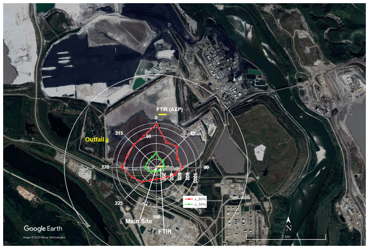
Figure 1 Map of the site: open-path FTIR on the south shore marked in red, open-path FTIR of Alberta Environment and Parks (AEP) on the north shore marked in yellow, and the outfall on the west side. The colored rose plot shows 50 % and 80 % contribution distances for eddy covariance fluxes at 18 m using the Flux Footprint Prediction (FFP) model (Kljun et al., 2015). The unit of contribution distances is in meters. The white circle labels the 2.3 km distance from the main site, equivalent to 100 times the height of the highest point of the top FTIR path. This figure is adapted from You et al. (2020), Fig. 1.

2.2 Open-path Fourier transform infrared spectrometer (OP-FTIR) system

The FTIR measurements were taken with a commercial Open Path FTIR Spectrometer (Open Path Air Monitoring System (OPS), Bruker, Germany), which was set up at 1.7 m above the ground in a trailer. The infrared source is an air-cooled Globar. The emitted radiation is directed through the interferometer where it is modulated, travels along the measurement path (200 m horizontal distance) to a retroreflector array that reflects the radiation, travels back to the spectrometer, and enters a Stirling-cooled mercury cadmium telluride (MCT) detector (monostatic configuration). Three retroreflectors were employed in this study: one near ground level (1 m) on a tripod and two at higher elevations on basket lifts, resulting in heights of reflectors of approximately 1, 11, and 23 m above ground. Three paths with these three retroreflectors are referred to as bottom, middle, and top paths. The bottom retroreflector was approximately twice the size of the upper two (59 vs. 30 reflector cubes). All retroreflectors were cleaned with an alcohol solution once during the study, and the bottom mirror was rinsed with de-ionized water three times. Return signal strength decreased by around 65 % during the 5-week study due to reflector deterioration, presumably mostly due to impaction by particulate matter. This reflector deterioration also decreased the signal-to-noise ratio by around 67 %, based on spectral retrievals for CH₄, but did not affect the mean mole fractions measured.

In this study, spectra were measured at a resolution of 0.5 cm⁻¹ with 250 scans co-added to increase signal-to-noise ratio, resulting in roughly a 1 min temporal resolution. Stray light spectra were recorded regularly by pointing the spectrometer away from the retroreflectors. This stray light spectrum accounts for radiation back to the detector from internal reflections inside the spectrometer, i.e., not from the retroreflector array, and was subtracted from all the measurement spectra before performing further analysis.

Table 1 Spectral windows of OP-FTIR spectra for retrieving mole fractions of pollutants in this study.

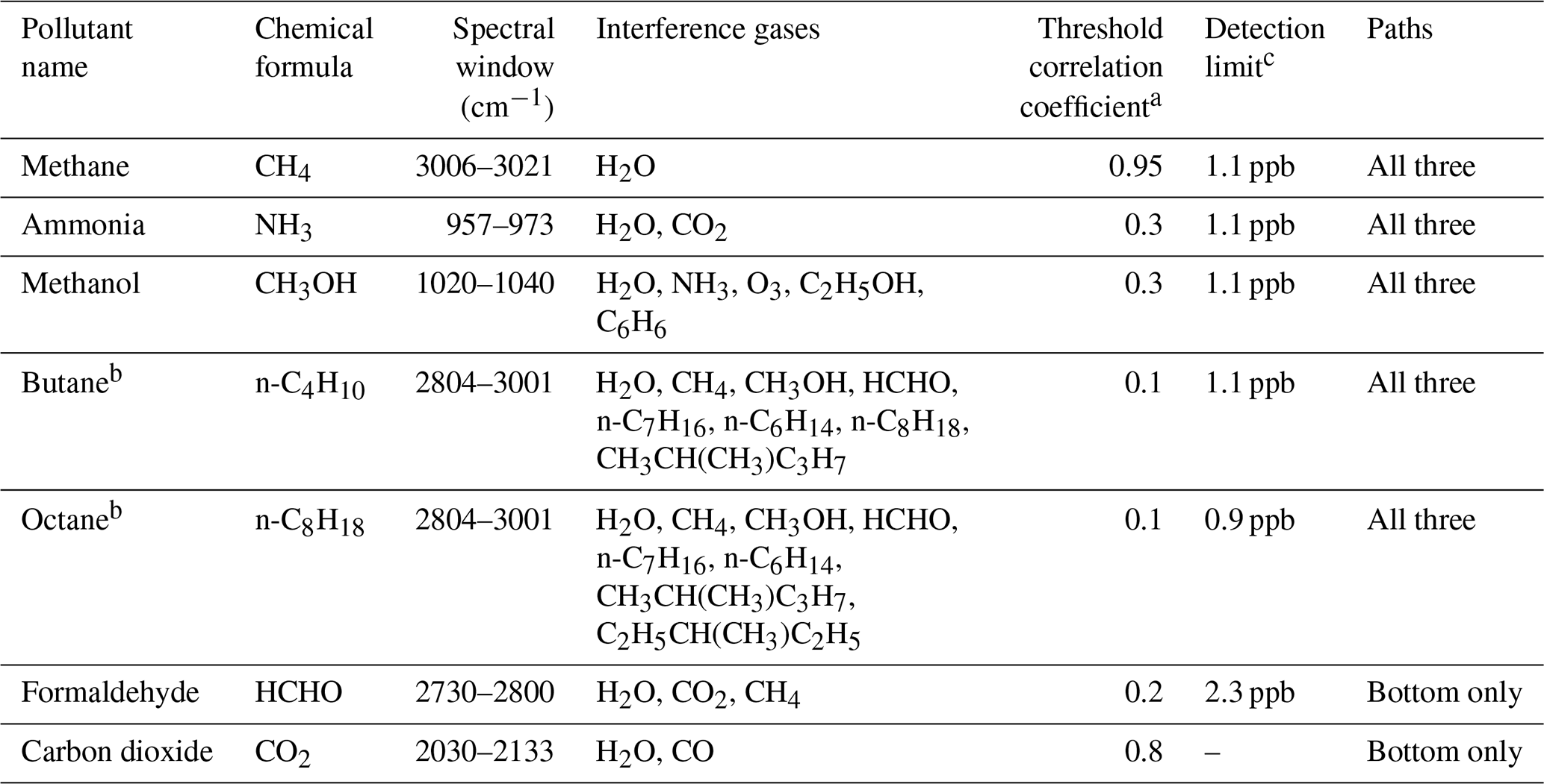
^a Threshold correlation coefficient is a input for OPUS_RS when performing fitting analysis of FTIR spectra. When the correlation coefficient between measured spectrum and reference spectrum with the defined spectral window is below this threshold, that pollutant is not identified and the mole fraction is reported as zero in OPUS_RS (You et al., 2017). ^b Butane and octane mixing ratio are quantified as two surrogates to quantify a total alkane mixing ratio = butane + octane (Thoma et al., 2010). ^c Detection limit is calculated by converting 3σ of the noise of the measurements with a retroreflector distance of 225 m by Bruker to 3σ of the noise with 200 m in this study.

Spectral fitting was performed with OPUS_RS (Bruker), which uses a non-linear curve-fitting algorithm (You et al., 2017). Spectral windows and interference gases for each gas (Table 1) were determined by optimizing capture of the absorption features while minimizing interferences. To further improve fittings, baselines were optimized through either linear or Gaussian fits under given spectral windows and interfering gases. For CH₄ and CO₂, temperature-dependent reference files were used for fitting and retrieving mole fractions. For other pollutants, reference spectra at 296K were used and retrieved mole fractions were corrected for air density using measured ambient temperature and pressure. For the bottom path, the retrieved mole fractions were corrected for the temperature effect given the temperature difference between the temperatures at 8 m (used as the input temperature) and 1 m. For the top path, the retrieved mole fractions were corrected for the temperature effect given the temperature difference between the input temperature at 8 m and the temperature at 12 m (linearly estimated by using temperature at 8 and 18 m). The corrected mole fractions from the three paths were then converted to dry mole fractions using the RH, temperature, and pressure measured at 1, 8, and 18 m. The dry CH₄ mole fractions from FTIR were then calibrated against CH₄ mole fractions from point cavity ring-down spectrometer (CRDS) measurements (Picarro G2204) at 4 m (Sect. S1.1 and Fig. S1 in the Supplement). These calibrated CH₄ mole fractions from the FTIR were then used in flux calculations.

We also attempted to retrieve several other pollutants from measured FTIR spectra but encountered insufficient signal-to-noise ratios, given the existing mole fractions at this location, variability in ambient H₂O vapor, etc. These pollutants include toluene, benzene, xylenes, sulfur dioxide, dimethyl sulfide, carbonyl sulfide, formic acid, and hydrogen cyanide. Given the complex mixture of interfering gas signatures at this site, the detection limits of this open-path system were insufficient for flux calculations.

2.3 Method of deriving gradient flux

2.3.1 Method of deriving eddy diffusivity of gas (K_c)

Gradient flux estimates are derived from the vertical gradient of mole fractions and the associated turbulence, given by

$$\begin{array}{}\text{(1)}& F_c=-K_c{\displaystyle \frac{\partial c}{\partial z}},\end{array}$$

where F_c is the flux for a pollutant gas c, and $\frac{\partial c}{\partial z}$ is the vertical gradient of mole fractions of gas c. K_c is the eddy diffusivity of the gas c, a transfer coefficient characterizing turbulent transport (Monin and Obukhov, 1954) and relating the vertical gradient of gas c to its flux. To calculate the gradient flux of pollutants measured by the OP-FTIR system, K_c has to be calculated first. In this study, K_c is calculated with a variation on the modified Bowen ratio method (Meyers et al., 1996; Bolinius et al., 2016), which was described in detail in You et al. (2020). The key steps are repeated here. With the EC flux of CH₄ measured at 18 m and mole fraction gradient measured at 8 and 32 m by CRDS, K_cwas calculated using Eq. (1). The limitation of using this K_c is that when the vertical gradient $\frac{\partial c}{\partial z}$ is close to zero, both F_c and K_c are poorly defined. A much better behaved eddy diffusivity is that for momentum, calculated by combining the wind profile with the momentum flux (Eq. 2). To construct a continuous time series of K_c for CH₄, we used K_m and the relationship between K_m and K_c in Eq. (3).

$$\begin{array}{}\text{(2)}& {\displaystyle }{F}_{\text{m}}=-K_{\text{m}}{\displaystyle \frac{\partial u}{\partial z}}\text{(3)}& {\displaystyle }{S}_c={\displaystyle \frac{K_{\text{m}}}{K_c}}\end{array}$$

K_c can thus be calculated from K_m if the Schmidt number S_c is known. You et al. (2020) showed the details of two approaches to calculate S_c. In this paper, we took the result of stability-corrected variable S_c from the second approach in You et al. (2020).

2.3.2 Gradient flux based on OP-FTIR measurements

K_c is a function of height above the surface (Monin and Obukhov, 1954). The K_c calculated above applies to a height of 18 m and needs to be adjusted to the OP-FTIR path heights. In this study, the vertical profiles of the CH₄ mole fractions varied over time and mostly showed linear vertical profiles when the wind was from the pond (Sect. S1.2). In the following calculation, the vertical profiles of CH₄ and other gases are considered linear over the entire project. Therefore, the representative average height of the FTIR top path is taken as the height of the middle point (at 12 m). $K_{c_{\mathrm{FTIR}}}$ for gradient flux calculated from the top and bottom FTIR paths has been adjusted linearly based on the $K_{c_{\left(\text{8\hspace{0.17em}m,32\hspace{0.17em}m}\right)}}$ calculated from point measurements at 8 and 32 m on the tower:

$$\begin{array}{}\text{(4)}& {\displaystyle \frac{K_{c_{\mathrm{FTIR}}}}{K_{c_{\text{(8\hspace{0.17em}m,32\hspace{0.17em}m)}}}}}={\displaystyle \frac{\frac{K_{{\text{m}}_{\mathrm{FTIR}}}}{S_c}}{\frac{K_{{\text{m}}_{\text{(8\hspace{0.17em}m,32\hspace{0.17em}m)}}}}{S_c}}}={\displaystyle \frac{K_{{\text{m}}_{\mathrm{FTIR}}}}{K_{{\text{m}}_{\text{(8\hspace{0.17em}m,32\hspace{0.17em}m)}}}}}.\end{array}$$

K_m is a function φ_m, which in turn is a function of stability ($z/L$), where z is the height above ground and L the Obukhov length:

$$\begin{array}{}\text{(5)}& {\displaystyle }{K}_{\text{m}}={\displaystyle \frac{k{u}_{\ast }z}{{\mathit{\phi }}_{\text{m}}}},\text{(6)}& {\displaystyle }{\mathit{\phi }}_{\text{m}}=\left\{\begin{array}{lll}\mathrm{1}+\frac{\mathrm{4.7}z}{L}& \text{for}& \frac{z}{L}>\mathrm{0}\left(\text{stable}\right)\\ \mathrm{1}& \text{for}& \frac{z}{L}=\mathrm{0}\left(\text{neutral}\right)\\ {\left[\mathrm{1}-{\displaystyle \frac{\mathrm{15}z}{L}}\right]}^{-\mathrm{1}/\mathrm{4}}& \text{for}& \frac{z}{L}<\mathrm{0}\left(\text{unstable}\right).\end{array}\right.\end{array}$$

Here u_∗ is the friction velocity. From Eqs. (4)–(6), $K_{{\text{m}}_{\mathrm{FTIR}}}/K_{{\text{m}}_{\text{(8\hspace{0.17em}m,32\hspace{0.17em}m)}}}$ is calculated for each half-hour period. The FTIR gradient flux is then calculated by multiplying this $K_{c_{\mathrm{FTIR}}}$ by the mole fraction gradient between top and bottom path of the FTIR in Eq. (1). The difference between assuming linear and logarithmic vertical profiles of the mole fractions is discussed in the Sect. S1.2. The logarithmic vertical profile assumption resulted in an average flux which is 19 % greater than the average gradient flux calculated with linear vertical profiles.

In addition to calculating gradient fluxes by using the CH₄ mole fraction gradient between top and bottom paths, gradient fluxes of CH₄ were also calculated by using the mole fraction gradient between middle and bottom paths. Results show that the average gradient fluxes with middle-bottom paths gradient are 29 % less than that with top-bottom paths (Sect. S1.2, Table S1). These results suggest the gradient fluxes in this study may include uncertainties from the vertical profile of K_c, which has not been studied much in the past. Lastly, the approach developed by Flesch et al. (2016) was applied and compared to the approach shown above. Fluxes were within 70 %. K_c values for NH₃ and total alkanes are assumed to be the same as K_c for CH₄.

2.3.3 Inverse-dispersion fluxes

Inverse-dispersion models (IDMs) are a useful method for deriving emission rate estimates based on line-integrated or point mole fraction measurements downwind of a defined source. IDMs require inputs including the mole fraction measurements, the surface turbulence statistics between the measurements and the source, and the background mole fraction (mole fraction upwind of the source) of the pollutant. In this study, we used WindTrax 2.0 (Thunder Beach Scientific, http://www.thunderbeachscientific.com, last access: 26 January 2021; Flesch et al., 1995, 2004), which is based on a backward Lagrangian stochastic (bLS) model. Details on IDM calculations and resulting CH₄ fluxes were presented in You et al. (2020). Key information is repeated here. The emission rate is derived through

$$\begin{array}{}\text{(7)}& Q={\displaystyle \frac{\left(C-C_{\mathrm{b}}\right)}{{\left(\frac{C}{Q}\right)}_{\text{sim}}}},\end{array}$$

where C is the mole fraction of the pollutant measured at a given location, C_b is the background mole fraction and $(C/Q{)}_{\text{sim}}$ is the simulated ratio (calculated by the bLS model) of the pollutant mole fraction at the site to the emission rate at the specified source. In this study, the inputs of surface turbulence statistics are u_∗ and L calculated from the ultrasonic anemometer measurements at 8 m, ambient temperature measured at 8 m, and the mean wind direction measured by the propeller anemometer at 4 m. All surface turbulence statistics inputs were half-hour averages. Half-hour periods when u_∗ < 0.15 m s⁻¹ were excluded (Flesch et al., 2004). IDM fluxes of NH₃ and total alkane are shown in this work for the first time for comparison with gradient fluxes. Meteorological inputs for calculating inverse-dispersion fluxes of NH₃ and total alkanes are the same as for CH₄ fluxes. CH₄, NH₃, and total alkanes mole fraction inputs were mole fractions from the bottom path of OP-FTIR.

3 Results and discussion

3.1 Meteorological conditions

The measurement site including the OP-FTIR was at the south shore of the pond (Fig. 1); therefore, the northern wind (wind direction (WD) ≥ 286^∘ or WD ≤ 76^∘ ) was defined as the wind coming from the pond (You et al., 2020). The wind came from the north for about 22 % of the entire measurement period (Fig. S2 in You et al., 2020). There was no significant diurnal variation in wind direction during the study period. Detailed ambient temperature, water surface temperature, wind speed, and other meteorological parameters can be found in You et al. (2020). As discussed in You et al. (2020), the warm pond surface resulted in continuing convective turbulence at night, resulting in continuing transport of pollutants from the pond into the atmosphere without significant diurnal variation.

Gradient and IDM fluxes for NH₃ and total alkanes are averages for half-hour periods when the wind came from the pond. The half-hour fluxes were binned into 16 wind direction sectors, and the area-weighted averages of fluxes from the pond were calculated as described in You et al. (2020).

3.2 Methane

Path-integrated mole fractions and associated gradient fluxes of CH₄ from OP-FTIR are presented here to test if the gradient fluxes derived from the mole fractions with OP-FTIR are comparable to CH₄ fluxes from EC and IDM methods (You et al., 2020). The area-weighted flux statistics from different methods are summarized in Table 2. The path-integrated measurement from the FTIR bottom path clearly indicates that the CH₄ mole fraction was elevated when the wind was from the pond direction, while it was steady near 2 ppm when the wind was from other directions (Figs. S2 and S3). In addition, a clear vertical gradient (Fig. S3), with mole fractions along the bottom path on the order of 0.5 to 1 ppm higher than mole fractions from the top path, identified the pond as the CH₄ source. The fact that the CH₄ mole fraction increased when the wind was from the pond direction, and decreased with height, clearly points to the pond as the dominant local source.

Table 2 Summary of fluxes from OP-FTIR measurements. Results are area-weight-averaged fluxes from the pond.

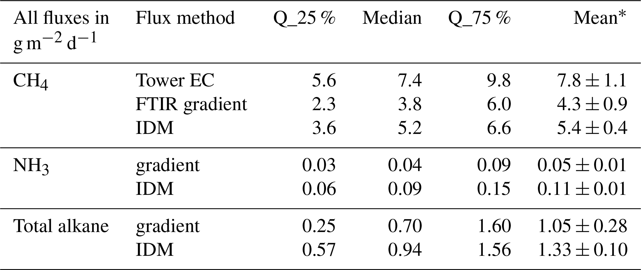
^∗ Errors with the mean fluxes are calculated with a top-down approach: the average of standard deviations of fluxes from five periods when the fluxes displayed high stationarity.

For comparison, vertical profiles of the CH₄ mole fraction by point measurements on the nearby tower are given in Sect. S1.2. A linear vertical extrapolation of the profiles to the point where the mole fraction reaches 2.0 ppm (background levels) indicated a median plume height of 64 m (Figs. S4 and S5).

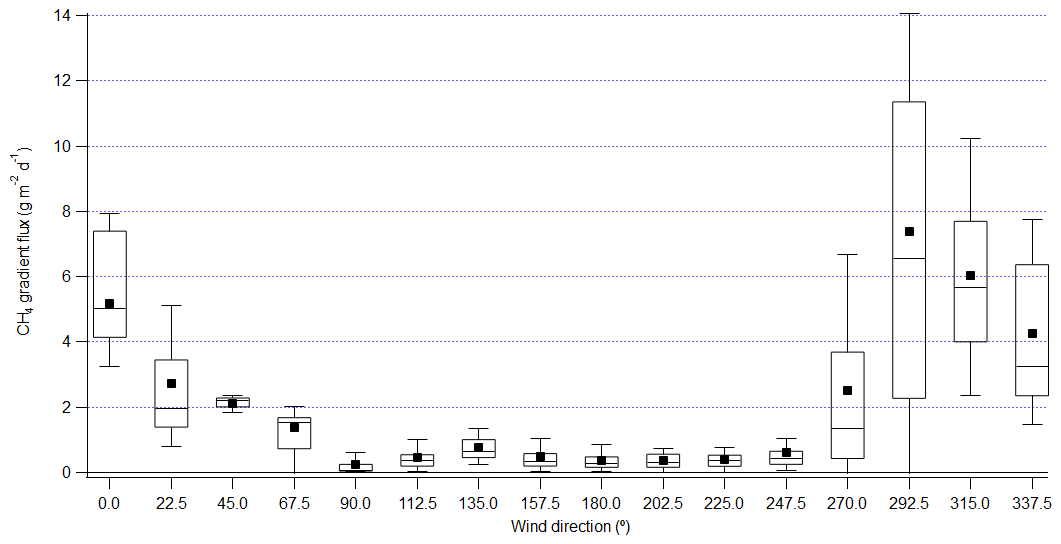
Figure 2 Gradient flux of CH₄ from FTIR binned by wind direction in 22.5^∘ bins. Lower and upper bounds of the box plot are the 25th and 75th percentile; the line in the box marks the median and the black square labels the mean; the whiskers label the 10th and 90th percentile.

The gradient flux derived from the OP-FTIR shows that the flux was minimal when the wind was from other directions, except for the sector centered at 270^∘ (Fig. 2), which represented a mix of pond and shoreline influences. The average and interquartile ranges of fluxes in wind direction sectors centered at 315, 337.5, and 0^∘ are comparable. This gradient flux result is consistent with the EC fluxes measured on the adjacent flux tower (You et al., 2020), and these results also suggest that the pond is the main source of measured CH₄ fluxes. However, the sector centered at 292.5^∘ shows average flux 22 % and 73 % greater than sectors centered at 315 and 337.5^∘. This is different from the EC fluxes, which showed closer agreement between the 292.5, 315, 337.5, and 0^∘ sectors (Fig. 7 in You et al., 2020). The footprint of the EC fluxes measured on the adjacent flux tower at 18 m was calculated by using the Flux Footprint Prediction (FFP) model in Kljun et al. (2015), and results showed the 80 % contribution distance was typically within 1 km, which is closer to the main site than the north edge of pond liquid surface (Fig. 1; You et al., 2020). The outfall was about 1.4 km from the main site. The discrepancy suggests that the footprint of the gradient method incorporated emissions from the outfall more clearly than the smaller footprint of the EC method.

FTIR CH₄ gradient fluxes and EC fluxes showed a linear correlation, but on average the gradient fluxes were lower than the EC fluxes by 44 % (r² = 0.63) (Fig. S7). In agreement with EC, the gradient flux showed no significant diurnal variations when the wind was from the pond (Fig. S8, with a relative standard deviation of 38 %). To investigate the difference between CH₄ gradient fluxes derived from FTIR and EC fluxes, the latter were examined in relation to meteorological conditions, similar to the analysis presented in You et al. (2020). The analysis in You et al. (2020) showed weak correlation between EC flux and friction velocity (u_∗) or wind speed, consistent with the observation of the weak correlation between gradient flux and wind speed (Fig. S5 in You et al., 2020). As described in Sect. S1.2 (Figs. S4, S5, and S6), CH₄ vertical profiles were closer to linear when the wind speed was less than 6 m s⁻¹ and were more logarithmic with wind speed greater than 6 m s⁻¹. The sector centered at 292.5^∘ was often associated with wind speeds greater than 6 m s⁻¹ (21 % of the time). The approximation of linear vertical profile could have underestimated the CH₄ flux with periods of high winds by 19 %. This weak dependence of gradient flux on wind speed may reflect the uncertainty in the vertical profile of K_c in the calculation of gradient flux.

Model calculations by Horst (1999) showed that the estimated footprint of a gradient flux measurement at the geometric mean height of the gradient is similar to the footprint of EC flux at that same height for homogeneous upwind area sources. However, mole fraction footprints are significantly larger than perturbation (flux) footprints (Schmid, 1994), and some CH₄ sources on the far shore (e.g., the outfall) may have contributed to the upper-path CH₄ mole fraction. This decreased the vertical gradient difference and thus the derived flux relative to the EC flux with its smaller footprint, since the latter is more likely to represent water surface emissions only. As an approximate estimation, the footprint of the path-integrated mole fraction of the top path is about 2.3 km (23 m × 100; Flesch et al., 2016), and this covers the whole pond including the north edge (Fig. 1).

Background mole fractions, upwind of the source under investigation, must be provided for the bLS calculations of CH₄ fluxes. We quantified these using two methods. First, the background mole fraction was determined with the FTIR measurements at the south of the pond, as follows: for most of the days, it was taken as the minimum CH₄ mole fraction from the FTIR bottom path on each day while the wind direction was between 180 and 240^∘. On 7 and 30 August, there was no half-hour period when the wind was from this sector, and the background mole fraction was chosen as the minimum mole fraction for the day. For 1 August, there was also no half-hour period for this sector, and the minimum of the day was 2.40 ppm, significantly greater than the minimum mole fraction of other days. Therefore, the background mole fraction of the previous day, 1.92 ppm, was used for 1 August.

Alberta Environment and Parks (AEP) conducted OP-FTIR measurements (RAM2000 G2; KASSAY FSI, ITT Corp., Mohrsville, PA, USA) at the north side of the pond (Fig. 1), quantifying CH₄ to be used as the second estimate of background mole fractions. For most of the days, the half-hour averaged mole fractions were directly used as the background mole fractions. From 3 August 22:00 to 4 August 13:30, 6 August 08:00 to 17:00, and 23 August 01:30 to 02:00 UTC there were no data from AEP, so background mole fractions for these periods were picked as the interpolation of mole fractions before and after this period. In this approach, the bLS flux results can be negative when the AEP mole fraction is greater than the mole fraction from the measurements at the south shore, possibly due to influences by other emission sources in the surrounding area, gas diffusion under low wind speeds, plume inertia when wind direction changes suddenly, or instrument mismatch differences.

CH₄ IDM fluxes with background determined from the first approach (using measurements at the south of the pond) agreed with IDM fluxes with background determined from the second approach (using measurements at the north of the pond), with a linear regression r² of 0.92 and a slope of 0.90; there was a 20 % difference between average fluxes from the two approaches (Fig. S10; Table S1). These results confirm that the CH₄ flux estimate from this inverse-dispersion approach is consistent and that the first approach to determining backgrounds is appropriate. In the following results and discussion, IDM fluxes with background mole fractions from the first method are used.

IDM and EC flux showed moderate comparison (slope = 0.69, r = 0.62; Fig. S7 in You et al., 2020), although the mean IDM fluxes are 30 % smaller than the EC flux.

3.3 NH₃

The mole fraction of NH₃ was elevated when the wind was from the pond but was mainly below 5 ppb when the wind was from the south (Fig. 3a). NH₃ gradient fluxes were significant when the wind came from the pond direction (Fig. 4a).

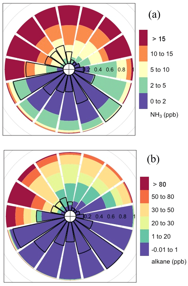
Figure 3 Normalized rose plot of NH₃ (a) and total alkane (b) mole fractions from FTIR bottom path. Colors represent the mole fraction in part per billion. The length of each colored segment presents the time fractions of that mole fraction range in each direction bin. The radius of the black open sectors indicates the frequency of wind in each direction bin; the angle represents wind direction – straight up is north and straight left is west.

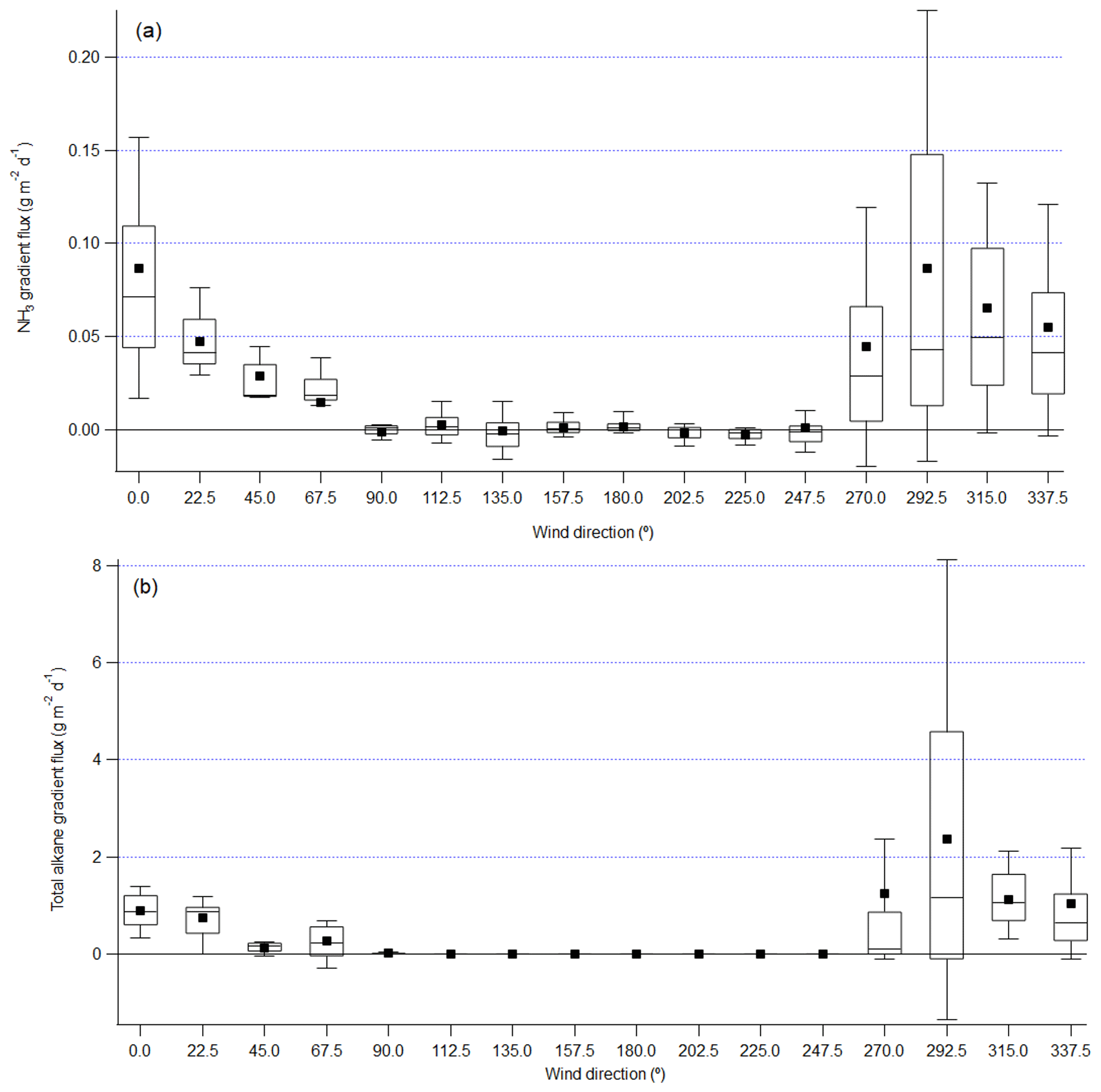
Figure 4 Gradient flux of NH₃ (a) and total alkane (b) from FTIR top-bottom path binned by wind direction in 22.5^∘ bins. Lower and upper bounds of the box plot are the 25th and 75th percentile; the line in the box marks the median and the black square labels the mean; the whiskers label the 10th and 90th percentile.

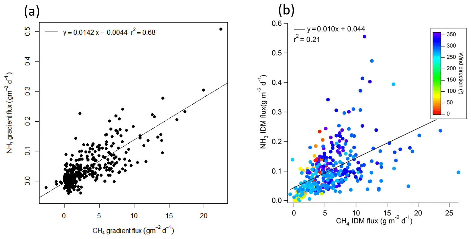
Figure 5 (a) NH₃ gradient flux compared to CH₄ gradient flux; (b) NH₃ IDM flux compared to CH₄ IDM flux.

The time series of mole fraction vertical gradient of NH₃ and CH₄ were similar (Figs. S3 and S12). The NH₃ gradient flux and CH₄ gradient flux showed good correlation (r² = 0.7, Fig. 5a). The diurnal variation in the NH₃ gradient flux (relative standard deviation = 72 %) was stronger than for the CH₄ gradient flux (relative standard deviation = 36 %), with greater fluxes from 13:00 to 18:00 MDT (mountain daylight savings time) (Fig. S11a). Previous studies showed tailings pond waters contained elevated NH₃ concentrations, which makes them potential sources of NH₃ to the atmosphere (Allen, 2008; Risacher et al., 2018). NH₃ in the pond is mainly produced through nitrate and/or nitrite reduction during microbial activities (Barton and Fauque, 2009; Collins et al., 2016). In addition, some of these nitrate and/or nitrite reduction microbes may also produce reduced sulfur (Barton and Fauque, 2009). The water sample collected from Pond 2/3 on August 2017 during this study was alkaline (pH = 8.0 ± 0.5), which also supports the emission of NH₃.

The average flux in the sector centered at 292.5^∘ was 33 % and 57 % more than the average flux in the sectors centered at 315 and 337.5^∘, but the median fluxes in these three sectors are within 14 %. These suggest the high average flux in 281–304^∘ is skewed by big spikes which are associated with the outfall (with wind directions in 281–304^∘), but the majority of NH₃ fluxes in the 281–304^∘ wind sector correlated well with CH₄ fluxes which were less affected by the outfall. Although hydrotreating processes in upgraders remove most of the sulfur and nitrogen from the bitumen residue, a small amount of NH₃ might still be carried with the processed water and tailings (Bytnerowicz et al., 2010) and transported with the outfall liquid into the pond. The negative fluxes observed for the 67.5^∘ sector may be due to elevated NH₃ plumes originating from the upgrader facility 3 km upwind in this direction, resulting in a negative gradient and thus deposition to the pond under some circumstances.

IDM fluxes of NH₃ were calculated the same way as CH₄ and show a weak correlation with CH₄ IDM fluxes (Fig. 5b). The NH₃ background mole fraction was based on the mean daily minimum, approximately 1 ppb (Fig. 3). Vertical profiles of NH₃ mole fraction (Fig. S12) with northerly wind also show roughly linear profiles similar to CH₄. Profiles of sectors centered at 292.5 and 315^∘ are linear. Therefore, the outfall on average did not significantly contribute to the NH₃ profile; i.e., the pond surface was the main source of NH₃. NH₃ fluxes from the gradient method were significantly less than from the IDM method. This difference is mostly due to the input background NH₃ mole fraction. The background NH₃ mole fraction was not measured and could be greater than 1 ppb if there was any source to the north of the pond. Assuming the NH₃ gradient flux as a reference, different backgrounds were tested in IDM to match the mean gradient flux. A background of 7 ppb of NH₃ was required to close the gap between gradient and IDM fluxes. This seems large but cannot be verified, since there was no ground level measurement of NH₃ near the north of the pond. This illustrates the advantage of using either EC or gradient flux measurements, which are based on mole fraction fluctuations or gradients at a single location and are therefore independent of upwind background mole fraction.

3.4 Total alkane

Total alkane derived from FTIR spectra used butane and octane as two surrogates in this study, following the method in EPA OTM 10 (Thoma et al., 2010). Results only reflect alkanes which have similar absorption features to butane and octane and cannot accurately represent other VOCs. Total alkane fluxes from the pond were evident (Fig. 4b). A comparison to CH₄ fluxes showed only a weak correlation (r² = 0.3, Fig. S13), unlike the correlation between NH₃ and CH₄ (Fig. 5a). This difference can be explained by sources of alkane and CH₄ at this site. Figure 4b shows the average flux from the sector centered at 292.5^∘ is 2.4 g m⁻² d⁻¹, which is 2.09 and 2.29 times of the average fluxes from the sectors centered at 315^∘ and 337.5^∘. Figure 2 shows that the average fluxes of CH₄ from the sector centered at 292.5^∘ is 1.22 and 1.72 times of the average fluxes from sectors centered at 315 and 337.5^∘. These results indicate that there was an enhanced contribution (27 %) from around 281 to 304^∘ to total alkane flux measured at the site but not to the observed CH₄ flux. This enhancement of alkane flux is likely due to the outfall, which was at the edge of the pond, 1.9 km from the site at 295^∘. The liquid mixture flowing into the pond contained naphthenic solvent, which includes a mixture of alkanes, alkenes, and aromatic hydrocarbons, and since the outfall is at a temperature of approximately 33 ^∘C, enhanced evaporation of volatile components can be expected from this area. The outfall also introduces some mechanical mixing in the upper layers of the pond water, which may contribute to elevated emission rates. The diurnal variation of total alkane gradient flux when the wind came from the pond direction was also weak (the standard deviation of average fluxes at each hour is comparable to the interquartile ranges, Fig. S14). The vertical profiles of total alkane mole fraction with northeastern winds were vertically invariant (Fig. S15). With northwestern winds, profiles showed a decreased mole fraction from the bottom to middle path and a minimal decrease or even increase from the middle to the top path. These total alkane vertical profiles with northern wind are different from CH₄ or NH₃ profiles with the same periods, suggesting there were additional sources other than the pond surface to the measured total alkane flux, such as the outfall and industrial activities upwind. IDM flux of total alkanes agreed moderately with gradient flux, with a difference of 21 % (26 %) in the pond average (median) flux.

3.5 Methanol (CH₃OH)

Unlike pollutants studied above, the CH₃OH mole fraction did not show significant enhancement when wind was from the pond (Fig. S16), suggesting the pond was not significantly contributing to CH₃OH compared to potential sources surrounding the pond. The calculation of the gradient flux of CH₃OH was attempted in the same way as for the other pollutants, and the flux was on the order of 1 mg m⁻² d⁻¹ but with an uncertainty that made it not statistically different from zero. The lifetime of CH₃OH is around 10 d (Simpson et al., 2011; Shephard et al., 2015), and the main source is vegetation (Millet et al., 2008). The mole fractions observed at the site were consistent with satellite measurements representative of the general oil sands region (Shephard et al., 2015) and with an airborne study of VOCs (Simpson et al., 2010). In addition to emissions from vegetation, CH₃OH observed in the oil sands region could be due to transport from biomass burning (Simpson et al., 2011; Bari and Kindzierski, 2018) and local traffic (Rogers et al., 2006; You et al., 2017).

3.6 Comparison of calculated fluxes to reported emissions and approaches

As a test of the robustness of these results, fluxes of CH₄, NH₃, and total alkane are also calculated from the slant path method described by Flesch et al. (2016). Calculation inputs and results are summarized in the Sect. S5. Compared to results from our flux-gradient approach, CH₄, NH₃, and total alkane fluxes with the slant path flux-gradient method were reasonably comparable (24 %, 25 %, and 30 % lower, respectively; Table S1). The difference in fluxes from the two approaches could be due to differences in assumptions regarding the vertical profiles. In our gradient flux approach, we used linear vertical mole fraction profiles of pollutants to calculate the difference of mean heights between the two paths. In Flesch et al. (2016) the gradient flux for pairs of points along the two paths was integrated along the entire path length assuming the flux was uniform horizontally. In that approach, the dependence of K_c on height is incorporated explicitly, assuming a logarithmic wind profile including a stability correction. In our gradient flux approach, K_c is derived from a measured and stability-corrected K_m and therefore did not require a wind profile shape assumption.

To facilitate a transparent comparison of the emission results from this study to reported facility-wide emissions of Suncor, we present emission rates based on simple extrapolation of the measured August emissions to the whole year. Other possible seasonal emission profiles have been reported (Small et al., 2015); using these to convert from August emissions to annual average values would for example result in a scale factor of 0.92 (mass transfer model), 0.64 (mass transfer model adjusted for ice cover), or 0.42 (thawing degree-day model) (Cumulative Environmental Management Association, 2011). The seasonally invariant total emission estimates for NH₃ and total alkanes from Pond 2/3 to the air were 42 and 881 t yr⁻¹ in 2017, converted from gradient fluxes results in g m⁻² d⁻¹. However, NH₃ emissions from Pond 2/3 have not been reported in the past, because NH₃ was not being measured as part of compliance flux chamber monitoring. Therefore, the facility-wide NH₃ emissions reported to the Government of Canada National Pollutant Release Inventory (NPRI) (0.82 t yr⁻¹) in 2017 did not include fugitive emissions from tailings ponds. The solvents entering this tailings pond are naphtha additives with octane, nonane, and heptane as the biggest contributors. Li et al. (2017) quantified alkane emissions (including n-alkanes, branched alkanes, and cycloalkanes) as 36.2 t d⁻¹ from the whole facility using airborne measurements in 2013, which is 73.9 % of 49 t d⁻¹ total VOC emission. Alkanes account for 54 % of total VOC emitted from Pond 2/3 in 2017 (internal communication with Samar Moussa). If we use reported facility-wide VOC annual emissions in 2017 (17 242 t yr⁻¹, NPRI) to estimate facility-wide total alkane annual emission, we obtain 17 242 × 53 % = 9138 t yr⁻¹, and total alkane emissions from Pond 2/3 contribute 9.6 % to facility-wide emissions for 2017. The fugitive NH₃ emissions from Pond 2/3 in this study were 42 t yr⁻¹, a number that is 51 times the process-related emission number reported for the facility to NPRI. Negligible volume of ammonia may be carried over to the pond through the naphtha recovery unit and froth treatment tailings (FTT) line, and it is believed that the ammonia is mainly generated from the biogenic activities in the mature fine tailings (MFT) layer of the pond. The majority of H₂S, NH₃, and CH₄ emissions are related to microbiological activities as evidenced in this study.

4 Conclusions and implications

We have shown that OP-FTIR is an effective method to quantify mole fractions and vertical gradients of CH₄, NH₃, and total alkanes continuously and simultaneously for an area source such as a tailings pond. Benefits are the integration of mole fractions over long path lengths, thus providing a spatially representative average, and the avoidance of sample line issues that can be serious problems for sticky gases such as NH₃. Results from the gradient flux method and IDM calculations suggest OP-FTIR is a useful tool for deriving emission rates of CH₄, NH₃, and total alkane from this type of fugitive area source. For the two approaches for determining background mole fractions of CH₄ with the IDM method, i.e., upwind background measurement vs. local background estimation, the area-weight-averaged fluxes of CH₄ were within 20 %. FTIR CH₄ gradient fluxes and EC fluxes showed a linear correlation, but on average the gradient fluxes were lower than the EC fluxes by 44 %. CH₄ IDM and EC flux showed moderate comparison, and the mean IDM fluxes are 30 % smaller than the EC mean flux. NH₃ gradient flux and IDM flux showed a difference of more than 50 %, which suggests that there may have been sources of NH₃ upwind (north) of the pond that were not captured by assuming that southern and northern background NH₃ were similar, thus illustrating a limitation of the IDM method. CH₄, NH₃, and total alkane fluxes were also calculated using the slant path flux-gradient method (Flesch et al., 2016), to compare to the our flux-gradient approach, and results from the slant path method were reasonably comparable (24 %, 25 %, and 30 % lower, respectively).

The NH₃ emissions results in this study are the first to quantify NH₃ fugitive fluxes from a tailings pond and clearly showed that Pond 2/3 is a significant source of NH₃, most likely through microbial activities in the pond. This suggests that at least some tailings ponds in the oil sands could be significant sources of NH₃, compared to process-related facility emissions. Further measurements of NH₃ emissions from tailings ponds are recommended to elucidate our understanding of the mechanisms behind NH₃ emissions and to improve the total facility emission estimates reported to NPRI.

Total alkane gradient fluxes from OP-FTIR measurements clearly showed that the pond is a significant source of total alkane, and annual alkane emissions extrapolated from gradient flux method represented 9.6 % of facility emissions. The outfall area contributed significantly (27 %) to pond alkane emissions, showing spatial variability of alkane emissions from the pond. Observed CH₃OH mole fractions show that the pond was not likely a significant source of CH₃OH. This study demonstrated the applicability of OP-FTIR combined with gradient flux or inverse-dispersion methods for determining emission fluxes of multiple gases simultaneously, with high temporal resolution and comprehensive spatial coverage.