the Creative Commons Attribution 4.0 License.
the Creative Commons Attribution 4.0 License.
 | 05 Jan 2022
New sampling strategy mitigates a solar-geometry-induced bias in sub-kilometre vapour scaling statistics derived from imaging spectroscopy
David R. Thompson
Marcin J. Kurowski
Matthew D. Lebsock
Upcoming spaceborne imaging spectrometers will retrieve clear-sky total column water vapour (TCWV) over land at a horizontal resolution of 30–80 m. Here we show how to obtain, from these retrievals, exponents describing the power-law scaling of sub-kilometre horizontal variability in clear-sky bulk planetary boundary layer (PBL) water vapour (q) accounting for realistic non-vertical sunlight paths. We trace direct solar beam paths through large eddy simulations (LES) of shallow convective PBLs and show that retrieved 2-D water vapour fields are “smeared” in the direction of the solar azimuth. This changes the horizontal spatial scaling of the field primarily in that direction, and we address this by calculating exponents perpendicular to the solar azimuth, that is to say flying “across” the sunlight path rather than “towards” or “away” from the Sun. Across 23 LES snapshots, at solar zenith angle SZA = 60∘ the mean bias in calculated exponent is 38 ± 12 % (95 % range) along the solar azimuth, while following our strategy it is 3 ± 9 % and no longer significant. Both bias and root-mean-square error decrease with lower SZA. We include retrieval errors from several sources, including (1) the Earth Surface Mineral Dust Source Investigation (EMIT) instrument noise model, (2) requisite assumptions about the atmospheric thermodynamic profile, and (3) spatially nonuniform aerosol distributions. By only considering the direct beam, we neglect 3-D radiative effects such as light scattered into the field of view by nearby clouds. However, our proposed technique is necessary to counteract the direct-path effect of solar geometries and obtain unique information about sub-kilometre PBL q scaling from upcoming spaceborne spectrometer missions.
- Article
(2600 KB) - Full-text XML
-
Supplement
(1115 KB) - BibTeX
- EndNote


© 2022 California Institute of Technology. Government sponsorship acknowledged.
Spatial scaling in the variability of atmospheric properties such as water vapour (q) can be characterised via structure functions, with the nth-order structure function of a field f(x), Sn defined as
where E[] is the expected value, x a location, and r a separation between points. Fields of temperature (T), q, and wind speed are commonly well modelled by a power law:
such that ζn is the log–log gradient of Sn as a function of r. There is strong motivation to quantify and understand these exponents and the ranges Δr within which they are valid, and here we specify second-order structure functions S2 with exponent ζ2, describing variance scaling. This is related to the commonly referenced Fourier power spectrum exponent β:
One motivation for obtaining these exponents is that climate model sub-grid variability in q is strongly linked to cloud formation (Golaz et al., 2002; Perraud et al., 2011; Sommeria and Deardorff, 1977). In principle, sub-grid variance can be tuned for each model set-up, but scale-aware variance relationships allow a smooth and consistent transition between low-resolution (order ∼ hundreds of kilometres) and high-resolution (order ∼ km) models (Arakawa et al., 2011; Schemann et al., 2013).
At scales larger than model grid cells, observational estimates of variance scaling can also be used to assess model performance, as has been done using estimates of temperature (T) and q from Atmospheric Infrared Sounder (AIRS) and airborne campaign data (Kahn et al., 2011).
Furthermore, the scaling exponents are related to the physical processes that generate the cascade of turbulent eddies in the atmosphere. For example, while mean-scale statistics retrieved by AIRS are approximately isotropic in the horizontal, there are differences in scaling between the horizontal and vertical (Pressel and Collins, 2012). Scaling following is predicted for a passive tracer in the inertial range of 3-D locally isotropic turbulence following Kolmogorov theory. Accounting for the buoyancy effects can strongly modify that scaling (Bolgiano, 1959; Obukhov, 1959), with different exponents expected for the velocity (–) and scalars (), as shown in e.g. Kunnen et al. (2008), Wroblewski et al. (2010), or Boffetta et al. (2012). Exponents of have been commonly measured for vertical wind profiles from dropsondes (Lovejoy et al., 2007), and values typically near ζ2 of for horizontal water vapour in non-convective areas and ζ2=0.72 in convective areas have been determined from airborne lidar retrievals over horizontal ranges of up to 100 km (Fischer et al., 2012, 2013); meanwhile, the sub-kilometre regime remains undermeasured.
Of particular interest for modellers is the existence of “scale breaks”, distances at which the exponents change such that a smooth transition between model resolutions may not be possible. These have been calculated to occur at distances over a broad range of 10–1000 km (Bacmeister et al., 1996; Gage and Nastrom, 1985; Kahn et al., 2011; Pinel et al., 2012), and the range of scales has been speculated to be related to the size of convective systems (Dorrestijn et al., 2018) or changes in the nature of turbulence (Kurowski et al., 2015; Skamarock et al., 2014).
This study focusses on the estimation of horizontal scaling of clear-sky TCWV at sub-kilometre scales and specifically on the integrated PBL water vapour which we refer to as the partial column water vapour (PCWVPBL). Recent work using airborne data (Thompson et al., 2021) and large eddy simulation (LES) output (Richardson et al., 2021a) has provided evidence that sub-kilometre horizontal variability in total column water vapour (TCWV) is almost perfectly correlated with PCWVPBL variability, such that high-spatial-resolution retrievals of TCWV from visible and shortwave infrared (VSWIR) imaging spectrometers can provide unique information about PBL q variability. This is not a statement that all water vapour is inside the PBL but rather that on sub-kilometre spatial scales, the variability in low-altitude water vapour dominates the horizontal column variability. It remains a challenge to disentangle variability from different heights within the PBL such as the sub-cloud layer or a conditionally unstable cloud layer, which may have different scaling properties.
In particular, the PBL depth is typically 1–2.5 km in these simulations, while we obtain variability statistics over horizontal ranges of under 1 km. The vertical averaging over a scale larger than the horizontal calculation means that the interpretation of the physical meaning of the derived exponents is challenging and may not be directly related to the theoretically derived exponents discussed above. This study aims only to determine whether the measurement problem of the solar path can be overcome and leaves the physical interpretation beyond its scope. This point will be revisited in Sect. 4.
Several modern and upcoming missions obtain or will obtain VSWIR spectra that could allow retrieval of TCWV at horizontal resolutions from 20 to 100 m. Current examples include the Multi-Spectral Imager (MSI) on Sentinel-2 (Drusch et al., 2012), the PRecursore IperSpettrale della Missione Applicativa (PRISMA, Candela et al., 2016), and the DLR Earth Sensing Imaging Spectrometer (DESIS, Krutz et al., 2019). Upcoming missions such as NASA's Earth Surface Mineral Dust Source Investigation (EMIT; Green and Thompson, 2020) and ESA's Copernicus Hyperspectral Imaging Mission for the Environment (CHIME; e.g. Rast et al., 2019) will obtain a horizontal resolution of order 30–80 m, and this study will assess performance assuming footprint sizes of 40–50 m, i.e. at the mid-point of that range.
This footprint selection was made based on the resolution of available LES output, and the analysis method is based on the output of retrievals developed specifically for EMIT, which primarily retrieves TCWV to allow atmospheric correction for its surface reflectance target observable. Other instruments such as PRISMA or MSI may have different error characteristics, but we treat retrieval errors in a general manner that could be expanded to these other instruments.
This study attempts to determine whether EMIT will be able to obtain ζ2 over 0.5–1 km after accounting for (1) random retrieval error, (2) systematic biases in retrieval mean and sensitivity, and (3) solar zenith angle.
The PBL is of particular interest since it is the location where reflective low clouds form, and in the Dorrestijn et al. (2018) analysis, ζ2 varied more in the 850 hPa layer than the 300 or 500 hPa layers. However, previous analyses have generally been restricted to far larger spatial ranges, with Dorrestijn et al. (2018) referring to 55–165 km scale variance as occurring at the “tiny scale”. Other examples at higher resolution generally use airborne measurements, with few calculations for separations under 1 km using onboard sensors (Cho et al., 1999), using lidar at 5–100 km (Fischer et al., 2013), or evaluating simulations with lidar for separations > 11 km (Selz et al., 2017).
This study uses LES outputs and does not make any statements about the realism or cause of the LES output ζ2 values but instead aims solely to identify and quantify retrieval biases and errors. Its greatest contribution is to demonstrate that directional calculation strategies can remove biases in estimates of ζ2 introduced by the direct-beam component of the solar path through the atmosphere.
We show that, in a set of 23 LES snapshots, the non-vertical direct-beam path prevents accurate retrieval of sub-kilometre ζ2 when standard methods are naïvely applied. However, errors in ζ2 depend on the direction in which it is calculated relative to the solar azimuth, and selecting the correct solar-aware direction eliminates the bias and therefore overcomes a fundamental barrier to VSWIR estimation of sub-kilometre q scaling. Diffuse sunlight is handled through a plane-parallel radiative transfer approximation, which means that complex 3-D radiative effects are neglected. In clear-sky areas near clouds, 3-D effects can brighten observed spectra (Várnai and Marshak, 2009), with induced biases of order ∼ 0.25 % for VSWIR column CO2 retrievals (Massie et al., 2021). The consequences for hyperspectral TCWV retrievals at 30–80 m horizontal resolution are not currently known, although the effect on retrieved ζ2 would depend on the spatial scaling of these TCWV biases. In Sect. 4 we propose a field experiment design to test our conclusions. Spaceborne spectrometers measure light that has passed along some path, , consisting of downward (Sun-to-surface, r↓) and upward (surface-to-sensor, r↑) components. Retrievals will respond to the path-integrated water vapour (PIWV) between the surface and top of atmosphere (TOA):
Meanwhile the commonly desired value is the vertically integrated water vapour, TCWV:
For a horizontally uniform q field (equivalent to “plane-parallel” in radiative transfer parlance) there is a simple geometric relationship between the two:
where μ is the cosine of the sensor-viewing zenith angle and μ0 the cosine of the solar zenith angle. Despite the fact that real q fields vary horizontally such that Eq. (6) is not strictly true, the VSWIR community commonly assumes a plane-parallel atmosphere and reports the retrieved value as being TCWV (Carbajal Henken et al., 2015; Diedrich et al., 2015; Grossi et al., 2015; Nelson et al., 2016; Noël et al., 2004; Preusker et al., 2021). Here we calculate PIWV by tracing solar rays through 3-D LES output, but for consistency with VSWIR literature terminology, we relate it to an effective TCWVeff:
Our retrieved values, TCWVret, refer to estimates of this property. Figure 1 compares the true TCWV with TCWVeff derived from ray tracing through 3-D LES output when solar zenith angle SZA is 45∘ and solar azimuth is at 0∘, meaning that the horizontal component of r↓ is in the negative y direction. There is an apparent “smearing” from Fig. 1a to b in the y direction, so we refer to these solar-geometry-induced changes in TCWVeff due to the horizontal variability in the q field as the “solar smearing” effect (for a simplified illustration of the physical principles behind why our strategy is anticipated to reduce biases in ζ2, see Figs. S1–S3 in the Supplement).
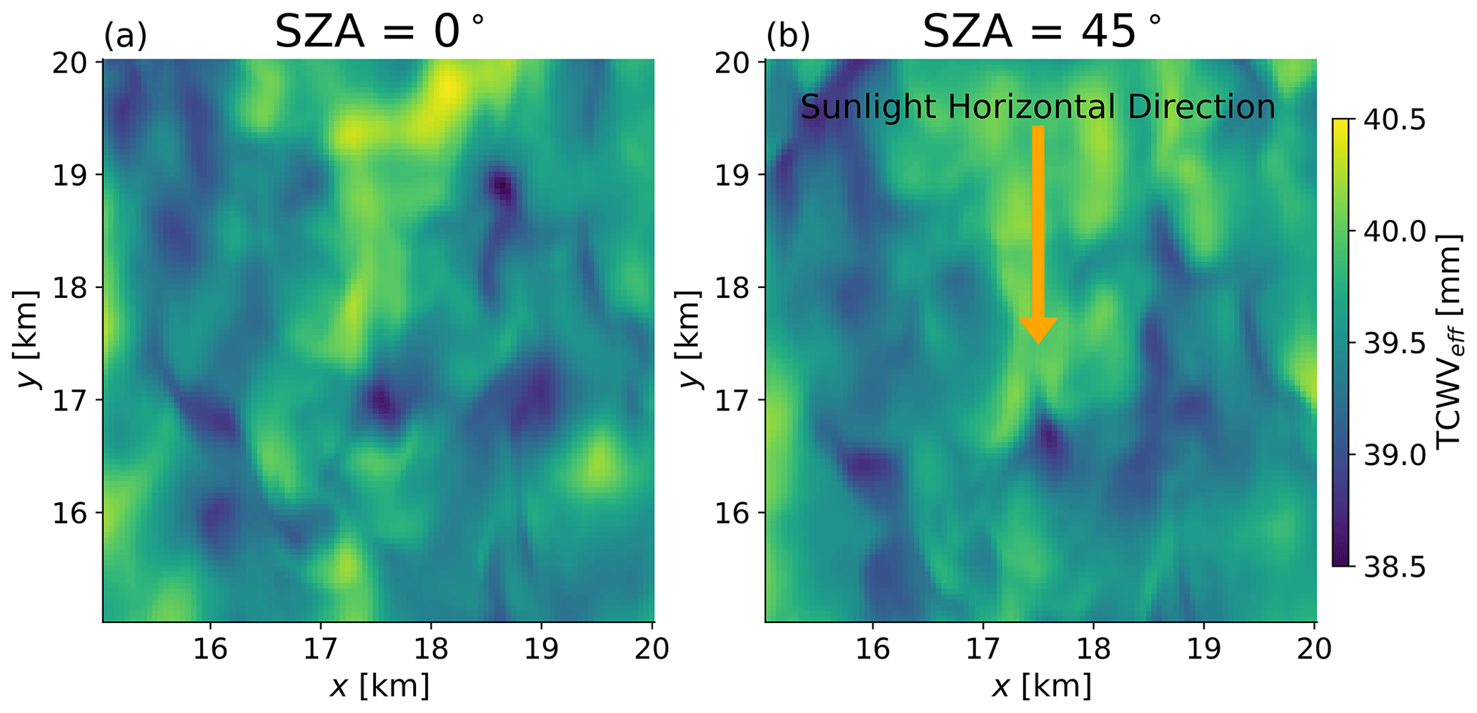
Figure 1Integrated water path in a subsection of the ARM_18000s snapshot (a) in vertical columns directly over each footprint (i.e. true TCWV) and (b) encountered by sunlight with SZA = 45∘ viewed from nadir. The yellow arrow indicates the horizontal direction of the downward solar path.
This consequence of solar and view geometry is well known; for example, Thompson et al. (2021) only used flight lines with very low SZA to minimise its effect in a study of ζ2. However, this severely limits viable data, so here we suggest a new method that exploits the directionality of the solar-smearing effect in order to perform such calculations across a wider range of conditions. This paper uses the solar-path-traced outputs of Richardson et al. (2021a) to demonstrate that by calculating the structure function in a direction perpendicular to the solar azimuth, the bias in ζ2 is removed within the 23 LES snapshots considered. To our knowledge, this is the first quantification of such a technique to mitigate solar-geometry-induced errors in spatial statistics of retrieved atmospheric properties.
If this result can be extended to the real world, then upcoming high-spatial-resolution spaceborne VSWIR spectrometers will provide a breakthrough for analysis of moisture scaling across unprecedented spatial scales. Our retrievals are restricted to clear-sky areas over land, but this still represents a substantial advance in the current capacities of other instrument types. Lidar measurements avoid the solar-path issue and can retrieve vertical information including above clouds, but current and anticipated spaceborne lidars do not offer VSWIR's fine spatial resolution or broad spatial coverage from a wide swath. Sounders such as infrared can profile the atmosphere but have footprints that are too large for sub-kilometre exploration.
Even airborne measurements, which offer far less coverage than spaceborne sensors, may suffer from their own challenges. Evidence suggests that the tendency of flights to follow isobars rather than maintain altitude can introduce height variations that blend vertical variation into horizontal calculations and result in exponents similar to those predicted due to buoyancy's vertical effect (Lovejoy et al., 2004; Pinel et al., 2012).
The VSWIR sampling technique introduced here could greatly expand the range of conditions under which spatial scaling of water vapour can be quantified. In Sect. 2 we describe the LES output, simulated retrievals, and how retrieval errors and solar path are accounted for in calculation of ζ2. Section 3 presents the results and Sect. 4 discusses and concludes.
2.1 Large eddy simulation output
We use q and cloud water (qc) output from the five LES runs of shallow convection as in Richardson et al. (2021a), with four cloudy cases (ARM, ARM_lsconv, BOMEX, RICO) and one case in which clouds do not form (DRY). Simulations use two models, EULAG for the ARM cases (Prusa et al., 2008) and JPL-UCONN LES for the others (Matheou and Chung, 2014). Simulation set-ups are described in Richardson et al. (2021a) and the associated references (Brown et al., 2002; Kurowski et al., 2020; Matheou and Chung, 2014; Siebesma et al., 2003; vanZanten et al., 2011), and while some simulations represent oceanic boundary layers, we simply assume a land surface for the retrievals. Static reanalysis profiles from MERRA-2 (Gelaro et al., 2017) are appended above the LES domain, but the LES domains were shown to capture horizontal variability in q from analysis of LES output and airborne lidar profiles over the Pacific (Bedka et al., 2021). The 23 selected snapshots are labelled by their time stamp; e.g. DRY_7200s represents 2 h into the DRY simulation. The LES output horizontal resolution ranges from Δx=20 to 50 m; here we degrade the Δx=20 m cases to Δx=40 m resolution to make the spatial difference statistics more consistent.
2.2 Generating retrieved TCWV fields
2.2.1 Emulator development
The methodology here applies the results of Richardson et al. (2021a), which developed a TCWV retrieval emulator to rapidly generate TCWVret fields given TCWVeff derived from 3-D LES q fields. This emulator was developed from results of an observing system simulation experiment (OSSE). Our differential optical absorption spectroscopy (DOAS) retrieval requires an accurate representation of water vapour spectroscopy, so we selected the MODTRAN6.0 radiative transfer model for forward and inverse calculations (Berk et al., 2014, 2015). The retrievals were performed using the Imaging Spectrometer Optimal Fitting (ISOFIT) code (Thompson et al., 2018, 2019) with EMIT instrument characteristics and noise. ISOFIT simultaneously retrieves the surface reflectance spectrum (ρs(λ)), aerosol optical depth (AOD), and TCWVret from radiance over λ=380–2500 nm. The retrieval includes a lookup table (LUT) that relates TCWV and AOD to radiance properties, and this LUT is generated by radiative transfer using uniformly scaled q(z) and aerosol extinction (βext(z)) profiles to match desired TCWVeff and AOD.
Some studies performed radiative transfer over complete LES fields, but we found that full-field simulations were too computationally expensive given our toolkit and requirements. For example, Gristey et al. (2019) performed 3-D radiative transfer simulations over full LES fields, but they were interested in broadband fluxes and so could use lower spectral resolution (370 wavelengths versus > 20 000 here). Furthermore, their LES output was smaller (average of ∼ 60 000 footprints versus ∼ 500 000 here), and this work must consider numerous combinations of properties such as surface type and solar zenith angle.
To reduce computational expense, the Richardson et al. (2021a) OSSE selected 101 footprints from each LES snapshot and used their vertical profiles as MODTRAN6.0 input to generate the true forward radiance spectra. MODTRAN6.0 is a plane-parallel radiative transfer model which must assume a horizontally uniform atmosphere but accounts for solar and view geometry, so this step applies Eq. (6). From the 101 pairs of TCWV and TCWVret for a given combination of surface type and SZA, a linear relationship between TCWVeff (in this case, TCWVeff = TCWV) and TCWVret was found:
where a1 and a2 are the slope and intercept and ε a random sample from a normal distribution whose standard deviation σε quantifies the random retrieval error. The parameter a1 represents the sensitivity and a2 is related to the bias, although it is only equal to the bias if a1 = 1. Fits at different time steps from each LES simulation were not significantly different from each other, but parameters did differ between simulations. To account for this, emulators were generated separately for each LES simulation, but footprints from all snapshots in each simulation were combined, resulting in a sample size of 303–707 to estimate a1, a2, and σε in each case (parameter estimates stabilised around N=50).
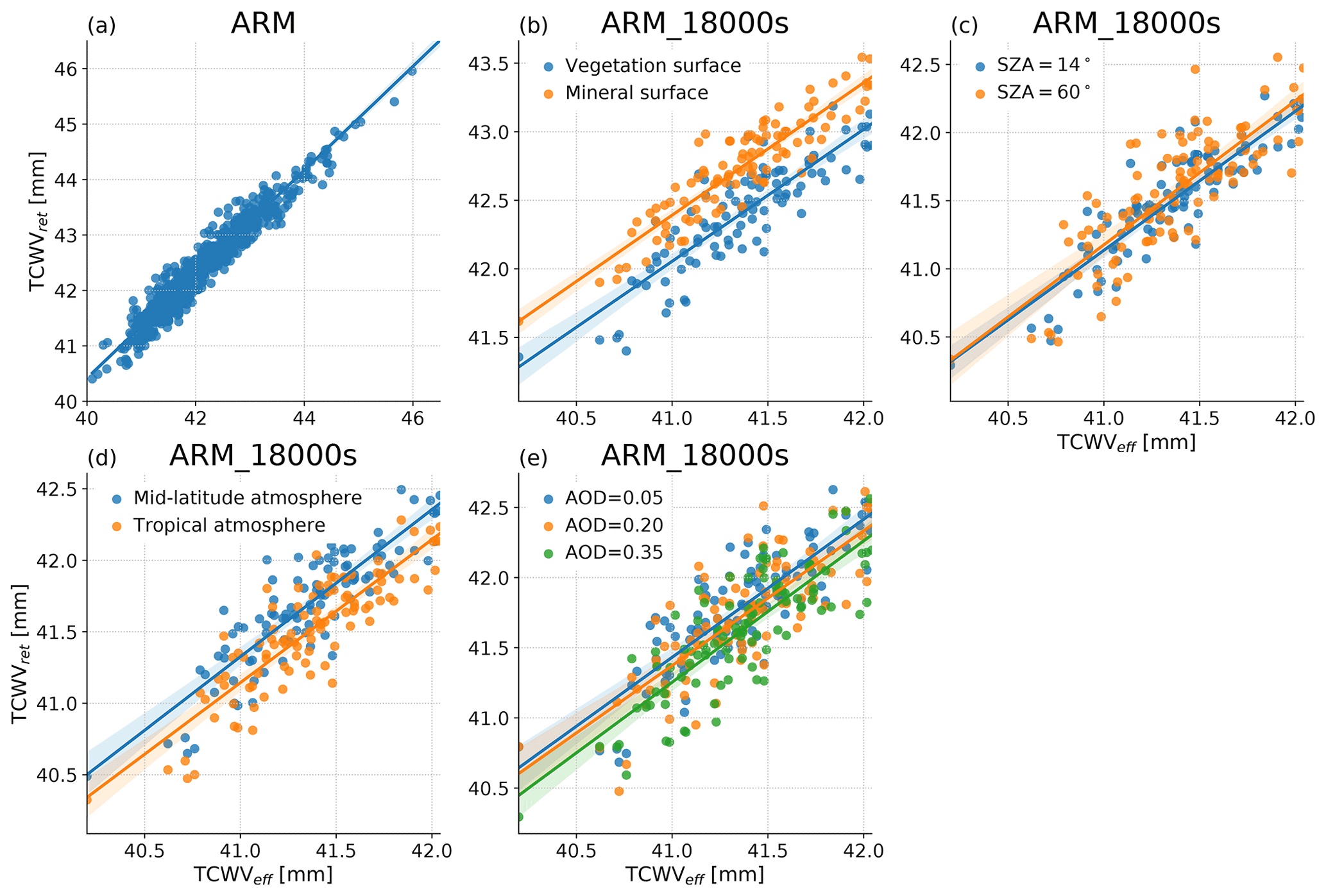
Figure 2TCWVret as a function of TCWV along with emulator fits: (a) for subsets from all ARM snapshots with SZA = 45∘ over a cropland surface. (b) Over two typical different surfaces, ARM_18000s only, (c) with different SZAs, (d) when changing a retrieval's assumed q(z) and T(z), and (e) when changing AOD.
Figure 2a shows the linear relationship from all ARM snapshots, while Fig. 2b–e show how the parameters may vary with surface type, SZA, retrieval-assumed atmospheric profile shapes, and AOD.
Figure 2b shows that a2 varies between a vegetation surface and a mineral surface. Surface type can vary greatly on sub-kilometre scales, and within-scene transitions between vegetation and mineral surfaces would introduce artificial variance in TCWVret differences either side of transition boundaries and potentially affect the derived S2 and ζ2. Variations in a2 are small when considering mixtures of vegetation or mixtures of urban-mineral surfaces, so we limit our structure-function analysis to mixed-vegetation or urban-mineral surfaces.
From Fig. 2c, TCWVret is only weakly sensitive to SZA from 14 to 60∘, the derived parameters do not differ significantly, and for SZA from 14 to 45∘ TCWVret are extremely similar. From this we argue that we can use a single set of derived parameters for each LES case for SZA up to 60∘.
Next, we note that absorption line broadening depends on thermodynamics and so argue that the structure of q(z) can change a1 and a2. For example, changes in q at a lower, warmer level will result in stronger changes in absorption at the edges of bands compared with changes in q at a higher, cooler level. Figure 2d presents results from one test that support this argument, when the atmosphere used in the retrieval's LUT is changed from mid-latitude summer to tropical and the parameters change. Similarly, substantial changes in the forward model q(z) profiles change the derived parameters (not shown). We note that Fig. 2a contains results from different LES time steps in which the atmospheric profiles evolved, but this evolution was too small to generate any detectable differences in the Eq. (8) parameters.
Finally, we considered the relationship between AOD and the parameters in Eq. (8). In all other panels AOD varied randomly from 0.1 to 0.2 between footprints, but in Fig. 2e the simulations are performed with AOD fixed across all footprints at either 0.05, 0.20, or 0.35. Changing AOD by 0.3 results in a change in a2 equivalent to approximately 0.3 % of TCWVeff. This is a smaller change than between common surface types (Fig. 2b), and AOD varies far more smoothly at sub-kilometre horizontal scales than surface type, so we anticipated that our results would be robust to some types of spatial aerosol variability. In Sect. 3.2 we show how vertical gradients of up to 0.3 AOD km−1 can have a minor effect on derived exponents.
2.2.2 Generating retrieved fields
For SZA from 0 to 60∘ in increments of 15∘, the PIWV was calculated by ray tracing from the top of the atmosphere to centre of each surface grid cell and then directly up with a solar azimuth of 0∘. This geometry represents a nadir instrument view angle, and PIWV is then converted to TCWVeff via Eq. (7), which accounts for SZA. This TCWVeff is then used as input for Eq. (8), thereby generating TCWVret fields for analysis.
As mentioned in Sect. 2.2.1, each separate LES case has a unique set of Eq. (8) parameters, and the fit is generated from plane-parallel radiative transfer calculations. This means that horizontal variability in q is not explicitly accounted for, but we argue that the derivation includes a range of q(z) profiles, and there is no fundamental reason why should introduce fundamental differences that should affect our Eq. (8) relationship. Therefore, we assume that the relationship between TCWVret and PIWV will be captured by Eq. (4).
The same ray-traced calculation is repeated with cloud water qc to obtain cloud water path (CWP). Footprints are then flagged as cloudy or shaded when CWP > 1 × 10⁻³ mm for any of the selected SZAs so as to avoid changes in ζ2 due to changes in the footprints considered. This CWP is equivalent to approximately τ > 0.3 in a typical sub-adiabatic cloud (Szczodrak et al., 2001).
2.3 Calculation of spatial statistics and removal of random error
S2(r) is calculated from the LES field of TCWVret in one horizontal direction at a time by including all pairs of footprints separated by r in that direction provided that neither of the footprints in the pair is flagged as cloudy or shadowed for any SZA. To calculate along the LES x axis, each different y location is effectively treated as a 1-D field and its set of values is calculated, and then all the 1-D subsets are concatenated and the reported S2(r) is the expectation value of this combined dataset.
The horizontal directions are either along the x axis (“perpendicular” to the sunlight) or along the y axis (the “parallel” case). Figure 3 displays example S2(r) for clear-sky TCWV and their associated scaling parameters, i.e. , showing that ζ2 will depend on the range of r over which it is calculated. The variation of ζ2 with Δr can be due to changes in physical processes in addition to imperfect process representation in the LES, such as non-physical dissipation at separations smaller than several grid cells (Brown et al., 2002). This study is not concerned with the interpretation of ζ2 but rather with the accuracy with which it can be obtained, so we do not explore this further and follow Thompson et al. (2021) in calculating the fit over r=0.5–1 km.
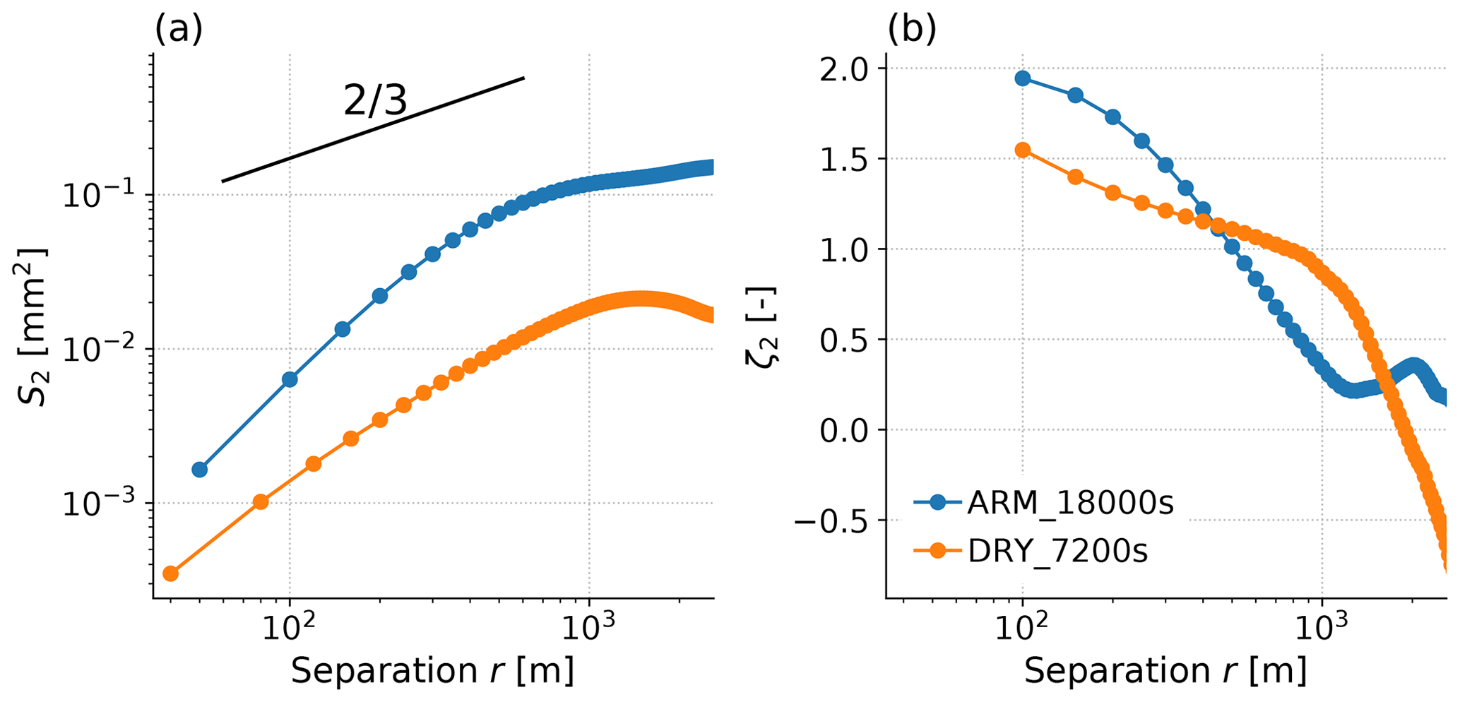
Figure 3(a) S2 calculated from TCWV for two LES snapshots as a function of separation distance, with the gradient associated with a passive tracer in turbulence following Kolmogorov theory also shown; (b) exponent calculated locally at each separation distance.
We estimate and remove the measurement noise following the method of Richardson et al. (2021a). They derived a structure-function-based method to estimate σε from the TCWVret field, thereby allowing better estimation of S2 by subtracting from Eq. (5). This method involves calculating S2 in one horizontal direction at r=Δx (i.e. separation of one grid cell, 40 or 50 m) and then smoothing the field by a factor of 2 in the perpendicular direction and recalculating S2, which we label . At these small separations, , such that .
We evaluate the sensitivity of our derived ζ2 to uncertainty in the retrieval emulator; when calculating S2 from the retrieved fields, the emulator changes the retrieved value S2,ret to
and the estimated ζ2,ret is
This shows that both biases in a1 (“retrieval sensitivity”) and the magnitude of random errors can change the derived ζ2. Richardson et al. (2021a) showed that errors in a1 were the largest source of uncertainty in estimating the spatial standard deviation. We will therefore perform sensitivity tests for a range of a1 values and show only one σε case since results were insensitive to changes in σε of up to a factor of 4 scaling.
The final question we address is whether the scaling exponent estimated at the very high spatial resolution of missions such as EMIT will be fundamentally different from that obtained by current sensors such as MERIS and MODIS that can provide TCWV at a nominal resolution near Δx≈250 m. Large-scale σx narrows as spatial resolution coarsens, but it is not clear how this affects the spatial scaling properties considered here, so for this test we sequentially degrade a TCWV field from Δx=50 m to Δx=250 m and calculate S2 and ζ2 at each resolution.
3.1 Variation of horizontal ζ2 with height
Figure 4 shows how the ζ2 calculated for PCWV integrated up to different heights varies within the PBL but that the value becomes fixed by the PBL top. That is, estimates made from TCWV refer to the value for PCWVPBL, but this conceals vertical structure within the PBL. We can therefore confirm that our derived values are indeed representative of ζ2 derived from PCWVPBL, but further work is needed to determine the precise utility of statistics of PCWVPBL and, furthermore, we note that corresponding estimates of PBL height from other sources may be necessary to help interpret measurements of PCWVPBL scaling.
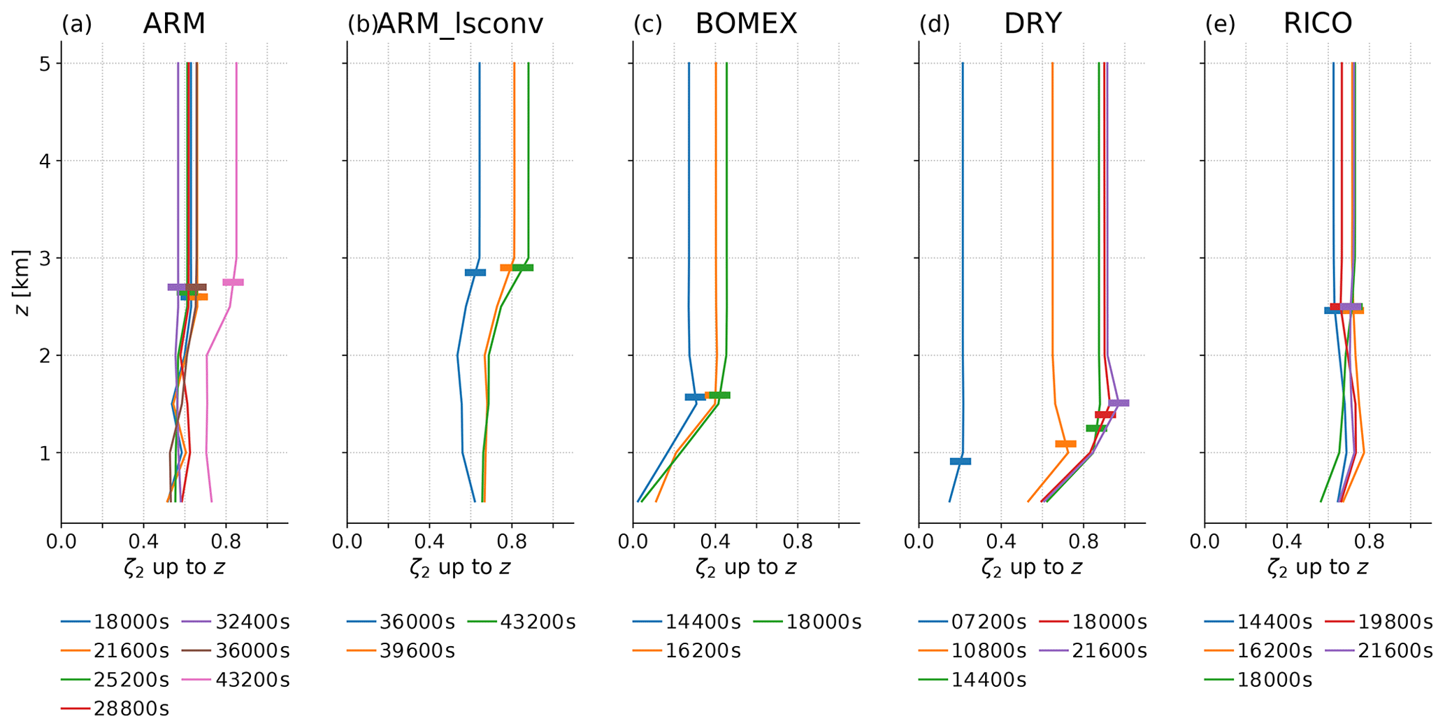
Figure 4Calculated structure function exponents using separation distance 0.5–1 km directly on LES output, calculated for integrated water vapour up to each labelled capping altitude, every 0.5 km. The PBL top derived from the location of the maximum vertical gradient in potential temperature is shown as a horizontal bar for each profile.
3.2 Retrieval errors and ζ2
The results from all sensitivity tests applied to the clear-sky TCWV in the ARM_18000s snapshot are shown in Fig. 5; results are similar for other snapshots (not shown). Figure 3a shows that random errors that we estimate will be typical for EMIT and result in substantial changes to calculated , with a notable flattening over much of the r range and an unacceptably large error in ζ2 derived from retrieved TCWV. Our error correction reduces the ζ2 error from 53.1 % to 1.4 %. Figure 5b shows that errors in the sensitivity , which is the emulator parameter a1 in Eq. (8), shift S2 but do not substantially affect the gradient over r=0.5–1 km, and this conclusion also applies in Fig. 5c when biases in a1 are combined with σε and the error correction is applied. These results show that even large biases in a1, which contribute proportionally to estimates of errors in σx, do not have a substantial effect on derived scaling properties.
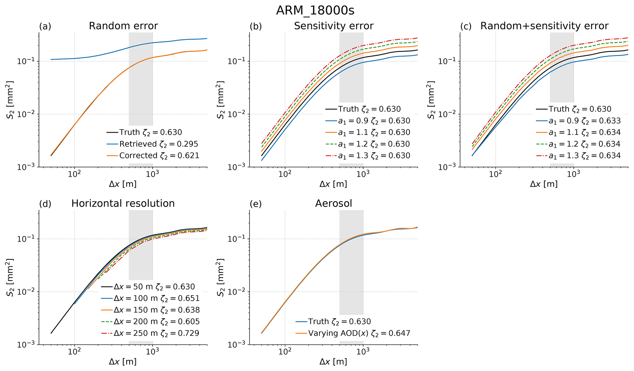
Figure 5Sensitivity of derived S2 to retrieval errors and spatial resolution; the legends in each case report the calculated exponent from a fit over separations 0.5–1 km, the region which is shaded grey in each panel. In each case “truth” refers to the value calculated from TCWV at a native LES resolution of 50 m. (a) Blue shows S2 derived from retrieved TCWV including random error only, and orange the S2 after subtracting the estimated retrieval variance. (b) S2 calculated with no random error but non-unity sensitivity as defined by the a1 trend parameter in Eq. (8). (c) The result when combining random error and sensitivity error, after subtraction of the random error estimated from each retrieved field. (d) S2 calculated after smoothing the field resolution sequentially to 250 m × 250 m. (e) S2 calculated for a horizontally varying aerosol field where TCWVret changes sinusoidally by 0.3 % every 1 km, representing a change of 0.3 in AOD based on the TCWVret response from Fig. 1e.
Figure 5d confirms that scaling properties are sensitive to the measurement resolution, with derived exponents varying unpredictably from 0.61 to 0.73 with resolution. For Δx=250 m there are only five points included in the regression. Furthermore, more footprints will be partially cloudy, meaning that the samples included will be too small for robust estimation of ζ2. We did not apply a matched cloud mask for this test and expect that this will lead to more uncertain estimates of ζ2. Tests across all 23 snapshots show that most return a higher, and more uncertain, ζ2 when spatial resolution is degraded (not shown). This points to new information being obtained from finer-spatial-resolution retrievals provided that the slanted solar paths do not destroy the correspondence between true and retrieved ζ2.
The final panel, Fig. 5e, shows a sensitivity test to strong spatial gradients in AOD. From Fig. 2e, a change of 0.3 in AOD results in a difference of 0.3 % in TCWVret in ARM_18000s, and other tests found a smaller fractional response in DRY_7200s (not shown). We picked the ARM_18000s results as the worst case and allowed TCWVret to vary sinusoidally in the x direction by ±0.15 % with a wavelength of 2 km. This approximates the effect of a change of approximately 0.3 AOD every 1 km. This relatively extreme AOD gradient changes ζ2 by < 4 % in all cases except DRY (not shown). In the DRY LES run our aerosol gradients induce a factor of 2 change in time step DRY_7200s and 10 % in other time steps. This larger relative error may be related to their small spatial variability of TCWV and low values of ζ2.
This test represents a very large horizontal change in AOD, and since ISOFIT simultaneously retrieves AOD, such cases could be identified. Overall, we conclude that for scenes where AOD is of order 0.35 or less and horizontal gradients are smaller than 0.3 AOD km−1, our results will generally be robust to typical aerosol variability. In practice, we would recommend testing each case using coincidentally retrieved AOD fields along with the estimated sensitivity of TCWVret to AOD to calculate a likely effect of special AOD variability. This may identify cases where aerosol variability affects derived ζ2.
3.3 Solar zenith angle, calculation direction, and ζ2
In our final tests we compare ζ2 calculated on the TCWVret fields with SZA changed from 15 to 60∘ as a function of the “true” value obtained from the TCWV field. The TCWVret values are those using each simulation's emulator parameters and include the random error correction, while the true values refer to the columns directly over each footprint with no retrieval error. All use Δx=40–50 m with fits calculated over r=500–1000 m, and calculations are either along the y axis and parallel to the solar azimuth or along the x axis and perpendicular to the solar azimuth.
Figure 6 shows that there is substantial spread introduced for realistic SZA, with a strong tendency for bias in ζ2 to increase with SZA when calculated parallel to the solar azimuth. This spread and apparent bias are greatly reduced when the calculation is performed perpendicularly to the solar azimuth. In the parallel case there are still significant differences (p < 0.05) between true and retrieved ζ2. The p=0.05 value threshold is calculated as 1.96 times the standard error of the difference in best-fit parameters derived from the ln (S2) as a function of ln (r) gradient.
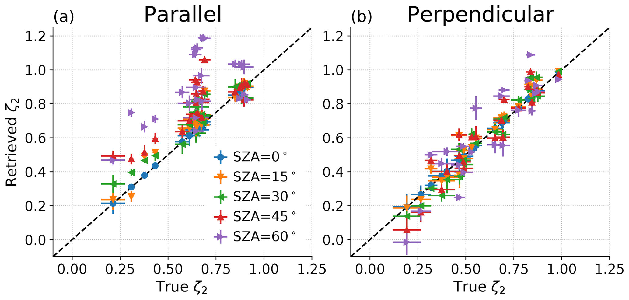
Figure 6Estimated clear-sky ζ2 over separations 0.5–1 km in all 23 snapshots as a function of the true value. The error bars are ±2σ from the trend fit.
Figure 7 shows that both bias and error range expand with SZA when calculating in the solar azimuth direction, but the median (and mean, not shown) bias is eliminated by calculating S2 in the direction perpendicular to the solar azimuth. The spread is also wider in the parallel case, the 5 %–95 % range of differences relative to the truth is −0.04–0.49 versus −0.20–0.22 when calculating perpendicular, while the standard deviation is 0.18 for parallel versus 0.13 for perpendicular.
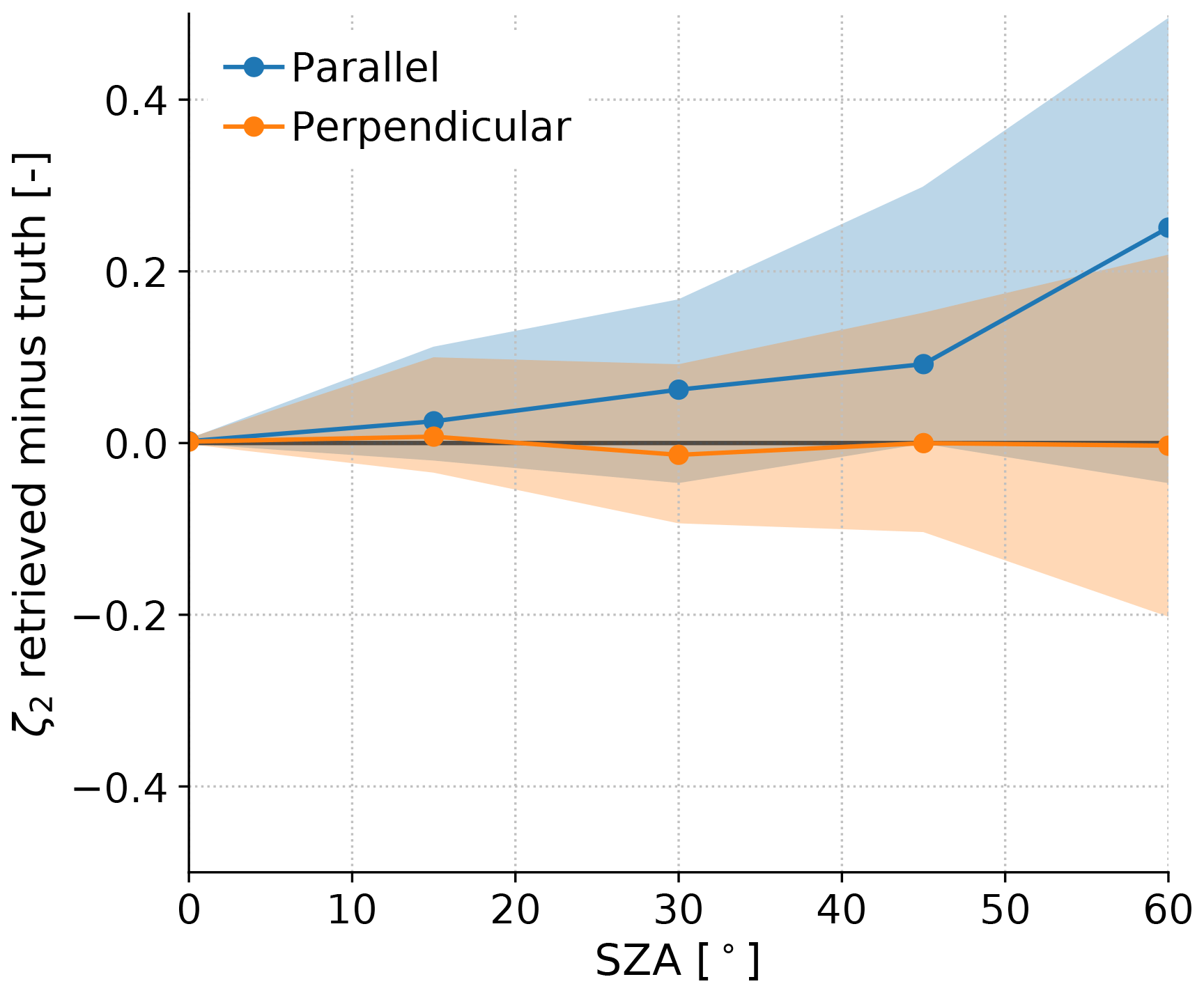
Figure 7Median and 5 %–95 % range of retrieved minus true ζ2 as a function of solar zenith angle. “Parallel” refers to calculation along the solar azimuth direction, and “Perpendicular” refers to calculation perpendicular to it.
These results show that realistic SZAs result in path-integrated water vapour structures that have somewhat different characteristics at a 0.5–1 km scale than that of the PCWVPBL over each footprint. This results in additional error to estimated ζ2, but appropriate calculation strategies that account for solar azimuth angle can reduce the magnitude of this error and suppress systematic error.
We have shown that for the q fields simulated in five LES runs of shallow convective PBLs, a novel strategy accounting for solar azimuth eliminates the SZA-induced bias in calculated ζ2 over r of 0.5–1 km from high-spatial-resolution VSWIR retrievals. This substantially increases the range of applicable geometries for which VSWIR retrievals can be used to estimate spatial scaling statistics. For example, in the airborne case studies of Thompson et al. (2021), only flight lines with SZA < 15∘ could be used, while our method promises unbiased estimates of sub-kilometre ζ2 for SZA up to 60∘. Removal of the bias is particularly important for applications, since q-scaling analyses using spaceborne data typically group or average over many sets of measurements (e.g. Kahn and Teixeira, 2009), and this averaging will not reduce bias in the way that it reduces RMSE. For the first time it also allows calculation of high-resolution ζ2 statistics over mid-latitude and polar areas of the globe that do not experience low solar zenith angles.
This approach should be applicable to any instrument that obtains TCWV from VSWIR with a horizontal resolution approaching 50 m, not just EMIT. Operationally, this requires sufficiently long, continuous sampling perpendicular to the solar azimuth. We have not analysed length requirements here but note that for airborne campaigns this is easily addressed on a flight-to-flight basis. For spaceborne instruments, the sampling will depend on the swath size and orbital geometry. EMIT's approximately 75 km swath (Bradley et al., 2020) spans distances larger than those considered here, and so we expect sampling to be sufficient regardless of orbital configuration. Similarly, ESA's CHIME contractor notes a 128 km swath, and similar capacities are expected for the missions that address NASA's Surface Biology and Geology (SBG) and Aerosols, Clouds, Convection and Precipitation (ACCP) designated observables. However, we note that it will be necessary to understand the implications of non-uniform footprint size- and footprint-dependent errors determined from the on-orbit instrument performance in order to increase the confidence in estimates of ζ2 from these spaceborne sensors.
Our analysis is based on the retrieval outputs of Richardson et al. (2021a), which showed how random retrieval error σε can be identified and removed from TCWVret fields by exploiting the properties of TCWV S2 at small scales. It also showed that errors in the T and q profiles assumed in the retrieval could affect retrieval sensitivity . We have shown here that to obtain ζ2 it is critical to remove the effect of σε but that while errors in a1 are the largest error source for estimates of spatial standard deviation, they do not greatly affect the derived ζ2.
Our results were only determined for areas where the surface type is composed either of mixed vegetation or mixed urban-mineral surfaces, so either a simultaneous surface classification (as provided by ISOFIT) or ancillary surface information would be required. We also identified that horizontal gradients of 0.3 AOD km−1 or less have only a small effect on derived ζ2 in most cases, and since ISOFIT simultaneously retrieves AOD, it seems likely that cases where this is not true could be identified. However, we highlight further investigation of the effect of realistic AOD structure as a useful future investigation. A major limitation of this study is that 1-D radiative transfer was used to derive the relationship between TCWV and TCWVret, while clouds can affect nearby clear-sky scenes through 3-D radiative effects. Future work could address this by using a 3-D radiative transfer code (e.g. Evans, 1998; Emde et al., 2011) as the forward model in an improved OSSE.
Ideally this sampling strategy could be field tested, and a strategy to do so would be to perform flights both parallel and perpendicular to the solar azimuth with collocated retrievals of TCWV from VSWIR and an independent instrument that is not affected by SZA, such as a differential absorption lidar (DIAL) or passive sounding instrument. The non-VSWIR instrument would allow calculation of ζ2 that is not affected by sunlight path, and the conclusions of this study would be supported if the VSWIR and non-VSWIR estimates showed good agreement for the perpendicular but not parallel flight paths. We highlight the High Altitude Lidar Observatory (Bedka et al., 2021) as a candidate sensor for such an experiment.
For science applications, it would also be necessary to identify which scenes are likely to satisfy our requirements: for example, conditions proximate to deep convection may have more substantial above-PBL variability at < 1 km scales and result in weaker correspondence between TCWV and PCWVPBL. In addition, it may be necessary to identify PBL height, which would require independent information from weather forecast models or reanalysis, in situ measurements, or other instruments. Furthermore, users would also need to consider the effect of sampling biases that may depend on cloud fraction or on the presence of non-isotropic variability in features such as horizontal convective rolls (e.g. as explored in Carbajal Henken et al., 2015). If locations commonly experience meteorological features with a preferential orientation, for example due to orography or a coastline, then this method may not adequately capture its full structure.
Finally, the interpretation of these exponents has not been considered in detail here, but future work could proceed either observationally or theoretically. For an observational study, the relationship between retrieved exponents and other properties, such as later convective initiation, could be investigated. A theoretical study would need to apply current understanding of turbulent physics to address precisely the problem of the horizontal variability of vertically averaged profiles. Further in the future, perhaps multi-angle imaging spectroscopy could provide profiling from VSWIR measurements via computed tomography, which has been demonstrated to retrieve aerosol profiles in some conditions using the Multi-Angle Imaging SpectroRadiometer (MISR) on Terra (Garay et al., 2016), and upper-tropospheric water vapour profiles from airborne measurements with the Gimballed Limb Observer for Radiance Imaging of the Atmosphere (GLORIA, Ungermann et al., 2015). We are not aware of any likely short-term space missions that would allow water vapour tomography from VSWIR retrievals at EMIT-like horizontal resolution, with the upcoming Multiangle Imager for Aerosols (MAIA, Diner et al., 2018) having a horizontal resolution similar to that of MODIS. If such an instrument were launched, high-spatial-resolution tomography would also be subject to the smearing effect from the non-vertical solar path and so may benefit from our proposal, although a detailed study of the particular instrument and retrieval set-up would be required.
Our main conclusion is that a novel sampling strategy can allow a breakthrough in space-based measurement of PBL water vapour scaling and that while individual uncertainties and geographical sampling may vary with the mission, this principle will apply to the array of upcoming VSWIR instruments whose spectra will allow column water vapour retrievals at resolutions from 30 to 80 m or better. The resulting statistics offer a new check on the validity of high-resolution atmospheric models and inform sub-grid parameterisations of coarser ESMs.
The MODTRAN radiative transfer code is available at http://modtran.spectral.com/, licence required, last access: 19 March 2020, Berk et al., 2014, 2015) and requires a licence. The LES profiles used in the emulator development and the 2-D LES output fields used in this analysis are available at https://doi.org/10.5281/zenodo.5717263 (Richardson et al., 2021b).
The supplement related to this article is available online at: https://doi.org/10.5194/amt-15-117-2022-supplement.
MTR processed the data and generated the figures. DRT developed the retrieval code (Isofit) used to generate the retrieval emulators. MJK generated and provided the large eddy simulation output. MDL initialised the project and worked with MTR on analysis design and data interpretation. All the authors contributed to the conceptualisation, writing, and editing.
The contact author has declared that neither they nor their co-authors have any competing interests.
Publisher’s note: Copernicus Publications remains neutral with regard to jurisdictional claims in published maps and institutional affiliations.
This research was carried out at the Jet Propulsion Laboratory, California Institute of Technology, Pasadena, CA, USA, under contract with the National Aeronautics and Space Administration. Mark T. Richardson thanks Amin Nehrir and Brian Carroll of NASA Langley for helpful discussion regarding HALO lidar data.
This research has been supported by the National Aeronautics and Space Administration, Jet Propulsion Laboratory (grant no. 80NM0018F0631).
This paper was edited by Joanna Joiner and reviewed by Christoph Kiemle, Alexander Marshak, and one anonymous referee.
Arakawa, A., Jung, J.-H., and Wu, C.-M.: Toward unification of the multiscale modeling of the atmosphere, Atmos. Chem. Phys., 11, 3731–3742, https://doi.org/10.5194/acp-11-3731-2011, 2011.
Bacmeister, J. T., Eckermann, S. D., Newman, P. A., Lait, L., Chan, K. R., Loewenstein, M., Proffitt, M. H., and Gary, B. L.: Stratospheric horizontal wavenumber spectra of winds, potential temperature, and atmospheric tracers observed by high-altitude aircraft, J. Geophys. Res.-Atmos., 101, 9441–9470, https://doi.org/10.1029/95JD03835, 1996.
Bedka, K. M., Nehrir, A. R., Kavaya, M., Barton-Grimley, R., Beaubien, M., Carroll, B., Collins, J., Cooney, J., Emmitt, G. D., Greco, S., Kooi, S., Lee, T., Liu, Z., Rodier, S., and Skofronick-Jackson, G.: Airborne lidar observations of wind, water vapor, and aerosol profiles during the NASA Aeolus calibration and validation (Cal/Val) test flight campaign, Atmos. Meas. Tech., 14, 4305–4334, https://doi.org/10.5194/amt-14-4305-2021, 2021.
Berk, A., Conforti, P., Kennett, R., Perkins, T., Hawes, F., and van den Bosch, J.: MODTRAN6: a major upgrade of the MODTRAN radiative transfer code, in: Proceedings Volume 9088, Algorithms and Technologies for Multispectral, Hyperspectral, and Ultraspectral Imagery XX, edited by: Velez-Reyes, M. and Kruse, F. A., SPIE, Baltimore, MD, USA, 90880H, 2014.
Berk, A., Conforti, P., and Hawes, F.: An accelerated line-by-line option for MODTRAN combining on-the-fly generation of line center absorption within 0.1 cm−1 bins and pre-computed line tails, in: Proceedings Volume 9472, Algorithms and Technologies for Multispectral, Hyperspectral, and Ultraspectral Imagery XXI, edited by: Velez-Reyes, M. and Kruse, F. A., SPIE, Baltimore, MD, USA, 947217, 2015.
Boffetta, G., De Lillo, F., Mazzino, A., and Musacchio, S.: Bolgiano scale in confined Rayleigh–Taylor turbulence, J. Fluid Mech., 690, 426–440, https://doi.org/10.1017/jfm.2011.446, 2012.
Bolgiano, R.: Turbulent spectra in a stably stratified atmosphere, J. Geophys. Res., 64, 2226–2229, https://doi.org/10.1029/JZ064i012p02226, 1959.
Bradley, C. L., Thingvold, E., Moore, L. B., Haag, J. M., Raouf, N. A., Mouroulis, P., and Green, R. O.: Optical design of the Earth Surface Mineral Dust Source Investigation (EMIT) imaging spectrometer, in: Imaging Spectrometry XXIV: Applications, Sensors, and Processing, edited by: Mouroulis, P. and Ientilucci, E. J., SPIE Optical Engineering + Applications, online only, p. 1, 2020.
Brown, A. R., Cederwall, R. T., Chlond, A., Duynkerke, P. G., Golaz, J.-C., Khairoutdinov, M., Lewellen, D. C., Lock, A. P., MacVean, M. K., Moeng, C.-H., Neggers, R. A. J., Siebesma, A. P., and Stevens, B.: Large-eddy simulation of the diurnal cycle of shallow cumulus convection over land, Q. J. R. Meteorol. Soc., 128, 1075–1093, https://doi.org/10.1256/003590002320373210, 2002.
Candela, L., Formaro, R., Guarini, R., Loizzo, R., Longo, F., and Varacalli, G.: The PRISMA mission, in: 2016 IEEE International Geoscience and Remote Sensing Symposium (IGARSS), IEEE, Beijing, China, 10–15 July 2016, 253–256, 2016.
Carbajal Henken, C. K., Diedrich, H., Preusker, R., and Fischer, J.: MERIS full-resolution total column water vapor: Observing horizontal convective rolls, Geophys. Res. Lett., 42, 10074–10081, https://doi.org/10.1002/2015GL066650, 2015.
Cho, J. Y. N., Zhu, Y., Newell, R. E., Anderson, B. E., Barrick, J. D., Gregory, G. L., Sachse, G. W., Carroll, M. A., and Albercook, G. M.: Horizontal wavenumber spectra of winds, temperature, and trace gases during the Pacific Exploratory Missions: 1. Climatology, J. Geophys. Res.-Atmos., 104, 5697–5716, https://doi.org/10.1029/98JD01825, 1999.
Diedrich, H., Preusker, R., Lindstrot, R., and Fischer, J.: Retrieval of daytime total columnar water vapour from MODIS measurements over land surfaces, Atmos. Meas. Tech., 8, 823–836, https://doi.org/10.5194/amt-8-823-2015, 2015.
Diner, D. J., Boland, S. W., Brauer, M., Bruegge, C., Burke, K. A., Chipman, R., Di Girolamo, L., Garay, M. J., Hasheminassab, S., and Hyer, E.: Advances in multiangle satellite remote sensing of speciated airborne particulate matter and association with adverse health effects: from MISR to MAIA, J. Appl. Remote Sens., 16, 042603, https://doi.org/10.1117/1.JRS.12.042603, 2018.
Dorrestijn, J., Kahn, B. H., Teixeira, J., and Irion, F. W.: Instantaneous variance scaling of AIRS thermodynamic profiles using a circular area Monte Carlo approach, Atmos. Meas. Tech., 11, 2717–2733, https://doi.org/10.5194/amt-11-2717-2018, 2018.
Drusch, M., Del Bello, U., Carlier, S., Colin, O., Fernandez, V., Gascon, F., Hoersch, B., Isola, C., Laberinti, P., Martimort, P., Meygret, A., Spoto, F., Sy, O., Marchese, F., and Bargellini, P.: Sentinel-2: ESA's Optical High-Resolution Mission for GMES Operational Services, Remote Sens. Environ., 120, 25–36, https://doi.org/10.1016/j.rse.2011.11.026, 2012.
Emde, C., Buras, R., and Mayer, B.: ALIS: An efficient method to compute high spectral resolution polarized solar radiances using the Monte Carlo approach, J. Quant. Spectrosc. Radiat. Transf., 112, 1622–1631, https://doi.org/10.1016/j.jqsrt.2011.03.018, 2011.
Evans, K. F.: The Spherical Harmonics Discrete Ordinate Method for Three-Dimensional Atmospheric Radiative Transfer, J. Atmos. Sci., 55, 429–446, https://doi.org/10.1175/1520-0469(1998)055<0429:TSHDOM>2.0.CO;2, 1998.
Fischer, L., Kiemle, C., and Craig, G. C.: Height-resolved variability of midlatitude tropospheric water vapor measured by an airborne lidar, Geophys. Res. Lett., 39, L06803, https://doi.org/10.1029/2011GL050621, 2012.
Fischer, L., Craig, G. C., and Kiemle, C.: Horizontal structure function and vertical correlation analysis of mesoscale water vapor variability observed by airborne lidar, J. Geophys. Res.-Atmos., 118, 7579–7590, https://doi.org/10.1002/jgrd.50588, 2013.
Gage, K. S. and Nastrom, G. D.: On the spectrum of atmospheric velocity fluctuations seen by MST/ST radar and their interpretation, Radio Sci., 20, 1339–1347, https://doi.org/10.1029/RS020i006p01339, 1985.
Garay, M. J., Davis, A. B., and Diner, D. J.: Tomographic reconstruction of an aerosol plume using passive multiangle observations from the MISR satellite instrument, Geophys. Res. Lett., 43, 12590–12596, https://doi.org/10.1002/2016GL071479, 2016.
Gelaro, R., McCarty, W., Suárez, M. J., Todling, R., Molod, A., Takacs, L., Randles, C. A., Darmenov, A., Bosilovich, M. G., Reichle, R., Wargan, K., Coy, L., Cullather, R., Draper, C., Akella, S., Buchard, V., Conaty, A., da Silva, A. M., Gu, W., Kim, G.-K., Koster, R., Lucchesi, R., Merkova, D., Nielsen, J. E., Partyka, G., Pawson, S., Putman, W., Rienecker, M., Schubert, S. D., Sienkiewicz, M., and Zhao, B.: The Modern-Era Retrospective Analysis for Research and Applications, Version 2 (MERRA-2), J. Climate, 30, 5419–5454, https://doi.org/10.1175/JCLI-D-16-0758.1, 2017.
Golaz, J.-C., Larson, V. E., and Cotton, W. R.: A PDF-Based Model for Boundary Layer Clouds. Part I: Method and Model Description, J. Atmos. Sci., 59, 3540–3551, https://doi.org/10.1175/1520-0469(2002)059<3540:APBMFB>2.0.CO;2, 2002.
Green, R. O. and Thompson, D. R.: An Earth Science Imaging Spectroscopy Mission: The Earth Surface Mineral Dust Source Investigation (EMIT), in: IGARSS 2020 – 2020 IEEE International Geoscience and Remote Sensing Symposium, online only, 26 September–2 October 2020, IEEE, 6262–6265, 2020.
Gristey, J. J., Feingold, G., Glenn, I. B., Schmidt, K. S., and Chen, H.: Surface Solar Irradiance in Continental Shallow Cumulus Fields: Observations and Large-Eddy Simulation, J. Atmos. Sci., 77, 1065–1080, https://doi.org/10.1175/JAS-D-19-0261.1, 2019.
Grossi, M., Valks, P., Loyola, D., Aberle, B., Slijkhuis, S., Wagner, T., Beirle, S., and Lang, R.: Total column water vapour measurements from GOME-2 MetOp-A and MetOp-B, Atmos. Meas. Tech., 8, 1111–1133, https://doi.org/10.5194/amt-8-1111-2015, 2015.
Kahn, B. H. and Teixeira, J.: A Global Climatology of Temperature and Water Vapor Variance Scaling from the Atmospheric Infrared Sounder, J. Climate, 22, 5558–5576, https://doi.org/10.1175/2009JCLI2934.1, 2009.
Kahn, B. H., Teixeira, J., Fetzer, E. J., Gettelman, A., Hristova-Veleva, S. M., Huang, X., Kochanski, A. K., Köhler, M., Krueger, S. K., Wood, R., and Zhao, M.: Temperature and Water Vapor Variance Scaling in Global Models: Comparisons to Satellite and Aircraft Data, J. Atmos. Sci., 68, 2156–2168, https://doi.org/10.1175/2011JAS3737.1, 2011.
Krutz, D., Müller, R., Knodt, U., Günther, B., Walter, I., Sebastian, I., Säuberlich, T., Reulke, R., Carmona, E., Eckardt, A., Venus, H., Fischer, C., Zender, B., Arloth, S., Lieder, M., Neidhardt, M., Grote, U., Schrandt, F., Gelmi, S., and Wojtkowiak, A.: The Instrument Design of the DLR Earth Sensing Imaging Spectrometer (DESIS), Sensors, 19, 1622, https://doi.org/10.3390/s19071622, 2019.
Kunnen, R. P. J., Clercx, H. J. H., Geurts, B. J., van Bokhoven, L. J. A., Akkermans, R. A. D., and Verzicco, R.: Numerical and experimental investigation of structure-function scaling in turbulent Rayleigh-Bénard convection, Phys. Rev. E, 77, 016302, https://doi.org/10.1103/PhysRevE.77.016302, 2008.
Kurowski, M. J., Grabowski, W. W., and Smolarkiewicz, P. K.: Anelastic and Compressible Simulation of Moist Dynamics at Planetary Scales, J. Atmos. Sci., 72, 3975–3995, https://doi.org/10.1175/JAS-D-15-0107.1, 2015.
Kurowski, M. J., Grabowski, W. W., Suselj, K., and Teixeira, J.: The Strong Impact of Weak Horizontal Convergence on Continental Shallow Convection, J. Atmos. Sci., 77, 3119–3137, https://doi.org/10.1175/JAS-D-19-0351.1, 2020.
Lovejoy, S., Schertzer, D., and Tuck, A. F.: Fractal aircraft trajectories and nonclassical turbulent exponents, Phys. Rev. E, 70, 036306, https://doi.org/10.1103/PhysRevE.70.036306, 2004.
Lovejoy, S., Tuck, A. F., Hovde, S. J., and Schertzer, D.: Is isotropic turbulence relevant in the atmosphere?, Geophys. Res. Lett., 34, L15802, https://doi.org/10.1029/2007GL029359, 2007.
Massie, S. T., Cronk, H., Merrelli, A., O'Dell, C., Schmidt, K. S., Chen, H., and Baker, D.: Analysis of 3D cloud effects in OCO-2 XCO2 retrievals, Atmos. Meas. Tech., 14, 1475–1499, https://doi.org/10.5194/amt-14-1475-2021, 2021.
Matheou, G. and Chung, D.: Large-Eddy Simulation of Stratified Turbulence. Part II: Application of the Stretched-Vortex Model to the Atmospheric Boundary Layer, J. Atmos. Sci., 71, 4439–4460, https://doi.org/10.1175/JAS-D-13-0306.1, 2014.
Nelson, R. R., Crisp, D., Ott, L. E., and O'Dell, C. W.: High-accuracy measurements of total column water vapor from the Orbiting Carbon Observatory-2, Geophys. Res. Lett., 43, 12261–12269, https://doi.org/10.1002/2016GL071200, 2016.
Noël, S., Buchwitz, M., and Burrows, J. P.: First retrieval of global water vapour column amounts from SCIAMACHY measurements, Atmos. Chem. Phys., 4, 111–125, https://doi.org/10.5194/acp-4-111-2004, 2004.
Obukhov, A. M.: On the influence of buoyancy forces on the structure of the temperature field in a turbulent flow, Dokl. Acad. Nauk. SSST., 125, p. 1246, 1959.
Perraud, E., Couvreux, F., Malardel, S., Lac, C., Masson, V., and Thouron, O.: Evaluation of Statistical Distributions for the Parametrization of Subgrid Boundary-Layer Clouds, Bound.-Lay. Meteorol., 140, 263–294, https://doi.org/10.1007/s10546-011-9607-3, 2011.
Pinel, J., Lovejoy, S., Schertzer, D., and Tuck, A. F.: Joint horizontal-vertical anisotropic scaling, isobaric and isoheight wind statistics from aircraft data, Geophys. Res. Lett., 39, L11803, https://doi.org/10.1029/2012GL051689, 2012.
Pressel, K. G. and Collins, W. D.: First-Order Structure Function Analysis of Statistical Scale Invariance in the AIRS-Observed Water Vapor Field, J. Climate, 25, 5538–5555, https://doi.org/10.1175/JCLI-D-11-00374.1, 2012.
Preusker, R., Carbajal Henken, C., and Fischer, J.: Retrieval of Daytime Total Column Water Vapour from OLCI Measurements over Land Surfaces, Remote Sens., 13, 932, https://doi.org/10.3390/rs13050932, 2021.
Prusa, J. M., Smolarkiewicz, P. K., and Wyszogrodzki, A. A.: EULAG, a computational model for multiscale flows, Comput. Fluids, 37, 1193–1207, https://doi.org/10.1016/j.compfluid.2007.12.001, 2008.
Rast, M., Ananasso, C., Bach, H., Ben-Dor, E., Chabrillat, S., Colombo, R., Del Bello, U., Feret, J., Giardino, C., Green, R., Guanter, L., Marsh, S., Nieke, J., CCH, O., Rum, G., Schaepman, M., Schlerf, M., Skidmore, A., and Strobl, P.: Copernicus hyperspectral imaging mission for the environment: Mission requirements document version 2.1, European Space Agency, Frascati, Italy, 2019.
Richardson, M. T., Thompson, D. R., Kurowski, M. J., and Lebsock, M. D.: Boundary layer water vapour statistics from high-spatial-resolution spaceborne imaging spectroscopy, Atmos. Meas. Tech., 14, 5555–5576, https://doi.org/10.5194/amt-14-5555-2021, 2021a.
Richardson, M. T., Thompson, D. R., Kurowski, M. J., and Lebsock, M. D.: Supporting data for boundary layer water vapour statistics from high-spatial-resolution spaceborne imaging spectroscopy, Zenodo [data set], https://doi.org/10.5281/zenodo.5717263, 2021b.
Schemann, V., Stevens, B., Grützun, V., and Quaas, J.: Scale Dependency of Total Water Variance and Its Implication for Cloud Parameterizations, J. Atmos. Sci., 70, 3615–3630, https://doi.org/10.1175/JAS-D-13-09.1, 2013.
Selz, T., Fischer, L., and Craig, G. C.: Structure Function Analysis of Water Vapor Simulated with a Convection-Permitting Model and Comparison to Airborne Lidar Observations, J. Atmos. Sci., 74, 1201–1210, https://doi.org/10.1175/JAS-D-16-0160.1, 2017.
Siebesma, A. P., Bretherton, C. S., Brown, A., Chlond, A., Cuxart, J., Duynkerke, P. G., Jiang, H., Khairoutdinov, M., Lewellen, D., Moeng, C.-H., Sanchez, E., Stevens, B., and Stevens, D. E.: A Large Eddy Simulation Intercomparison Study of Shallow Cumulus Convection, J. Atmos. Sci., 60, 1201–1219, https://doi.org/10.1175/1520-0469(2003)60<1201:ALESIS>2.0.CO;2, 2003.
Skamarock, W. C., Park, S.-H., Klemp, J. B., and Snyder, C.: Atmospheric Kinetic Energy Spectra from Global High-Resolution Nonhydrostatic Simulations, J. Atmos. Sci., 71, 4369–4381, https://doi.org/10.1175/JAS-D-14-0114.1, 2014.
Sommeria, G. and Deardorff, J. W.: Subgrid-Scale Condensation in Models of Nonprecipitating Clouds, J. Atmos. Sci., 34, 344–355, https://doi.org/10.1175/1520-0469(1977)034<0344:SSCIMO>2.0.CO;2, 1977.
Szczodrak, M., Austin, P. H., and Krummel, P. B.: Variability of Optical Depth and Effective Radius in Marine Stratocumulus Clouds, J. Atmos. Sci., 58, 2912–2926, https://doi.org/10.1175/1520-0469(2001)058<2912:VOODAE>2.0.CO;2, 2001.
Thompson, D. R., Natraj, V., Green, R. O., Helmlinger, M. C., Gao, B.-C., and Eastwood, M. L.: Optimal estimation for imaging spectrometer atmospheric correction, Remote Sens. Environ., 216, 355–373, https://doi.org/10.1016/j.rse.2018.07.003, 2018.
Thompson, D. R., Cawse-Nicholson, K., Erickson, Z., Fichot, C. G., Frankenberg, C., Gao, B.-C., Gierach, M. M., Green, R. O., Jensen, D., Natraj, V., and Thompson, A.: A unified approach to estimate land and water reflectances with uncertainties for coastal imaging spectroscopy, Remote Sens. Environ., 231, 111198, https://doi.org/10.1016/j.rse.2019.05.017, 2019.
Thompson, D. R., Kahn, B. H., Brodrick, P. G., Lebsock, M. D., Richardson, M., and Green, R. O.: Spectroscopic imaging of sub-kilometer spatial structure in lower-tropospheric water vapor, Atmos. Meas. Tech., 14, 2827–2840, https://doi.org/10.5194/amt-14-2827-2021, 2021.
Ungermann, J., Blank, J., Dick, M., Ebersoldt, A., Friedl-Vallon, F., Giez, A., Guggenmoser, T., Höpfner, M., Jurkat, T., Kaufmann, M., Kaufmann, S., Kleinert, A., Krämer, M., Latzko, T., Oelhaf, H., Olchewski, F., Preusse, P., Rolf, C., Schillings, J., Suminska-Ebersoldt, O., Tan, V., Thomas, N., Voigt, C., Zahn, A., Zöger, M., and Riese, M.: Level 2 processing for the imaging Fourier transform spectrometer GLORIA: derivation and validation of temperature and trace gas volume mixing ratios from calibrated dynamics mode spectra, Atmos. Meas. Tech., 8, 2473–2489, https://doi.org/10.5194/amt-8-2473-2015, 2015.
vanZanten, M. C., Stevens, B., Nuijens, L., Siebesma, A. P., Ackerman, A. S., Burnet, F., Cheng, A., Couvreux, F., Jiang, H., Khairoutdinov, M., Kogan, Y., Lewellen, D. C., Mechem, D., Nakamura, K., Noda, A., Shipway, B. J., Slawinska, J., Wang, S., and Wyszogrodzki, A.: Controls on precipitation and cloudiness in simulations of trade-wind cumulus as observed during RICO, J. Adv. Model. Earth Syst., 3, M06001, https://doi.org/10.1029/2011MS000056, 2011.
Várnai, T. and Marshak, A.: MODIS observations of enhanced clear sky reflectance near clouds, Geophys. Res. Lett., 36, L06807, https://doi.org/10.1029/2008GL037089, 2009.
Wroblewski, D. E., Coté, O. R., Hacker, J. M., and Dobosy, R. J.: Velocity and Temperature Structure Functions in the Upper Troposphere and Lower Stratosphere from High-Resolution Aircraft Measurements, J. Atmos. Sci., 67, 1157–1170, https://doi.org/10.1175/2009JAS3108.1, 2010.
smears2-D maps of imaging spectroscopy vapour retrievals. In simulations we show how this smearing is
towardsor
away fromthe Sun, so calculating
across the solar direction allows sub-kilometre information about water vapour's spatial scaling to be calculated. This could be tested by airborne campaigns and used to obtain new information from upcoming spaceborne data products.