the Creative Commons Attribution 4.0 License.
the Creative Commons Attribution 4.0 License.
 | 09 Mar 2022
A semi-automated procedure for the emitter–receiver geometry characterization of motor-controlled lidars
Marco Di Paolantonio
Davide Dionisi
Gian Luigi Liberti
To correctly understand and interpret lidar-acquired signals and to provide high-quality data, the characterization of the lidar transmitter–receiver geometry is required. For example, being fundamental to correctly align lidar systems, this characterization is useful to improve the efficiency of the alignment procedure. In addition, some applications (e.g. air quality monitoring) need to quantitatively interpret the observations even in the range where the overlap between the telescope field of view and the laser beam is incomplete. This is generally accomplished by correcting for the overlap function. Within the frame of lidar-based networks (e.g. ACTRIS/EARLINET, the Aerosol, Clouds and Trace Gases Research Infrastructure/European Aerosol Research Lidar Network), there is a need to define standardized approaches to deal with lidar geometry issues. The multi-wavelength multi-telescope Rayleigh–Mie–Raman “9-eyes” system in Rome Tor Vergata, part of ACTRIS/EARLINET, has the capability, through computer-controlled servomotors, to change the orientation of the laser beams and the 3D position of the diaphragm of the receiving optical system around the focal point of the telescopes. Taking advantage of these instrumental design characteristics an original approach to characterize the dependency of the acquired signal from the system relative transmitter–receiver geometry (the mapping procedure) was developed. The procedure consists in a set of programs controlling both the signal acquisition as well as the motor movements. The approach includes solutions to account for atmospheric and laser power variability likely to occur during the mapping sessions. The paper describes in detail the developed procedure and applications such as the optimization of the telescope/beam alignment and the estimation of the overlap function. The results of the mapping applied to a single combination of telescope-laser beam are shown and discussed. The effectiveness of the mapping-based alignment was successfully verified by comparing the whole signal profile and the outcome of the telecover test, adopted in EARLINET, for a manual and a mapping-based alignment. A significant signal increase and lowering of the full overlap height (from 1500 m to less than 1000 m) was found. The overlap function was estimated down to 200 m and compared against the one obtained from a geometric model. The developed procedure also allowed estimating the absolute and relative tilt of the laser beam. The mapping approach, even in simplified versions, can be adapted to other lidars to characterize and align systems with non-motorized receiving geometry.
- Article
(2879 KB) - Full-text XML
- BibTeX
- EndNote


Lidar (light detection and ranging) techniques are an efficient tool to provide quantitative information about vertical properties in the atmosphere (Measures, 1984; Weitkamp, 2005). Thanks to the technological advancement of the last 20 years, the employment of lidar systems in sensing the Earth atmosphere has rapidly grown. As an example, aerosol properties are studied by spaceborne lidar observations (e.g. Winker et al., 2003; McGill et al., 2015; AEOLUS), by ground-based lidar networks (e.g. the European Aerosol Research Lidar Network, EARLINET, Pappalardo et al., 2014), and, recently, by single-channel automated lidar ceilometers (e.g. Wiegner et al., 2014; Dionisi et al., 2018). In particular, the advanced multi-wavelength elastic and Raman lidars, which are part of EARLINET, provide unsurpassed information for the characterization of aerosol optical properties. This network is now a key component of ACTRIS (the Aerosol, Clouds and Trace Gases Research Infrastructure, https://www.actris.eu/, last access: 28 February 2022), a research infrastructure that will coordinate the atmospheric composition observations in Europe. Within this frame, to provide quality-assured data sets by non-standardized lidar systems, like most of those that are part of EARLINET, one of the major efforts of this community was to establish quality assurance (QA) methodologies (Pappalardo et al., 2014; Wandinger et al., 2016; Freudenthaler et al., 2018). The expected outcome of this effort is to characterize lidar performances and check, homogenize, and attest to the quality of the acquired data. After passing the QA tests, lidar raw data can then be processed by the Single Calculus Chain (SCC) that allows the “automatization and fully traceability of quality-assured aerosol optical products” (D'Amico et al., 2015). Within this frame, the characterization of lidar transmitter–receiver geometry (e.g. Halldórsson and Langerholc, 1978; Measures, 1984; Kokkalis, 2017) is essential to provide high-quality data.
As the main objective of EARLINET is the study of the aerosol in the troposphere and boundary layer (PBL), it is important to correctly interpret the received lidar signal in the lowermost range. However, bi-axial lidar systems present an incomplete response in the near-range observational field due to the partial overlap of the receiver field of view (FOV) and the transmitted beam. Therefore, to use data from heights below the full overlap height, lidar signal profiles must be corrected for this near-field loss of signal that is the overlap function O(R) (Wandinger and Ansmann, 2002), which depends on the lidar system (e.g. Wandinger et al., 2016).
Within EARLINET, the telecover test, presented by Freudenthaler et al. (2018), is a useful and easily implementable tool for the evaluation of the correct alignment of the lidar system. This method allows identifying the lower height at which the lidar signal can be used to retrieve aerosol optical properties (i.e. the lower height of full overlap for ideal lidar system); however, it cannot provide an estimation of the overlap function. In the literature various methods were developed to compute this function both analytically and experimentally. Analytical methods (e.g. Halldórsson and Langerholc, 1978; Jenness et al., 1997; Chourdakis et al., 2002; Stelmaszczyk et al., 2005; Comeron et al., 2011) require knowledge of light distribution in the laser beam cross section, receiver characteristics and relative inclination of the laser beam with respect to the receiver axis. Experimental methods on the other hand make specific assumptions or have special requirements based on the method: clear air and homogeneous aerosol distribution (Sasano et al., 1979), statistically homogeneous distribution (Tomine et al., 1989), extrapolation via polynomial regression (Dho et al., 1997), a second profile with lower overlap (e.g. ceilometer, Guerrero-Rascado et al., 2010; Sicard et al., 2020), or a Raman channel with the assumption of similar receiver geometrical configuration (Wandinger and Ansmann, 2002).
The multi-wavelength multi-telescope Rayleigh–Mie–Raman (RMR) “9-eyes” system in Rome Tor Vergata (Congeduti et al., 1999) is an old-style powerful lidar developed in the mid-90s with the objective of monitoring the mid and upper atmosphere (D'Aulerio et al., 2005; Campanelli et al., 2012; Dionisi et al., 2013a, b). To meet the EARLINET requirements, which the system has been part of since July 2016, in addition to the standard EARLINET procedure, specific tests, based on the characteristics of the system, were developed to characterize the RMR performance in the near range.
The RMR system was designed with the capability to control, through computer-controlled servomotors, the orientation of the laser beams and the 3D position of the diaphragm of the receiving optical system around the focal point of the telescopes. These instrumental characteristics were exploited to develop the mapping procedure: a set of semi-automated tools to characterize the dependency of the acquired signal from the relative transmitter–receiver geometry.
With respect to the existing approaches, the obtained results do not need any assumptions or external information and include all artefacts due to the system that may be difficult to account for in an analytical or numerical representation.
With the objective of optimizing the RMR observational performances in the troposphere and in the PBL, the developed procedure and two examples of applications are presented in this study:
-
alignment optimization based on mapping information;
-
experimental estimation of the overlap function O(R).
In Sect. 2 the relevant instrumental characteristics of the RMR lidar system with a specific focus on the emitter–receiver geometry of the system are presented. Section 3 describes the developed methodology and reports examples of telescope and laser mapping. Section 4 presents the results obtained for two applications limited to a single wavelength telescope combination. The mapping-based alignment is verified through the comparison with telecover test results. The overlap estimation is compared to the full overlap height estimated with the telecover test and with the predicted values using a simple geometric model based on the nominal characteristic of the system as presented in Sect. 2.
Finally, Sect. 5 contains the summary of the developed approach, the achieved main results, and short-term perspectives in terms of potential development. The applicability of the proposed approach to other systems is also discussed.
The design of the multi-channel multi-telescope RMR 9-eyes lidar was first presented by Congeduti et al. (1999). Since 2002 the system has been operating in the Tor Vergata experimental field in a semi-urban area southeast of Rome (41.8422∘ N, 12.6474∘ E; 107 m a.s.l.). Its current configuration is described in detail by Dionisi et al. (2010).
Here the relevant characteristics of the lidar system with an emphasis on the geometry of the emitting/receiving components are presented.
The lidar transmitter is based on a Nd:YAG laser (Continuum Powerlite 8010) with second (532 nm: green) and third (355 nm: UV) harmonic generators. The energy output is optimized for the exploitation of the UV Raman scattering. Backscattered radiation is collected and analysed at four wavelengths of interest: 532 and 355 nm for the elastic backscattering and 386.7 and 407.5 nm for Raman scattering of N2 and H2O molecules, respectively. The characteristics of the transmitted beam are reported in Table 1. In particular, it is noteworthy that the 355 and 532 nm beams are collimated by means of 5× beam expanders, and, then, they are vertically projected into the atmosphere through two 45∘ mirrors that can be azimuth- and zenith-oriented through computer-controlled servomotors (Fig. 1).
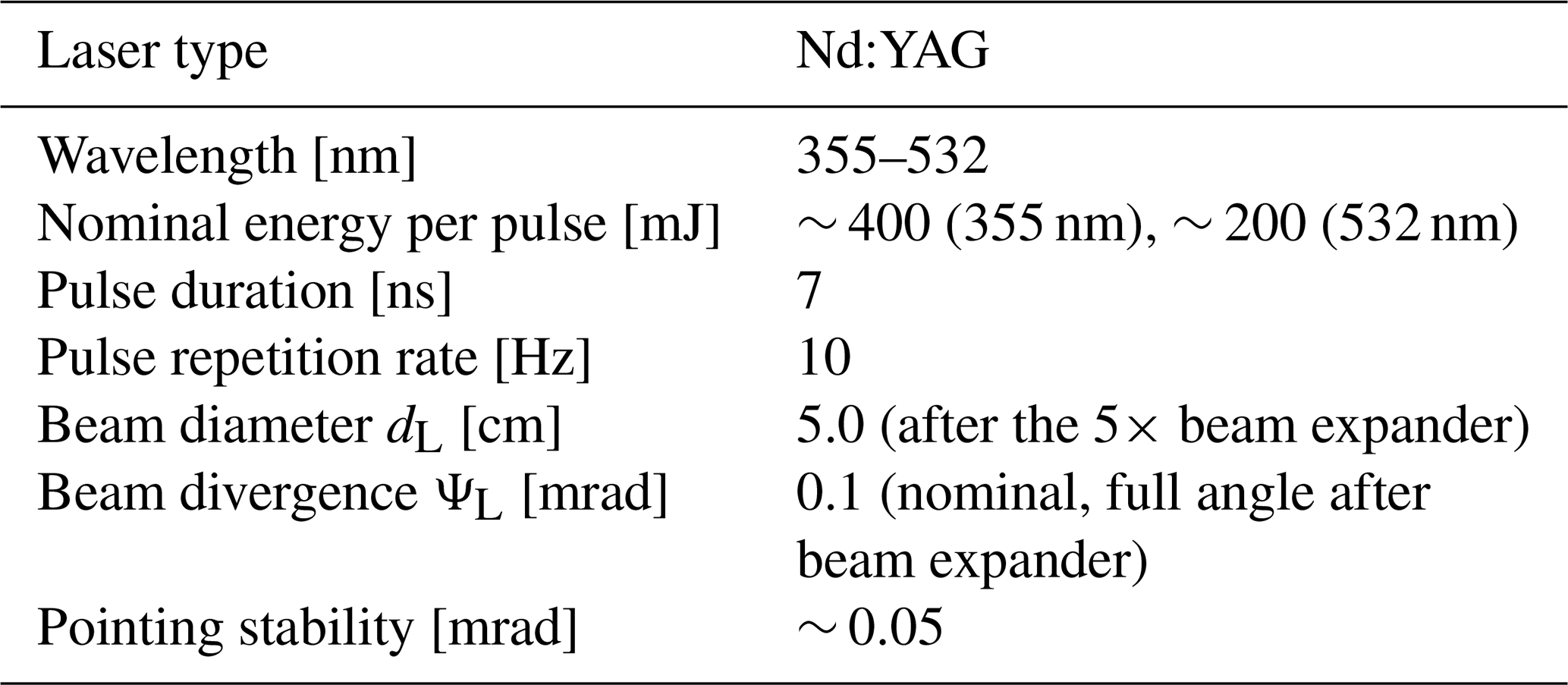
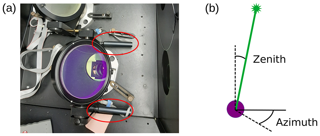
Figure 1(a) Top view of the two 45∘ mirrors with azimuth and zenith servomotors (components circled in red). (b) Schematic of the mirror/beam movements.
The receiver is based on a multiple-telescope configuration allowing the sounding of a wide altitude atmospheric interval:
-
one single 15 cm aperture telescope for the lower layers,
-
one single 30 cm telescope for the middle layers,
-
an array of 9×50 cm telescopes for the upper layers (∼ 1.7 m2 total collecting area, see Fig. 2).
The characteristics of the telescopes are reported in Table 2. For each of the 11 telescopes, behind the field stop diaphragm (0.2, 0.4, 0.6, 0.8 mm diameter for the 30 cm telescope, fixed 0.8 mm for the others) that is in the focal position, there is a dichroic beam-splitting optical system that separates the signals at λ<440 nm from the ones at λ>440 nm and directs them in two different large-core optical fibres, with 0.94 mm core diameter and 0.22 numerical aperture. In this optical system (see Fig. 3 for a detailed description), a one-to-one coupling of the field diaphragm on the optical fibre is obtained employing a set of lenses (f=20 mm): first to collimate the radiation on the dichroic mirror and then to focus the resulting different wavelength signals on the input face of the respective fibre. Each receiving block has been aligned on an optical bench before being mounted on the lidar system.
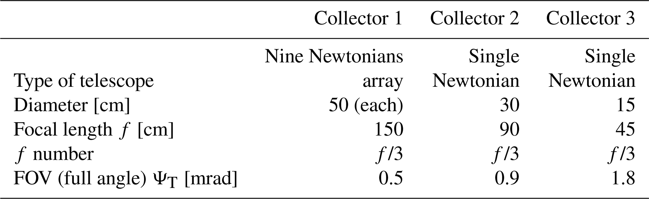

Figure 2(a) Top view schematic of the relative position of the laser beams (355 and 532) and the 11 telescopes. (b) Details of the emission and low-range telescopes (15 and 30 cm).
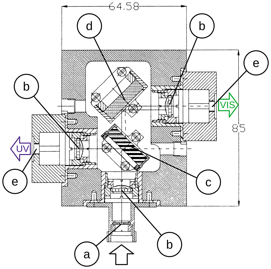
Figure 3Schematic of the receiving block: (a) field stop diaphragm (0.8 mm diameter), (b) collimation lenses (f=20 mm), (c) dichroic beam splitter (λ=440 nm), (d) 45∘ mirror, and (e) optical fibre connector. Dichroic beam splitter and UV collimation lens are currently not present in the receiving block of the 15 cm telescope.
Field diaphragm, dichroic beam-splitting optical system, and SubMiniature version A (SMA) connectors for the two optical fibre input faces are assembled in a small box supplied with adjustments for lens focusing and dichroic mirror alignment. A system of three orthogonal linear stages allows moving each box along the x, y, and z axes by means of computer-controlled servomotors, to find optimal alignment and focusing positions autonomously for each telescope.
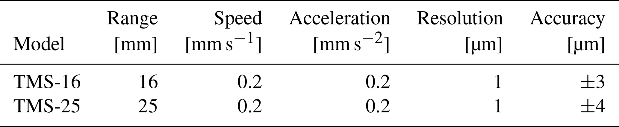
A total of 37 servomotors (three for each telescope and two for each emitting wavelength) are present. Two models of EOTECH Testine Micrometriche Servocontrollate (TMS) are used: the TMS-25 for the movements in the z-axis direction of the receiving system in the telescopes and the TMS-16 for all other movements. Table 3 reports the nominal characteristics of the employed servomotors. Each motor is controlled by a dedicated board. The boards can be connected in a serial way to control more boards with a single RS-232 serial port. A set of three racks containing up to 14 boards is used to control the motors through three serial ports. Motors belonging to a given telescope or emitting mirror are grouped in a single rack: for this reason, it is possible to control only one motor at once.
Two large carbon-fibre planes are utilized to support, respectively, the telescopes (the lower ones) and the spiders holding the x–y–z motor-moved stages with the dichroic boxes; fibreglass columns stick the two planes together. With this architecture of the telescope-supporting frame, effects on the alignment of thermal deformations are minimized. The receiving optical system with the servomotors is depicted in Fig. 4.
In the current setting, for the smallest telescope (15 cm), only the optical fibre carrying the signal return at λ>440 nm exits the dichroic system, as this telescope is used only for the elastic backscattering at 532 nm. Then, the optical fibres bring the light from the telescopes to the photomultipliers (PMTs) after passing collimating lens and interference filters that select the wavelengths of interests.
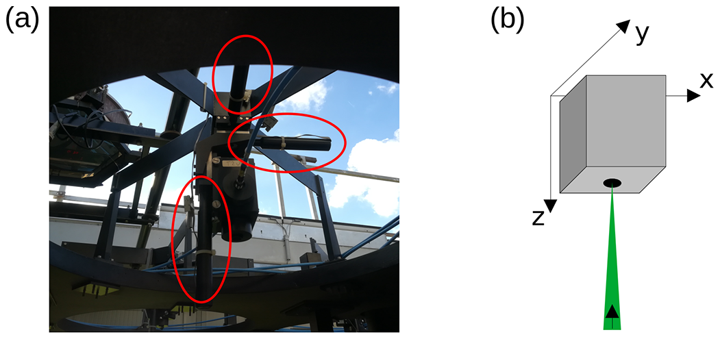
Figure 4(a) Receiving optical system with the three axis servomotors (red circled components). (b) Schematic of the receiving block movements.
Currently eight acquisition channels both in photon-counting mode as well as analogue mode are implemented; Table 4 provides an overview of the RMR channels with their associated telescopes and receiving wavelengths.
For standard measurement sessions the acquisition system is set to acquire the photon-counting mode signals for 2000 bins with a 0.5 µs integration per bin. Samples in the analogue channels are acquired at a fastest rate, with 0.05 µs sampling rate, but they are averaged in groups of 10 to have identical vertical resolution as in the counting channels and, simultaneously, to improve the accuracy of the recorded data. Thus, in the usual operation, the vertical resolution is 75 m (corresponding to 0.5 µs bins) and the signals are generally integrated over 60 s (600 laser pulses) before recording.
Table 4Wavelengths and telescopes used for each currently implemented channel.

The relative emitter–receiver geometry can be modelled knowing the characteristics of emitters and receivers (Tables 1 and 2) and the distance between the centres of each combination of emitter and receiver.
Summarizing, given
-
dcc, the distance between the centres of the laser beam and the telescope,
-
ΨL and ΨT, the divergence (full opening angle) of the laser beam and the telescope, respectively,
-
dL and dT, the beam and telescope diameter, respectively,
and assuming
-
parallel vertical axes (beam and telescope FOV),
-
aperture in the focal plane (focus at infinity),
it is possible to calculate the following geometrical characteristics relevant for the description of the overlap function O(R) (Stelmaszczyk et al., 2005):
where R0 is the lowermost height at which the laser beam enters the telescope field of view and R1 is the full overlap height (i.e. the lowermost height with O(R)=1). As an example, Fig. 5 shows the case of the 15 cm telescope and 532 nm beam. These equations are equivalent to the ones calculated from the diaphragm point of view (Halldórsson and Langerholc, 1978; Measures, 1984) taking into account the previously stated assumptions.
Table 5 completes the description of the geometry by reporting, for each telescope, the telescope diameter (dT), the field of view (ΨT), and the distance from each emitting source (dcc 532, dcc 355). Based on the nominal characteristics of the RMR system and the analytical model described above (Eqs. 1 and 2), the values of R0 and R1 have been computed for all implemented combinations of emission laser wavelengths (355 and 532 nm) and telescopes. Results are reported in Table 5. It has to be noted that the full overlap height can be optimized by tilting properly the laser beam with respect to the telescope axis (Kokkalis, 2017).
Table 5Characteristics, initial (R0) and full (R1) overlap heights of the 11 telescopes for each emitted wavelength. Laser beam radius dL=5.0 cm and divergence ΨL=0.1 mrad were used for the calculations. The specifications of interest for this study (channel 1: 532 nm, 15 cm telescope) are highlighted in bold. NA = not available.

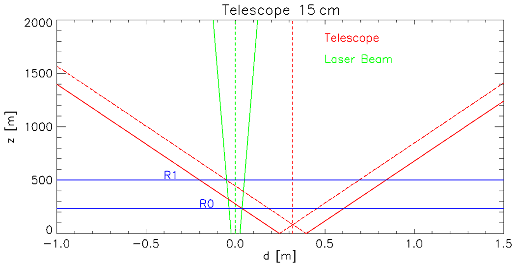
Figure 5Schematic of the overlap between the telescope FOV (red) and the laser beam (green). Full overlap is reached inside the cone delimited by the dash–dotted lines. R0 and R1 heights are highlighted by the horizontal lines.
A more realistic theoretical estimation of the whole overlap function is possible. However, it requires accurate knowledge of the real characteristics and positions of the optical parts of the system (e.g. beam shape, relative inclination between the laser beam and telescope axis). The estimation of these parameters needs a characterization of the lidar emitting–receiving components that is often difficult to perform. The proposed approach to characterize the geometry of the signal (Sect. 3) allows an estimation of the overlap function (Sect. 4.2).
The following sections will focus on the characterization of channel 1 (532 nm, 15 cm telescope). This is the channel dedicated to the PBL sensing, for which the knowledge of the overlap function is fundamental. The procedure described is however applicable to all the remaining laser/telescope combinations for quality control and signal optimization.
The mapping procedure takes advantage of the possibility of investigating the dependency of the acquired signal S(R) from the relative transmitter–receiver geometry by controlling the orientation of the laser beam and the 3D position of the diaphragm of the receiving optical system around the focal point of the telescopes. The procedure is based on a set of programs controlling both the signal acquisition as well as the motor movements, and it is fully defined by setting the following variables:
-
telescope/laser beam of interest
-
reference/starting position (x0, y0, z0 for the telescopes, Az0, Zen0 for the laser beams);
-
range and regular step in each direction independently (i.e. number of acquisitions);
-
channels to be acquired;
-
acquisition characteristics (e.g. duration, bin size).
Defining these parameters is a trade-off between having detailed and low-noise information and minimizing the signal variability introduced by changes in the atmosphere and in the lidar system (e.g. laser power). To minimize the atmospheric variability, the mapping procedure should be preferably performed in stable meteorological conditions (e.g. end of the night). However, strategies to monitor/account for these variabilities have been implemented and will be discussed for each example of mapping reported.
The single telescope and laser mapping are described in detail in the following subsections.
3.1 Telescope mapping
The telescope mapping procedure controls the position of the optical system in all three axes. This procedure is implemented by performing, for a given set of z positions, a series of acquisitions in the horizontal plane (x and y directions). Each x–y plane is scanned starting from a reference position (x0, y0) along a spiral path, in order to minimize the necessary motor movements (see example in Fig. 6).
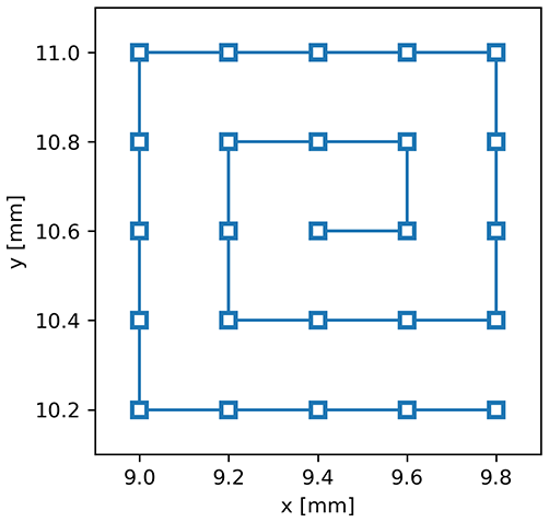
Figure 6Example of telescope mapping geometry in the x–y plane (used for the first measurement session described in this work); x and y relative position of the servomotors in the respective axis.
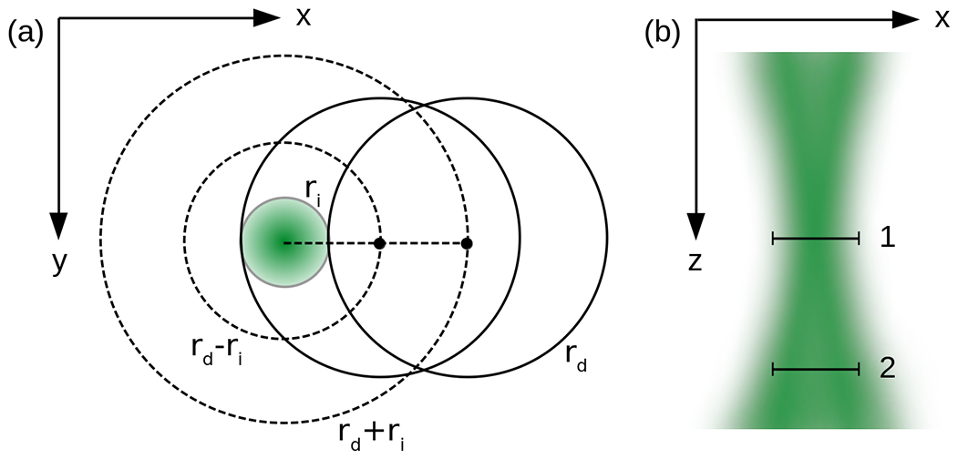
Figure 7(a) Expected radii for maximum (rd−ri) and partial counts (rd+ri) in the signal map for an image of radius ri and a diaphragm (solid line) of radius rd for ri<rd. (b) Schematic longitudinal view of radiation intensity near the focal plane, diaphragm in a focused (1) and in an out-of-focus (2) position.
Given the relative dimension of the diaphragm and the optical fibre core and assuming a well-aligned receiving box, the procedure presented in this study takes into account only the characterizable effect of the field stop diaphragm displacement.
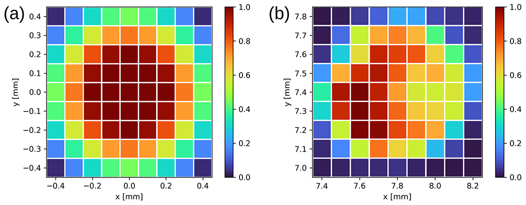
Figure 8(a) Simulated signal map for a diaphragm of radius rd=0.4 mm and an image of radius ri=0.2 mm. The signal is normalized by the maximum value. (b) Result of a single-plane mapping performed with misaligned optics; here the signal (normalized by the maximum value) is asymmetrically clipped by the optical system between the telescope and the photomultiplier.
Moving the diaphragm in the x–y plane on a fixed z for an image of radius ri<rd, where rd is the diaphragm radius, approximately constant counts are expected in a circle of radius rd−ri and a decrease to zero counts within a radius rd+ri (Fig. 7a). This of course under the assumption that all the signal passing through the diaphragm is captured by the PMT. When the signal is clipped in the path between the aperture and the sensor, the obtained mapping could be asymmetric and could diverge from the expected shape. The resulting image could also be affected by inhomogeneities in the PMT sensitivity (Freudenthaler, 2004); the use of optical fibres effectively acts as a light scrambler minimizing the impact of this problem (Sherlock et al., 1999). Small imperfections in the beam cross section, when the image is small and well-focused, should not cause asymmetries in the resulting mapping.
For a fixed range R in lidar-acquired profiles, when changing the z coordinate of the field stop/diaphragm, the image is expected to grow from the minimum in the focused position following the enlargement of the circle of confusion. If the image size is bigger than the receiving optical component (e.g. diaphragm, optical fibre, lens), part of the signal will be lost but the mapping will still be symmetric (Fig. 7b).
From the qualitative analyses of acquired signals from a single telescope mapping, knowing the ideal behaviour, it is possible to diagnose deviations from the nominal positions for all the optical components in the system not taken into account by the simplified model. As an example, Fig. 8 depicts a simulated single-plane mapping in case of good alignment and a real mapping showing problems with the optical alignment (i.e. signal clipping in the optical system between the telescope and the photomultiplier).
The information given by this type of mapping can be used to accurately position the receiving optical system as shown in Sect. 4. Another potential use of the information derived from the mapping is to estimate unknown characteristics of the system.
As an example, the relative tilt between the field of view axis and the laser beam can be computed once the centre of the image in the focal plane (xc, yc) is found. For high ranges, this position corresponds to a configuration with parallel beam and field of view axes. If the measurements are done at different positions of the receiving system in the horizontal plane, the relative tilt angle θtilt can be calculated for any given position (x, y) with the following formula:
where f is the telescope focal length and D is the geometric distance between the position x, y and the reference position xc, yc.
As previously mentioned, a trade-off between obtaining a reasonable signal-to-noise ratio (SNR) in the range of interest and minimizing possible changes in the signals due to atmospheric and system variability is needed.
In order to account for atmospheric/system variability, two approaches have been tested:
-
If there is a channel acquiring information at the same wavelength of the channel being mapped but through another telescope, a normalized signal is obtained from the ratio of the profiles from the two channels. For example, the normalized signal used for the mapping of channel 1 described in the following section (Sect. 4.1) is defined as the ratio of the simultaneously acquired measurements from channel 1 and 2 (Table 4).
-
In the absence of a suitable signal from a second channel, the signal profile from the same channel, acquired periodically in a reference position (e.g. the position chosen with a previous alignment) during the mapping, can be used to normalize the measurements within the interval of time between acquisitions in the reference position. This approach is used in the laser mapping (Sects. 3.2 and 4.2); in this case the normalized signal was calculated as .
3.2 Laser mapping
In the case of lidar systems with the capability of electronically controlled azimuth and zenith orientation of the laser beam, an analogous procedure can be implemented, leading to similar insights into the geometry of the system.
For a given telescope-laser relative geometry the overlap function can be estimated through a mapping performed varying the laser beam zenith and azimuth angle. The lowermost range for which the overlap function can be estimated depends on the characteristics of the system being required that the laser beam can be tilted to have some position with full overlap. Moreover, in order to define an absolute maximum with O(R)=1, the size of the image has to be smaller than the diaphragm (i.e. the image is sufficiently focused).
The scan is performed progressively, minimizing the necessary motor movements (Fig. 9) and the subsequent delay between acquisitions. To monitor changes in the atmospheric conditions and in the power output of the laser, an acquisition in a reference laser position (e.g. the setup chosen with the telescope mapping and used for routine measurements) is performed before and after each zenith swipe. This is highlighted in Fig. 9, where at the beginning and at the end of each column (i.e. zenith angle swipe) the laser beam returns to the same pair of zenith and azimuth values. Time-interpolated data acquired in the reference position are used to normalize the measurements during the mapping.
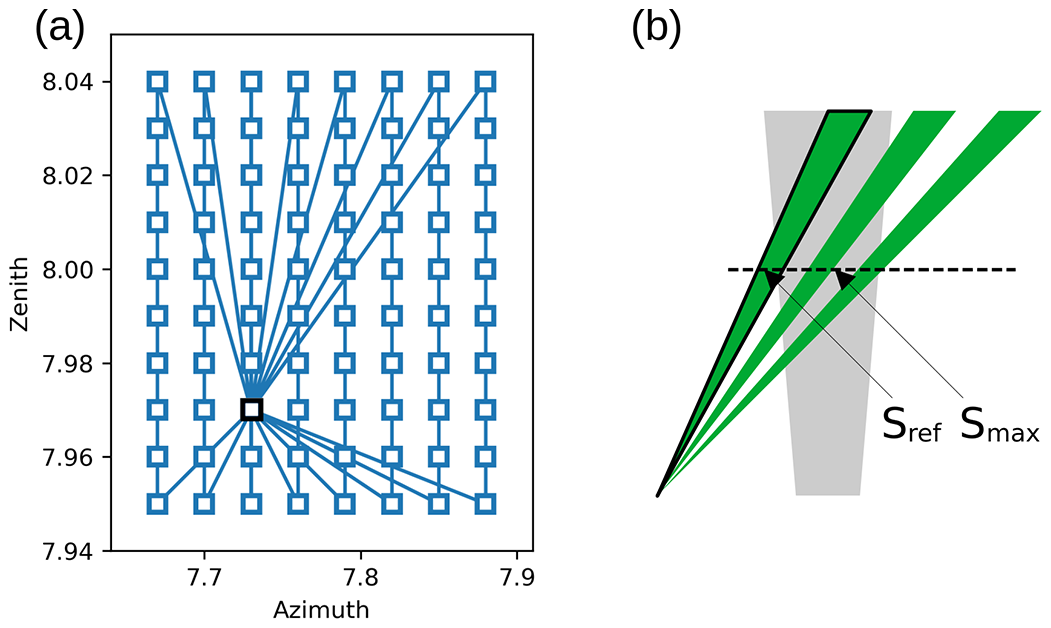
Figure 9(a) Laser mapping scan geometry, after each zenith scan a measurement in the reference position (black square) is performed. (b) Schematic of the telescope FOV and laser beam for different orientations.
To estimate the overlap function, for each range value R, the maximum (or the mean of the highest n values if the mapping is performed with sufficient x–y resolution) of the normalized signal is sought. Under the previously stated assumptions, this value should represent the ratio of a full overlap signal and affected by partial overlap. Consequently, for a given range R, the overlap factor in the reference position is . We therefore calculate the overlap function O(R) for each R between the minimum range with useful signal and the range in which the full overlap is reached.
4.1 Telescope mapping and alignment
The objective of this telescope mapping session is to optimize the alignment relative to the acquisition of 532 nm elastic backscatter by the 15 cm telescope (CH01). This has been performed in two steps:
-
a preliminary mapping with a larger range and a coarser step in the three dimensions to identify the sub-volume of optimal alignment;
-
a mapping in the sub-volume identified in the first mapping, close to the optimal position and with finer resolution.
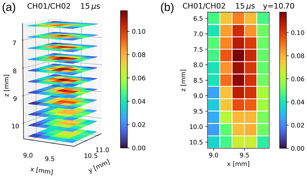
Figure 10Overall view (a) and x–z section (b) of the results of the telescope mapping of the first session (13 January 2021) showing the normalized signal as a function of the x–y–z positions at a chosen range (15 µs – 2250 m a.g.l.).
Two steps are needed due to the time necessary to perform a scan with both large x–y–z range and step. The first mapping could be skipped if the system was recently aligned.
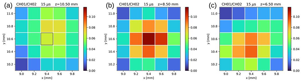
Figure 11Signal mapping of the first session (13 January 2021) showing the normalized signal for three planes at different z positions and chosen range (15 µs – 2250 m a.g.l.). The position derived from the manual alignment is highlighted by the black square.
The two sessions were performed on 13 January 2021 (18:01–23:04 UTC) and on 26 January 2021 (17:02–20:01 UTC).
Table 6 reports the characteristics of the performed mapping.
Table 6Characteristics of the two telescope mapping sessions and the laser mapping session; the channels used for the procedure are highlighted in bold.
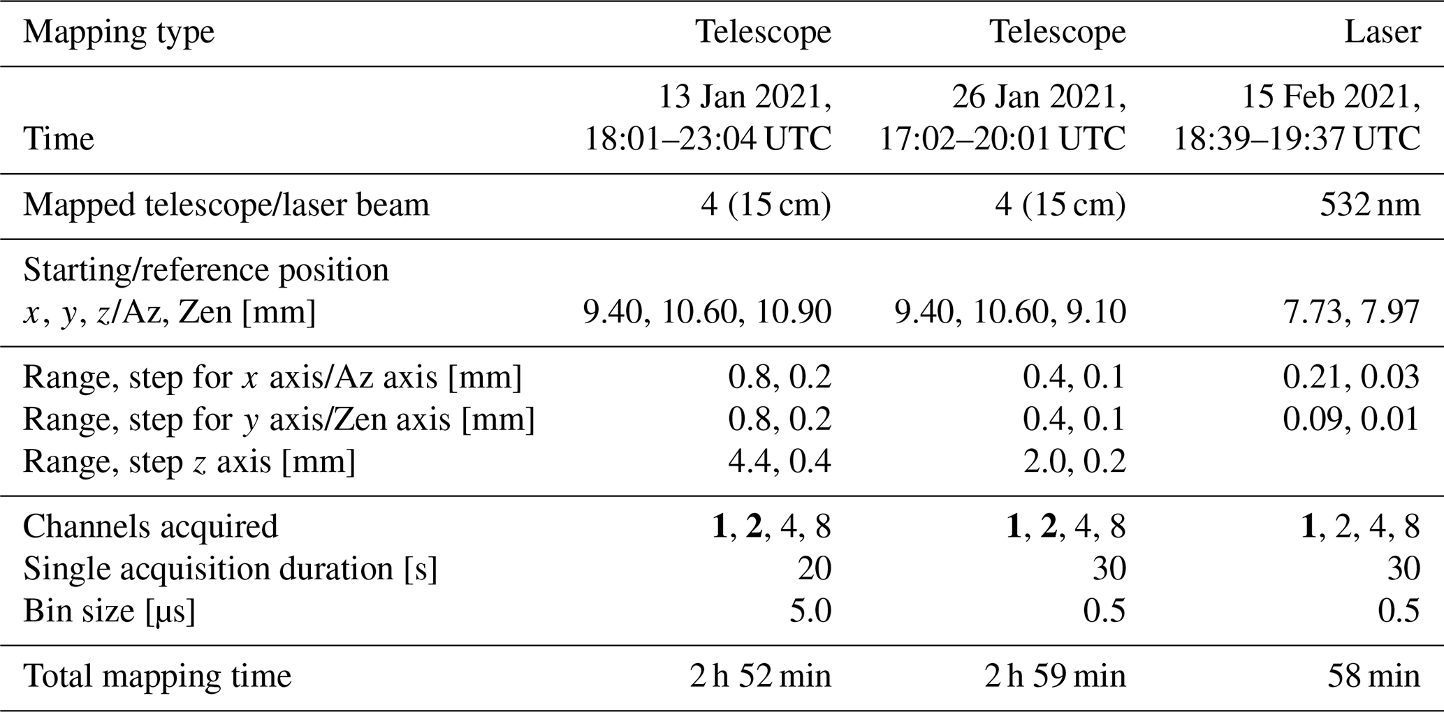
With these settings, each acquisition for the mapping procedure took about 38 s of which 30 s are the effective acquisition time and 8 s are dedicated to the data transfer and the movement of the motors that can be performed one motor at a time.
From the results, which are depicted in Figs. 10 and 11, it is clear that the telescope in the manually optimized configuration (x=9.40 mm, y=10.50 mm, z=10.50 mm, highlighted in Fig. 11a), despite being not far from the optimal x–y position, is highly out of focus due to its z position. The overall intensity of the signal in the x–y plane increases, changing the z position (Fig. 11b), as the now focused image passes through the diaphragm without being clipped. Moving further in the z axis, the signal starts again to decrease (Fig. 11c). No clear asymmetries in the signal are found. The presumed optimal position resulting from this session is x=9.40 mm, y=10.60 mm, z=8.50 mm.
The slight shift of the image centre (i.e. the centre of the area with maximum values) at different z positions is caused by incoming light rays tilted with respect to the z axis. Moreover, looking at the uppermost useful range, for x–y positions at the centre of the image the beam and telescope axis (more precisely the FOV axis) should be approximately parallel. Assuming the z axis as vertical, this information can be used to estimate the tilt of the laser beam dividing the x–y shift of the centre of the image by the z displacement, resulting in a tilt of ∼ 50 mrad.

Figure 12Signal mapping (CH01 photon-counting signal) of the second session (26 January 2021) at same z and different ranges (a: 5.0 µs – 750 m; b: 10.0 µs – 1500 m; c: 20.0 µs – 3000 m). Here the signal is not normalized due to the lack of sufficient SNR from the second channel in the lower range (highly incomplete overlap).
The second session was performed with finer steps and centred around the presumed optimal position. In Fig. 12 is plotted the signal intensity S at different ranges and a fixed z coordinate. In this case, the signal has not been normalized due to highly incomplete overlap of the second channel in the low range. The atmospheric and power variability has been monitored qualitatively with channel-2 measurements at higher ranges. In the x–y plane, as expected, the image shifts at different altitudes. No evident asymmetries are present in the signal map.
Through this session, a definitive and well-aligned position can be selected in the x–y plane as a trade-off between maximizing counts in the lower range (optimizing the signal in the partial overlap range and lowering the full overlap height) and maintaining the beam in the telescope FOV at high ranges.
In the z coordinate, the optimal position is selected evaluating the normalized signals at a medium range around the selected x and y position. As shown in Fig. 13, the curve has a plateau in which the maximum value is reached (i.e. the image is sufficiently focused and inside the diaphragm). The selection of a position in the higher-value portion of the plateau corresponds to a diaphragm position that better captures the signal in the lowermost range (the focus shifts from infinity to lower ranges).
Based on the above considerations the derived optimal position is x=9.45 mm, y=10.55 mm, z=8.30 mm.
As mentioned in Sect. 3.1, measuring the angular distance between the selected position and the centre of the image at high ranges (Eq. 3), the relative tilt between the telescope FOV axis and the laser beam is about 0.3 mrad.
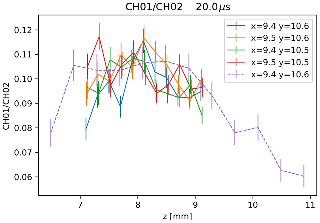
Figure 13Normalized signal at a chosen range (20 µs – 3000 m) for different x and y positions as a function of z; data from both mapping sessions (dashed line for the first session, solid line for the second). A plateau is reached approximately between z=7 mm and z=9 mm. Each colour corresponds to different x and y positions as indicated in the legend of the plot.
4.2 Alignment validation
The selected alignment configuration was validated through a telecover test and direct comparison of the signal profiles in the different positions.
The telecover test, described by Freudenthaler et al. (2018), is a quality assurance tool used for lidar system misalignment diagnostic and evaluation of the full overlap range. Lidar profiles taken with different sectors of the telescope aperture are compared to each other. For well-designed and correctly aligned systems, the normalized signals should only show differences in the partial overlap range.
Measurements were carried out during a single night session (2 February 2021, 18:55–21:26 UTC). Progressively the following measurements were performed (see Fig. 14): a telecover test in the non-optimized starting position (a), a full telescope measurement in the same position (b) and one in the optimized position (c), and finally a telecover test in the optimized position (d). Standard acquisition times were used (60 s), with an integration time of 10 min for each telecover test sector or comparison profile.
4.2.1 Profile comparison
Figure 15a shows the direct comparison of the background subtracted signal profiles in the non-optimized starting position and in the optimized position. Higher signal is found in the whole optimized profile (>50 % relative normalized difference), confirming the successful alignment procedure and no signal loss in the high range (Fig. 15b). The negative difference in the lowermost range is well below the full overlap height (i.e. <500 m) and can be explained considering that the large and less focused image of the non-optimized position can maintain a partial overlap with the telescope FOV for a wider vertical range.
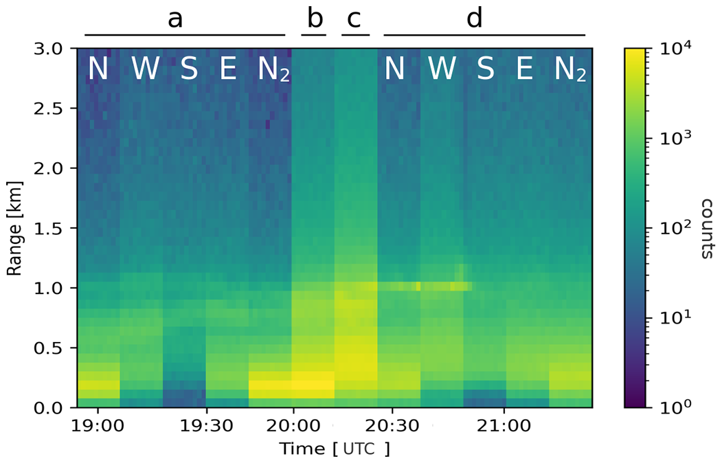
Figure 14Validation measurement session (2 February 2021). Telecover (a) and full telescope measurement in the non-optimized position (b) and in the optimized position (d and c, respectively).

Figure 15Background subtracted counts (a) and relative difference between the normalized signal profiles (b) in the selected position (x=9.45 mm y=10.55 mm z=8.30 mm) and the starting one (x=9.40 mm y=10.50 mm z=10.50 mm).
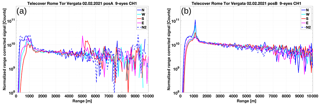
Figure 16Telecover test results for the positions selected with manual (a) and mapping-based (b) alignment procedures.
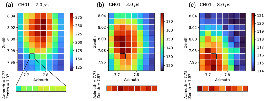
Figure 17Laser mapping signal (CH01 analogue signal before normalization with the reference position signal) at three different ranges expressed as delays at the top of the bin (a: 2.0 µs – 300 m; b: 3.0 µs – 450 m; c: 8.0 µs – 1200 m). The reference position (Az = 7.73, Zen =7.97) is highlighted by the black square. Measurements in this position are acquired every zenith acquisition sequence and are represented in the lower array.
4.2.2 Telecover
Two telecover tests were conducted: one in the non-optimized starting position (Fig. 16a) and one in the optimized position (Fig. 16b). Figure 16a shows that the height of full overlap is higher than 1500 m, far from the expected modelled value of 501 m (see Table 5). Assuming a negligible impact of mirror imperfections and the irregular shape of the laser beam, this has been confirmed to be due to the diaphragm in an out-of-focus position for the z axis. This leads to an image in the aperture plane with a large circle of confusion and non-optimal alignment of the field of view (x and y axes).
Figure 16b depicts the results in the optimized position. The full overlap height is around 1000 m or less, and the relative difference of the signals in the partial overlap region has decreased. Atmospheric variability and the presence of aerosol layers prevent a more precise evaluation of the overlap height using the telecover QA method. As expected, less noise is detected in all ranges due to the increased signal.
4.3 Laser mapping and overlap estimation
Once an optimized position has been selected and verified (see Sect. 4.1 and 4.2), a laser beam mapping with the purpose of estimating the overlap function was performed (15 February 2021, 18:39–19:37 UTC). The characteristics of the mapping are reported in Table 6. In Fig. 17 the mapped analogue signal at three different ranges is shown. As in the telescope mapping, a range-dependent shift of the signal away from the reference position is visible in the lowermost range.
From this data, the overlap function using the methodology presented in Sect. 3.2 is calculated. The first five highest values are used for the calculation of at each range. In order to evaluate the possible impact of the dead-time effect in the PC mode (Donovan et al., 1993; Cairo et al., 1996), the analysis was performed also using data acquired in the analogue mode. Figure 18 shows the estimated overlap function from analogue (A) and photon-counting (PC) data; the resulting uncertainty is evaluated by the propagation of the signal uncertainties. As a reference, Fig. 18 also shows the overlap function computed with an analytical model with uniform beam energy distribution (Stelmaszczyk et al., 2005) and a Monte Carlo integration of Halldórsson and Langerholc (1978) equations with Gaussian beam energy distribution. Both models use the relative inclination of the laser beam estimated via the telescope mapping (see Sect. 4.1).

Figure 18Estimated overlap function using analogue (A) and photon-counting (PC) data compared to the overlap function calculated from models with the assumption of a uniform/Gaussian beam, diaphragm in the focal plane, and tilted beam (0.3 mrad).
The function O(R) reaches unity in the expected range and the experimental results are in agreement with the models. Photon-counting data were corrected for trigger delays (Freudenthaler et al., 2018) as described in Appendix A. One evident feature is that after having reached the maximum (at 500–800 m) the values start to slowly decrease. This underestimation of the retrieved overlap function in the high ranges can be explained by the methodology chosen for the maxima selection. In particular, the systematic overestimation of the maxima (due to the shot noise) becomes relevant only above the range of interest (i.e. where O(R) has already reached unity). The difference between the modelled/retrieved full overlap height and the one found via the telecover test could be due to aerosol variability in the latter or slight instabilities of the system beam/telescope alignment and needs to be further investigated.
As an example of the application, Fig. 19 shows an uncorrected aerosol backscattering profile and the corrected one using the PC-retrieved overlap function applied from 200 to 500 m for channel 1 (11 February 2021, 19:45–20:44 UTC). Both the uncertainty associated with the overlap for the first four bins and the retrieval algorithm uncertainty have been taken into account for the corrected profile. Applying the overlap correction allows the extension of the useful range of the aerosol backscattering profile down to 200 m.
Taking advantage of the capability of the RMR 9-eyes lidar system to electronically control, with motors, the orientation of the laser beam and the position of the receiving optical system around the focal point of the telescopes, a mapping procedure was developed to characterize the dependency of the acquired signal from the system relative transmitter–receiver geometry. The procedure consists in a set of programs controlling both the signal acquisition as well as the motor movements. The developed approach also includes solutions to account for atmospheric and laser power variability likely to occur during the mapping sessions. The mapping procedure allows applications such as the optimization of the telescope/beam alignment and the estimation of the overlap function. It should be noted that the results of the procedure can also be used to diagnose the overall optical alignment and verify the adopted assumptions.
To optimize the RMR system for the objectives of ACTRIS/EARLINET (e.g. the description of aerosol optical properties in the lower troposphere and PBL), this procedure was applied to the single combination of telescope and laser beam (15 cm telescope, 532 nm) of the system that senses this region of the atmosphere better.
Another output of the procedure was the estimation of the absolute tilt of the laser beam with respect to the z axis (∼ 50 mrad) and the relative tilt with respect to the FOV axis (∼ 0.3 mrad). Such values are fundamental to model the dependency of the signal from the system geometry.
The presented methodology was tested to obtain an optimized laser-telescope configuration starting from a non-optimized one. The mapping procedure diagnosed an out-of-focus image and identified the correct z position. As a result, the signal intensity increased in the whole channel 1 profile with respect to the previous configuration. The effectiveness of the procedure was verified comparing the results of a telecover test before and after the alignment. The new configuration resulted in a lower full overlap height (from 1500 m to less than 1000 m).
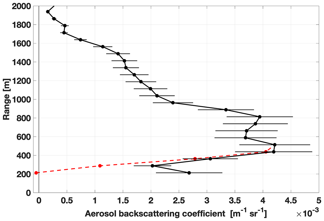
Figure 19Aerosol backscattering coefficient (11 February 2021, 19:45–20:44 UTC); comparison between the overlap-corrected (solid black line) and uncorrected (dashed red line) profile.
Once an optimized position has been selected and verified, a laser beam mapping with the purpose of estimating the overlap function was performed. The retrieved function was compared to the ones modelled using as input the parameters obtained from the procedure showing good agreement. Correcting the lidar profiles of channel 1 with this function allows extending the useful range down to 200 m.
The developed mapping procedure will be applied to the remaining channels in order to characterize each transmitter–receiver combination. Based on the retrieved information it will be possible to define a set of configurations aimed to satisfy the different scientific objectives (e.g. PBL, upper troposphere–lower stratosphere). A simplified mapping procedure can be used to complement the standard EARLINET quality assurance tests. For example, a protocol coupling telecover test and mapping session are currently implemented in the RMR system. Monthly mappings are performed to monitor and optimize the alignment and to estimate the overlap function, whereas periodically required telecover tests (e.g. 1–2 times per year) check and attest the obtained alignment and identify the minimum height with full overlap.
Besides the applications presented in this study, a similar approach could be adapted also to lidar systems with different hardware capabilities to provide essential information about their transmitter–receiver geometry that is needed for a complete characterization of the received signal.
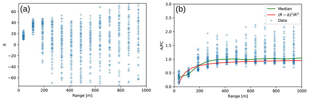
The lidar photon-counting data range was corrected for trigger delay relatively to the analogue data range using the following procedure. Assuming a linear relation between photon-counting and analogue data (i.e. no saturation) and after correcting the latter for voltage offset and dividing it by the proportionality constant between the two, it is possible to write the following equations:
where A is the corrected analogue signal, PC is the photon-counting signal, f(R) is a function encompassing all the lidar equation terms apart from the inverse square law, and Δ is the spatial delay between analogue and photon-counting sampling ranges.
For low R a limited dependence of the function f on R variations with respect to the inverse square law can be assumed. This is true especially for the first bins where limited or no overlap is present and most of the signal comes from laser secondary reflections and multiple scattering:
Under this assumption, the ratio of the analogue and photocounting signals is
from which it is possible to derive the difference Δ as a function of R:
Figure A1a depicts the retrieved spatial delay computed with Eq. (A5) using laser mapping data from Sect. 4.3. The assumptions hold for the first two bins from which a delay of ∼ 25 m can be derived using an average value. For higher ranges, the overlap function dependency from R begins to be relevant, preventing the computation of the delay (i.e. the assumption in Eq. (A3) is not valid anymore). This dependency is not definite and partially randomized due to the variable emitting geometry and resulting overlap function of the mapping lidar profiles. Once a delay is retrieved the ratio can be plotted and compared with the range function ( (Fig. A1b). As shown in Fig. A1b, the computed range function represents the normalized ratio well.
Code and data are available upon request by contacting the authors.
MDP, GLL, and DD conceived the concept of this study. MDP, GLL, and DD performed the lidar measurements. MDP developed the presented methods, processed the data, and carried out the analysis. MDP, GLL, and DD contributed to the interpretation, the validation, and the visualization of the results. MDP wrote the original draft with input from all other co-authors. All co-authors provided the review and the editing of the paper.
The contact author has declared that neither they nor their co-author has any competing interests.
Publisher’s note: Copernicus Publications remains neutral with regard to jurisdictional claims in published maps and institutional affiliations.
We acknowledge Sara Piermarini and Roberto Massimo Leonardi for the development of the first versions of the motor control software. We also acknowledge Raffaello Foldes for his contribution in the early development of the mapping procedure. We thank Francesco Cardillo for the help in performing lidar measurements.
This paper was edited by Simone Lolli and reviewed by two anonymous referees.
Cairo, F., Congeduti, F., Poli, M., Centurioni, S., and Di Donfrancesco, G.: A survey of the signal-induced noise in photomultiplier detection of wide dynamics luminous signals, Rev. Sci. Instrum., 67, 3274–3280, https://doi.org/10.1063/1.1147408, 1996.
Campanelli, M., Estelles, V., Smyth, T., Tomasi, C., Martìnez-Lozano, M. P., Claxton, B., Muller, P., Pappalardo, G., Pietruczuk, A., Shanklin, J., Colwell, S., Wrench, C., Lupi, A., Mazzola, M., Lanconelli, C., Vitale, V., Congeduti, F., Dionisi, D., Cardillo, F., Cacciani, M., Casasanta, G., and Nakajima, T.: Monitoring of Eyjafjallajökull volcanic aerosol by the new European Skynet Radiometers (ESR) network, Atmos. Environ., 48, 33–45, https://doi.org/10.1016/j.atmosenv.2011.09.070, 2012.
Chourdakis, G., Papayannis, A., and Porteneuve, J.: Analysis of the receiver response for a noncoaxial lidar system with fiber-optic output, Appl. Opt., 41, 2715–2723, https://doi.org/10.1364/AO.41.002715, 2002.
Comeron, A., Sicard, M., Kumar, D., and Rocadenbosch, F.: Use of a field lens for improving the overlap function of a lidar system employing an optical fiber in the receiver assembly, Appl. Opt., 50, 5538–5544, https://doi.org/10.1364/AO.50.005538, 2011.
Congeduti, F., Marenco, F., Baldetti, P., and Vincenti, E.: The multiple-mirror lidar “9-eyes,” J. Opt. Pure Appl. Opt., 1, 185–191, https://doi.org/10.1088/1464-4258/1/2/012, 1999.
D'Amico, G., Amodeo, A., Baars, H., Binietoglou, I., Freudenthaler, V., Mattis, I., Wandinger, U., and Pappalardo, G.: EARLINET Single Calculus Chain – overview on methodology and strategy, Atmos. Meas. Tech., 8, 4891–4916, https://doi.org/10.5194/amt-8-4891-2015, 2015.
D'Aulerio, P., Fierli, F., Congeduti, F., and Redaelli, G.: Analysis of water vapor LIDAR measurements during the MAP campaign: evidence of sub-structures of stratospheric intrusions, Atmos. Chem. Phys., 5, 1301–1310, https://doi.org/10.5194/acp-5-1301-2005, 2005.
Dho, S. W., Park, Y. J., and Kong, H. J.: Experimental determination of a geometric form factor in a lidar equation for an inhomogeneous atmosphere, Appl. Opt., 36, 6009–6010, https://doi.org/10.1364/AO.36.006009, 1997.
Dionisi, D., Congeduti, F., Liberti, G. L., and Cardillo, F.: Calibration of a Multichannel Water Vapor Raman Lidar through Noncollocated Operational Soundings: Optimization and Characterization of Accuracy and Variability, J. Atmos. Ocean. Technol., 27, 108–121, https://doi.org/10.1175/2009JTECHA1327.1, 2010.
Dionisi, D., Keckhut, P., Hoareau, C., Montoux, N., and Congeduti, F.: Cirrus crystal fall velocity estimates using the Match method with ground-based lidars: first investigation through a case study, Atmos. Meas. Tech., 6, 457–470, https://doi.org/10.5194/amt-6-457-2013, 2013a.
Dionisi, D., Keckhut, P., Liberti, G. L., Cardillo, F., and Congeduti, F.: Midlatitude cirrus classification at Rome Tor Vergata through a multichannel Raman–Mie–Rayleigh lidar, Atmos. Chem. Phys., 13, 11853–11868, https://doi.org/10.5194/acp-13-11853-2013, 2013b.
Dionisi, D., Barnaba, F., Diémoz, H., Di Liberto, L., and Gobbi, G. P.: A multiwavelength numerical model in support of quantitative retrievals of aerosol properties from automated lidar ceilometers and test applications for AOT and PM10 estimation, Atmos. Meas. Tech., 11, 6013–6042, https://doi.org/10.5194/amt-11-6013-2018, 2018.
Donovan, D. P., Whiteway, J. A., and Carswell, A. I.: Correction for nonlinear photon-counting effects in lidar systems, Appl. Opt., 32, 6742–6753, https://doi.org/10.1364/AO.32.006742, 1993.
Freudenthaler, V.: Effects of Spatially Inhomogeneous Photomultiplier Sensitivity on LIDAR Signals and Remedies, Eur. Space Agency Spec. Publ. ESA SP, 561, 37, 2004.
Freudenthaler, V., Linné, H., Chaikovski, A., Rabus, D., and Groß, S.: EARLINET lidar quality assurance tools, Atmos. Meas. Tech. Discuss. [preprint], https://doi.org/10.5194/amt-2017-395, in review, 2018.
Guerrero-Rascado, J. L., Costa, M. J., Bortoli, D., Silva, A. M., Lyamani, H., and Alados-Arboledas, L.: Infrared lidar overlap function: an experimental determination, Opt. Express, 18, 20350–20369, https://doi.org/10.1364/OE.18.020350, 2010.
Halldórsson, T. and Langerholc, J.: Geometrical form factors for the lidar function, Appl. Opt., 17, 240–244, https://doi.org/10.1364/AO.17.000240, 1978.
Jenness, J. R., Lysak, D. B., and Philbrick, C. R.: Design of a lidar receiver with fiber-optic output, Appl. Opt., 36, 4278–4284, https://doi.org/10.1364/AO.36.004278, 1997.
Kokkalis, P.: Using paraxial approximation to describe the optical setup of a typical EARLINET lidar system, Atmos. Meas. Tech., 10, 3103–3115, https://doi.org/10.5194/amt-10-3103-2017, 2017.
McGill, M. J., Yorks, J. E., Scott, V. S., Kupchock, A. W., and Selmer, P. A.: The Cloud-Aerosol Transport System (CATS): a technology demonstration on the International Space Station, in: Lidar Remote Sensing for Environmental Monitoring XV, Proc. Spie., 96120A, https://doi.org/10.1117/12.2190841, 2015.
Measures, R. M.: Laser remote sensing: Fundamentals and applications, John Wiley & Sons, Inc., Hoboken, 1st Edn., 510 pp., ISBN: 978-0-471-08193-7, 1984.
Pappalardo, G., Amodeo, A., Apituley, A., Comeron, A., Freudenthaler, V., Linné, H., Ansmann, A., Bösenberg, J., D'Amico, G., Mattis, I., Mona, L., Wandinger, U., Amiridis, V., Alados-Arboledas, L., Nicolae, D., and Wiegner, M.: EARLINET: towards an advanced sustainable European aerosol lidar network, Atmos. Meas. Tech., 7, 2389–2409, https://doi.org/10.5194/amt-7-2389-2014, 2014.
Sasano, Y., Shimizu, H., Takeuchi, N., and Okuda, M.: Geometrical form factor in the laser radar equation: an experimental determination, Appl. Opt., 18, 3908–3910, https://doi.org/10.1364/AO.18.003908, 1979.
Sherlock, V., Garnier, A., Hauchecorne, A., and Keckhut, P.: Implementation and validation of a Raman lidar measurement of middle and upper tropospheric water vapor, Appl. Opt., 38, 5838–5850, https://doi.org/10.1364/AO.38.005838, 1999.
Sicard, M., Rodríguez-Gómez, A., Comerón, A., and Muñoz-Porcar, C.: Calculation of the Overlap Function and Associated Error of an Elastic Lidar or a Ceilometer: Cross-Comparison with a Cooperative Overlap-Corrected System, Sensors, 20, 6312, https://doi.org/10.3390/s20216312, 2020.
Stelmaszczyk, K., Dell'Aglio, M., Chudzyński, S., Stacewicz, T., and Wöste, L.: Analytical function for lidar geometrical compression form-factor calculations, Appl. Opt., 44, 1323–1331, https://doi.org/10.1364/AO.44.001323, 2005.
Tomine, K., Hirayama, C., Michimoto, K., and Takeuchi, N.: Experimental determination of the crossover function in the laser radar equation for days with a light mist, Appl. Opt., 28, 2194–2195, https://doi.org/10.1364/AO.28.002194, 1989.
Wandinger, U. and Ansmann, A.: Experimental determination of the lidar overlap profile with Raman lidar, Appl. Opt., 41, 511–514, https://doi.org/10.1364/AO.41.000511, 2002.
Wandinger, U., Freudenthaler, V., Baars, H., Amodeo, A., Engelmann, R., Mattis, I., Groß, S., Pappalardo, G., Giunta, A., D'Amico, G., Chaikovsky, A., Osipenko, F., Slesar, A., Nicolae, D., Belegante, L., Talianu, C., Serikov, I., Linné, H., Jansen, F., Apituley, A., Wilson, K. M., de Graaf, M., Trickl, T., Giehl, H., Adam, M., Comerón, A., Muñoz-Porcar, C., Rocadenbosch, F., Sicard, M., Tomás, S., Lange, D., Kumar, D., Pujadas, M., Molero, F., Fernández, A. J., Alados-Arboledas, L., Bravo-Aranda, J. A., Navas-Guzmán, F., Guerrero-Rascado, J. L., Granados-Muñoz, M. J., Preißler, J., Wagner, F., Gausa, M., Grigorov, I., Stoyanov, D., Iarlori, M., Rizi, V., Spinelli, N., Boselli, A., Wang, X., Lo Feudo, T., Perrone, M. R., De Tomasi, F., and Burlizzi, P.: EARLINET instrument intercomparison campaigns: overview on strategy and results, Atmos. Meas. Tech., 9, 1001–1023, https://doi.org/10.5194/amt-9-1001-2016, 2016.
Weitkamp, C. (Ed.): Lidar: range-resolved optical remote sensing of the atmosphere, Springer, New York, 455 pp., 1st Edn., https://doi.org/10.1007/b106786, 2005.
Wiegner, M., Madonna, F., Binietoglou, I., Forkel, R., Gasteiger, J., Geiß, A., Pappalardo, G., Schäfer, K., and Thomas, W.: What is the benefit of ceilometers for aerosol remote sensing? An answer from EARLINET, Atmos. Meas. Tech., 7, 1979–1997, https://doi.org/10.5194/amt-7-1979-2014, 2014.
Winker, D. M., Pelon, J. R., and McCormick, M. P.: CALIPSO mission: spaceborne lidar for observation of aerosols and clouds, in: Lidar Remote Sensing for Industry and Environment Monitoring III, P. Soc. Photo.-Opt. Ins., 4893, 1–11, https://doi.org/10.1117/12.466539, 2003.