The NO₂ camera based on gas correlation spectroscopy

Spectroscopic methods have proven to be reliable and of high selectivity by utilizing the characteristic spectral absorption signature of trace gases such as NO₂. However, they typically lack the spatiotemporal resolution required for real-time imaging measurements of NO₂ emissions. We propose imaging measurements of NO₂ in the visible spectral range using a novel instrument, an NO₂ camera based on the principle of gas correlation spectroscopy (GCS). For this purpose two gas cells (cuvettes) are placed in front of two camera modules. One gas cell is empty, while the other is filled with a high concentration of the target gas. The filled gas cell operates as a non-dispersive spectral filter to the incoming light, maintaining the two-dimensional imaging capability of the sensor arrays. NO₂ images are generated on the basis of the signal ratio between the two images in the spectral window between 430 and 445 nm, where the NO₂ absorption cross section is strongly structured. The capabilities and limits of the instrument are investigated in a numerical forward model. The predictions of this model are verified in a proof-of-concept measurement, in which the column densities in specially prepared reference cells were measured with the NO₂ camera and a conventional differential optical absorption spectroscopy (DOAS) instrument. Finally, results from measurements at a large power plant, the Großkraftwerk Mannheim (GKM), are presented. NO₂ column densities of the plume emitted from a GKM chimney are quantified at a spatiotemporal resolution of $\mathrm{1}/\mathrm{12}$ frames per second (FPS) and 0.9 m×0.9 m. A detection limit of 2⋅10¹⁶ molec. cm⁻² was reached. An NO₂ mass flux of $F_{\mathrm{m}}=(\mathrm{7.4}\pm \mathrm{4.2})$ kg h⁻¹ was estimated on the basis of wind speeds obtained from consecutive images. The instrument prototype is highly portable for building costs of below EUR 2000.

1 Introduction

Oxides of nitrogen (${\mathrm{NO}}_x=\mathrm{NO}+{\mathrm{NO}}_{\mathrm{2}}$) play an important role in urban air quality. Nitrogen dioxide (NO₂) is itself toxic to humans and furthermore contributes to the formation of ozone (O₃) and particulate matter. Both NO₂ as well as ozone and particulate matter are linked to a variety of diseases, such as asthmatic and cardiovascular diseases (see, e.g., World Health Organization, 2000; Faustini et al., 2014). Recent studies have shown that in many European countries the average annual exposure to NO₂ exceeds 10 µg m⁻³ (European Environment Agency, 2017), which is the exposure limit recommended by the World Health Organization (2021). In other parts of the world exceedances are even higher. Therefore, monitoring NO₂ emissions and abundance near the planetary surface is of interest. In many cases NO₂ concentration gradients occur on small spatial (sub-meter) and temporal (sub-second) scales, e.g., when measuring the emissions of moving point sources, such as cars, ships, or airplanes. At the same time, examinations of plume geometries, mass fluxes, and chemical reactions that take place in plumes require spatial coverage of the scene. Overall, an imaging method for NO₂ with high spatiotemporal resolution could reveal more insight into the quantity and dynamics of NO₂ emissions.

In polluted regions NO_x emissions are mainly of anthropogenic origin. Combustion processes, which occur, e.g., in car motors or industrial power plants, generate NO_x, which, at the time of emission, consists mostly of NO (typically with NO₂$/$NO_x ratios as low as 5 %–10 %; see, e.g., Kenty et al., 2007, and Carslaw, 2005). Through oxidization processes, such as

$$\begin{array}{}\text{(R1)}& \mathrm{NO}+{\mathrm{O}}_{\mathrm{3}}\to {\mathrm{NO}}_{\mathrm{2}}+{\mathrm{O}}_{\mathrm{2}},\end{array}$$

or, at very high NO concentrations,

$$\begin{array}{}\text{(R2)}& \mathrm{2}\mathrm{NO}+{\mathrm{O}}_{\mathrm{2}}\to \mathrm{2}{\mathrm{NO}}_{\mathrm{2}},\end{array}$$

NO is converted to NO₂. In addition, other sources of NO_x exist, such as geophysical events like lightning strikes, forest fires or soil emissions. Due to photodissociation, i.e.,

$$\begin{array}{}\text{(R3)}& {\mathrm{NO}}_{\mathrm{2}}+h\mathit{\nu }\to \mathrm{NO}+\mathrm{O},\end{array}$$

an equilibrium between NO₂, NO, and O₃ (quickly formed by O+O₂), called the Leighton relationship, settles in.

There are different remote sensing methods for monitoring of atmospheric trace gases such as NO₂. The state-of-the-art method is differential optical absorption spectroscopy (DOAS; Platt and Stutz, 2008), in which the absorption cross sections of the target gases are fitted to the spectrally resolved differential optical depths along a light path. Then the column densities of the target gases are retrieved as fit parameters. DOAS measurements can be based on natural light sources, such as scattered sunlight, or on artificial ones. Modern DOAS spectrographs typically have a spectral resolution of <1 nm and operate in the UV and visible spectral range. The benefits of analyzing spectrally resolved data are high selectivity and low detection limits. However, grating spectrographs are less suited for imaging because spectral mapping leads to a reduced light throughput. Therefore, measurements with sufficient spatial and spectral resolution require rather long acquisition times of many minutes (Bobrowski et al., 2006; Louban et al., 2009). Imaging DOAS (I-DOAS) is typically realized using a push-broom technique, in which one detector dimension is used for spatial resolution and the other for spectral mapping. Consequently, I-DOAS requires scanning a field of view (FOV) column by column or row by row. This strategy was used, for example, by Manago et al. (2018), who report on an imaging DOAS instrument for NO₂ based on a hyperspectral camera with a spatial resolution of 640×480 pixels, a $\mathrm{13}{}^{\circ }\times \mathrm{9}{}^{\circ }$ FOV, and a frame rate of 0.2 FPS. Although modern hyperspectral cameras can reach adequate spatiotemporal resolution, some problems remain. Methods that rely on a push-broom scheme suffer from time delays between the rows (or columns) of the recorded images. Furthermore, spectrally resolving instruments are usually expensive and bulky.

We propose an imaging instrument for NO₂ based on gas correlation spectroscopy (GCS; see, e.g., Ward and Zwick, 1975, Drummond et al., 1995, Wu et al., 2018, and Baker et al., 1986) and demonstrate that an instrument designed to measure only a single trace gas can work by using reduced but specific spectral information in order to maximize spatiotemporal resolution. This is achieved by the use of two 2D photosensors, each equipped with a lens and a glass cell: one filled with air (the “empty” cell) and one filled with a high concentration of NO₂.

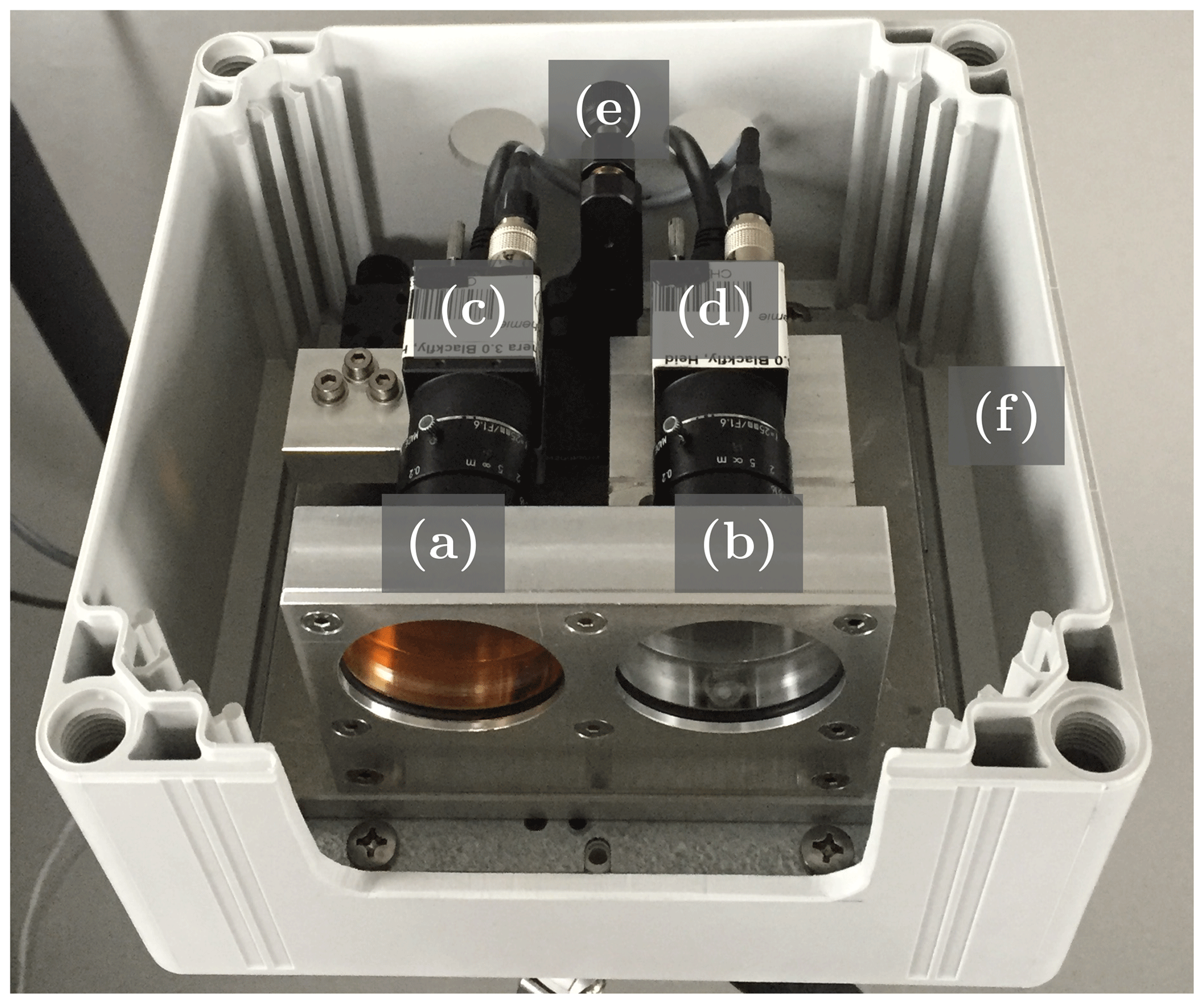
Figure 1 Photograph of the GCS-based NO₂ camera. The main parts of the instrument (see also Fig. 2a and b) are two gas cells, one filled with NO₂ (a) and one empty (b), as well as two camera modules (c, d), each with a lens and a bandpass filter. One of the camera modules is placed on a mounting stage (e), which allows for precise alignment of the optical axes. All parts are mounted into a plastic case (f).

Figure 1 shows a photograph of an instrument prototype. The NO₂ cell functions as a spectral filter to the incoming light, while the empty cell ideally has no effect on the incoming light and serves as a reference. At the same time, the cameras fully resolve the light in two spatial dimensions. This way image data with only two spectral channels (in contrast to about 100 spectral channels used for typical DOAS fitting windows) are obtained. The NO₂ column density measured by each pixel of the instrument can then be computed by application of the Lambert–Beer law to the two channels. This principle is explained in more detail in Sect. 2.1. The method is therefore similar to the recently developed filter-correlation-based SO₂ camera (Mori and Burton, 2006), the imaging Fabry–Pérot interferometer correlation spectroscopy technique (IFPICS; see, e.g., Kuhn et al., 2019, and Fuchs et al., 2021), or the acousto-optical tunable-filter-based (AOTF) NO₂ camera (Dekemper et al., 2016). However, using a gas cell has substantial advantages compared to the listed techniques. While the filter correlation approach through its reduced selectivity only works for large volcanic SO₂ emissions, Fabry–Pérot interferometers and AOTFs require collimated light beams within the lens setup, largely reducing the light throughput. In order to further increase selectivity to NO₂, both cameras are equipped with an additional bandpass filter with transmission in the region of 425 to 450 nm, where the absorption cross section of NO₂ shows strong characteristic features. An instrument of this kind requires NO₂ to be stably contained in glass cells. The instrument prototype we present fulfills this requirement. The chemistry of NO₂ gas cells is explained in detail by Platt and Kuhn (2019).

The rest of this paper is structured as follows: Sect. 2 deals with the theory of GCS and how it can be utilized for imaging measurements of NO₂. We introduce an instrument forward model, which allows for the prediction of instrument responses, detection limits, and cross-sensitivities of a GCS-based NO₂ camera under different circumstances. Section 3 presents a prototype of the instrument and lists its detailed technical specifications. Section 4 shows the results of two measurements that have been taken with that instrument prototype. The first is a proof-of-concept measurement with reference cells in an optical laboratory. The purpose of this measurement is to verify the functionality of the instrument and to validate the predictions of the instrument forward model in Sect. 2.2. The second is a measurement of the emissions of the German coal power plant Großkraftwerk Mannheim (GKM). Section 5 concludes.

2 Theory

2.1 Gas correlation spectroscopy

The absorption of light is described by the Lambert–Beer law. It states that for a given incident spectral radiance L₀(λ) the spectral radiance L(λ) after traveling along a light path s through absorbing media with absorption cross sections σ_k(λ) and concentrations c_k is given by

$$\begin{array}{}\text{(1)}& {\displaystyle }L\left(\mathit{\lambda }\right)& {\displaystyle }=L_{\mathrm{0}}\left(\mathit{\lambda }\right)\cdot e^{-{\sum }_k{\mathit{\sigma }}_k\left(\mathit{\lambda }\right)\cdot \int c_k\left(s\right)\mathrm{d}s},\text{(2)}& {\displaystyle }& {\displaystyle }=L_{\mathrm{0}}\left(\mathit{\lambda }\right)\cdot e^{-{\sum }_k{\mathit{\sigma }}_k\left(\mathit{\lambda }\right)\cdot S_k},\text{(3)}& {\displaystyle }& {\displaystyle }=L_{\mathrm{0}}\left(\mathit{\lambda }\right)\cdot e^{-\mathit{\tau }\left(\mathit{\lambda }\right)}.\end{array}$$

Here, $S_k=\int c_k\left(s\right)\mathrm{d}s$ in units of molec. cm⁻² denotes the column density of the absorbing medium k in the atmosphere and τ is the resulting optical depth. In our application, L₀ denotes the radiance spectrum of scattered sunlight. The Lambert–Beer law can be applied to radiances, denoted with L in units of W nm⁻¹ m⁻² sr⁻¹, as well as to irradiances, denoted with I in units of W nm⁻¹ m⁻². In the following, all absorption cross sections are considered constant; i.e., their slight dependence on pressure and temperature is neglected.

The pixels of a photosensor do not resolve spectrally. Let μ_p(λ) be the number of photons per wavelength interval and time period in units of ph nm⁻¹ s⁻¹ that a photosensor is exposed to. It will then measure a detector signal J in units of photoelectrons (e⁻), given by the spectral and temporal integral

$$\begin{array}{}\text{(4)}& J=\underset{\mathrm{0}}{\overset{t_{\exp }}{\int }}\underset{\mathrm{0}}{\overset{\mathrm{\infty }}{\int }}\mathit{\eta }\left(\mathit{\lambda }\right)\cdot {\mathit{\mu }}_{\mathrm{p}}\left(\mathit{\lambda }\right)\mathrm{d}\mathit{\lambda }\mathrm{d}t,\end{array}$$

where η in units of e${}^{-}{\mathrm{ph}}^{-\mathrm{1}}$ denotes the quantum efficiency of the photosensor and t_exp the exposure time. The wavelength dependence of η and the spectrum of the light source (typically scattered sunlight) usually restrict the integration to the near-ultraviolet (UV), visible, and near-infrared regions of the electromagnetic spectrum. μ_p(λ) can be expressed as

$$\begin{array}{}\text{(5)}& {\displaystyle }{\mathit{\mu }}_{\mathrm{p}}\left(\mathit{\lambda }\right)& {\displaystyle }=L_{\mathrm{0}}\left(\mathit{\lambda }\right)\cdot T\left(\mathit{\lambda }\right)\cdot E\cdot {\displaystyle \frac{\mathit{\lambda }}{hc}}\cdot e^{-\mathit{\tau }\left(\mathit{\lambda }\right)}\text{(6)}& {\displaystyle }& {\displaystyle }:={\stackrel{\mathrm{̃}}{\mathit{\mu }}}_{\mathrm{p}}\left(\mathit{\lambda }\right)\cdot e^{-\mathit{\tau }\left(\mathit{\lambda }\right)},\end{array}$$

where L₀ denotes the radiance spectrum of the light source, T denotes the transmission of the instrumental setup, e^−τ(λ) describes all absorption along the light path according to the Lambert–Beer law, and E denotes the étendue of the instrument in units of mm² sr. The factor $\mathit{\lambda }/hc$ converts radiant flux in units of watts (W) to photon counts per time, i.e., ph s⁻¹, where λ denotes wavelength, and $hc=\mathrm{1.986}\cdot {\mathrm{10}}^{-\mathrm{25}}$ J m denotes the product of Planck's constant and the speed of light.

Figure 2 explains the principle of GCS, assuming (for the sake of simplicity) that the target gas with column density S and absorption cross section σ(λ) is the sole absorber and thus $\mathit{\tau }=\mathit{\sigma }\left(\mathit{\lambda }\right)\cdot S$. Two camera modules are placed behind two gas cells, one of which is filled with air (the “empty” cell) and one is filled with a high concentration of the target gas (see Fig. 1).

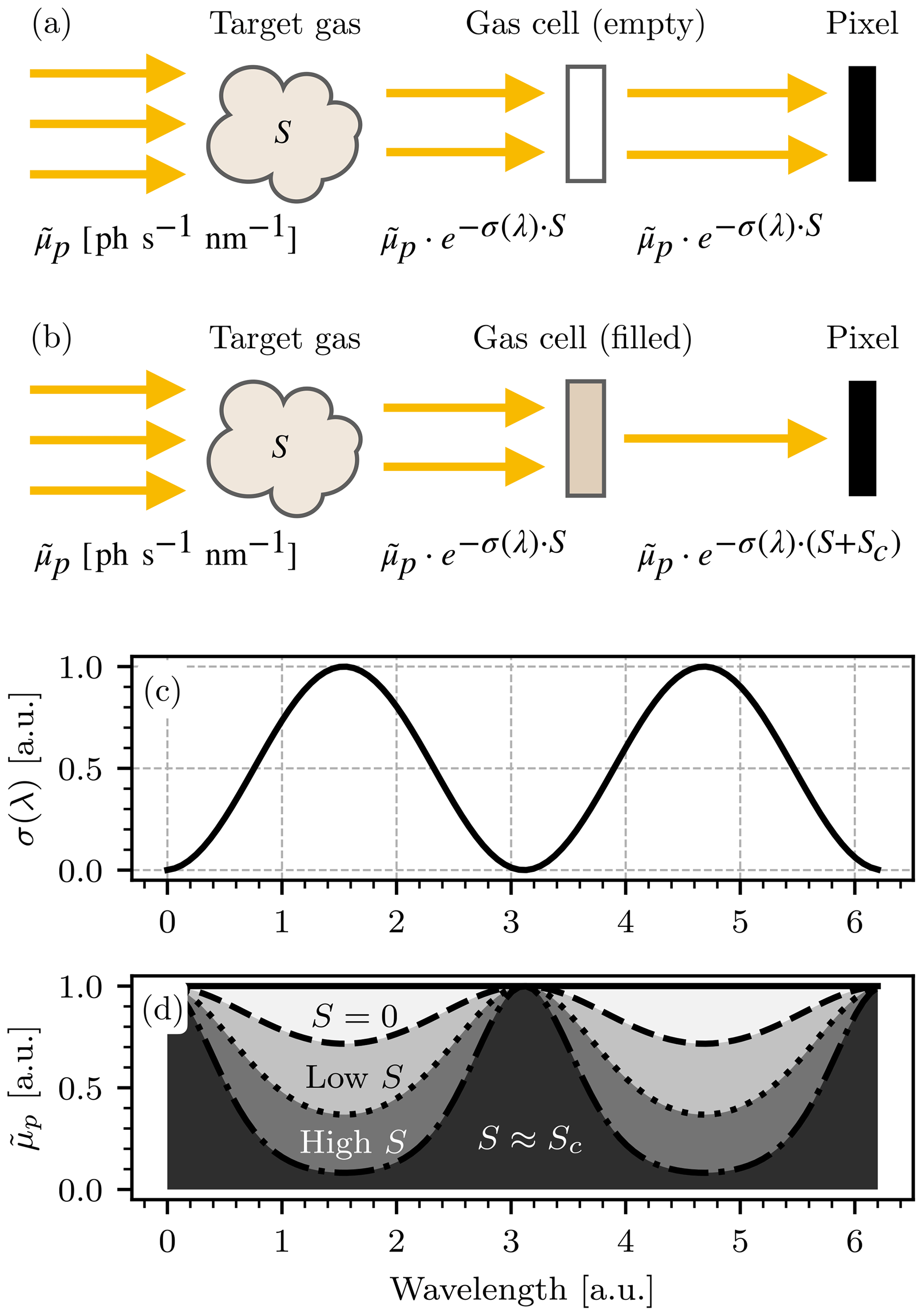
Figure 2 Schematic depiction of the absorption of incoming light in a GCS-based instrument. For simplicity only a single absorber is assumed. (a) The absorption scheme for the channel with the empty cell. (b) The absorption scheme for the channel with the filled cell. S denotes the column density of the target gas and S_c the column density of the target species in the gas cell of the instrument. Panels (c) and (d) demonstrate the principle of GCS: given a hypothetical absorption cross section (here assumed to be of sinusoidal shape, displayed in c), the spectral absorption can be derived from the Lambert–Beer law for different choices of S (here S=0, “low S”, “high S”). A photosensor is only sensitive to the spectrally integrated radiance that it is exposed to, i.e., the gray-colored areas displayed in (d).

For a detector pixel with the indices (i,j), the camera with the empty cell will measure

$$\begin{array}{}\text{(7)}& J_{(i,j)}=\underset{\mathrm{0}}{\overset{t_{\exp }}{\int }}\underset{\mathrm{0}}{\overset{\mathrm{\infty }}{\int }}\mathit{\eta }\left(\mathit{\lambda }\right)\cdot {\stackrel{\mathrm{̃}}{\mathit{\mu }}}_{\mathrm{p}}\cdot e^{-\mathit{\sigma }\left(\mathit{\lambda }\right)\cdot S_{(i,j)}}\mathrm{d}\mathit{\lambda }\mathrm{d}t,\end{array}$$

and the camera with the cell containing the target gas will measure

$$\begin{array}{}\text{(8)}& J_{c,(i,j)}=\underset{\mathrm{0}}{\overset{t_{\exp }}{\int }}\underset{\mathrm{0}}{\overset{\mathrm{\infty }}{\int }}\mathit{\eta }\left(\mathit{\lambda }\right)\cdot {\stackrel{\mathrm{̃}}{\mathit{\mu }}}_{\mathrm{p}}\cdot e^{-\mathit{\sigma }\left(\mathit{\lambda }\right)\cdot (S_{(i,j)}+S_{\mathrm{c}})}\mathrm{d}\mathit{\lambda }\mathrm{d}t,\end{array}$$

where S_(i,j) denotes the column density of the target gas in the FOV of the pixel with indices (i,j) and S_c the column density of the target gas in the gas cell of the instrument. The two measurements J_(i,j) and $J_{c,(i,j)}$ can be interpreted as spectral channels in analogy to the widely used DOAS terminology. In imaging GCS, the instrument response (instrument signal),

$$\begin{array}{}\text{(9)}& {\stackrel{\mathrm{̃}}{\mathit{\tau }}}_{(i,j)}=\ln \left(J_{c,(i,j)}/J_{(i,j)}\right),\end{array}$$

is computed for each individual pixel. ${\stackrel{\mathrm{̃}}{\mathit{\tau }}}_{(i,j)}$ is the logarithmic signal ratio between the two spectral channels of the instrument and functions as a measure of S_(i,j): when S_(i,j) is small, incoming light will be only slightly attenuated before it reaches the cells, and thus the signal ratio $J_{c,(i,j)}/J_{(i,j)}$ will be smaller compared to a scenario in which S_(i,j) is large, and thus the atmospheric target gas has already attenuated a larger portion of the light that would otherwise have been absorbed by the gas cell. It therefore follows directly that ${\stackrel{\mathrm{̃}}{\mathit{\tau }}}_{(i,j)}$ grows monotonically with S_(i,j).

When using two camera modules with distinct optical setups, the resulting detector signals are highly sensitive to imperfections in the optical path. For example, small differences in the focal lengths of the camera lenses or dust particles on the lenses or gas cells can induce significant false signals, contributing to $\stackrel{\mathrm{̃}}{\mathit{\tau }}$. Furthermore, vignetting is immanent to imaging measurements and manifests itself in increasing false signal gradients towards the corners of the image. Even with entirely identical optical setups, the two camera sensors may have slightly different pixel response nonuniformity (PRNU) maps. These effects can be partly corrected by recording reference signals $J_{\mathrm{ref},(i,j)}$ for the channel with the empty cell and $J_{c,\mathrm{ref},(i,j)}$ for the channel with the filled cell in the zenith direction, where S=0 is assumed. In reality this latter condition does not need to be perfectly fulfilled, although it is important that S is approximately constant throughout the FOV for the reference images. In analogy to Eqs. (7) and (8) the reference signals are given by

$$\begin{array}{}\text{(10)}& J_{\mathrm{ref},(i,j)}=\underset{\mathrm{0}}{\overset{t_{\exp }}{\int }}\underset{\mathrm{0}}{\overset{\mathrm{\infty }}{\int }}\mathit{\eta }\left(\mathit{\lambda }\right)\cdot {\stackrel{\mathrm{̃}}{\mathit{\mu }}}_{\mathrm{p}}\mathrm{d}\mathit{\lambda }\mathrm{d}t\end{array}$$

and

$$\begin{array}{}\text{(11)}& J_{c,\mathrm{ref},(i,j)}=\underset{\mathrm{0}}{\overset{t_{\exp }}{\int }}\underset{\mathrm{0}}{\overset{\mathrm{\infty }}{\int }}\mathit{\eta }\left(\mathit{\lambda }\right)\cdot {\stackrel{\mathrm{̃}}{\mathit{\mu }}}_{\mathrm{p}}\cdot e^{-\mathit{\sigma }\left(\mathit{\lambda }\right)\cdot S_{\mathrm{c}}}\mathrm{d}\mathit{\lambda }\mathrm{d}t.\end{array}$$

The measurement signal ratio is then divided by the reference signal ratio, i.e.,

$$\begin{array}{}\text{(12)}& {\stackrel{\mathrm{̃}}{\mathit{\tau }}}_{(i,j)}=\ln \left({\displaystyle \frac{J_{c,(i,j)}\cdot J_{\mathrm{ref},(i,j)}}{J_{(i,j)}\cdot J_{c,\mathrm{ref},(i,j)}}}\right).\end{array}$$

This procedure is also referred to as flat-field correction. In the following section it will be shown that in good approximation $\stackrel{\mathrm{̃}}{\mathit{\tau }}\propto S$ holds.

Furthermore, Eq. (12) points towards a crucial benefit of the proposed measurement principle. While other correlation methods for remote sensing typically operate with two channels in different spectral domains (e.g., an on- and off-band channel in filter-spectroscopy-based SO₂ cameras), the spectral domain of the two channels is identical in GCS. Additionally, that domain is typically restricted to a few dozen nanometers using a bandpass filter. This makes the instrument insensitive to broadband extinction, i.e., by Rayleigh scattering or due to aerosols, given that their extinction coefficients vary only very slightly throughout the spectral domain the instrument operates in. The instrument response to broadband extinction is examined numerically in Sect. 2.2.

2.2 Instrument model calculation

Figure 3 (a) The absorption cross section of NO₂. The red filled region marks the transmission region of the bandpass filter used in our instrument. The inset in the top right shows a zoomed-in view of a spectral range that contains the filter transmission and shows highly structured absorption features. (b) The radiance spectrum, as well as the transmission lines of the filter T_f and the lens T_l, the quantum efficiency of the camera sensor η, and the total throughput $T_{\mathrm{f}}\cdot T_{\mathrm{l}}\cdot \mathit{\eta }$ that are assumed in the instrument model.

A numerical forward model was implemented to predict the characteristics of a GCS-based NO₂ camera. Specifically, we investigate the shape of the instrument response, the calibration curve, and the signal-to-noise ratio (SNR) as a function of S and S_c, as well as cross-sensitivities to other atmospheric trace gases. This section specifically discusses the application of GCS to measurements of NO₂. Other trace gases may, for example, require operating in a different spectral range. Overall, the simulation of realistic conditions of daytime measurements in the atmosphere is the aim. For this, a spectrum of scattered sunlight is used as the light source and atmospheric NO₂ column densities are considered in the range from 10¹⁶ to 10¹⁸ molec. cm⁻², as well as integration times on the scale of seconds. The assumed range of NO₂ column densities is justified as follows: in order to measure column densities much lower than 10¹⁶ molec. cm⁻², the exposure time would need to be increased significantly, resulting in poor temporal resolution. At the same time, even strong NO₂ pollution in the atmosphere typically does not exceed 10¹⁸ molec. cm⁻², assuming realistic viewing geometries.

The relevant detector signals are modeled according to Eqs. (7), (8), (10), and (11). In this instrument model, we assume $T\left(\mathit{\lambda }\right)=T_{\mathrm{f}}\left(\mathit{\lambda }\right)\cdot T_{\mathrm{l}}\left(\mathit{\lambda }\right)$, where T_f denotes the transmission of the bandpass filter and T_l denotes the transmission of the camera lens. Since t_exp is realistically small enough that I₀(λ) is constant throughout exposure and the transmission of the bandpass filter used is effectively a cutoff function outside its transmission band from 430 to 445 nm, the detector signals can be simplified to

$$\begin{array}{}\text{(13)}& J\left(\mathit{\tau }\right)=t_{\exp }\cdot \underset{\mathrm{430}\mathrm{nm}}{\overset{\mathrm{445}\mathrm{nm}}{\int }}\mathit{\eta }\left(\mathit{\lambda }\right)\cdot {\stackrel{\mathrm{̃}}{\mathit{\mu }}}_{\mathrm{p}}\left(\mathit{\lambda }\right)\cdot e^{-\mathit{\tau }}\mathrm{d}\mathit{\lambda }.\end{array}$$

The choice of this particular bandpass filter is motivated by the strong, characteristic absorption features that NO₂ shows in its transmission range. The absorption cross section of NO₂ (Vandaele et al., 2002) is displayed in Fig. 3a with a zoomed-in region close to the transmission band of the bandpass filter.

The model requires a light source radiance spectrum L₀. For realistic applications of the instrument the light source will almost exclusively be an atmospheric background spectrum, i.e., a radiance spectrum of scattered sunlight. We use a highly resolved irradiance spectrum in units of W nm⁻¹ m⁻² (Chance and Kurucz, 2010) and scale it with a low-resolution radiance spectrum at 400 nm (Pissulla et al., 2009) in units of W nm⁻¹ m⁻² sr⁻¹. This way we obtain a radiance spectrum that represents the typical spectral shape of scattered sunlight but maintain the high spectral resolution of the irradiance spectrum. We argue that this is the most realistic general estimation of the background spectrum that we can make. The radiance spectrum used for scaling was recorded at Thessaloniki, Greece, at a sun zenith angle of 21^∘. The transmission lines of the bandpass filter T_f(λ) and the camera lenses T_l(λ), as well as the quantum efficiency of the camera sensors η(λ), are provided by the manufacturers. An étendue of $E\approx {\mathrm{10}}^{-\mathrm{5}}$ sr mm² was assumed throughout, which was computed on the basis of a fully opened aperture (f number 1.6). Figure 3b shows plots of L₀, T_f, T_l, and η. In the following we assume an exposure time of 2 s. The detector signals J, J_c, J_ref, and J_c,ref are then calculated by numeric integration, according to the instrument model as described. Figure 4 shows the modeled instrument response $\stackrel{\mathrm{̃}}{\mathit{\tau }}$ (see Eq. 12) as a function of the column density S in the range from 10¹⁶ to 10¹⁸ molec. cm⁻² for different choices of the column density S_c inside the NO₂ cell of the instrument.

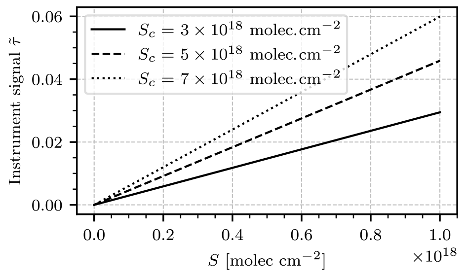
Figure 4 The modeled instrument signal $\stackrel{\mathrm{̃}}{\mathit{\tau }}=\ln \left(J_c\cdot J_{\mathrm{ref}}/\left(J\cdot J_{c,\mathrm{ref}}\right)\right)$ as a function of the target gas column density S for different choices of cell column density S_c. The instrument response is almost perfectly linear in S. The slope of each line yields the instrument calibration corresponding to S_c.

The instrument response is in good approximation proportional to S. The instrument calibration factor k can be obtained for any fixed value of S_c by sampling the instrument signal $\stackrel{\mathrm{̃}}{\mathit{\tau }}$ for different choices of S and fitting a linear function of the form

$$\begin{array}{}\text{(14)}& \stackrel{\mathrm{̃}}{\mathit{\tau }}\left(S\right)=k\left(S_{\mathrm{c}}\right)\cdot S\end{array}$$

to the samples. In order to convert the unitless instrument signal $\stackrel{\mathrm{̃}}{\mathit{\tau }}$ to column densities, the inverse k⁻¹(S_c) in units of molec. cm⁻² is used. During measurements, S_c must be determined so that k⁻¹(S_c) can be computed. For this purpose, S_c could be directly measured using a second instrumental setup, such as a DOAS instrument. However, in many measuring scenarios it is more practical to determine S_c on the basis of the acquired images alone. For this purpose, an off-plume region of the imaged scene, where S=0 is assumed, is used, and S_c is approximated by

$$\begin{array}{}\text{(15)}& S_{\mathrm{c}}=\ln \left(J/J_c\right)/\stackrel{\mathrm{‾}}{\mathit{\sigma }},\end{array}$$

where $\stackrel{\mathrm{‾}}{\mathit{\sigma }}\approx \mathrm{5.1}\cdot {\mathrm{10}}^{-\mathrm{19}}$ cm² molec.⁻¹ is the absorption cross section of NO₂ averaged over the spectral range from 430 to 445 nm. The validity of this approximation was verified numerically, as displayed in Fig. 5. For a cell column density of $S_{\mathrm{c}}=\mathrm{4}\cdot {\mathrm{10}}^{\mathrm{18}}$ molec. cm⁻² (this value will be reasoned in the following paragraph), the proposed approximation underestimates the true value of S_c by less than 2⋅10¹⁷ molec. cm⁻².

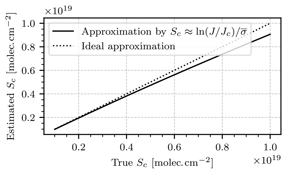
Figure 5 The S_c approximation in Eq. (15) as a function of the true values of S_c. For $S_{\mathrm{c}}=\mathrm{4}\cdot {\mathrm{10}}^{\mathrm{18}}$ molec. cm⁻², the proposed approximation underestimates the true value of S_c by less than 2⋅10¹⁷ molec. cm⁻².

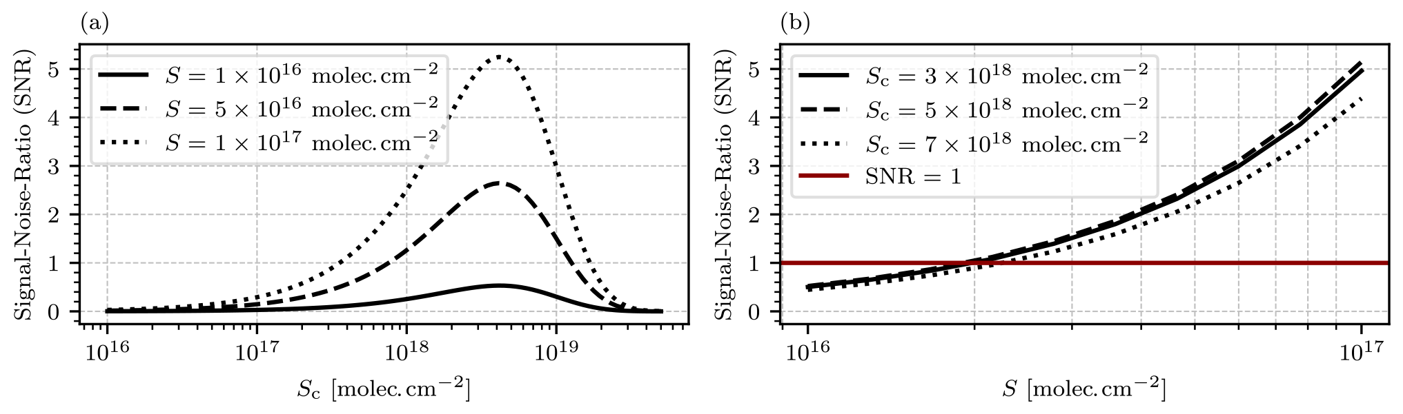
Figure 6 (a) Modeled SNR as a function of the cell column density S_c for different choices of the target gas column density S. The highest SNR is reached for a cell column density of approximately $S_{\mathrm{c}}\approx \mathrm{4}\cdot {\mathrm{10}}^{\mathrm{18}}$ molec. cm⁻², with a slight dependence on S. (b) Modeled SNR as a function of the column density of the target gas S for different choices of the cell gas column density S_c. The red vertical line marks SNR=1 and thus the detection limit of the instrument.

With this model we can also quantify the signal-to-noise ratio (SNR) in order to estimate the detection limit of the instrument under typical atmospheric conditions. An SNR of 1 is assumed to be the lower limit at which atmospheric column densities of the target gas can be resolved. Photoelectron counting follows Poissonian statistics; i.e., the uncertainty ΔJ of a signal measured by a photosensor is $\mathrm{\Delta }J=\sqrt{J}$. Thus, the uncertainty $\mathrm{\Delta }\stackrel{\mathrm{̃}}{\mathit{\tau }}$ of the instrument signal $\stackrel{\mathrm{̃}}{\mathit{\tau }}$ can be expressed in closed form by application of Gaussian uncertainty propagation:

$$\begin{array}{}\text{(16)}& \mathrm{\Delta }\stackrel{\mathrm{̃}}{\mathit{\tau }}={\displaystyle \frac{\mathrm{1}}{\left(\sqrt{\mathrm{1}/J+\mathrm{1}/J_c+\mathrm{1}/J_{\mathrm{ref}}+\mathrm{1}/J_{c,\mathrm{ref}}}\right)}}.\end{array}$$

In practice the uncertainties of the reference signals will be comparably small because the exposure time for the recording of J_ref and J_c,ref can be chosen to make the contribution of $\mathrm{1}/J_{\mathrm{ref}}$ and $\mathrm{1}/J_{c,\mathrm{ref}}$ negligible. Then the uncertainty reduces to

$$\begin{array}{}\text{(17)}& \mathrm{\Delta }\stackrel{\mathrm{̃}}{\mathit{\tau }}={\displaystyle \frac{\mathrm{1}}{\sqrt{\left(\mathrm{1}/J+\mathrm{1}/J_c\right)}}},\end{array}$$

and the SNR can be expressed as

$$\begin{array}{}\text{(18)}& \mathrm{SNR}={\displaystyle \frac{\stackrel{\mathrm{̃}}{\mathit{\tau }}}{\mathrm{\Delta }\stackrel{\mathrm{̃}}{\mathit{\tau }}}}={\displaystyle \frac{\ln \left(J_c/J\right)-\ln \left(J_{c,\mathrm{ref}}/J_{\mathrm{ref}}\right)}{\sqrt{\left(\mathrm{1}/J+\mathrm{1}/J_c\right)}}}.\end{array}$$

This instrument model only accounts for the photon shot noise and disregards additional possible sources of noise such as dark noise and read-out noise of the photosensors. This is on purpose in order to make the model applicable to different instrumental setups. In practice the shot noise is by far the dominating source of noise due to the large light throughput of the setup, and both dark current and dark noise can be neglected (see Sect. 3 for a more detailed explanation). Figure 6a shows the modeled SNR as a function of the cell column density S_c for different choices of the column density of the target gas S. The highest SNR is reached at approximately $S_{\mathrm{c}}\approx \mathrm{4}\cdot {\mathrm{10}}^{\mathrm{18}}$ molec. cm⁻² with a slight dependence on the observed target gas column density S. Figure 6b shows the modeled SNR as a function of the target gas column density S. The red horizontal line marks the resulting detection limit, with SNR=1. With an ideal choice of $S_{\mathrm{c}}\approx \mathrm{4}\cdot {\mathrm{10}}^{\mathrm{18}}$ molec. cm⁻², a detection limit of approximately 2⋅10¹⁶ molec. cm⁻² is reached with an exposure time of 2 s.

The instrument model also allows for the study of the selectivity of the instrument. Equation (13) holds under the assumption that the target gas is the sole absorber. In a realistic measuring scenario many different trace gases other than NO₂ could be present in the atmosphere. Cross-sensitivities to other trace gases can be determined on the basis of the instrument model. We define ${\stackrel{\mathrm{̃}}{\mathit{\tau }}}_X$, the false signal of a species X, as the additional contribution to the overall instrument signal $\stackrel{\mathrm{̃}}{\mathit{\tau }}$ that is due to the absorption of X and present the results of a study on the false signals of water vapor (H₂O; absorption cross section was taken from Rothman et al., 2013) and the oxygen collision complex (O₄; absorption cross section was taken from Thalman and Volkamer, 2013), since both species show possibly relevant absorption features in the spectral range our instrument operates in. Figure 7 shows the absorption cross sections of NO₂, H₂O, O₄, and the transmission line of the bandpass filter used.

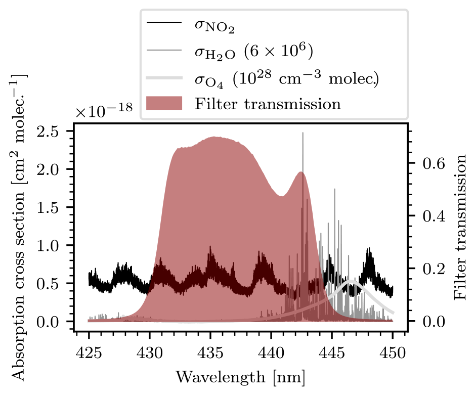
Figure 7 Cross sections of NO₂, H₂O, and O₄, as well as the transmission of the bandpass filter (red shaded area) used. The cross sections of H₂O and O₄ were scaled (see legend) in order to display them on a mutual axis.

The bandpass filter blocks almost all light of wavelengths greater than λ=445 nm. Therefore, most of the O₄ absorption is filtered out and ${\stackrel{\mathrm{̃}}{\mathit{\tau }}}_{{\mathrm{O}}_{\mathrm{4}}}$ is strongly reduced. Water vapor, on the other hand, shows strong absorption features between 440 and 445 nm. Calculating the false signals of the two species requires an assumption of their atmospheric abundance. In reality these column densities can vary strongly with place and time. We therefore use the model to make predictions of the cross-sensitivities assuming large but still realistic column densities of the cross-sensitive species. If the predicted false signals are sufficiently small, the cross-sensitivities can be neglected altogether because the model has then realistically overestimated the induced false signals. For O₄ a maximum column density of 10⁴⁴ molec.² cm⁻⁵ at a light path length of 10 km was assumed. For reference, Peters et al. (2019) report maximal O₄ column densities of around 5⋅10⁴³ molec.² cm⁻⁵ during the CINDI-2 measurement campaign. For H₂O a maximum column density of 6⋅10²³ molec. cm⁻² was assumed. This corresponds to a relative humidity of 100 % at a pressure of 1 atm, temperature of 20^∘ C, and a light path length of 10 km.

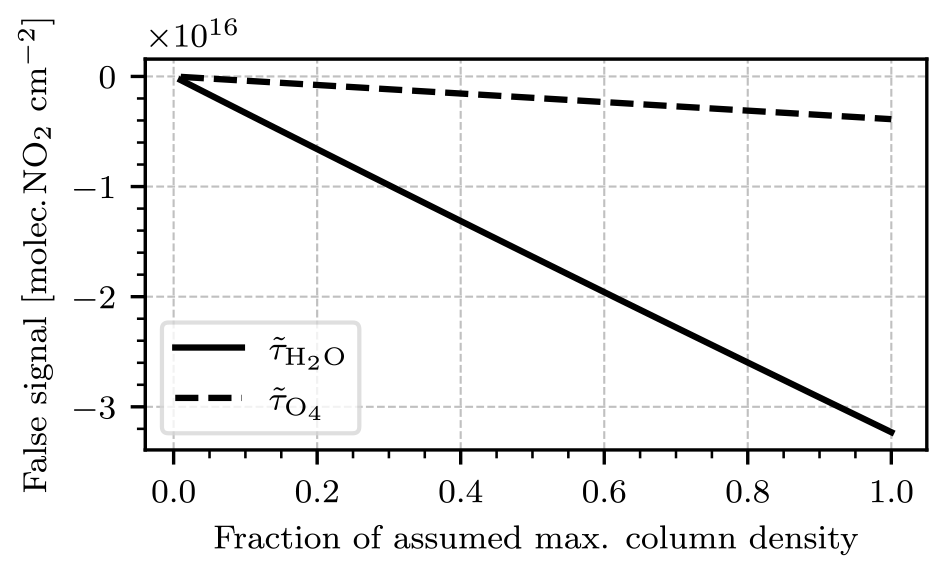
Figure 8 Modeled cross-sensitivity to H₂O and O₄. The ordinate shows the fraction of the assumed maximal column density for both species, which are 6⋅10²³ molec. cm⁻² for H₂O and 10⁴⁴ molec.² cm⁻⁵ for O₄. The abscissa shows the false signal of the two species converted to NO₂ column density equivalents. The calibration of the model was obtained from Fig. 4, assuming a column density of $S_{\mathrm{c}}=\mathrm{4}\cdot {\mathrm{10}}^{\mathrm{18}}$ molec. cm⁻² in the gas cell.

Figure 8 shows the modeled false signals of H₂O and O₄. The false signal was converted to NO₂ column density equivalents using the calibration of the model obtained from Fig. 4, assuming a cell column density of $S_{\mathrm{c}}=\mathrm{4}\cdot {\mathrm{10}}^{\mathrm{18}}$ molec. cm⁻². Both species induce a negative false signal. When expressed in NO₂ signal equivalents, the false signal of O₄ is comparably small, reaching around $-\mathrm{2}\cdot {\mathrm{10}}^{\mathrm{15}}$ molec. cm⁻² assuming the maximal column. The false signal of H₂O is an order of magnitude larger, reaching up to $-\mathrm{3.2}\cdot {\mathrm{10}}^{\mathrm{16}}$ molec. cm⁻² assuming the maximal column. As discussed, we treat these false signals and the column densities that have generated them as an overestimate of a realistic expectation. In addition, the naturally abundant water vapor of the atmosphere is typically distributed much more homogeneously than strong NO₂ concentration gradients from a point source. Under this circumstance any false signal induced by water vapor should be easily separable from the NO₂ signal of interest. Water vapor inside the plume of a point source emission, which cannot be separated from the NO₂ signal by the argument above, is contained within much shorter light paths (typically on the order of 100–200 m) and is not expected to induce relevant false signals.

In addition to water vapor and O₄ the modeled instrument response to broadband extinction was investigated. Rayleigh scattering has a wavelength dependence of λ⁻⁴, while extinction due to larger particles shows weaker wavelength dependence. It was verified in a numerical experiment that the instrument response curves displayed in Fig. 4 vary by less than 0.5 % when the assumed irradiance spectra are scaled by λ⁻⁴ and λ⁰=1. This demonstrates that the GCS-based NO₂ camera is practically insensitive to broadband extinction. Beside the numeric model presented here, an analytic model was developed as well (see Appendix A).

3 Instrument prototype

We have built an instrument prototype based on commercially available hardware. The camera modules use a monochrome progressive-scan CMOS sensor in a $\mathrm{1}/\mathrm{1.2}$ in. format with a pixel size of 5.86 µm×5.86 µm and a global shutter. They record images with 1920×1200 (height × width) pixels. A charge signal is digitized by a 16-bit analog–digital converter (ADC). The cameras connect via USB 3 to a controlling computer equipped with corresponding camera software. Image acquisition rates depend on the selected exposure time and the read-out time t_read=24.4 ms of the camera sensors. The instrument is therefore limited to a frame rate of 41 FPS at best. However, the read-out time t_read can be reduced by using windowing, a feature in which the cameras are advised to only read out a subrange of their sensor arrays. The usability of windowing depends on the imaged scene and whether large parts of the FOV can be neglected. The camera modules have a read-out noise of 7 e⁻. The thermal dark signal of the camera modules was determined experimentally according to the European Machine Vision Association (EMVA) (see Jähne, 2010). A thermal dark signal of (24±9) e⁻ s⁻¹ at a sensor temperature of 50 ^∘C, which is approximately the average operating temperature of the camera modules due to their small form factor, and a doubling temperature of (6.1±0.1) ^∘C were found. The camera modules have a full-well depth of 34 000 e⁻. Given that in bright daylight the exposure times for images within the dynamic range of the camera are typically far below 1 s, the contribution of the dark signal to the total measured camera signal is negligibly small (e.g., below 0.05 % for an exposure time of 30 ms and a sensor saturation of 50 %). Also, the total dark noise (meaning read-out noise + thermal noise) is negligible compared to the photon shot noise of around 130 e⁻ at 50 % saturation. From a technical perspective the retrieval of the camera data follows the typical pattern of digital imaging: inside the camera modules, the incoming photons detach electrons from the semiconductor material of the camera chip (characterized by η). That charge is digitized (characterized by the fixed ADC gain K in units of e⁻ ph⁻¹) and saved as 16-bit grayscale image files. Each camera is equipped with a lens with a focal length of f=25 mm. The full diagonal, vertical, and horizontal opening angles amount to 30, 16, and 25.5^∘, respectively. For each camera a bandpass filter with transmission in the range from 430–445 nm was placed between the camera lens and the camera sensor. The gas cells of the instrument are cylindrical with a diameter of 50 nm and a thickness of 10 nm. The NO₂ cell was filled from a large reservoir to contain an NO₂ column density of 4⋅10¹⁸ molec. cm⁻² (which is the ideal value according to the results shown in Sect. 2.2, specifically Fig. 6a). The camera behind the NO₂ cell is mounted to a tiltable stage, which can be used to adjust its optical axis in vertical and horizontal orientation with milliradian (mrad) precision using two thumb screws. This adjustment is of crucial importance in order to eliminate shifts in the FOVs of the two cameras. All parts are placed inside a closable plastic case. Overall, the instrument is portable and compact while maintaining a reasonable cost of below EUR 2000. Control software with graphical user interface was developed in the Python programming language.

4 Measurements

4.1 Proof-of-concept measurement with gas cells

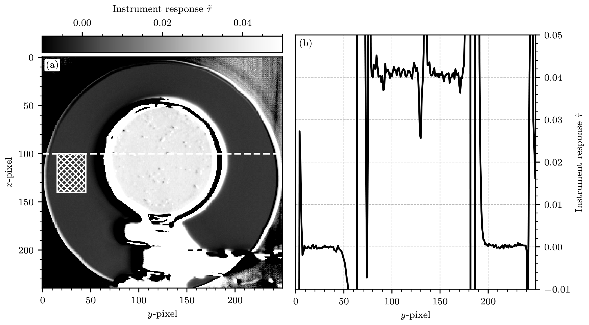
Figure 9 (a) The processed camera image for reference cell no. 4. The cell is in the center of the image. The circular structure behind it is the opening of the integrating sphere, in which a halogen lamp is placed as the light source of the experiment. The foreground shows the stand and clamp that are used to hold the cell in front of the integrating sphere. The in-cell region of the test cell shows a larger instrument signal than the background. The background region of our choice is marked with a patterned rectangle (left of the cell). (b) The instrument signal plotted along a vertical cross section through the middle of the test cell at x=100 (see the dashed line in a). The region in the middle shows the enhanced signal within the cell. The strong peaks separating the background region and the in-cell region are generated by the frame of the cell. The strong structure that can be seen in the middle of the cell at around y=130 is due to condensation on the inside of the cell or similar imperfections of the experimental setup.

In order to validate the instrument model described in Sect. 2.2 a simple laboratory experiment was performed. Four glass cells were filled with different concentrations of NO₂ and measured with both the NO₂ camera and a conventional DOAS setup. The light source for the camera measurement was a halogen lamp inside an integrating sphere in front of which the cells were mounted onto a stand with a clamp. An additional series of images was recorded without a cell in the light path, whose average serves as the reference image (J_ref, J_c,ref; see Eq. 12). When evaluating the images taken by the NO₂ camera, an in-cell pixel set and a background pixel set were defined. The in-cell pixel set contained the pixels inside the cell, while the background pixel set contained pixels of the illuminated entrance of the integrating sphere, not covered by the cell. Due to the varying size of the test cells, the in-cell and background pixel sets were different for each cell. The total acquisition time of the NO₂ camera was set to 3 min for each cell, and the exposure time of each camera was chosen such that the camera sensors saturated to approximately 50 %.

First, the column density inside the gas cell of the NO₂ camera was estimated as

$$\begin{array}{}\text{(19)}& S_{\mathrm{c}}=\ln \left(\stackrel{\mathrm{‾}}{J_{\mathrm{bg}}}/\stackrel{\mathrm{‾}}{J_{c,\mathrm{bg}}}\right)/\stackrel{\mathrm{‾}}{\mathit{\sigma }},\end{array}$$

where $\stackrel{\mathrm{‾}}{J_{\mathrm{bg}}}$ and $\stackrel{\mathrm{‾}}{J_{c,\mathrm{bg}}}$ are the camera signals of the camera with the empty cell and the one with the filled cell, respectively, averaged over the background pixels of all images. $\stackrel{\mathrm{‾}}{\mathit{\sigma }}\approx \mathrm{5.1}\cdot {\mathrm{10}}^{-\mathrm{19}}$ cm² molec.⁻¹ is the absorption cross section of NO₂ averaged over the spectral range from 430 to 445 nm. A cell column density of $S_{\mathrm{c}}=(\mathrm{3.89}\pm \mathrm{0.03})\cdot {\mathrm{10}}^{\mathrm{18}}$ molec. cm⁻² was obtained. The cell was originally filled with $S_{\mathrm{c}}=\mathrm{4}\cdot {\mathrm{10}}^{\mathrm{18}}$ molec. cm⁻², but this deviation can be explained by the temperature-dependent NO₂ ⇌ N₂O₄ equilibrium. The lower the temperature, the lower the NO₂ concentration inside the gas cell. The calibration of the instrument was obtained from the instrument model as explained in Sect. 2.2. The fit procedure yielded a calibration factor of $k^{-\mathrm{1}}=(\mathrm{2.69}\pm \mathrm{0.02})\cdot {\mathrm{10}}^{\mathrm{19}}$ molec. cm⁻². Additionally, the signal offset ${\stackrel{\mathrm{̃}}{\mathit{\tau }}}_{\mathrm{0}}$ of the instrument was calculated from the background pixels, which was defined as

$$\begin{array}{}\text{(20)}& {\stackrel{\mathrm{̃}}{\mathit{\tau }}}_{\mathrm{0}}=\ln \left(\stackrel{\mathrm{‾}}{J_{c,\mathrm{bg}}}/\stackrel{\mathrm{‾}}{J_{\mathrm{bg}}}\right).\end{array}$$

Subtraction of ${\stackrel{\mathrm{̃}}{\mathit{\tau }}}_{\mathrm{0}}$ from the instrument signal $\stackrel{\mathrm{̃}}{\mathit{\tau }}$ set the average background pixel to zero. The instrument signal of a test cell was determined by averaging over the pixels that were covered by the cell, i.e.,

$$\begin{array}{}\text{(21)}& \stackrel{\mathrm{̃}}{\mathit{\tau }}=\ln \left(\stackrel{\mathrm{‾}}{J_c}/\stackrel{\mathrm{‾}}{J}\right),\end{array}$$

where J and J_c denote the camera signal with the empty cell and with the filled gas cell, respectively, in the in-cell pixel region.

Table 1 Column densities and instrument signal $\stackrel{\mathrm{̃}}{\mathit{\tau }}$ of each reference cell measured with a DOAS instrument and the NO₂ camera.

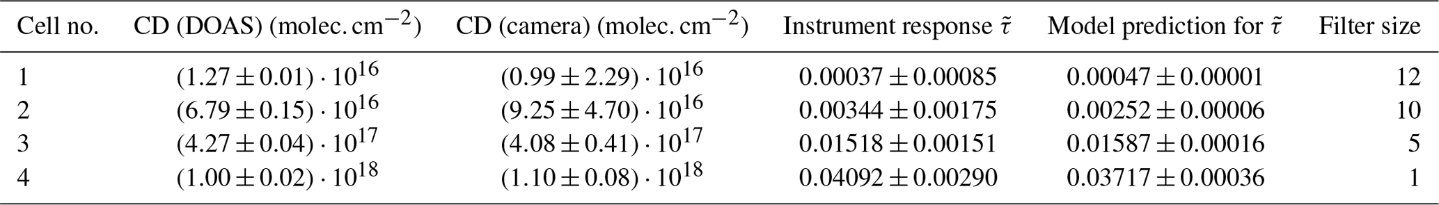
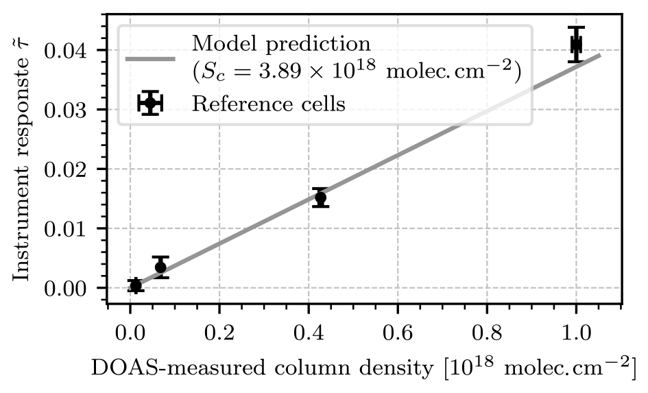
Figure 10 Scatter plot of the instrument response $\stackrel{\mathrm{̃}}{\mathit{\tau }}$ against the DOAS-measured column density of each test cell. The gray line shows the prediction of the instrument model with cell column density $S_{\mathrm{c}}=\mathrm{3.89}\cdot {\mathrm{10}}^{\mathrm{18}}$ molec. cm⁻².

The uncertainty of these measurements is given by Gaussian error propagation according to Eq. (17). The uncertainties $\mathrm{\Delta }\stackrel{\mathrm{‾}}{J_c}$ and $\mathrm{\Delta }\stackrel{\mathrm{‾}}{J}$ are obtained by computing the standard deviation of the detector signal in the in-cell region for the two channels, respectively. Figure 9a shows an exemplary image of this measurement. In the center foreground of the image the outline of test cell no. 4 as well as the stand and clamp used to hold it are shown. The offset ${\stackrel{\mathrm{̃}}{\mathit{\tau }}}_{\mathrm{0}}$ was subtracted and the flat-field correction was applied using the reference images according to Eq. (12). The camera measured a signal of $\stackrel{\mathrm{̃}}{\mathit{\tau }}=(\mathrm{4.092}\pm \mathrm{0.290})\cdot {\mathrm{10}}^{-\mathrm{2}}$ in the in-cell region of the test cell. Using the calibration factor k⁻¹, a column density of $S=(\mathrm{1.10}\pm \mathrm{0.08})\cdot {\mathrm{10}}^{\mathrm{18}}$ molec. cm⁻² was obtained. Within the uncertainty of the measurement this result coincides with that of the DOAS instrument, which measured a column density of $S=(\mathrm{1.00}\pm \mathrm{0.02})\cdot {\mathrm{10}}^{\mathrm{18}}$ molec. cm⁻².

Table 1 lists the column densities measured for each cell by the DOAS setup and the NO₂ camera. The measurements taken with the NO₂ camera show significant uncertainties. For cell no. 1, the relative uncertainty is as large as 230 % and the detection limits, ranging from 2.29⋅10¹⁶ molec. cm⁻² to 8⋅10¹⁶ molec. cm⁻², are larger than the prediction of the instrument model, which was 2⋅10¹⁶ molec. cm⁻² at 2 s of exposure. The reason for this deviation is the use of a different light source: while the instrument model assumed scattered sunlight as the light source, a halogen lamp inside an integrating sphere was used for this experiment. The detection limit is mainly determined by the overall intensity of the light source, which is much lower for such a halogen lamp in the blue spectral range. This increased the statistical uncertainty of the measurement. Additionally, systematic false signals were observed, which were not considered in the instrument model: due to the small diameter of the test cells and the limited interior space of typical optical laboratories there are inevitable perspective shifts between the images of the two cameras when they are oriented so that the test cells are in the center of their FOVs. Small dust particles on the test cell or condensed droplets on its inside can then introduce false signals. In order to smooth out these false signals, the images were convoluted with a rectangle filter of the same size as the average diameter of the observed structures. Table 1 lists the chosen filter size for each cell. The filter sizes were chosen differently for each cell because the larger cells required less smoothing. The cell image shown in Fig. 9 required no smoothing at all (which corresponds to a filter size of 1 pixel). Figure 10 shows a scatter plot of the instrument response of the NO₂ camera against the column density measured with the DOAS setup for each test cell. Additionally, the prediction of the instrument model (see Sect. 2.2) with cell column density $S_{\mathrm{c}}=\mathrm{3.89}\cdot {\mathrm{10}}^{\mathrm{18}}$ molec. cm⁻² is plotted. The resulting instrument responses to the test cells are in very good agreement with the instrument model, with an average relative deviation of 18 %. The model and measurement coincide for all test cells within the uncertainties of the measurement. Given the overall good agreement between the DOAS instrument, the NO₂ camera, and the instrument model, we take these results as proof of concept.

4.2 Measuring the emissions of the coal power plant Großkraftwerk Mannheim

4.2.1 Setup and methodology

We report measurements taken at the Großkraftwerk Mannheim (GKM) with the NO₂ camera. The GKM is a power plant located in Mannheim, Germany, which generates electricity based on burning of bituminous coal. It is one of the largest power suppliers of southwestern Germany. The European Pollutant Release and Transfer Register (E-PRTR) lists an emission of 2 890 000 kg of NO_x in 2017 (The European Commision, 2017).

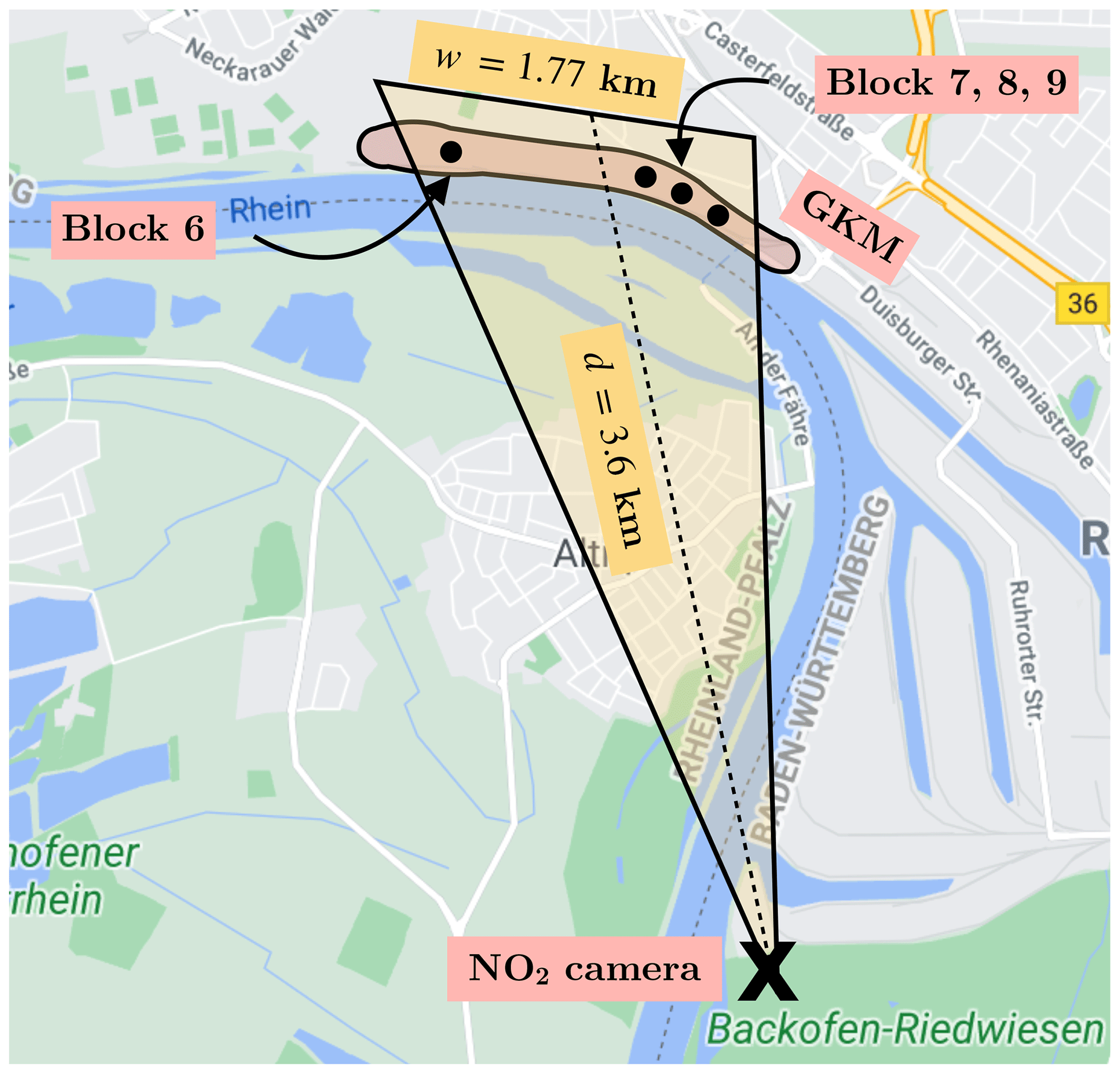
Figure 11 The GKM measurement in bird's-eye perspective (© Google Maps 2021). The NO₂ camera was set up at Backofen-Riedwiesen, 3.6 km south of the GKM, and positioned so that the emission of block 7 was in the middle of the FOV.

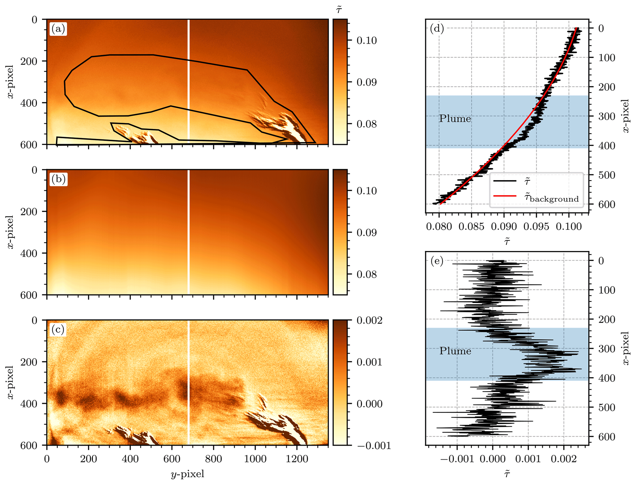
Figure 12 (a) Camera image of the GKM measurement (26 April 2021) without subtraction of the background fit. The plume signal is faintly visible between x=200 and x=400. The black outline shows our manual definition of the in-plume region. (b) The background fit to the resulting off-plume region extrapolated to the entire image. A polynomial of degree n=2 was used as the fit function. (c) The instrument signal image obtained upon subtraction of the background fit. The plume signal is now clearly visible. (d) A plot along the vertical plume cross sections of (a) and (b), indicated by the white vertical lines at y=660. The black line shows the original instrument signal $\stackrel{\mathrm{̃}}{\mathit{\tau }}$ along that vertical line without subtraction of the background fit. The red line shows the background signal obtained via the fit routine along that vertical line. (e) A plot along the vertical plume cross section at y=660 of (c), which demonstrates that the plume signal becomes visible in the residual upon subtraction of the background fit.

The NO₂ camera was set up at Backofen-Riedwiesen, 3.6 km south of the GKM (at 49.417745^∘ N, 8.505917^∘ W; see Fig. 11), on 26 April 2021. The sky was cloud-free on that day. The FOV of the camera at 3.6 km of distance was approximately 1.77 km wide and 1.10 km high. However, it was decided to decrease the read-out time of the camera modules by using windowing (see Sect. 3). Therefore, the true FOV was reduced to 1.22 km width and 0.53 km height. The camera was positioned so that the plume emitted by GKM block 7 was in the center of the FOV. The optical axes of the two cameras were aligned so that no shifts between their images were visible. The measurement started at 08:44 UTC+2. Reference images of the sky at a 45^∘ elevation angle were recorded in regular intervals.

During the measurement the camera with the empty cell recorded with an exposure time of t_exp=2.7 ms and the camera with the NO₂ cell recorded with an exposure time of $t_{\exp ,c}=\mathrm{11.0}$ ms. Additionally, the cameras had a read-out time of 10 ms. The exposure times were chosen so that the camera sensors were read out once they were saturated to about 50 %. In order to increase image rate and reduce data volume, 100 consecutive frames were averaged, and these averages were saved. We refer to them as images consisting of 100 frames. This way an image acquisition time of 2 s per 100 frames was achieved. The reference images were recorded in the same manner, although with exposure times $t_{\exp ,\mathrm{ref}}=\mathrm{5.8}$ ms and $t_{\exp ,c,\mathrm{ref}}=\mathrm{22.9}$ ms. This procedure yielded a total of four images J, J_c, J_ref, and J_c,ref. The resulting instrument signal image was then computed according to Eq. (12), with all arithmetic operations and the logarithm applied pixel-wise. In order to obtain sensible results, a few corrections had to be applied.

Firstly, the logarithm of the exposure time ratio

$$\begin{array}{}\text{(22)}& r=\ln \left(t_{\exp ,c}\cdot t_{\exp ,\mathrm{ref}}\right)-\ln \left(t_{\exp ,c,\mathrm{ref}}\cdot t_{\exp }\right)\end{array}$$

was subtracted in order to account for the fact that all four images were acquired with different exposure times.

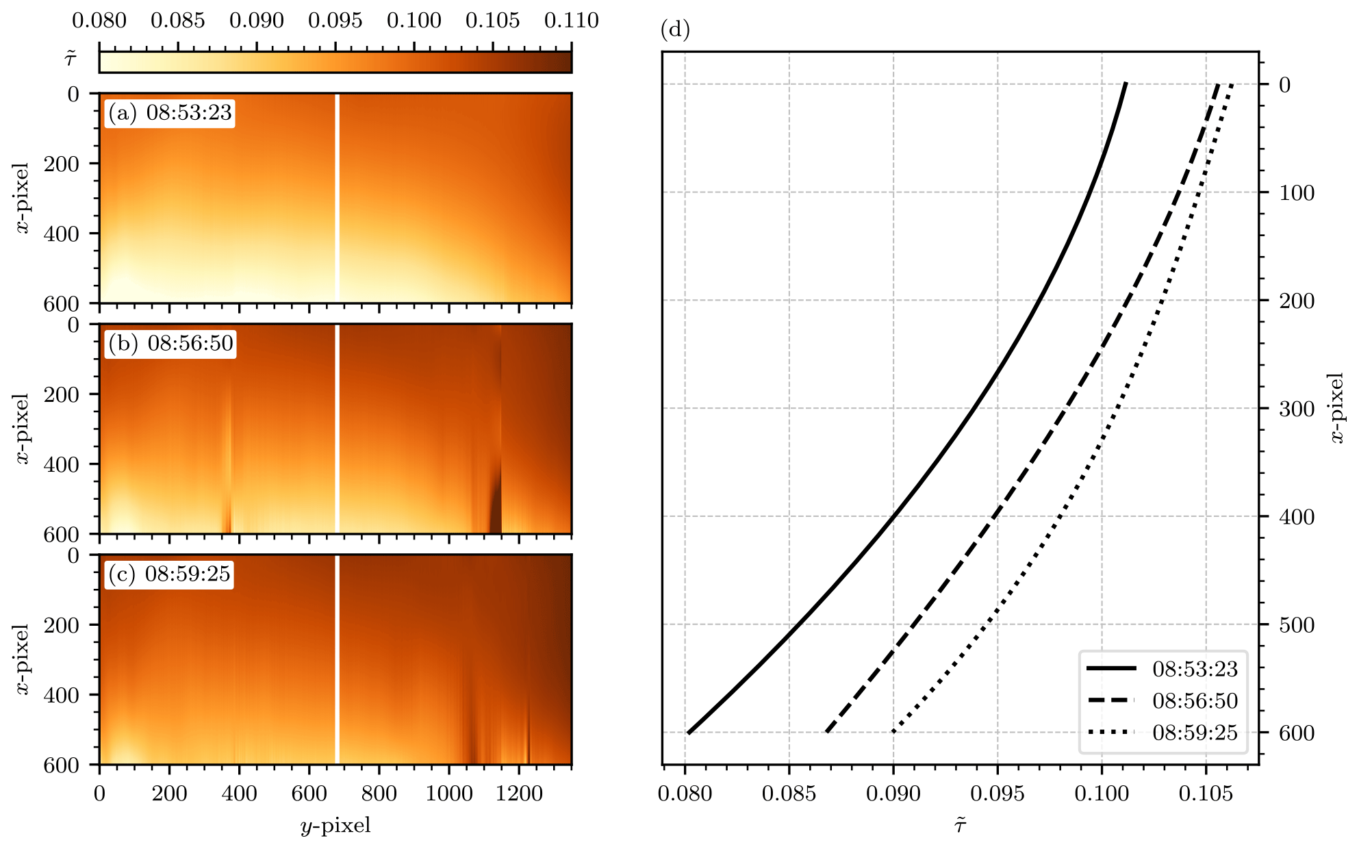
Figure 13 Temporal variance of the background images obtained from the background fit routine described in Sect. 4.2.1. Panels (a)–(c) show the background fit to three images acquired at 08:53:23 UTC+2, 08:56:50 UTC+2, and 08:59:25 UTC+2, respectively. (d) Plots of the background signal along the white vertical lines at y=660 in (a)–(c). Altogether, the figure demonstrates the temporal variability in both magnitude and shape of the background signal.

Secondly, a background image ${\stackrel{\mathrm{̃}}{\mathit{\tau }}}_{\mathrm{background}}$ was subtracted, for which the procedure and reasoning are described in the following. The background image was obtained by fitting a 1D polynomial of degree n to each column of a manually selected set of background pixels, obtained by using a freehand selection tool on the images. This was required because the camera signal images showed large signal gradients across the FOV. We suspect that these gradients are a side effect of the flat-field correction, possibly because the sky, against which the reference images were taken, is generally not radiometrically uniform. An exemplary background correction procedure with n=2 is shown in Fig. 12. The original signal image without background correction, as well as our manual choice of the plume and off-plume regions, is displayed in Fig. 12a. Figure 12b shows the background fit on the basis of that choice. Figure 12c shows the resulting instrument signal image, with a clearly visible plume signal. Figure 12d shows that for an exemplary column at y=660, the background fit tailored very closely to the off-plume region and left a residual in the plume region. Subtraction of the fit made the plume signal visible in the residual, which can be seen in Fig. 12e. A weak temporal dependence of the background image was observed, possibly due to changes in the relative position of the sun (see Fig. 13).

Thirdly, a scalar signal offset ${\stackrel{\mathrm{̃}}{\mathit{\tau }}}_{\mathrm{0}}$ was subtracted. The column density inside the instrument's cell S_c is expected to vary over the course of the measurement. If the two measurement signals J and J_c undergo flat-field correction by the two reference signals J_ref and J_c,ref, unless all signals are recorded with the exact value of S_c, a constant signal offset ${\stackrel{\mathrm{̃}}{\mathit{\tau }}}_{\mathrm{0}}$ will add to $\stackrel{\mathrm{̃}}{\mathit{\tau }}$. For studying time series it is important that this effect is accounted for, i.e., the signal in an off-plume reference region is forced to remain constant, which can be achieved by subtraction of a suitable estimate of ${\stackrel{\mathrm{̃}}{\mathit{\tau }}}_{\mathrm{0}}$. Here, ${\stackrel{\mathrm{̃}}{\mathit{\tau }}}_{\mathrm{0}}$ was computed by averaging the signal $\stackrel{\mathrm{̃}}{\mathit{\tau }}$ over a small rectangle in the off-plume region (the patterned rectangle in Fig. 14) for each image individually.

Finally, the resulting signal images were multiplied with the calibration factor k⁻¹, which was obtained from the instrument model (see Sect. 2.2). This required knowledge of S_c. S_c was therefore estimated according to Eq. (19), considering the same background rectangle as in the calculation of ${\stackrel{\mathrm{̃}}{\mathit{\tau }}}_{\mathrm{0}}$, and a value of $S_{\mathrm{c}}=(\mathrm{2.72}\pm \mathrm{0.04})\cdot {\mathrm{10}}^{\mathrm{18}}$ molec. cm⁻² was obtained. With all corrections included, a single camera image was computed via

$$\begin{array}{}\text{(23)}& S=k^{-\mathrm{1}}\left(S_{\mathrm{c}}\right)\cdot \left(\ln \left({\displaystyle \frac{J_c\cdot J_{\mathrm{ref}}}{J\cdot J_{c,\mathrm{ref}}}}\right)-r-{\stackrel{\mathrm{̃}}{\mathit{\tau }}}_{\mathrm{background}}-{\stackrel{\mathrm{̃}}{\mathit{\tau }}}_{\mathrm{0}}\right),\end{array}$$

where each pixel value S_(i,j) corresponds to the NO₂ slant column density (SCD) measured at pixel (i,j).

4.2.2 Evaluation of an individual camera image

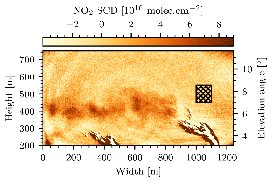
Figure 14 The first image of the measurement. For this image six individual images were averaged, which amounts to 12 s of total exposure. The center of the image shows the positive NO₂ plume signal of approximately 5⋅10¹⁶ molec. cm⁻². The patterned rectangle marks our choice for the off-plume region used to calculate the column density in the gas cell of the instrument S_c, the signal offset ${\stackrel{\mathrm{̃}}{\mathit{\tau }}}_{\mathrm{0}}$, and the detection limit ΔS. At the point of emission (i.e., at a width of 1000 m) the plume was in a fully condensed phase, which, due to optical misalignment of the cameras of the instrument towards the corners of the FOV, generates strong false signals.

Figure 14 shows the first camera image of the series, calculated according to Eq. (23). To obtain this image, the first six consecutive images of the series were averaged. A background fitting routine with polynomial degree n=2 and the same fit mask as displayed in Fig. 12a were used (the choice of this fit mask is discussed further at the end of this section). A positive NO₂ plume signal equalling approximately 5⋅10¹⁶ molec. cm⁻² was observed to be emitted from the chimney of block 7. At the point of emission, i.e., directly above the chimney (at width 1000 m), the plume was in a fully condensed phase and the instrument signal image shows structures of strong negative and positive signal. This effect can be explained as a consequence of the optical setup inside the instrument: the optical axes of the two cameras inside the instrument were adjusted so that there was no displacement of the imaged objects (i.e., the uncondensed part of the plume) in the center of the FOV. However, displacements towards the corners of the FOV could not be avoided. These displacements manifest themselves as strong false signals when the signal ratio of the two cameras is computed. Given that in this measurement they occurred in an image region of low interest, they were deemed unavoidable and not considered any further. In order to obtain the NO₂ SCD and the diameter d of the plume systematically, each column of the NO₂ camera signal image was considered as an individual vertical cross section through the plume. It was observed that the shapes of the measured NO₂ SCDs along these cross sections coarsely followed that of a Gaussian. Figure 15a shows this observation for an exemplary column at y pixel 660. To each image column j, a Gaussian with amplitude A_j, mean μ_j, and standard deviation σ_j was fitted. The NO₂ slant column density and the diameter of the plume at column j were then associated with A_j and 2⋅σ_j, respectively. Columns for which the fit routine did not converge well were ignored. This was considered the case when either the fit failed to converge entirely or the retrieved fit parameters were outside a realistic range ($A_j=S_j>\mathrm{8}\cdot {\mathrm{10}}^{\mathrm{16}}$ molec. cm⁻² or $\mathrm{2}\cdot {\mathit{\sigma }}_j=d_j>\mathrm{100}$ m), which was the case for approximately 50 % of the columns. The resulting NO₂ SCDs and plume diameters are shown in Fig. 15b. The ensemble of all column fits allows for the calculation of an average plume SCD of $S=(\mathrm{4.74}\pm \mathrm{1.21})\cdot {\mathrm{10}}^{\mathrm{16}}$ molec. cm⁻² and an average plume diameter of $d=(\mathrm{78}\pm \mathrm{17})$ m. These values are represented by the red marker in Fig. 15b.

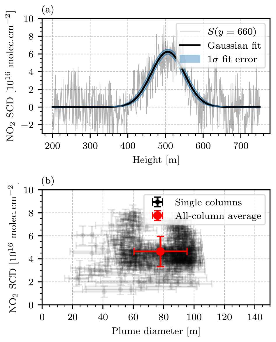
Figure 15 Evaluation of the camera image shown in Fig. 14. (a) Plot of the measured NO₂ column density along the vertical plume cross section along y=660 with a Gaussian fit. (b) Scatter plot of the NO₂ column densities and diameters obtained from the camera image shown in Fig. 14 by fitting a Gaussian to each column of the image. The transparent black scatter points represent the single columns of the image, in which the fit quality criteria described in Sect. 4.2.2 were met. The red scatter point in the center represents the average over all columns.

Figure 16 Comparison of the results from different variants of the background fitting procedure as described in Sect. 4.2.1. Panels (a)–(h) show the procedure for the freehand mask used in Sect. 4.2.1, but with different polynomial degrees of up to n=4. Panels (i)–(p) show the same procedure for a fit mask that covers the entire FOV of the camera images. The results are summarized in Table 2.

Table 2 Summary of results from different variants of the background fitting procedure as described in Sect. 4.2.1 and shown in Fig. 16. The full-FOV fit mask yields smaller plume SCDs and diameters than the freehand mask. n=2, n=3, and n=4 yield similar results for both fit masks.

4.2.3 Uncertainty analysis

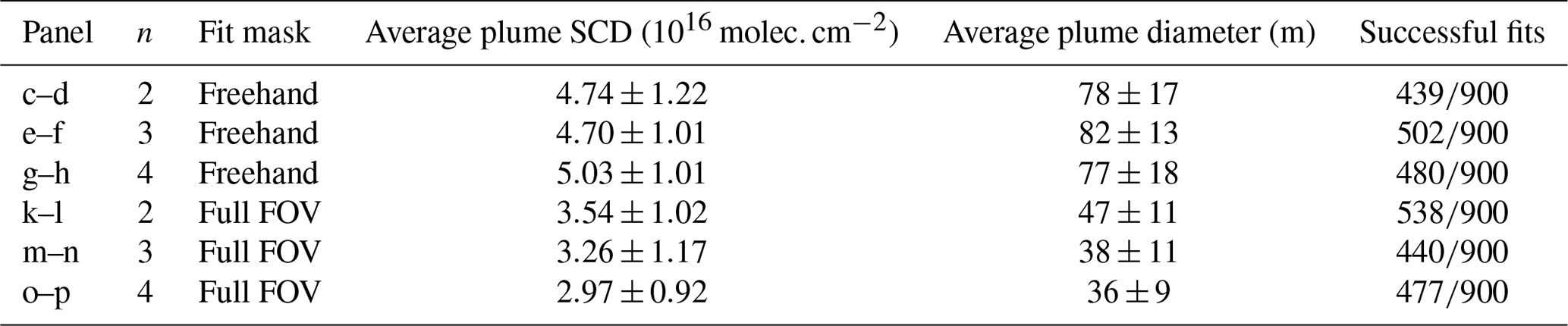
It is necessary to discuss the uncertainties of such an evaluation procedure. It was explained in Sect. 2.2 (see specifically Eq. 17) that the measurement has an intrinsic uncertainty $\mathrm{\Delta }\stackrel{\mathrm{̃}}{\mathit{\tau }}$ of the uncalibrated camera signal due to the Poissonian error of photon counting. This uncertainty propagates directly onto the NO₂ SCDs that are obtained upon calibration of the instrument using k⁻¹(S_c) as described in Eq. (23) and was estimated by computing the standard deviation of the measured NO₂ SCDs in an off-plume region of a camera image, e.g., the patterned rectangle in Fig. 14. A value of $\mathrm{\Delta }S=\mathrm{1.89}\cdot {\mathrm{10}}^{\mathrm{16}}$ molec. cm⁻² was obtained. This is the detection limit of the instrument prototype. In the next step the plume SCDs and diameters were obtained in a Gaussian fit routine for the vertical plume cross sections of all image columns. For a single column j, this introduced additional uncertainties ΔA_j, Δμ_j, and Δσ_j, which were given by the covariances of the fit parameters of that column. These uncertainties propagate into those of the means over all columns, producing the uncertainties used above ($\mathrm{\Delta }S=\mathrm{1.21}\cdot {\mathrm{10}}^{\mathrm{16}}$ molec. cm⁻² and Δd=17 m). Finally, the uncertainties of the background fitting routine as described in Sect. 4.2.1 were investigated. The camera image shown in Fig. 14 was calculated according to Eq. (23), where ${\stackrel{\mathrm{̃}}{\mathit{\tau }}}_{\mathrm{background}}$ was computed using a polynomial of degree n=2 and the same fit mask as displayed in Fig. 12a. Given that this choice of n and the fit mask are subject to our personal assessment, we investigated how much the obtained NO₂ SCD and diameter of the plume vary with different choices of n and the fit mask. Figure 16 shows the results of this analysis. Figure 16a–h show the process of the background fitting routine using the freehand fit mask that was described earlier. Figure 16c, e, and g show the resulting background images ${\stackrel{\mathrm{̃}}{\mathit{\tau }}}_{\mathrm{background}}$ for $n=\mathrm{2},\mathrm{3}$, and 4, respectively. Figure 16d, f, and h show the corresponding scatter plots of NO₂ SCD and plume diameters as obtained from the Gaussian fit routine. Figure 16i–p show the same procedure with a different fit mask, namely one that makes no assumptions of the plume position and covers the entire FOV. The case n=1 was dismissed, seeing that the background signal is clearly not linear (see Figs. 12 and 13). Intercomparison of Fig. 16d, f, and h as well as Fig. 16l, n, and p shows that for a given fit mask the average NO₂ SCD and plume diameter do not vary significantly with the choice of n. Using a full-FOV fit mask yields significantly smaller average values of NO₂ SCD and plume diameter. Furthermore, image objects such as the condensed plumes at y pixels 400 and 1200 lead to vertical fragments in the background image (see Fig. 16j). Overall, the background fitting procedure with n=2 and a freehand selection of the plume as displayed in Fig. 16c and d seems to be a sensible choice because the resulting background image does not suffer from vertical fragments and shows fewer signal variations in the off-plume region. In addition, the fit is fastest to compute for n=2. Table 2 contains a quantitative summary of these findings and allows for the estimation of the uncertainty of the background fitting routine. The uncertainty of the NO₂ SCDs spans from $(\mathrm{2.97}-\mathrm{0.92})\cdot {\mathrm{10}}^{\mathrm{16}}$ molec. cm${}^{-\mathrm{2}}=\mathrm{2.05}\cdot {\mathrm{10}}^{\mathrm{16}}$ molec. cm⁻² to $(\mathrm{5.03}+\mathrm{1.01})\cdot {\mathrm{10}}^{\mathrm{16}}$ molec. cm${}^{-\mathrm{2}}=\mathrm{6.04}\cdot {\mathrm{10}}^{\mathrm{16}}$  molec. cm⁻². The mean is 4.04⋅10¹⁶ molec. cm⁻². Therefore, the overall uncertainty can be estimated as $\mathrm{\Delta }S=\mathrm{2}\cdot {\mathrm{10}}^{\mathrm{16}}$ molec. cm⁻². In analogy an uncertainty of Δd=34 m for the plume diameter is obtained, which will be used throughout the rest of this paper. With this method an estimate of the overall uncertainty of the evaluation is obtained by including not only the statistical uncertainty of the measurement (noisy data), but also the systematic uncertainty that is immanent to the evaluation method. In the future, more elaborate methods for the separation of the plume and background should be investigated. Generally, this would be achieved by image segmentation, for which a variety of methods exists. However, finding an ideal method that generalizes to other plume shapes and viewing geometries would require a study on its own.

A series of camera images was assembled into a video (see Video supplement), which shows the movement of the plume in the wind direction from 08:53 to 09:05 UTC+2.

4.2.4 Optical flow and mass flux analysis

A mass flux analysis was carried out on the basis of image sequences. Given a camera image as shown in Fig. 14, the mass flux through a vertical cross section of the plume can be computed as

$$\begin{array}{}\text{(24)}& F_{\mathrm{m}}={\displaystyle \frac{M_{{\mathrm{NO}}_{\mathrm{2}}}}{N_{\mathrm{A}}}}\cdot v\cdot \int S\left(h\right)\mathrm{d}h,\end{array}$$

where $M_{{\mathrm{NO}}_{\mathrm{2}}}=\mathrm{46.0055}$ g mol⁻¹ is the molar weight of NO₂, $N_{\mathrm{A}}=\mathrm{6.022}\cdot {\mathrm{10}}^{\mathrm{23}}$ mol⁻¹ the Avogadro number, v the wind speed in the horizontal direction, and S the column density, which is integrated along the vertical (height) axis. v was obtained by running a Farnebäck optical flow retrieval (Farnebäck, 2003) on the in-plume region of consecutive camera images. The optical flow was then divided by the time difference Δt between the images. Figure 17a shows the wind speeds associated with the camera image in Fig. 14. For this image and its successor, a mean horizontal wind velocity of $v=(\mathrm{1.48}\pm \mathrm{0.39})$ m s⁻¹ was obtained. The average was considered over the plume region only because in the still background the Farnebäck algorithm cannot detect any flow and returns a wind speed of 0. Similar to the column-wise evaluation of the NO₂ SCD and plume diameter in Sect. 4.2.2, the NO₂ mass flux was computed through each column separately, according to Eq. (24).

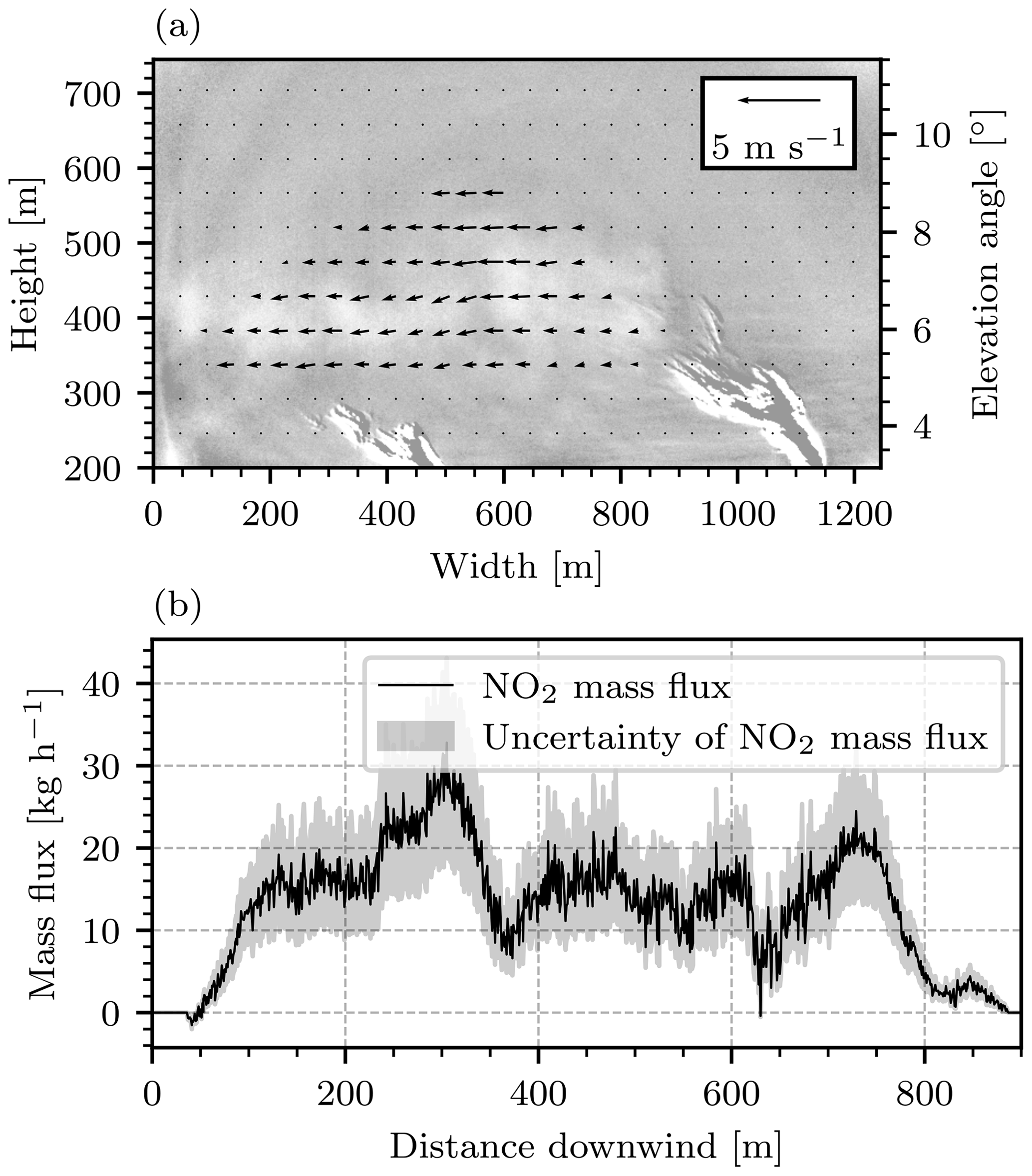
Figure 17 (a) Wind speeds determined from the camera image in Fig. 14 and its successor by application of the Farnebäck algorithm. The wind field is displayed as a vector field in the plume region. (b) NO₂ mass flux obtained from the camera image shown in Fig. 14 and the wind field shown in (a). The mass flux was plotted against the distance downwind, measured from the point at which the fully condensed part of the plume ends (at a width of 840 m in a).

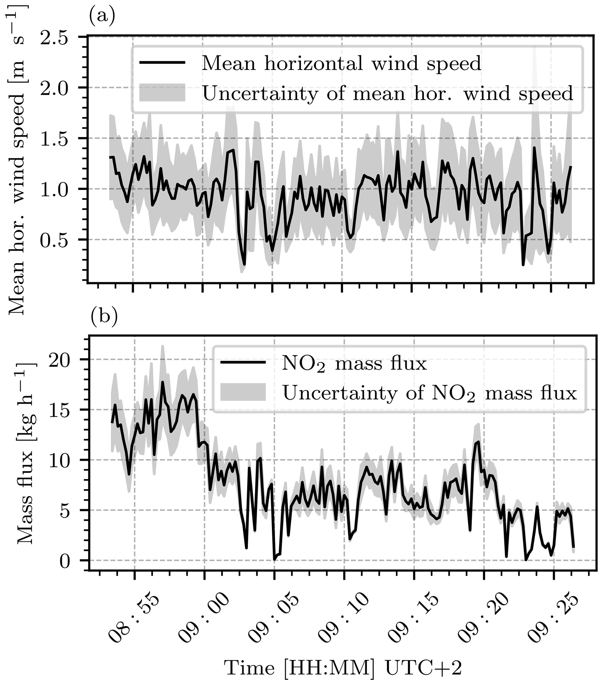
Figure 18 Evaluation of average horizontal wind speeds and NO₂ mass fluxes based on the camera images recorded on 26 April 2021 between 08:55 and 09:25 UTC+2. (a) The mean horizontal wind speed, as obtained from the Farnebäck algorithm for consecutive image pairs. (b) The resulting mean NO₂ mass fluxes calculated according to Eq. (24).

Figure 17b shows the NO₂ mass flux obtained through the individual columns of the image that was displayed in Fig. 14, plotted against the distance traveled downwind from the point at which the fully condensed part of the plume ended (see Fig. 14 or 17a at width 840 m). This procedure yielded a mean mass flux of $F_{\mathrm{m}}=(\mathrm{13.6}\pm \mathrm{7.9})$ kg h⁻¹. The evaluation was extended to obtain average wind speeds and mass fluxes as a function of time. The results are displayed in Fig. 18. Figure 18a shows the mean horizontal wind speed and Fig. 18b shows the mean NO₂ mass flux.

Over the observed time frame from 08:55 to 9:25 UTC+2, an overall mean horizontal wind speed of $v=(\mathrm{0.94}\pm \mathrm{0.33})$ m s⁻¹ and an NO₂ mass flux of $F_{\mathrm{m}}=(\mathrm{7.4}\pm \mathrm{4.2})$ kg h${}^{-\mathrm{1}}=(\mathrm{64.5}\pm \mathrm{36.8})$ t yr⁻¹ were obtained.

A combination of several publicly available sources can be used to estimate a reference value for the NO_x mass flux of the GKM, which can be compared to the value measured here. Of course, the NO₂ camera data only allow computation of the NO₂ mass flux, not the NO_x mass flux. However, the large FOV of the camera covers a total distance of up to 1000 m downwind from the point of emission. It can therefore be expected that the main chemical conversion processes (see Reactions R1–R3) have reached equilibrium and the Leighton relationship is valid. In that case the mass fluxes of NO₂ and NO_x should be of comparable magnitude.

The Fraunhofer Institute for Solar Energy Systems (ISE) reports that the GKM was producing 70.6 MW at 09:00 UTC+2 on the day of measurement (see Fraunhofer Institute for Solar Energy Systems, 2021). The European Pollutant Release and Transfer Register lists an NO_x emission of the GKM of 2890 t yr⁻¹ in 2017 (The European Commision, 2017). The business report of the GKM of the same year states a mean power production of 1119 MW (Großkraftwerk Mannheim Aktiengesellschaft, 2018). Therefore, the GKM should have been running at approximately 6.3 % of its average power. Assuming that the NO_x emission scales linearly with the power produced, an NO_x mass flux of F_m=182 t yr⁻¹ is expected. The mean mass flux obtained from the camera data is significantly lower and amounts only to about one-third of this reference value. Given that the reference is an NO_x mass flux and the NO₂ camera can only detect the NO₂ mass flux, such deviations are expected. The NO₂$/$NO_x ratio of the plume is further investigated in Sect. 4.2.5.

It should be taken into account that this analysis contains two further uncertainties: firstly, although the most recent available data were used, there may be differences in the reference values between 2017 and 2021 (e.g., total mass of yearly emitted NO_x or mean power production). The E-PRTR data show a decline in total yearly emitted NO_x from 2007 to 2017, and it can be expected that this trend has continued until 2021. It should be taken into account that a comparison between a mean flux observed in a time frame of 30 min and a yearly average reference flux is hardly indicative for the accuracy of our measurement. Secondly, GKM block 7, the emitted plume column densities of which were used for this analysis, was not the only active block at the time of the measurement. During the measurement, emissions from GKM blocks 6 and 8 were observed as well, but the FOV of the NO₂ camera was too small to record the plumes emitted from all blocks simultaneously. It is plausible to assume additional emissions of NO₂ from GKM block 6 and 8, which could not be examined on the basis of our measurement.

Although the discussed uncertainties do not allow for a definite conclusion on the overall accuracy of the mass flux analysis, we present the results as a demonstration that flux analyses on the basis of image data with high spatiotemporal resolution are feasible.

4.2.5 Estimation of [NO₂] $/$ [NO_x] ratios

The camera images can be used to investigate the conversion of NO to NO₂ by the reaction of NO with ambient ozone (see Reaction R1) and direct oxidization by molecular oxygen (see Reaction R2). The NO${}_{\mathrm{2}}/{\mathrm{NO}}_x$ ratio can be modeled according to Janssen et al. (1988) by the formula

$$\begin{array}{}\text{(25)}& {\displaystyle \frac{\left[{\mathrm{NO}}_{\mathrm{2}}\right]}{\left[{\mathrm{NO}}_x\right]}}=\left(\mathrm{1}-e^{-ax}\right)\cdot \left({\displaystyle \frac{\left[{\mathrm{O}}_{\mathrm{3}}\right]}{A+\left[{\mathrm{O}}_{\mathrm{3}}\right]}}\right),\end{array}$$

where x is the distance downwind from the point of emission, and [NO₂], [NO_x], and [O₃] denote the concentrations of NO₂, NO_x, and O₃. The model has a parameter $a=k\left[{\mathrm{O}}_{\mathrm{3}}\right]/v$, where k is the rate constant for the $\mathrm{NO}+{\mathrm{O}}_{\mathrm{3}}\to {\mathrm{NO}}_{\mathrm{2}}+{\mathrm{O}}_{\mathrm{2}}$ reaction and v the wind speed, as well as another parameter $A=J/k$, where J is the photodissociation frequency of NO₂. The rate constant k(T) is temperature-dependent. Lippmann et al. (1980) find the empirical relationship

$$\begin{array}{}\text{(26)}& k\left(T\right)=\mathrm{4.3}\cdot {\mathrm{10}}^{-\mathrm{12}}\cdot e^{-\mathrm{1598}\mathrm{K}/T}{\mathrm{cm}}^{\mathrm{3}}\mathrm{molec}{.}^{-\mathrm{1}}{\mathrm{s}}^{-\mathrm{1}}\end{array}$$

with temperature T. The photolysis frequency J is often cited as approximately $J=\mathrm{8}\cdot {\mathrm{10}}^{-\mathrm{3}}{\mathrm{s}}^{-\mathrm{1}}$ in full sunshine (see, e.g., Platt and Kuhn, 2019) but varies strongly with irradiance (Parrish et al., 1983).

Figure 19 shows an approach to compare the camera measurements with the Janssen model. The parameters of the Janssen model are determined by the wind speed v, the ozone concentration [O₃], the photodissociation frequency J, and temperature T. For the wind speed v=0.94 m s⁻¹ was assumed, as obtained from the optical flow procedure in Sect. 4.2.4. The remaining parameters (ozone concentration, photolysis frequency, and temperature) were obtained by fitting the Janssen model to the measured data points. For this, the first 1000 images of the series were averaged (this amounts to a time window from 08:45 to 09:30 UTC+2). Then the vertical integrals of the plume SCD ∫S(h) dh were computed for each individual column, like in the mass flux analysis in Sect. 4.2.4. The concentration ratio $\left[{\mathrm{NO}}_{\mathrm{2}}\right]/\left[{\mathrm{NO}}_x\right]$ associated with each image column was obtained by normalizing this set of integrated SCDs into the interval [0,1]. This is in accordance with the Janssen model, which predicts an initial concentration ratio of 0 with an exponential convergence towards a concentration ratio of ≤1, depending on the model parameters. Figure 19 shows these obtained ratios as black dots plotted against the distance downwind, measured from the point at which the fully condensed part of the plume ended (see Fig. 14 at width 840 m). By running a least-squares fit routine, an ozone mixing ratio of [O₃]=17.5 ppb, a temperature of 13.9 ^∘C, and a photolysis frequency of $J=\mathrm{6.4}\cdot {\mathrm{10}}^{-\mathrm{3}}$ s were obtained. As a reference, the closest ground-based air quality measuring station (Mannheim-Nord, DEBW005) measured an ozone mixing ratio of 26.8 ppb at 09:00 UTC+2 (Landesanstalt für Umwelt Baden-Württemberg, 2021). However, it should be taken into consideration that such ground-based measurements may not yield representative values for 200–500 m of altitude. Moreover, temperatures of up to 17.3 ^∘C were reported in Mannheim for the day of our measurement (Deutscher Wetterdienst, 2021). Parrish et al. (1983) report similar values of J at solar zenith angles of approximately 60^∘, while the solar zenith angle at the beginning of our measurement was 78^∘.

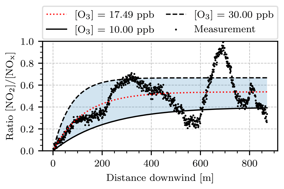
Figure 19 Plot of the $\left[{\mathrm{NO}}_{\mathrm{2}}\right]/\left[{\mathrm{NO}}_x\right]$ ratio as a function of distance traveled downwind, measured from the point at which the fully condensed part of the plume ended (at a width of 840 m in Fig. 14). The black scatter points represent the concentration ratio obtained on the basis of the camera data. The black solid and dashed lines show predictions of the Janssen model for different ozone mixing ratios and a wind speed of v=0.94 m s⁻¹. The dotted red line is a fit of the Janssen model to the measured data points.

Overall, the data points in Fig. 19 coarsely resemble the shape of the Janssen model. However, they oscillate around the prediction of the best fit (red dotted line in Fig. 19). The cause of these oscillations is possibly the alignment of the optical axes of the cameras inside the instrument. It was explained earlier that the camera axes were aligned so that no shifts occur in the center of the FOV due to the displacement of the two cameras. However, shifts towards the corners of the FOV are then inevitable. It was observed that such shifts typically lead to patterns of consecutively increased and decreased false signal in the signal ratio image. The plateau after 400 m of downwind distance agrees with Janssen models assuming ozone mixing ratios of 15–30 ppb. Although such mixing ratios are relatively low for typical polluted urban areas, they are within a realistic order of magnitude. It should be taken into consideration that more recent studies have found initial ${\mathrm{NO}}_{\mathrm{2}}/{\mathrm{NO}}_x$ concentration ratios of 5 %–10 % to be more realistic for the emission from most combustion processes (see, e.g., Kenty et al., 2007, and Carslaw, 2005). This is neglected by the Janssen model, which predicts an initial ${\mathrm{NO}}_{\mathrm{2}}/{\mathrm{NO}}_x$ ratio of zero. Furthermore, as discussed in Sect. 4.2.2, the NO₂ camera is incapable of measuring the NO₂ SCD of the plume directly after its emission when it is still in a fully condensed phase (see Fig. 14). Figure 19 shows the concentration ratio against the distance downwind, which is measured from the point at which the fully condensed part of the plume ended (at a width of 840 m in Fig. 14). The evaluation shown here neglects the plume chemistry of this early phase. To conclude, a crucial uncertainty is the mapping of the column-wise vertical SCD integrals onto the interval [0,1] on both ends: at the lower end, near the point of emission, the concentration ratio is unmeasurable due to the phase of the plume. At the upper end, far downwind, the mapping could be slightly off due to the oscillations of the measured data points. However, we notice good agreement between the obtained fit parameters and the reasonably picked reference values listed earlier in this section.

5 Conclusions

We present a prototype of a novel NO₂ imaging instrument based on gas correlation spectroscopy: the GCS NO₂ camera. It operates by recording images with two cameras, each with a gas cell (cuvette) in front of it; one is filled with air and the other filled with a high concentration of NO₂. The instrument acquires images at high spatiotemporal resolutions of up to $\mathrm{1}/\mathrm{2}$ FPS and 1920×1200 pixels. The instrument response to a wide range of target column densities, ranging up to 1⋅10¹⁸ molec. cm⁻², has been examined in a numerical instrument model. A linear instrument response has been observed within that range, making the instrument easy to calibrate. An examination of the signal-to-noise ratio has shown that the ideal NO₂ column density in the gas cell of the instrument is approximately 4⋅10¹⁸ molec. cm⁻². Furthermore, under realistic conditions, a detection limit of about 2⋅10¹⁶ molec. cm⁻² is expected, which was later confirmed using the instrument prototype. In its current form the instrument is easily transportable and highly cost-efficient with a build price of less than EUR 2000.

A study on the cross-sensitivity to trace gases other than NO₂ was carried out for water vapor and O₄. Under the assumption of realistic column densities of these species the magnitude of the cross-sensitivity of the instrument was predicted to be below an instrument signal equalling $-\mathrm{3.2}\cdot {\mathrm{10}}^{\mathrm{16}}$ molec. cm⁻² of NO₂. The predictions of the instrument model were verified in a proof-of-concept laboratory measurement, in which four test cells were filled with different concentrations of NO₂. Then their column densities were measured with a conventional DOAS setup and the NO₂ camera. We noticed agreement between the two instrumental setups within their uncertainties for all test cells and between the camera results and the predictions of the instrument model. The average relative deviation between model prediction and camera result amounted to 18 %.

We present the results of a field measurement at the coal power plant Großkraftwerk Mannheim. The camera measured an average NO₂ plume SCD of $(\mathrm{4.74}\pm \mathrm{2.00})\cdot {\mathrm{10}}^{\mathrm{16}}\mathrm{molec}.{\mathrm{cm}}^{-\mathrm{2}}$ and an average plume diameter of (78±34) m. In order to increase the SNR of this measurement and smooth the plume signal, sequences of six images were averaged, reducing the effective frame rate to $\mathrm{1}/\mathrm{12}$ FPS and the resolution to 1350×600 pixels. By examination of an off-plume area the detection limit of this measurement was estimated to be $\mathrm{\Delta }S=\mathrm{1.89}\cdot {\mathrm{10}}^{\mathrm{16}}$ molec. cm⁻²; however, the uncertainties of the evaluation procedure, mainly the background estimation, increased the overall uncertainty to $\mathrm{\Delta }S=\mathrm{2.00}\cdot {\mathrm{10}}^{\mathrm{16}}$ molec. cm⁻². A mass flux analysis was carried out on the basis of image sequences. For this purpose, the optical flow between pairs of consecutive images was estimated with a Farnebäck algorithm, which yielded average horizontal wind speeds of (0.94±0.33) m s⁻¹ and a resulting mean NO₂ mass flux of (7.4±4.2) kg h⁻¹ ($\widehat{=}(\mathrm{64.5}\pm \mathrm{36.8})$ t yr⁻¹). The camera measurements showed good agreement with predictions of the Janssen model for plume chemistry when computing the $\left[{\mathrm{NO}}_{\mathrm{2}}\right]/\left[{\mathrm{NO}}_x\right]$ ratio as a function of distance downwind.

In the future, the following improvements to the instrument should be implemented: firstly, the optical setup inside the instrument can be further optimized. By including a beam splitter, the light for both sensor arrays could be collected from a mutual lens, thus eliminating the need to correct for differences in the two lenses as a potential error source, especially the cumbersome background fitting routine described in Sect. 4.2.1. Additionally, there are camera modules with much lower read-out time than the ones used in our prototype, increasing the overall photon budget available for measurements. Secondly, the instrument would benefit from thermal stabilization in order to maintain a more stable NO₂ column inside its gas cell. This way, the evaluation procedure would rely less on successfully determining S_c (see Sect. 2.2) and ${\stackrel{\mathrm{̃}}{\mathit{\tau }}}_{\mathrm{0}}$ (see Sect. 4.2.1) from an off-plume region of the camera images. Thirdly, when measuring NO₂ emissions from a strong source as in Sect. 4.2, the evaluation routine could be made significantly less ambiguous by implementing an automated image segmentation algorithm to separate the plume and off-plume regions of the individual images.

Appendix A: Analytic instrument model

Figure A1 Comparison of the true instrument signal $\stackrel{\mathrm{̃}}{\mathit{\tau }}$, as obtained in Sect. 2.1 (solid line), and the analytical approximation in Eq. (A6) (dotted line). The column density in the gas cell is $S_{\mathrm{c}}=\mathrm{4}\cdot {\mathrm{10}}^{\mathrm{18}}$ molec. cm⁻².

The instrument model presented in Sect. 2.2 allows forward modeling of the measuring process with highly resolved radiance spectra and absorption cross sections. However, the integral terms that occur in the instrument response do not allow for a closed-form expression of $\stackrel{\mathrm{̃}}{\mathit{\tau }}$. Starting from Eq. (12), we simplify the expression for the instrument response by assuming a constant radiance spectrum, $L_{\mathrm{0}}(\mathit{\lambda },t)=\mathrm{const}$ and quantum efficiency η(λ)=const. We restrict the model to some spectral range $\mathrm{\Delta }\mathit{\lambda }=[{\mathit{\lambda }}_{\min },{\mathit{\lambda }}_{\max }]$ and define ${\mathit{\lambda }}_{\mathrm{mid}}=({\mathit{\lambda }}_{\max }+{\mathit{\lambda }}_{\min })/\mathrm{2}$. The final assumption is that the cross section of the target gas consists of only two representative absorption strengths, σ_strong and σ_weak. To determine both, we compute the median of σ_NO2 and define σ_weak and σ_strong as the mean absorption strength below and above the median, respectively. The absorption cross section can then be expressed as

$$\begin{array}{}\text{(A1)}& \mathit{\sigma }={\mathit{\sigma }}_{\mathrm{weak}}\cdot {\mathbf{1}}_{[{\mathit{\lambda }}_{\min },{\mathit{\lambda }}_{\mathrm{mid}}]}+{\mathit{\sigma }}_{\mathrm{strong}}\cdot {\mathbf{1}}_{[{\mathit{\lambda }}_{\mathrm{mid}},{\mathit{\lambda }}_{\max }]},\end{array}$$

where 1_I is the indicator function on an interval I. The instrument response $\stackrel{\mathrm{̃}}{\mathit{\tau }}$ then only depends on the integrals of transmission terms $T_S=e^{-\mathit{\sigma }\cdot S}$ of the following form.

$$\begin{array}{}\text{(A2)}& {\displaystyle }\underset{\mathrm{\Delta }\mathit{\lambda }}{\int }{T}_S\mathrm{d}\mathit{\lambda }& {\displaystyle }={\displaystyle \frac{{\mathit{\lambda }}_{\max }-{\mathit{\lambda }}_{\min }}{\mathrm{2}}}\cdot \left(e^{-{\mathit{\sigma }}_{\mathrm{weak}}\cdot S}+e^{-{\mathit{\sigma }}_{\mathrm{strong}}\cdot S}\right)\text{(A3)}& {\displaystyle }& {\displaystyle }={\displaystyle \frac{{\mathit{\lambda }}_{\max }-{\mathit{\lambda }}_{\min }}{\mathrm{2}}}\cdot \left(T_{S,\mathrm{weak}}+T_{S,\mathrm{strong}}\right)\end{array}$$

Equation (12) then takes the following form.

$$\begin{array}{}\text{(A4)}& {\displaystyle }\stackrel{\mathrm{̃}}{\mathit{\tau }}& {\displaystyle }=\ln \left({\displaystyle \frac{J_c\cdot J_{\mathrm{ref}}}{J\cdot J_{c,\mathrm{ref}}}}\right)\text{(A5)}& {\displaystyle }& {\displaystyle }=\ln \left({\displaystyle \frac{{\int }_{\mathrm{\Delta }\mathit{\lambda }}{T}_S\cdot T_{S_{\mathrm{c}}}\mathrm{d}\mathit{\lambda }}{{\int }_{\mathrm{\Delta }\mathit{\lambda }}{T}_S\mathrm{d}\mathit{\lambda }\cdot {\int }_{\mathrm{\Delta }\mathit{\lambda }}{T}_{S_{\mathrm{c}}}\mathrm{d}\mathit{\lambda }}}\right)\text{(A6)}& {\displaystyle }& {\displaystyle }=\ln \left({\displaystyle \frac{\mathrm{2}\cdot \left(T_{S,\mathrm{weak}}\cdot T_{S_{\mathrm{c}},\mathrm{weak}}+T_{S,\mathrm{strong}}\cdot T_{S_{\mathrm{c}},\mathrm{strong}}\right)}{\left(T_{S,\mathrm{weak}}+T_{S,\mathrm{strong}}\right)\cdot \left(T_{S_{\mathrm{c}},\mathrm{weak}}+T_{S_{\mathrm{c}},\mathrm{strong}}\right)}}\right)\end{array}$$

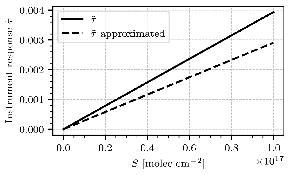
This equation can be applied to arbitrary absorption cross sections; however, σ_weak and σ_strong must be estimated anew for each absorption cross section. The analytical term in Eq. (A6) could be further simplified if a gas without a broadband contribution to its absorption cross section were considered. In that case, σ_weak≈0 and the column in the gas cell S_c could be chosen so that $T_{S_{\mathrm{c}},\mathrm{strong}}\approx \mathrm{0}$. The approximation of the instrument signal would then simplify to

$$\begin{array}{}\text{(A7)}& \stackrel{\mathrm{̃}}{\mathit{\tau }}\approx \ln \left({\displaystyle \frac{\mathrm{2}}{T_{S,\mathrm{strong}}+\mathrm{1}}}\right).\end{array}$$

The true instrument signal $\stackrel{\mathrm{̃}}{\mathit{\tau }}$, as obtained in Sect. 2.1, and the analytical approximation in Eq. (A6) are plotted in Fig. A1. The spectral range of choice was 430–445 nm. The analytical approximation underestimates the true instrument response by around 25 % but is equally linear in S. The deviation can be corrected by tweaking the choice of σ_weak and σ_strong, although good candidates cannot be known a priori. The derived analytical expression allows for quick approximation of the sensitivity of a GCS measurement.