the Creative Commons Attribution 4.0 License.
the Creative Commons Attribution 4.0 License.
 | 16 Mar 2022
Spectral performance analysis of the Aeolus Fabry–Pérot and Fizeau interferometers during the first years of operation
Benjamin Witschas
Christian Lemmerz
Oliver Lux
Uwe Marksteiner
Oliver Reitebuch
Fabian Weiler
Frederic Fabre
Alain Dabas
Thomas Flament
Dorit Huber
Michael Vaughan
In August 2018, the European Space Agency (ESA) launched the first Doppler wind lidar into space, which has since then been providing continuous profiles of the horizontal line-of-sight wind component at a global scale. Aeolus data have been successfully assimilated into several numerical weather prediction (NWP) models and demonstrated a positive impact on the quality of the weather forecasts. To provide valuable input data for NWP models, a detailed characterization of the Aeolus instrumental performance as well as the realization and minimization of systematic error sources is crucial. In this paper, Aeolus interferometer spectral drifts and their potential as systematic error sources for the aerosol and wind products are investigated by means of instrument spectral registration (ISR) measurements that are performed on a weekly basis. During these measurements, the laser frequency is scanned over a range of 11 GHz in steps of 25 MHz and thus spectrally resolves the transmission curves of the Fizeau interferometer and the Fabry–Pérot interferometers (FPIs) used in Aeolus. Mathematical model functions are derived to analyze the measured transmission curves by means of non-linear fit procedures. The obtained fit parameters are used to draw conclusions about the Aeolus instrumental alignment and potentially ongoing drifts. The introduced instrumental functions and analysis tools may also be applied for upcoming missions using similar spectrometers as for instance EarthCARE (ESA), which is based on the Aeolus FPI design.
- Article
(6923 KB) - Full-text XML
- BibTeX
- EndNote


Since 22 August 2018, the first European spaceborne lidar and the first ever spaceborne Doppler wind lidar, Aeolus, developed by the European Space Agency (ESA), has been circling on its sun-synchronous orbit at about 320 km altitude with a repeat cycle of 7 d (ESA, 2008). Aeolus carries a single payload, namely the Atmospheric Laser Doppler Instrument (ALADIN), which provides profiles of the wind component along the instruments' line-of-sight (LOS) direction on a global scale from the ground up to about 30 km (e.g., ESA, 1999; Stoffelen et al., 2005; Reitebuch, 2012; Kanitz et al., 2019; Reitebuch et al., 2020; Straume et al., 2020). With that, the Aeolus mission is primarily aiming to improve numerical weather prediction (NWP) and medium-range weather forecasts (e.g., Weissmann and Cardinali, 2007; Tan et al., 2007; Marseille et al., 2008; Horányi et al., 2015; Rennie et al., 2021). Especially wind profiles acquired over the Southern Hemisphere, the tropics, and the oceans will contribute to closing large gaps in the availability of global wind data, which represented a major deficiency in the global observing system before the launch of Aeolus (Baker et al., 2014). For the use of Aeolus observations in NWP models, a detailed characterization of the data quality as well as the minimization of systematic errors is crucial. Thus, several scientific and technical studies have been performed and published in the meanwhile, addressing the performance of ALADIN and the quality of the Aeolus data products.
Based on airborne wind lidar observations (Lux et al., 2020a; Witschas et al., 2020; Bedka et al., 2021), radiosonde data (Martin et al., 2021; Baars et al., 2020), and wind profiler measurements (Guo et al., 2021), the systematic and random errors in the Aeolus L2B wind product have been analyzed and characterized for different time periods and different geolocations. These studies verified that depending on the respective period of the mission, the respective orbit direction (ascending or descending), the respective Aeolus data processor, and the respective spatial difference between Aeolus observation and reference measurement, the L2B Rayleigh-clear and Mie-cloudy winds show biases of up to several meters per second. To overcome and solve this problem, the identification and correction of systematic error sources were required. Weiler et al. (2021a) for instance demonstrated that the signal detectors of Aeolus have single pixels that show anomalies regarding their dark current signal, which can lead to wind speed errors of up to 30 m s−1 for several hours directly after their appearance, depending on the strength of the atmospheric signal. After implementing a new measurement procedure to characterize the dark current signal and a corresponding correction scheme based on these data, the impact of these hot pixels could remarkably be reduced. The corresponding correction scheme has been operational in the Aeolus L1B processor since 14 June 2019. Furthermore, Rennie and Isaksen (2020), Rennie et al. (2021), and Weiler et al. (2021b) revealed that small temperature fluctuations across the 1.5 m diameter primary mirror of the Aeolus telescope cause varying wind biases along the orbit of up to 8 m s−1. The impact of these thermal fluctuations is successfully corrected by means of ECMWF (European Centre for Medium-Range Weather Forecasts) model-equivalent winds. The correction scheme has been operational in the Aeolus processor since 20 April 2020. After having corrected these systematic errors, a positive impact of Aeolus data in observing system experiments (OSEs) could be demonstrated by Rennie and Isaksen (2020) and Rennie et al. (2021) from the ground up to about 35 km altitude, whereas the largest impact is found in the tropical upper troposphere. Hence, it can be seen that the identification and correction of systematic error sources are mandatory to provide reliable and accurate wind data.
In this paper, Aeolus interferometer spectral drifts and thus potential sources for systematic errors in the wind data product are investigated by means of instrument spectral registration (ISR) measurements that are performed on a weekly basis. During an ISR measurement, the laser frequency is scanned over a range of 11 GHz and thereby resolves the entire free spectral range (FSR) of the double-edge Fabry–Pérot interferometers (FPIs) as well as five FSRs of the Fizeau interferometer. The results of ISR measurements are usually used to perform a so-called Rayleigh–Brillouin correction (RBC) within the Aeolus L2B processor, which takes the different atmospheric temperature and pressure values at different altitudes and geolocations into account to prevent systematic errors in the retrieved winds (Dabas et al., 2008; Dabas and Huber, 2017; Rennie et al., 2020). Additionally, by a detailed analysis of the acquired interferometer transmission curves, conclusions regarding the instrumental alignment and ongoing drifts can be drawn. To do so, respective mathematical model functions are derived and used in non-linear fit procedures. The tools used in this study were developed already before the launch of Aeolus based on measurements performed with the ALADIN airborne demonstrator (A2D) (Reitebuch et al., 2009) and have been adapted accordingly. A first detailed characterization of the A2D spectrometer transmission curves is given by Witschas et al. (2012), a study where the A2D was used to prove the effect of spontaneous Rayleigh–Brillouin scattering in the atmosphere for the first time. Later, the precise characterization of the FPI transmission curves as well as the application of accurate Rayleigh–Brillouin line shape models (Witschas, 2011a, b) allowed atmospheric temperature profiles to be derived from A2D data from the ground up to 15.3 km with systematic deviations smaller than 2.5 K (Witschas et al., 2014, 2021; Xu et al., 2021).
The paper is structured as follows. First, the ALADIN instrument is shortly introduced in Sect. 2, followed by a description of the ISR measurement mode and the data set used in this study (Sect. 3). In Sect. 4, the mathematical tools used to analyze the measured interferometer transmission curves are introduced. Afterwards, in Sect. 5, the time series of respective instrument parameters are shown. In Sect. 6 the presented results are discussed.
An overview sketch of the instrumental architecture of ALADIN is given in Fig. 1. In this paper, the attention is directed to the receiver side of the system. A more detailed description of ALADIN is given in ESA (2008) and Reitebuch et al. (2018); the laser transmitters as well as their frequency stability in space are discussed by Lux et al. (2020a, 2021).
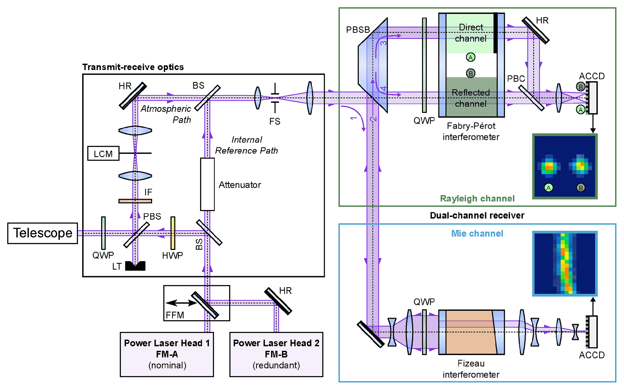
Figure 1Sketch of the ALADIN optical receiver layout reproduced from Lux et al. (2021). QWP: quarter-wave plate; HWP: half-wave plate; PBS: polarizing beam splitter; PBSB: polarizing beam splitter block; PBC: polarizing beam combiner; FFM: flip-flop mechanism; BS: beam splitter; HR: high-reflectance mirror; LCM: laser chopper mechanism; FS: field stop; IF: interference filter; LT: light trap; ACCD: accumulation charge-coupled device.
ALADIN is equipped with two fully redundant laser transmitters, referred to as flight models A (FM-A) and B (FM-B). They are based on frequency-tripled, diode-pumped Nd:YAG laser systems emitting at a wavelength of 354.8 nm (vacuum) and are switchable by means of a flip-flop mechanism (FFM). After passing through a beam splitter (BS), a half-wave plate (HWP) used to define the polarization of the laser light, a polarizing beam splitter (PBS) used to separate transmitted and received light, and a quarter-wave plate (QWP) setting the transmitted laser light to circular polarization, the laser beam is expanded and coupled out by means of a 1.5 m diameter Cassegrain telescope. A small portion of the laser radiation that is leaking through the beam splitter is further attenuated and is used as an internal reference signal, which allows the frequency of the outgoing laser pulses to be monitored as well as measurements of the frequency-dependent transmission curves of the interferometers to be performed as is done, for instance, during ISR measurements (see also Sect. 3). The backscattered radiation from the atmosphere and the ground is collected by the same telescope that is used for emission (mono-static configuration) and is returned to the transmit–receive optics (TRO), where a laser chopper mechanism (LCM) is used to protect the detectors from the signal returned during laser pulse emission after a narrowband interference filter (IF) with a width of about 1 nm has blocked the broadband solar background light spectrum. Furthermore, the transmit–receive optics contain a field stop (FS) with a diameter of about 88 µm to set the field of view (FOV) of the receiver to be only 18 µrad, which is needed to limit the influence of the solar background radiation and the incidence angle on the spectrometers.
Behind the transmit–receive optics, the light is directed to the interferometers that are used to analyze the frequency shift in the backscattered light to finally derive the wind speed along the LOS direction of the laser beam. In particular, the light is first directed to the so-called Mie channel via a polarizing beam splitter block (PBSB). After increasing its diameter to 36 mm by means of a beam expander and with that reducing its divergence to 555 µrad, the light is directed to the Fizeau interferometer, which acts as a narrowband filter with a full width at half maximum (FWHM) of 58 fm (135 MHz) to analyze the frequency shift of the narrowband Mie backscatter from aerosol and cloud particles. The Fizeau interferometer spacer is made of Zerodur to benefit from its low thermal expansion coefficient. It is composed of two reflecting plates separated by 68.5 mm, leading to an FSR of 0.92 fm (2190 MHz), which is chosen to be of the FPI FSR. The plates are tilted by 4.77 µrad with respect to each other, and the space in between is evacuated. The produced interference patterns (fringes) are imaged onto the accumulation charge-coupled device (ACCD) in different pixel columns, whereas different laser frequencies interfere at different lateral positions along the tilted plates. The ACCD does not image the entire spectral range covered by the aperture but only a part of 0.69 fm (1577 MHz), which is called the useful spectral range (USR). This so-called fringe imaging technique using a Fizeau interferometer (McKay, 2002) was especially developed for ALADIN (ESA, 1999).
Table 1Specifications of the Mie spectrometer and the Rayleigh spectrometer of the ALADIN instrument (Reitebuch et al., 2009).
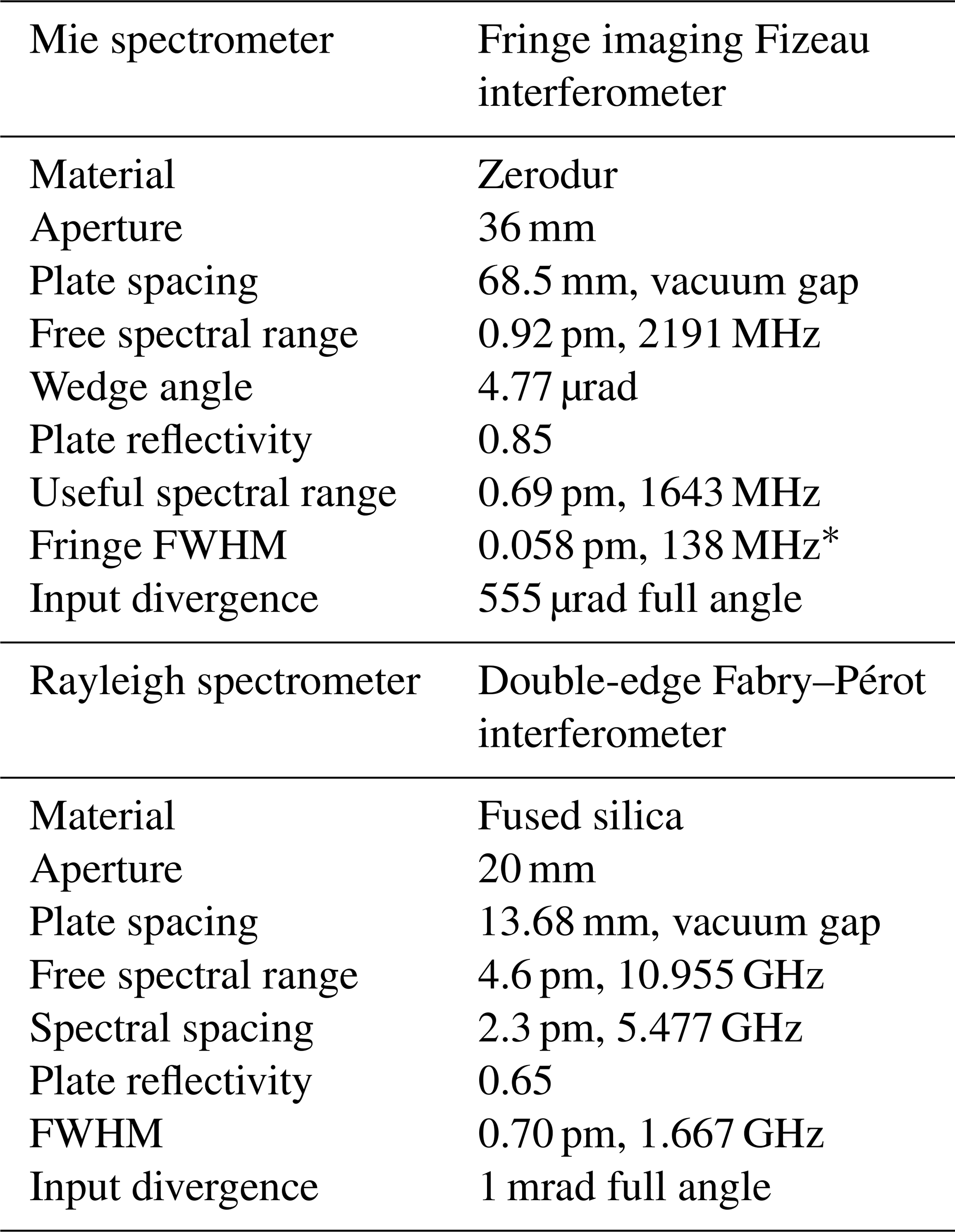
* Not considering a broadening induced by signal accumulation.
The light reflected from the Fizeau interferometer is directed towards the so-called Rayleigh channel on the same beam path and linearly polarized in such a direction that the beam is now transmitted through the PBSB. The Rayleigh channel is based on the double-edge technique (Chanin et al., 1989; Flesia and Korb, 1999; Gentry et al., 2000), where the transmission functions of two FPIs are spectrally placed at the points of the steepest slope on either side of the broadband Rayleigh–Brillouin spectrum originating from molecular backscattered light. For ALADIN, the two FPIs are illuminated sequentially by using the reflection of the first FPI (called direct channel or channel A) to illuminate the second FPI (called reflected channel or channel B). A conceptually similar approach was introduced by Irgang et al. (2002) and was adapted to the double-edge configuration for ALADIN to gain higher radiometric efficiency for the Rayleigh channel. This arrangement also results in different maximum-intensity transmissions for both FPIs compared to a parallel implementation of the double-edge technique with equal filter transmissions. The two FPIs are manufactured by optically contacting the plates to a fused silica spacer with a plate separation of 13.68 mm, leading to an FSR of 4.6 pm (10.95 GHz), whereas the spacing of the direct-channel FPI is further reduced by a deposited step of 88.7 nm (one-quarter of the laser wavelength) to shift its center frequency with respect to the reflected channel by 2.3 pm (5.5 GHz). The space between the plates is evacuated. The plate reflectivity is measured to be 0.65, resulting in an effective FWHM of the transmission curves of 0.70 pm (1.67 GHz), whereas this value does consider defects on the plates as for instance their roughness, bowing, and lack of parallelism. It does not consider any further modifications of the FWHM caused by the spectral characteristics of the light reflected from the Fizeau interferometer. This issue and in general the shape of the interferometer transmission curves are discussed in more detail in Sect. 4.3. The light transmitted through the direct-channel and the reflected-channel FPIs is imaged onto the same ACCD by a single lens after it was combined by an PBC with a small offset angle to 45∘, resulting in two horizontally separated circular spots. As the FPIs are illuminated with a nearly collimated beam of 1 mrad full angle divergence, only the central zeroth order of the inference pattern is imaged onto the ACCD detector. As the FPIs are rather temperature-sensitive (≈ 455 MHz K−1, which corresponds to ≈ 81 ), they are enclosed in a thermal hood to reach a long-term temperature stability of about ± 10 mK. On the short timescale of a wind observation (12 s), the temperature stability is even better than 3 mK, which translates to wind speed variations of less than 0.2 m s−1. For the sake of completeness, the main specifications of the Fizeau interferometer and the FPIs are listed in Table 1.
The values given above and as listed in Table 1 are the essential design parameters and specifications. The actual spectroscopic performance and resultant operational parameters, as for instance the fringe width and shift, line profiles, and measurement accuracies, are profoundly influenced by a multitude of optical and technical considerations. These include alignment accuracy and stability, uniformity of plate illumination, spurious and parasitic reflections, detector non-linearities, and of course any changes or fluctuations therein on short and long timescales. The subject of this paper is thus the evaluation of the impact of these factors, based on detailed analyses of nearly 3 years of spaceborne data. In particular, data from ISR measurements that are performed on a weekly basis are used.
The ALADIN instrument is able to perform special instrument modes that are used for instrument performance monitoring and calibration purposes. One of these modes is the so-called instrument spectral registration (ISR), which is used to characterize the Fizeau interferometer and the FPIs transmission curves and with that to monitor the overall ALADIN instrumental alignment. In the following, the ISR measurement procedure as well as the corresponding data processing steps are shortly elaborated.
3.1 Measurement procedure
During an ISR measurement, the laser frequency is scanned over a range of 11 GHz to cover one FSR of the FPIs and with that about five FSRs of the Fizeau interferometer. The data acquired during an ISR measurement contain 147 observations, and each observation itself contains 3 different frequency steps, which are spectrally separated by 25 MHz. Hence, the ISR frequency range is ( GHz. Each observation consists of 30 measurements, and each measurement consists of 20 laser pulses, whereas the data from the last laser pulse are not acquired during the measurement. Thus, an ISR contains the data of = 83 790 laser pulses, and each measurement at a certain frequency step consists of 10 measurements and contains the data of 190 laser pulses. These settings are not necessarily fixed but could be adapted if required.

Figure 2Mean laser pulse energy versus normalized laser frequency derived from ISR measurements for the FM-A period (a) and FM-B period (b).
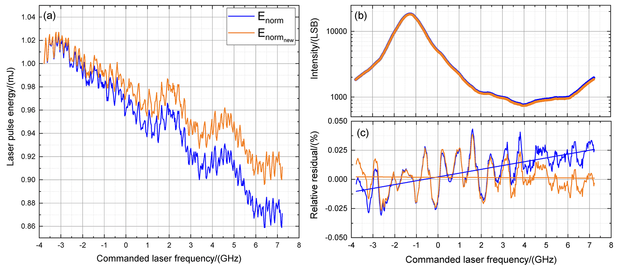
Figure 3(a) Normalized laser energy Enorm(f) (blue) and corrected normalized energy (orange) versus commanded laser frequency for the ISR measurement performed on 10 October 2018 using ξ = 0.04. (b) Corresponding FPI transmission curves of the direct channel according to Eq. (2) by using Enorm(f) (blue dots) and (orange dots) for the laser energy drift correction. To illustrate the small differences, the y axis is plotted with logarithmic scale. (c) Relative residuals of the best fits according to Eq. (9) and line fits.
The raw signal measured within this procedure undergoes several preprocessing steps before being used for further investigations. First, only the internal reference signal is extracted from the data product and analyzed for ISR mode measurements. It is worth adding here that the atmospheric signal is principally available. Internal reference acquisitions with a false pulse validity status or any other corrupt data are eliminated, but no such data were observed for the analyzed ISR data set presented here. The remaining Rayleigh channel signal is then corrected for the detection chain offset (DCO) by subtraction of the mean DCO level, which is implemented to avoid negative values in the digitization, as well as for the laser energy change occurring during the laser frequency scan (see also Figs. 2 and 3). Then, the Rayleigh signal is separated into the one originating form the direct channel (ACCD pixel 1 to 8) and the one from the reflected channel (ACCD pixel 9 to 16). The output data for the Mie channel and the Rayleigh channel are given as the mean intensity per laser pulse according to
where is the total intensity detected per frequency step for the Mie channel or the Rayleigh channel, respectively, and Npulses = 190 is the number of laser pulses during one frequency step (10 measurements). Both quantities, Npulses and , are reported per frequency step in a single so-called AUX-ISR auxiliary file for each ISR Aeolus data product.
3.2 Laser energy drift correction
As the UV output laser energy varies during the frequency scan that is executed during an ISR measurement, the intensity detected per frequency step needs to be corrected accordingly. The trend of the transmitted laser energy is monitored by a photo diode (PD-74) that is mounted in the respective laser transmitter UV section (FM-A and FM-B) behind a highly reflective mirror, an additional diffuser, and neutral-density filters used for further signal attenuation (Lux et al., 2020b). The mean laser energy versus laser frequency derived from the ISR measurements performed between October 2018 and March 2021 is shown in Fig. 2 for the FM-A period (left) and FM-B period (right), respectively. The laser frequency is referenced to the center frequency of the direct-channel FPI transmission curve (see also Fig. 8). Thus, 0 GHz indicates the center frequency of the direct-channel FPI. Brownish colors correspond to the early time of the respective laser period and blueish colors to the later times (see also the label of each panel).
It can be seen that the laser energy changes considerably with frequency for both lasers FM-A and FM-B. For instance, at the beginning of FM-A operation (Fig. 2a, brownish colors), the laser energy was measured to be about 62.5 mJ at lower frequencies (≈ −2.5 GHz) and 53.0 mJ for higher frequencies (≈ 8.5 GHz), which corresponds to a signal decrease of about 15 % during the frequency scan. Furthermore it is obvious that, for FM-A, the laser energy is largest for lower frequencies and decreases with increasing frequency. This is also true for the early FM-B phase until February/March 2020, when a change in the laser cold plate temperature (CPT) caused a spectral shift in the laser energy maximum to be closer to the FPI filter crossing point where also the wind measurements are performed (≈ 2.8 GHz). The laser cold plate couples the laser with the laser radiator, which in turn radiates the heat loss of the laser out to space. Additionally, it can be recognized that the overall laser energy is decreasing throughout the operation time for both lasers, whereas the decrease rate is considerably larger for the FM-A period (Lux et al., 2020b). This circumstance is discussed in more detail in Sect. 5.1. In any case, it is obvious that the Mie and Rayleigh signals obtained during an ISR measurement need to be corrected for the varying laser energy. This is done in the Aeolus L1B processor according to
where is the DCO-corrected raw data as given by Eq. (1), and Enorm(f) is the normalized mean laser pulse energy calculated according to Enorm(f) = , where EPD-74(f) is the signal measured by PD-74 as shown in Fig. 2, and EPD-74(fn=1) is the PD-74-measured energy at the first frequency step. Thus, Enorm(f) does not necessarily range from 0 to 1 as it is normalized arbitrarily to the value of the first data point.
A detailed analysis of the measured FPI transmission curves revealed that the energy correction of the short-wave modulations works reasonably well, but the correction of the overall trend seems to be insufficient. This is especially obvious from the skewness that is visible in the relative residuals of the analyzed FPI transmission curves. Such a tilt is not explainable by incorrectness caused by the fit model as only symmetrical functions are used for the analysis (see also Sect. 4). Thus, it is likely that the energy drift detected by PD-74 is not completely representative of the internal Rayleigh channel signal. Hence, a modified normalized laser energy is needed for a proper energy correction. In particular, it turned out that an additional linear correction according to = leads to satisfying results, with n = 1 to 441 being the number of data points available for ISR measurements, and ξ is a correction factor that is derived by the analysis of FPI transmission curve residuals such that the residual exhibits no skewness anymore. This procedure is illustrated in Fig. 3, where Fig. 3a shows the laser energy measured by PD-74 and normalized to the first data point Enorm(f) (blue) as well as the corrected normalized laser energy (orange) for the ISR measurement performed on 10 October 2018. In Fig. 3b, the respective FPI transmission curves of the direct channel, derived by using Enorm(f) (blue) and (orange) for the laser energy drift correction, are shown. The corresponding relative residuals are shown in Fig. 3c. The line fits applied to the data reveal that the slope is close to zero when is used for the laser energy correction (orange), whereas a significant skewness is obvious when Enorm(f) is used (blue). It can be seen that the relative deviations vary between −2 % and 4 % (peak to peak), whereas the distinct modulation is caused by an insufficient description of the spectral features of the Fizeau reflection and modulations of the incident laser beam profile and/or the transmission over the Fizeau aperture (see also Fig. 5 and the corresponding discussion). For the ISR measurement on 10 October 2018, ξ was determined to be 0.04. For the entire mission time discussed in this paper (October 2018 until March 2021), ξ varies between 0.05 and −0.18. At the beginning of the mission, this energy correction had to be performed manually; however, since December 2018, with the implementation of the L1B processor version 7.05, the additional energy drift correction was added.
Table 2Overview of the ISR data set used in this study.
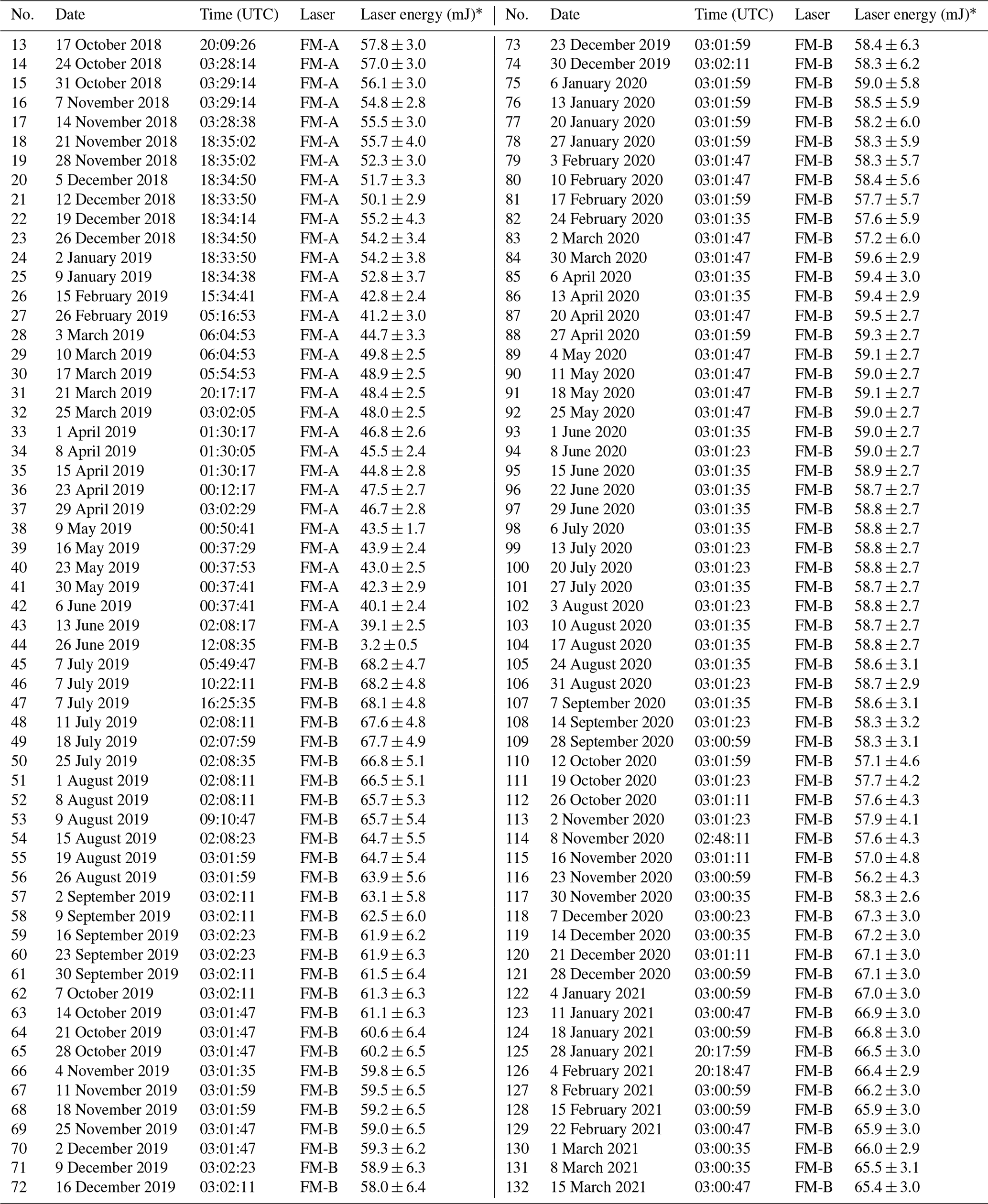
* Mean laser energy and standard deviation per ISR measurement.
3.3 Used data sets
The first ISR measurement in space was performed on 2 September 2018, only 11 d after the satellite launch. The laser was operated at low laser pulse energies of about 11 mJ. On 8 September 2018, the first ISR measurement at full laser pulse reported energy of about 64 mJ was performed to verify the co-registration of the spectrometers. Co-registration means the spectral alignment of the Mie USR center with the FPI filter crossing point. After having changed the Rayleigh spectrometer cover temperature (RCT) and having adjusted the laser frequency accordingly, the first ISR with full laser energy (59 mJ) and co-registered spectrometers was performed on 10 October 2018. This is also the first ISR that is used in this study which ends with the ISR that was performed on 15 March 2021, the last measurement before ALADIN went to survival mode due to an instrument-related anomaly. For the sake of completeness, the date, start time, and mean laser energy of the ISR measurements analyzed in this study are summarized in Table 2.
As explained in Sect. 3, ISR data yield the transmitted signal intensity through the Fizeau interferometer and the FPIs over a frequency range of 11 GHz. These data provide valuable information about the co-registration of the interferometers but also on the overall alignment conditions of the optical receiver as the spectral shape of the interferometer transmission curves depends on various parameters. Such parameters are the interferometer properties themselves (e.g., plate spacing, plate reflectivity, index of refraction of the medium between the plates, plate surface quality), the spectral characteristics of the laser beam (e.g., diameter, divergence, intensity distribution), and the incidence angle of the laser beam onto the interferometers. Thus, the measurement of the interferometer transmission curves and the careful analysis with respective mathematical model functions allow potential changes and drifts of the aforementioned quantities to be investigated. In the following, the model functions for analyzing the interferometer transmission curves are introduced for both the Rayleigh channel (double-edge FPIs) and the Mie channel (Fizeau interferometer).
4.1 Fabry–Pérot interferometers
The particular characteristics of FPIs as well as the corresponding mathematical descriptions are comprehensively summarized in the textbooks by Vaughan (1989) and Hernandez (1986). Another illustrative mathematical description of the characteristics of an FPI that is applied in a direct-detection wind lidar is given by McGill et al. (1997). In this section, the models used to analyze the double-edge FPI transmission curves are demonstrated, and corresponding parameters describing the overall alignment conditions of the ALADIN optical receiver are introduced. It is shown that the sequential arrangement of the interferometers requires some special treatment. Parts of the model functions have already been developed before the launch of Aeolus based on particular measurements performed with the A2D (Witschas, 2011c; Witschas et al., 2012, 2014) and were adapted to ALADIN.
The transmission function 𝒯ideal(M) of an ideal FPI (i.e., axially parallel beam of rays, mirrors perfectly parallel to each other, mirrors of infinite size, and mirrors without any defects) is described by the normalized Airy function according to
where 𝒜 accounts for any absorptive or scattering losses in or on the interferometer plates; R is the mean plate reflectivity; and M is the order of interference which can physically be considered to be the number of half waves between the interferometer plates and which can be written as
where f is the frequency of the transmitted light, n is the index of refraction of the medium between the plates, c is the velocity of light in a vacuum, d is the plate separation, and θ is the incidence angle of the illuminating beam. Furthermore, the frequency change that is needed to change M by 1 is defined as the FSR of the interferometer ℱFSR and is given by
Additionally, the full width at half maximum ΔfFWHM of 𝒯ideal(f) can be calculated according to
where the approximation is valid if the argument of the inverse sine has small values, which is true in the case of R being close to unity.
In reality, however, imperfections and irregularities on the FPI mirror's surfaces cause a change in the intensity transmission of the FPI, which has to be considered when deriving appropriate model functions. Such deviations can for instance be caused by microscopic imperfections on the mirrors, errors in their parallel alignment, or non-uniformities in the reflective coatings which cause the effective mirror separation to vary across the face of the interferometer. As for instance shown by Vaughan (1989), different defect functions can be applied to the Airy function to deal with the various kinds of defects. In the case of ALADIN it turned out that a normally distributed Gaussian defect function according to (Witschas, 2011c)
is well suited for that purpose. Here, σg is the standard deviation of the Gaussian defect function and is called the defect parameter. The convolution of Eqs. (3) and (7) leads to a modified FPI transmission function normalized to unit area according to
where f0 denotes the center frequency. The effect of absorptive or scattering losses is neglected here. In the case of ALADIN, the sequential arrangement of the interferometers also needs to be taken into account (see also Fig. 1), which on the one hand means that the photons within the receiver are recycled but on the other hand means that any spectral imprint of the light reflected from one interferometer is also affecting the spectral characteristics of the transmitted light of the following interferometers. Hence, for the direct-channel FPI, the spectral characteristics of the light reflected from the Fizeau interferometer have to be considered. Accordingly, for the reflected-channel FPI the spectral characteristics of the light reflected from the direct-channel FPI have to be considered. Thus, the spectral shape of the light transmitted through the direct-channel FPI 𝒯dir(f) is described according to
where ℐdir is the mean intensity per FSR, and ℛFiz(f) depicts the reflection on the Fizeau interferometer, which is described by an empirically derived formula according to
where ℐFiz is the modulation depth (peak to peak), is the FSR of the Fizeau interferometer, is the center frequency (valley of the cosine function), and dFiz is the y-axis shift from zero and is set to be constant (dFiz=0.5). Although Eq. (10) is only an approximation of the complex and varying reflection function of the Fizeau interferometer, it provides sufficient accuracy. This is demonstrated in Fig. 4, which shows the normalized Fizeau reflection depending on the commanded laser frequency obtained from the ISR measurement performed on 10 October 2018 (black dots) and the corresponding least-squares best fit using Eq. (10) (light-blue line). In particular, what is contained in the AUX-ISR auxiliary file is the signal transmitted through the Fizeau interferometer depending on the commanded laser frequency 𝒯Fiz(f). Based on that, the reflected signal is calculated without considering any absorption or scattering losses with ℛFiz(f) = 1−𝒯Fiz(f). The overall spectral shape of the Fizeau reflection is well represented by the fit in spectral regions where measurement data are available. In regions where the Mie fringe is out of the USR and not imaged onto the ACCD (e.g., 2.5 to 3.0 GHz), no comparison can be performed.
To describe the transmission through the reflected-channel FPI one additionally has to consider the reflection on the direct-channel FPI and furthermore a potentially leaking beam splitter (see also PBSB in Fig. 1) that could partly lead to a direct illumination of the reflected-channel FPI. Considering that, the transmission through the reflected channel 𝒯ref(f) is described according to
where is the normalized transmission function of the direct-channel FPI. Q takes into account a potentially leaking polarizing beam splitter, allowing for a different from zero, with zero being the value of the ideal case. All other parameters are for the reflected channel as described for the direct channel in Eq. (9).
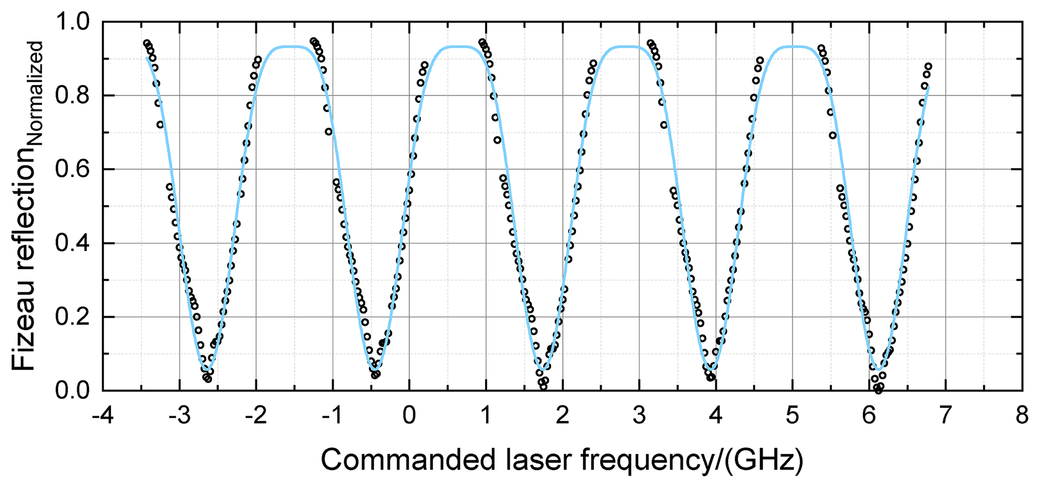
Figure 4Normalized Fizeau reflection depending on commanded laser frequency obtained from an ISR measurement performed on 10 October 2018 (black dots) and the corresponding best fit of Eq. (10) (light-blue line).
To investigate the ALADIN instrumental alignment and ongoing spectral drifts, a fit of Eqs. (9) and (11) to the ISR measurement data is performed by using a downhill simplex optimization method implemented in OriginLab. The sum of the Fourier series describing the Airy function is calculated for 51 terms. Considering a mean plate reflectivity of 0.65, the neglected terms only contribute to about 0.6551 = 3 × 10⁻¹⁰. Except for ℱFSR = 10 946 MHz and dFiz=0.5, all parameters are not constrained and thus a result of the fit routine. The assumption of a constant FSR is justified by the solid arrangement of the FPIs and the temperature stabilization of down to 10 mK, which results in a rather constant plate spacing. Even alignment changes that may alter the incidence angle on the FPI by for instance 5 mrad would change the FSR by only 0.1 MHz.
Based on the determined fit parameters, further quantities that characterize the FPI transmission curves can be derived. The FWHM of an ideal FPI is introduced by Eq. (6). After introducing a defect parameter that takes into account any imperfections and irregularities on the FPI mirror's surfaces, the FWHM can be calculated by describing the convolution of an Airy function and a Gaussian function by a Voigt function whose FWHM can be accurately approximated (Vaughan, 1989; Olivero and Longbothum, 1977). Without considering the reflection on the Fizeau interferometer, the total FWHM () is derived to be
where is given by Eq. (6), and , which accounts for the broadening by defects. Thus, provides a good possibility of monitoring the characteristic FPI transmissions without being influenced by the Fizeau interferometer.
4.2 Fizeau interferometer
In a Fizeau interferometer the plates are set with a wedge angle and spacing chosen to match the spectroscopic problem. The resultant fringes are thus localized at the plates rather than at infinity as in the FPIs. Furthermore, the fringes are straight lines rather than circular and are aligned parallel to the wedge vertex. A textbook analysis of the particular characteristics of the Fizeau interferometer is given by Born and Wolf (1980), drawing on the analyses of Brossel (1947), and has since been expanded upon by many authors (e.g., Kajava et al., 1994; McKay, 2002). These calculations all essentially use classical ray optic techniques and typically show asymmetric fringes, often with appreciable fringe satellites, particularly for larger wedge angles. In this simple ray optic treatment no allowance is made for the local slope of the plates, and no account is taken of diffraction effects.
For the Aeolus Fizeau interferometer the wedge angle is rather small (4.77 µrad), and the plates themselves are subject to “fine grain” surface defects of regular spiral character, due to the magnetorheological optical finishing process. In this situation the resultant fringes can only be modeled by rigorous wave optic techniques (e.g., Jakeman and Ridley, 2006; Vaughan and Ridley, 2013). The resultant wave optic fringe profiles show some asymmetries, but under the Aeolus conditions of operation (small wedge angle and surface defects less than about ± 1 nm) these were shown to be relatively small, and the fringes could be sufficiently described by a Lorentzian function. Hence, for a respective ISR data set, the fringes originating at each frequency step are analyzed by fitting a Lorentzian curve according to
where is the peak amplitude; the FWHM; and x0 the position of the fringe, which is usually called the Mie response. The pixels of the ACCD are numbered from 1 to 16. Thus, when the Fizeau fringe is centered on the ACCD, the center position is halfway between pixel (px) 8 and 9, namely 8.5 px. Hence, each pixel index value from 1 to 16 denotes the center of each ACCD column, resulting in a start value of 0.5 px and an end value of 16.5 px. The fit itself is performed by applying a downhill simplex optimization procedure with Eq. (13). Compared to the FPI analysis, the analysis of the Fizeau fringes is already performed by the Aeolus L1B processor. Thus, , , and the Mie response x0 are available in the AUX-ISR product files.
Furthermore, the Fizeau transmission is calculated at each frequency step as the intensity sum of all 16 px after DCO correction. Additionally, the Fizeau transmission is corrected for the laser energy change occurring during the frequency scan similar to the Rayleigh channel signals (see also Eq. 2); however, an additional energy drift as described in Sect. 3.2 and as is applied for the Rayleigh signal is not considered for the Mie signal. The evaluation of the Fizeau transmission hence gives an approximation of potential changes in the beam intensity profile or beam diameter in one dimension.
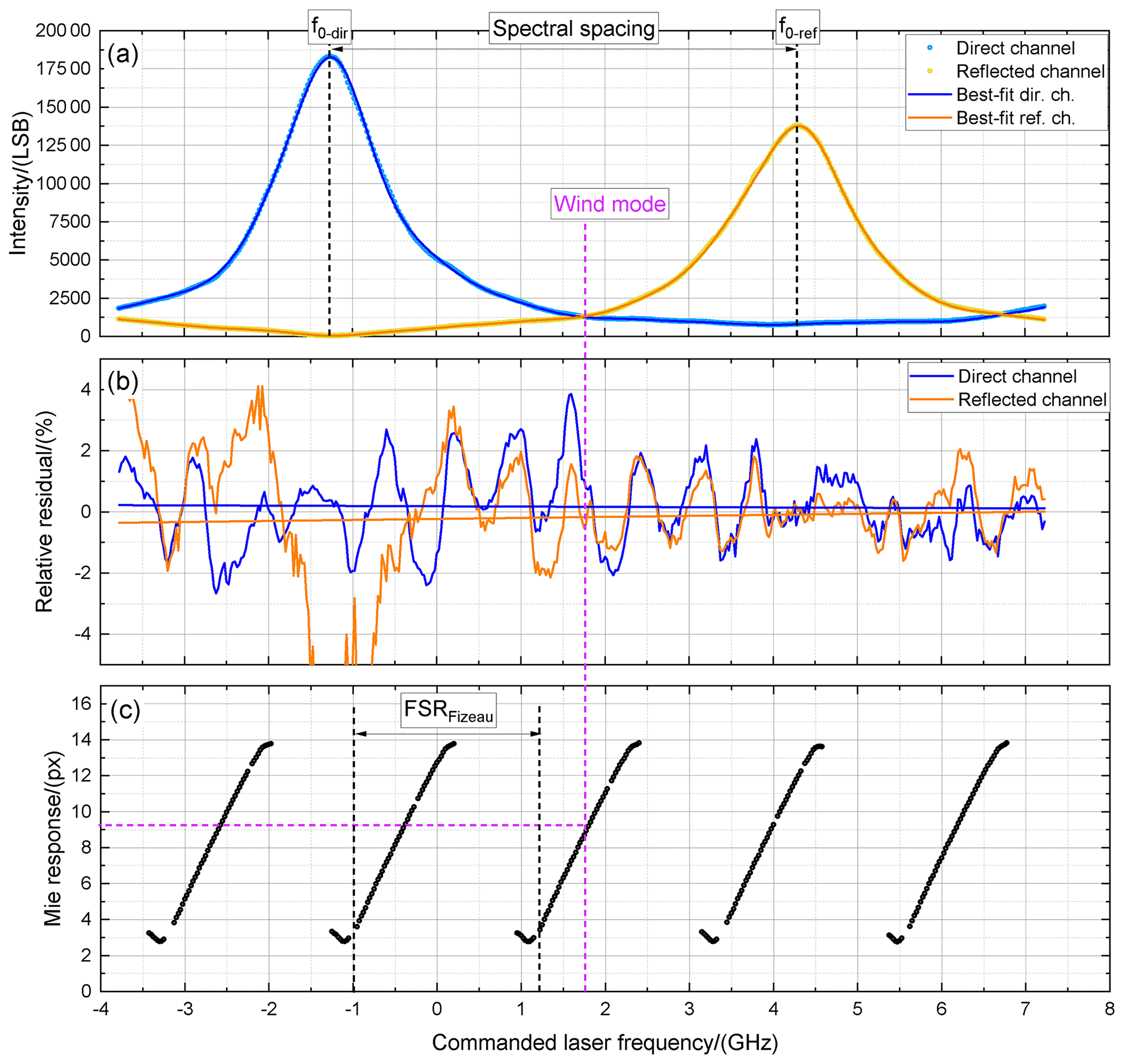
Figure 5(a) FPI transmission curves of the direct channel (light-blue dots) and the reflected channel (yellow dots) measured on 10 October 2018, laser-energy-corrected by means of (see also Eq. 2), and the corresponding best fits according to Eqs. (9) and (11) in blue (direct channel) and orange (reflected channel), respectively. (b) Related relative residuals of the direct channel (blue) and reflected channel (orange). (c) Corresponding Mie response, i.e., the fringe center position on the ACCD pixel.
Table 3Fit parameters according to Eqs. (9), (11), and (12) for energy-corrected ISR data by means of . The given uncertainty in the fit values denotes the standard error derived by the fit routine.
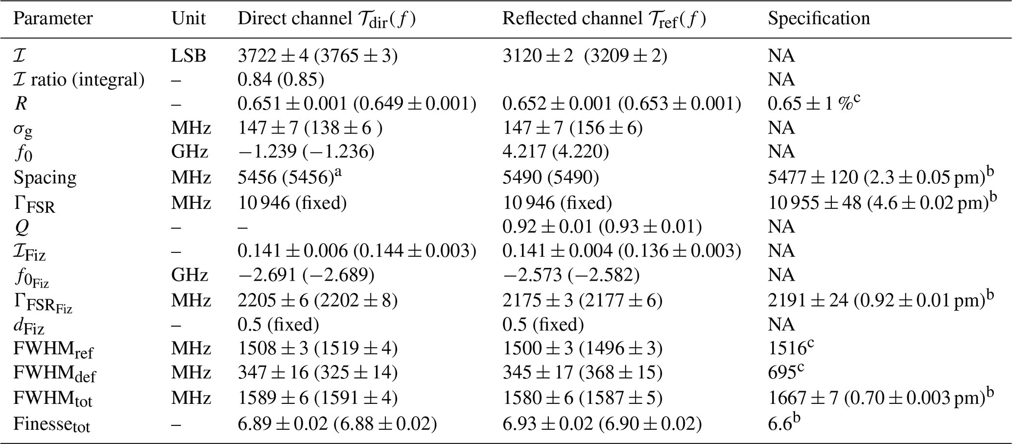
The fit values in brackets denote the one retrieved from the data set corrected with Enorm(f) (see also Sect. 3.2). a Direct channel is at lower frequencies. The second crossing point is calculated by considering the measured FSR. b Values as given by Reitebuch et al. (2009). c Values taken from internal documents of the manufacturer that are not available to the public. NA: no specification available.
4.3 Instrument functions for the Fizeau interferometer and the FPIs on 10 October 2018
The first ISR with full laser energy (59 mJ) and co-registered spectrometers was performed on 10 October 2018. The FPI transmission curves measured on that day including model fits according to Eqs. (9) and (11), the corresponding relative residuals and the derived Mie response are shown in Fig. 5. The corresponding fit results are summarized in Table 3. The given uncertainty in the fit values denotes the standard error derived by the fit routine, and the last column indicates the specification values for comparison.
In Fig. 5a, the measured FPI transmission curve of the direct channel is indicated by light-blue circles and the one of the reflected channel by yellow circles given in least significant bits (LSB), which represent the digitized counts for the photon flux. The transmission curves were laser-energy-corrected by using (see also Eq. 2). The corresponding best fits according to Eqs. (9) and (11) are depicted by the blue and orange lines. Additionally, the frequency used for wind measurements (wind mode) is indicated by the dashed magenta line. The different peak transmission of both FPIs is a result of the sequential arrangement of the interferometers. This circumstance as well as other particular features such as the intensity dip (reflected channel, ≈ −1.2 GHz) and the modulation caused by the reflection on the Fizeau interferometer is adequately represented by the best-fit curves. The mean intensity per FSR is determined by the fit to be 3722 LSB (direct channel) and 3120 LSB (reflected channel), leading to an intensity transmission ratio of 0.84. The respective center frequencies are derived to be −1.239 GHz (direct channel) and 4.217 GHz (reflected channel), leading to a spectral spacing of 5.456 GHz when having the direct channel located at lower frequencies. The corresponding spectral spacing with the reflected channel being located at lower frequencies can be calculated by using the FSR according to 10.946 GHz − 5.456 GHz = 5.490 GHz. Thus, it is almost similar on both sides of the transmission peaks and differs by only 34 MHz. Furthermore it can be seen that the derived spectral spacing on both sides of the filter curves is well within the specification of (5477 ± 120) MHz.
Using the mean plate reflectivity (direct channel: 0.651; reflected channel: 0.652) and the defect parameter (direct channel: 147 MHz; reflected channel: 147 MHz) determined by the fit, of the respective transmission curve can be calculated by means of Eq. (12) to be 1.589 GHz (direct channel) and 1.580 GHz (reflected channel). Thus, the FWHMs of the transmission curves are almost identical when neglecting the imprint of the reflection on the Fizeau interferometer and are smaller than the specified value of (1.667 ± 7) GHz. The numerically determined FWHM from the measured transmission curves however is 1.489 GHz (direct channel) and 1.711 GHz (reflected channel), showing that the Fizeau reflection can change the actual FWHM by several hundred megahertz. Additionally it can be seen that the spectral crossing point of the FPIs is at a commanded frequency of about 1.75 GHz, which is also the frequency used for wind measurements (dashed magenta line).
In the middle panel of Fig. 5b, the relative residual of the direct and the reflected channel as well as linear fits to the data is depicted by the blue and orange line, respectively. The relative deviations vary between −2 % and 4 % (peak to peak), whereas the distinct modulation is caused by an insufficient description of the spectral features of the Fizeau reflection (Eq. 10) and modulations of the incident laser beam profile and/or the transmission over the Fizeau aperture. However, as the Fizeau reflection cannot be measured directly with the instrument being in space, it is difficult to provide a better description without correcting other features that may have a different origin. Still, these features are only a few per cent in amplitude and very constant over time. Thus, the other fit parameters and their temporal trends can be considered to be reliable and not impacted. It is also worth mentioning here that the shown deviations cannot directly be related to a potential systematic error in the retrieved wind speeds as several steps are performed during the wind processing chain. The only processing step that directly applies FPI transmission fit curves is the RBC, which considers the impact of different atmospheric temperatures and pressures on the receiver response (Dabas et al., 2008; Dabas and Huber, 2017). Within the RBC, the FPI fit curves are convolved with Rayleigh–Brillouin spectra of different temperatures and pressures as well as with a tilted top-hat function to consider the different optical illumination between the internal reference path and the atmospheric path. The particular accuracy of the latter procedure cannot be well assessed as there is no possibility of measuring the FPI transmission curves via the atmospheric path with the needed accuracy. Among others, this is the reason why additional bias corrections based on ground return signals or ECMWF model data are performed to obtain a wind product with a small systematic error of below, for example, ≈ 1 ms−1. This bias correction is extensively explained by Weiler et al. (2021b). Additionally, as the width (FWHM) of the Rayleigh–Brillouin spectrum is rather broad (i.e., 3 to 4 GHz for a laser wavelength of 354.8 nm and atmospheric temperatures and pressures), the response of the Rayleigh channel is insensitive to small-scale details as observed for the FPI transmission curve residuals.
As mentioned in Sect. 3.2, the laser energy drift correction may have an impact on the derived FPI transmission curves. Thus, for the sake of completeness, the fit parameters shown in Table 3 are given for both data that were corrected with and for data that were corrected with Enorm(f), given in brackets (see also Sect. 3.2). It can be seen that the energy drift correction has only a minor impact on the retrieved fit parameters and lies within the fit error. Only the obtained mean intensity per FSR shows differences of about 1 % for the direct channel and 3 % for the reflected-channel data.
The Mie response (see also Eq. 13) is shown in Fig. 5c. It can be seen that about five FSRs of 2.2 GHz are measured during an ISR (see also vertical dashed black lines that indicate one FSR). The actual range that can be used for wind measurements (useful spectral range, USR) is represented by the range where the Mie response is almost linear, i.e., about ± 0.6 GHz around each USR center frequency or, for example, the FPI filter crossing point. The Mie USR is usually projected onto the range between pixel column 4 to 14 of the ACCD. The wind measurement is performed at a commanded frequency of 1.75 GHz, resulting in a Mie fringe being located almost in the center of the ACCD detector (pixel 9.2).

Figure 6Normalized FPI transmission curves acquired during ISR measurements performed from 10 October 2018 to 15 March 2021 (see also Table 2) for the FM-A period (October 2018 to June 2019, a) and FM-B period (July 2019 to March 2021, b).
As these kinds of ISR measurements have been performed on a regular weekly basis, they offer the opportunity to analyze time series of the discussed fit parameters and with that to investigate spectral drifts and a change in the alignment conditions of the instrument as discussed in Sect. 5.
In this section, respective fit parameters and their temporal evolution are discussed. These are the detected mean intensity per FSR of the FPIs (Sect. 5.1), the FPI center frequencies and the corresponding spectral spacing (Sect. 5.2), the FPI FWHM (Sect. 5.3), and the Fizeau reflection spectral position (Sect. 5.4). Additionally, the temporal evolution of the Fizeau intensity is analyzed and discussed (Sect. 5.5). All time series show the values retrieved from all ISR measurements performed between 10 October 2018 and 15 March 2021 (see also Table 2).
To first demonstrate the notable alignment stability of the Aeolus optical receiver as well as the reproducibility of ISR measurements, all normalized FPI transmission curves are shown in Fig. 6 for the FM-A period (Fig. 6a) and the FM-B period (Fig. 6b). To be able to directly compare respective measurements, the direct channel transmission curves are normalized to unit area such that = 1, and the reflected channel is normalized accordingly with the same factor as used for the direct channel to keep the ratio between the two respective channels. Furthermore, the x axis is normalized to the direct-channel center frequency and thus marks 0 GHz. Brownish colors correspond to the early time of the respective laser period and blueish colors to the later times (see also the dates shown in the label of each panel).
For the FM-A period, the direct-channel transmission curve is very reproducible. No distinct changes can be recognized except for slight changes originating at a normalized frequency of about −2 GHz, which might be caused by a spectral change in the Fizeau reflection. This is different for the reflected-channel transmission curves. Here, a remarkable drift of both the center frequency and the peak intensity can be observed. As the curves are normalized, this drift is with respect to the direct channel in both the x direction (frequency) and y direction (intensity). Additionally, spectral changes are obvious and probably also caused by changing spectral characteristics of the Fizeau reflection.
For the FM-B period, a center frequency drift between the respective channels is much less or rather not observable. This is also discussed in more detail in Sect. 5.2, which deals with the accurate analysis of the time series of the FPI center frequencies. As for the FM-A period, the peak intensity ratio varies with time. Additionally, it can be recognized that the noise on the transmission curves starts to increase remarkably around August 2020, which is caused by enhanced signal modulations on the internal reference path.
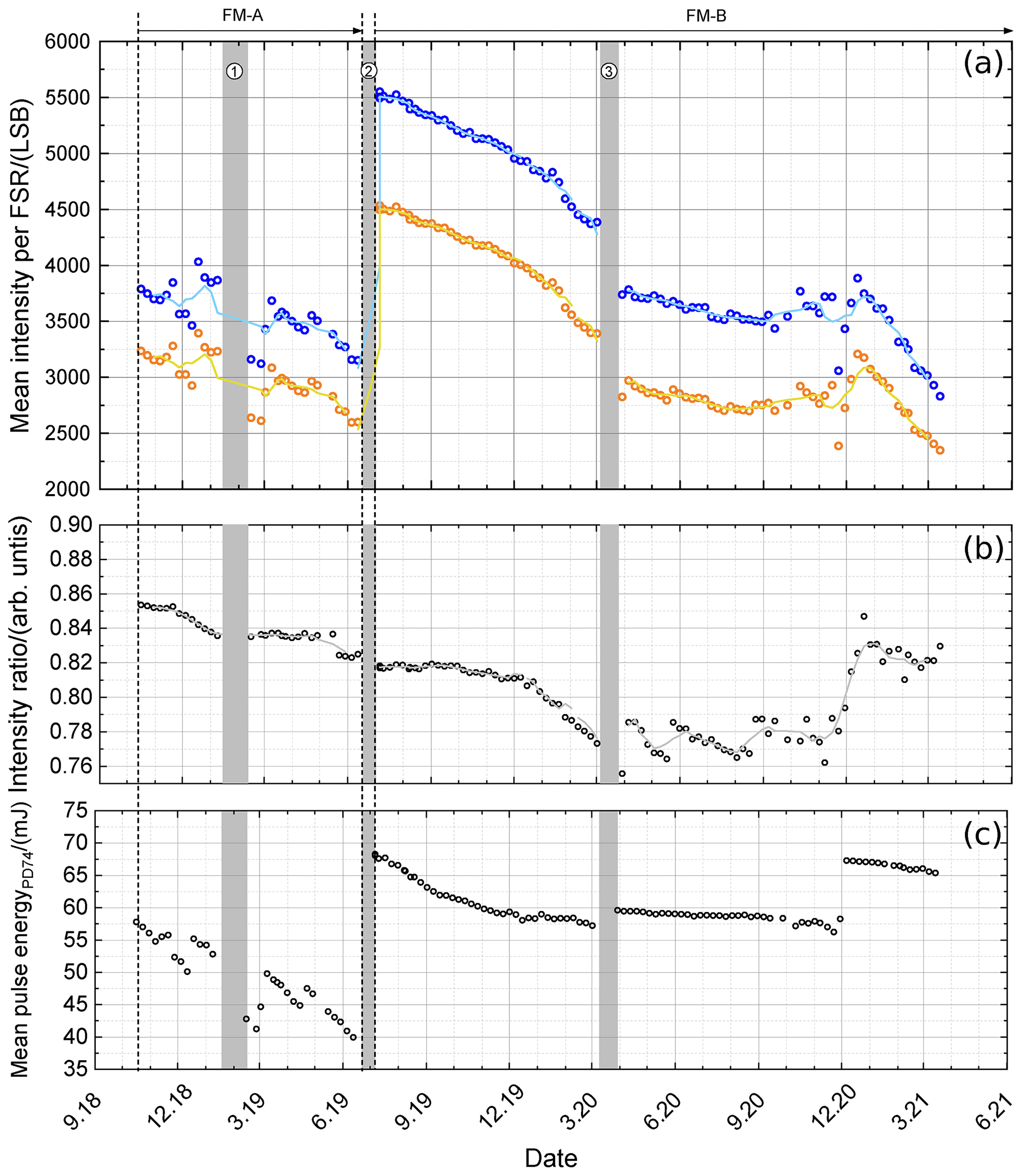
Figure 7(a) Mean intensity per FSR of the direct channel (blue circles) and the reflected channel (orange circles), derived by fitting Eqs. (9) and (11) to the ISR data sets obtained from 10 October 2018 until 15 March 2021 (see also Table 2). The corresponding moving average of five successive data points is indicated by the light-blue line and yellow line, respectively. (b) Intensity ratio (, black circles) and moving average of five successive data points (gray line). (c) Mean laser pulse energy derived from PD-74. Special time periods are indicated by gray bars (1: instrument shut off due to a GPS reboot anomaly; 2: switch from FM-A to FM-B; 3: laser CPT optimization).
5.1 Mean intensity
One quantity that can directly be obtained from the FPI transmission curve analysis by means of Eq. (9) or rather Eq. (11) is the mean transmitted intensity per FSR (ℐdir and ℐref), which provides information about the signal levels on the ACCD detector for the internal reference path. It is worth mentioning that ℐdir and ℐref do not consider the impact of the reflection on the Fizeau interferometer. Thus, the real mean intensity, calculated by integrating the actual transmission curves, would slightly differ from the derived fit values. However, an independent analysis (not shown) has verified that the obtained values are comparable, and the overall trend is similar for the different analyses. The mean intensities per FSR determined for the ISR measurements obtained from 10 October 2018 until 15 March 2021 (see also Table 2) are shown in Fig. 7a for the direct channel (blue circles) and the reflected channel (orange circles), respectively. The corresponding moving averages of five successive data points are indicated by the light-blue line and yellow line. Figure 7b shows the corresponding intensity ratio (, black circles) as well as the moving average of five successive data points (gray line). In Fig. 7c, the mean laser pulse energy during the respective ISR measurements retrieved from PD-74 is plotted. Special time periods as for instance an instrument shut off due to a GPS reboot anomaly (1), the switch from laser FM-A to FM-B (2), and a laser CPT optimization period (3) are indicated by gray bars.
The different periods with the respective lasers FM-A and FM-B can clearly be distinguished as the FM-A laser was operating with about 30 % lower laser pulse energy compared to FM-B (beginning of life), or more precisely, the ACCD detected 30 % less signal on the internal reference path. During the FM-A period, the mean intensity per FSR continuously decreased for both channels except for certain periods that were related to laser parameter optimizations (e.g., pre-amplifier and amplifier current changes in mid-November 2018). The decrease was almost linear in the beginning (October until November 2018 but also later on, from March until June 2019) and is determined to be (−4.7 ± 0.5) LSB d−1 for the direct channel and (−4.4 ± 0.5) LSB d−1 for the reflected channel in the time period from March to June 2019. Considering the initial intensity values of this time period of 3685 LSB (direct channel) and 3084 LSB (reflected channel), this corresponds to a decrease rate of 0.13 % d−1 and 0.14 % d−1, respectively. It is worth mentioning that the analysis of the PD-74 mean laser energy trend in that time period (Fig. 7c) indicates a larger decrease rate of about 0.18 %. This could for instance be explained by alignment changes that led to more photons transmitted through the internal optical path, hence partly compensating the actual laser energy decrease. The intensity ratio (Fig. 7b) changed from about 0.85 to 0.82 during the FM-A period. This change could be due to slightly different alignment changes in the direct-channel and reflected-channel optical paths that influence the transmitted photons differently (e.g., by clipping on other optical elements) and thus change the intensity transmission ratio or due to photons lost outside the ACCD differently for the two channels. It is interesting to realize that the trend of the intensity ratio almost continuously proceeds even when switching from FM-A to FM-B (June 2019), although the overall intensity levels remarkably increase. Furthermore from the bottom panel it can be seen that the overall mean laser pulse energy decreases from about 57.5 mJ in October 2018 to about 40 mJ in June 2019, which corresponds to a decrease of 30 % in the mentioned time period.
Comparing the signal levels at the beginning of the FM-A period (September 2018) and FM-B period (July 2019), an increase of about 37.5 % was achieved (i.e., from 4000 to 5500 LSB for the direct channel). As for the FM-A period, the mean intensity per FSR is continuously decreasing with FM-B. In September 2019, the decrease rate was (−3.7 ± 0.4) LSB d−1 for the direct channel and (−2.6 ± 0.3) LSB d−1 for the reflected channel and thus about 40 % smaller than for the FM-A period. Furthermore it can be seen that the laser CPT change that was performed in March 2020 led to a decrease in the mean intensity levels by about 15 % (i.e., from 4380 to 3740 LSB for the direct channel) but also to a remarkable reduction in the decrease rate, namely to (−1.9 ± 0.1) LSB d−1 for the direct channel and (−1.5 ± 0.2) LSB d−1 for the reflected channel. Interestingly, the mean laser pulse energy (Fig. 7c) increased after the CPT changes, indicating that these changes may have led to alignment changes that induced differences in the signal levels on the internal path, including the Rayleigh ACCD and the PD-74. Since August 2020 the determined fit results from week to week have become more variable due to appearing signal fluctuations in the internal reference signal. At the beginning of December 2020, a laser energy increase of about 15 % was obtained by changing laser operating parameters; however, since mid-December 2020 the decrease rate increased to be (−11.4 ± 0.4) LSB d−1 for the direct channel and (−9.9 ± 0.3) LSB d−1 for the reflected channel. After the laser parameter changes in December 2020, the intensity ratio also changed rapidly (within 4 weeks), from about 0.78 to 0.83, which is another hint that the instrumental alignment changed significantly within this time period. Further indications for ongoing alignment changes can be derived from the time series of the FPI center frequencies, as discussed in the next section.
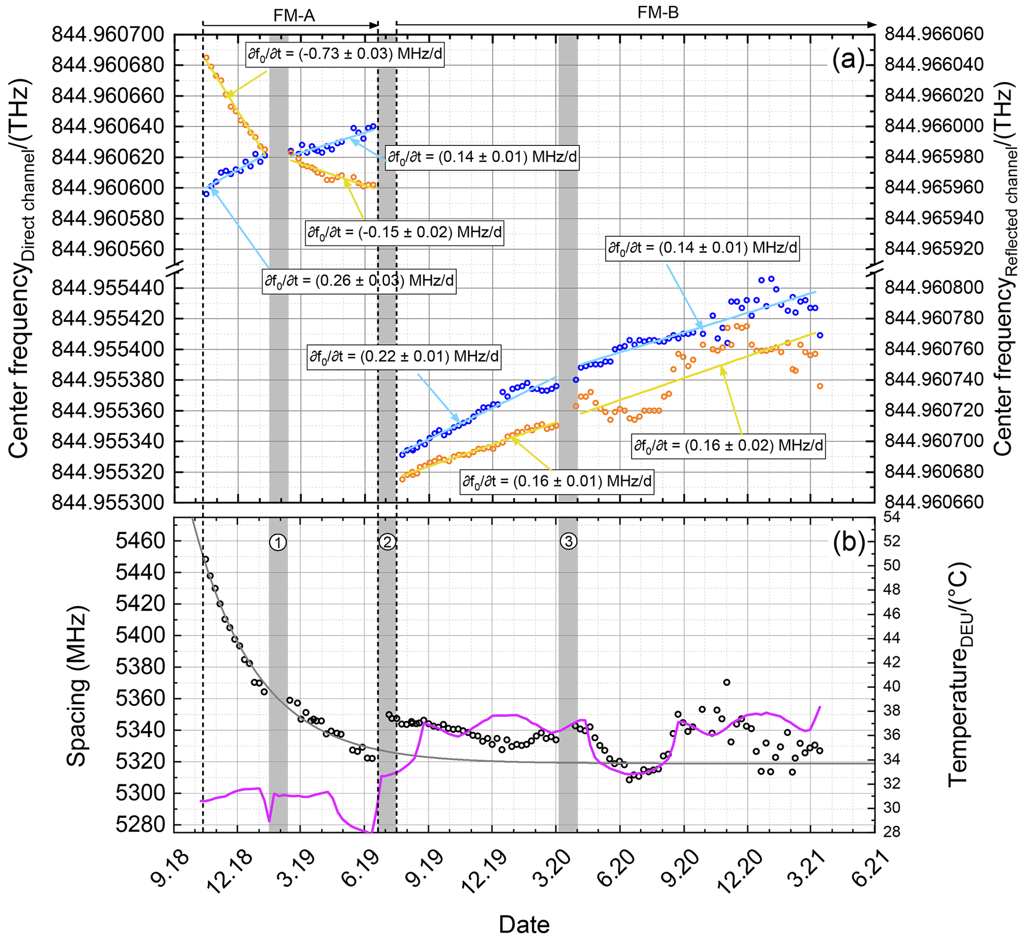
Figure 8(a) Center frequencies for the direct channel (blue) and the reflected channel (orange) derived by fitting Eqs. (9) and (11) to the ISR data sets obtained from October 2018 to March 2021 (see also Table 2). Corresponding line fits to distinct time periods (period 1: 17 October 2018 to 9 January 2019; period 2: 15 February to 13 June 2019; period 3: 25 July 2019 to 2 March 2020; period 4: 30 March 2020 to 15 March 2021) are shown in light blue and yellow, respectively, and the derived slopes () are given by the insets. (b) Corresponding spectral spacing Δf0 between the direct channel and the reflected channel of the FPIs (black circles) and an exponential decay fit (gray) to show the settlement of the spacing drift. Special time periods are indicated by gray bars (1: instrument shut off due to a GPS reboot anomaly; 2: switch from FM-A to FM-B; 3: laser CPT optimization).
5.2 FPI center frequencies and spectral spacing
The center frequencies derived by fitting Eqs. (9) and (11) to the ISR data sets obtained from 10 October 2018 until 15 March 2021 (see also Table 2) are shown in the top panel (a) of Fig. 8 for the direct channel (blue circles) and the reflected channel (orange circles), respectively, whereas the left y axis denotes the direct-channel frequencies and the right y axis the one of the reflected channel. As the derived center frequencies show a larger jump of 5.4 GHz between the FM-A period (September 2018 until June 2019) and the FM-B period (June 2019 until now), the y axes furthermore include a break of the same size. For a better comparability, the frequency range is chosen to be equal for both channels and both the upper and lower part of the panel, namely 150 MHz. Furthermore, line fits to four distinct time periods with almost-linear center frequency drift are shown by light-blue and yellow lines, respectively, whereas period 1 lasts from 17 October 2018 to 9 January 2019, period 2 from 15 February to 13 June 2019, period 3 from 25 July 2019 to 2 March 2020, and period 4 from 30 March 2020 to 15 March 2021. Corresponding slopes of the line fits () are given by the insets. The overall frequency changes for the direct and the reflected channel within the said time periods are 22 and −62 MHz (period 1), 17 and −13 MHz (period 2), 49 and 34 MHz (period 3), and 47 and 53 MHz (period 4). These values are additionally summarized in Table 4. It is worth mentioning that the base laser frequency of 844.961832 THz is not measured but calculated from the laser vacuum wavelength of 354.8 nm that was determined during on-ground tests (Mondin and Bravetti, 2017). The y axis thus shows the commanded laser frequency value plus the laser base frequency. Hence, the 5.4 GHz frequency jump stems from a different absolute frequency of FM-B and could even be a few FPI FSRs different.
Figure 8b shows the spectral spacing between the two FPIs, which is defined as the spectral distance between the center frequencies of the direct channel and the reflected channel according to Δf0 = , where and are the center frequencies of the direct channel and the reflected channel, respectively, and . The spectral spacing for can be calculated according to ℱFSR−Δf0. The gray line indicates an exponential fit to the data set of FM-A (October 2018 to June 2019) to visualize the settlement of the spectral spacing evolution, and the magenta line depicts a temperature time series measured at the ALADIN detection electronic unit (DEU) as it is a good proxy for the ambient temperature within the ALADIN instrument. Special time periods as for instance an instrument shut off due to a GPS reboot anomaly (1), the switch from laser FM-A to FM-B (2), and a laser CPT optimization period (3) are indicated by gray bars.
It can be seen that the center frequencies of both channels are drifting with time by a few megahertz per week throughout the mission. This would not necessarily affect the Aeolus wind retrieval as long as the drift would occur for both channels in the same spectral direction and with the same rate. However, this is not inevitably true in the case of ALADIN. For the FM-A period for instance, it can be recognized that f0 of the respective channels was drifting in different spectral directions and with a different rate. For period 1, the center frequency drift was (0.26 ± 0.03) MHz d−1 for the direct channel and (−0.73 ± 0.03) MHz d−1 for the reflected channel. Thus, the center frequency drift of the reflected channel was about a factor of 2.8 larger and with different sign compared to the one of the direct channel. In the later FM-A phase (period 2) the drift rate settled and equalized to (0.14 ± 0.01) MHz d−1 for the direct channel and (−0.15 ± 0.02) MHz d−1 for the reflected channel, still having a different sign. For FM-B the situation is different. Here, the center frequencies of both channels drift towards the same spectral direction (towards higher frequencies) with a comparable rate. For period 3, the center frequency drift was (0.22 ± 0.01) MHz d−1 (direct channel) and (0.16 ± 0.01) MHz d−1 (reflected channel), whereas for period 4 it was (0.14 ± 0.01) MHz d−1 (direct channel) and (0.16 ± 0.01) MHz d−1 (reflected channel). Thus, the drift rate decreased for the direct channel but stayed constant for the reflected channel. This indicates that the overall alignment conditions or in particular the initial incidence angles for the internal reference path were remarkably different for the different lasers FM-A and FM-B. In Sect. 6, these observations are used to further estimate the underlying reason for these spectral drifts.
Another quantity that can be derived from the center frequencies of both FPIs is the spectral spacing, as shown in Fig. 8b (black circles). The spacing is an important measure as an unconsidered spacing drift would lead to systematic errors in the retrieved wind speeds, whereas an equal center frequency drift with similar rate and spectral drift direction (e.g., as is almost true for the FM-B period) would not affect the wind retrieval. At the beginning of the mission, the spacing is determined to be 5450 MHz and then decreased rapidly to smaller values, which is a result of the center frequency drift occurring towards different spectral directions. Still, the drift of the spacing shows a settlement which is even independent of the switch to the FM-B laser in June 2019. Though the overall spacing changes by about 30 MHz due to the different illumination conditions with the different lasers, the overall settlement of the drift continues. This is also confirmed by an exponential fit (Fig. 8b, gray line) applied to the FM-A data set that indicates an asymptotic convergence at 5320 MHz, which is about the spacing determined for FM-B in early 2021. This finding would lead us to expect that the drifting optical element is not located in the laser transmitters but between the laser transmitter and optical receiver bench, or it would allow for an optical element which is common to the internal path of FM-A and FM-B if not even a rigid-body motion of the laser and/or receiver optical benches with respect to each other.
Furthermore, during the FM-B period, the spacing shows some distinct drift periods as for instance around December 2019 and around June 2020. Comparing these drifts with the ALADIN ambient temperature measured at the DEU of the system (Fig. 8, bottom, magenta line), a correlation (June 2020) and anti-correlation (December 2019 and December 2020) are obvious, whereas the temperature changes are caused by entering or leaving a solar eclipse phase, where parts of the satellite orbit are in darkness, leading to a temperature decrease in the instrument. This finding confirms that the ambient temperature in the system changes and that these temperature changes have an impact on the overall alignment of the instrument even though the temperature of the FPIs only changes by 10 mK during these eclipse periods (not shown).
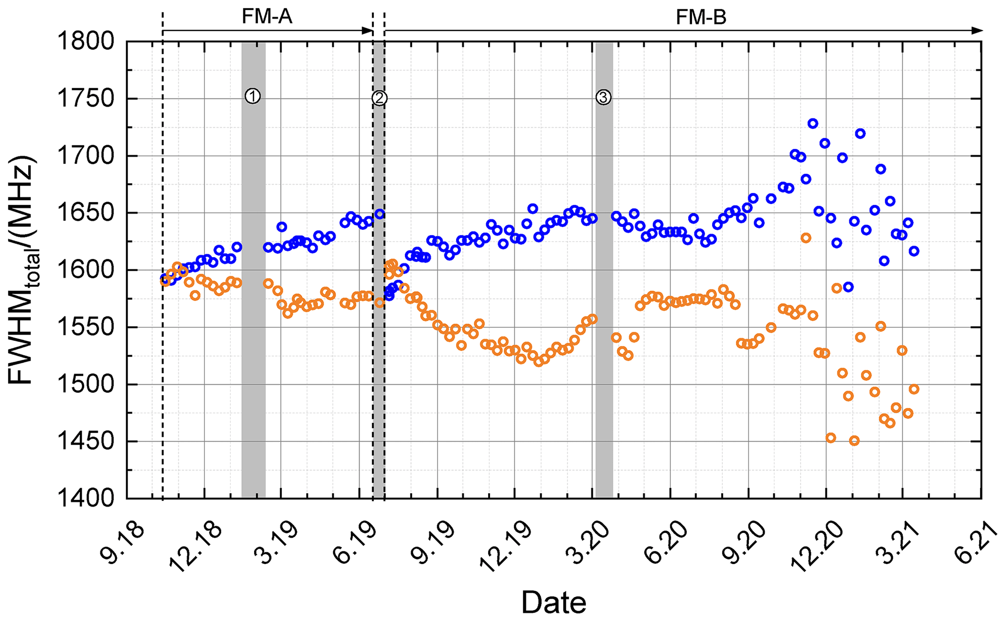
Figure 9Total FWHM of the direct channel (blue circles) and the reflected channel (orange circles), derived by fitting Eqs. (9) and (11) to the ISR data sets obtained from 10 October 2018 until 15 March 2021 (see also Table 2) and calculated according to Eq. (12). Special time periods are indicated by gray bars (1: instrument shut off due to a GPS reboot anomaly; 2: switch from FM-A to FM-B; 3: laser CPT optimization).
5.3 Full width at half maximum
The FWHM of the FPI transmission curves can be calculated according to Eq. (12) using the plate reflectivity and the defect parameter determined by the fit of Eqs. (9) and (11) to the measured FPI transmission curves. The FWHMs for the ISR data sets obtained from 10 October 2018 until 15 March 2021 (see also Table 2) are shown in Fig. 9 for the direct channel (blue circles) and the reflected channel (orange circles), respectively.
It can be seen that the FWHM of both channels was rather similar at the beginning of the mission, namely about 1590 MHz. During the FM-A period, the direct-channel FWHM increased rather constantly by about 60 MHz, whereas it only slightly decreased for the reflected channel, by about 20 MHz. When switching to FM-B, the obtained direct-channel FWHM shows a decrease of about 70 MHz, indicating different alignment conditions for both lasers. Interestingly, the jump is smaller for the reflected channel, namely about 20 MHz. At the beginning of the FM-B phase, the direct-channel FWHM shows an increase from about 1580 MHz to 1650 MHz, where it settles around December 2019. This is the same value that was reached at the end of the FM-A period. On the other hand, the reflected channel shows again a FWHM decrease at the beginning of the FM-B period and seems to settle in May 2020 at a value of about 1570 MHz. Since August 2020 the determined fit results from week to week have become more variable due to appearing intensity variations in the degrading internal reference signal transmission (see also Sect. 6).
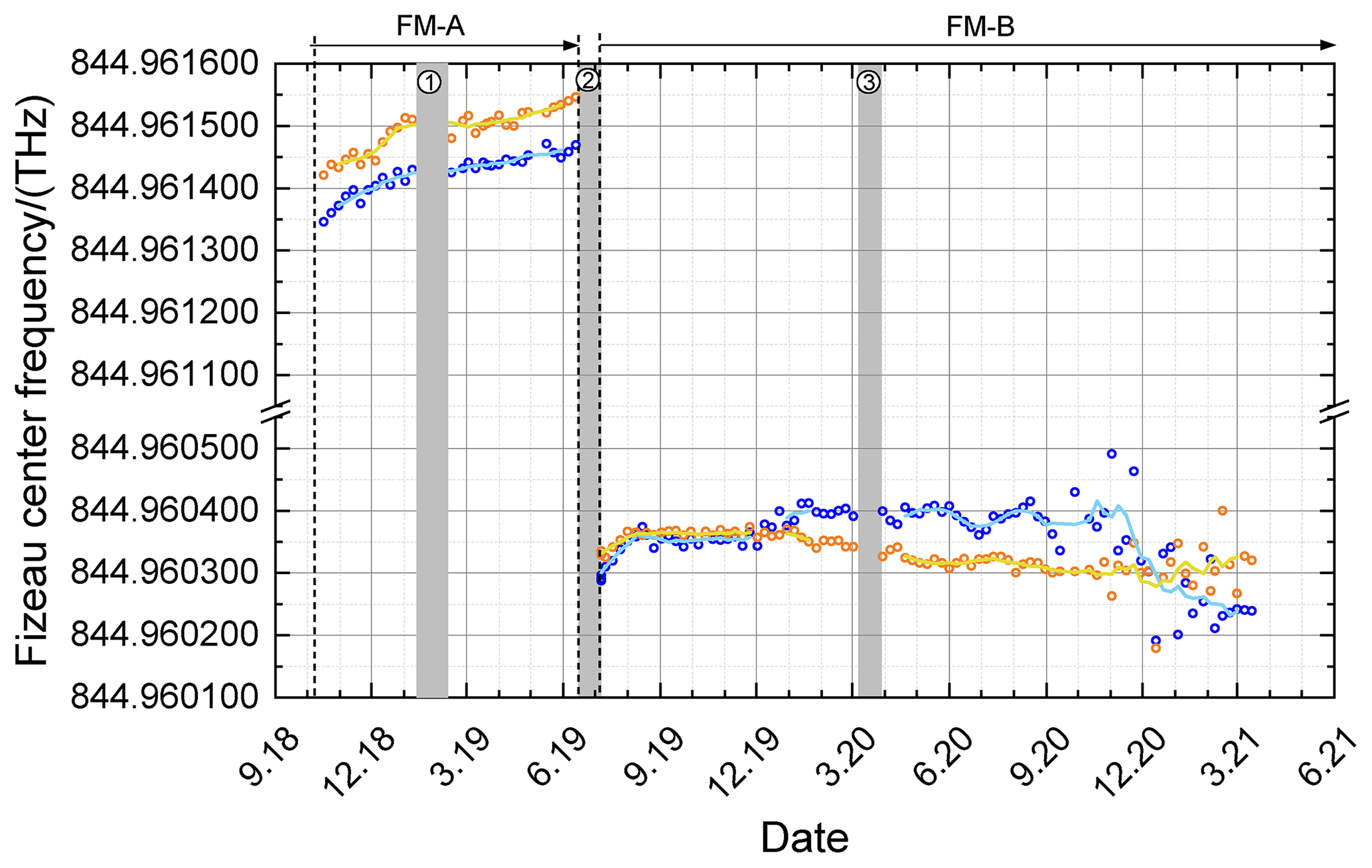
Figure 10Fizeau center frequency derived from the direct channel (blue circles) and the reflected channel (orange circles) by fitting Eqs. (9) and (11) to the ISR data sets obtained from October 2018 to March 2021 (see also Table 2). The corresponding moving average of five successive data points is indicated by the light-blue line and yellow line, respectively. Special time periods are indicated by gray bars (1: instrument shut off due to a GPS reboot anomaly; 2: switch from FM-A to FM-B; 3: laser CPT optimization).
5.4 Fizeau reflection spectral position
The reflection on the Fizeau interferometer has an impact on the FPI transmission curves. Hence, drifts of the spectral characteristics of the Fizeau interferometer reflection can also be derived from FPI analyses. As shown with Eq. (10), the center frequency of the Fizeau reflection is a free fit parameter for the model functions describing the FPI transmission curves. The values determined by fitting Eqs. (9) and (11) to the ISR data sets obtained from October 2018 to March 2021 (see also Table 2) are shown in Fig. 10 for the direct channel (blue circles) and the reflected channel (orange circles), respectively. The corresponding moving averages of five successive data points are indicated by the light-blue line and yellow line. Special time periods as for instance an instrument shut off due to a GPS reboot anomaly (1), the switch from laser FM-A to FM-B (2), and a laser CPT optimization period (3) are indicated by gray bars.
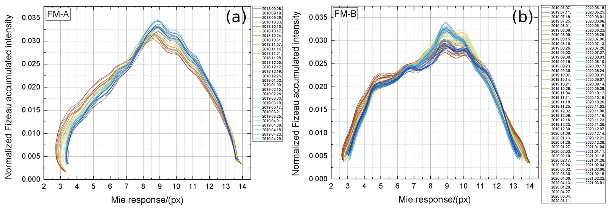
Figure 11Integrated Fizeau intensity versus Mie response obtained during ISR measurements (see also Table 2) normalized to unit area for the FM-A (a) and the FM-B (b).
It can be seen that the Fizeau center frequency is continuously drifting during the FM-A period. In particular, the drift is about 100 MHz within 9 months. Additionally, it can be recognized that the derived trend of the Fizeau center frequency is rather similar for the direct and the reflected channel but has an offset of about 50 MHz, which could be due to the fact that the reflection on the Fizeau is not exactly periodical, and thus, the imprint on 𝒯dir and 𝒯ref is not exactly the same. Nevertheless, it can be concluded that the spectral imprint of the Fizeau reflection on the FPIs is drifting over time during the FM-A period.
During the FM-B period, the situation is different. After switch-on of FM-B, a Fizeau center frequency drift of about 80 MHz was observed until September 2019, followed by an obvious settlement. In December 2019 a drift of about 50 MHz was determined from the direct-channel analysis, whereas the reflected channel showed a drift by a similar amount but in a different spectral direction. This drift is related to a laser CPT jump that occurred on 9 December 2019. The CPT drift that happened afterwards is responsible for the Fizeau center frequency drift. With the settlement of the laser CPT, the derived Fizeau center frequencies also settled until about August 2020. Since then, the obtained fit parameters are in general more variable due to a larger variability in the spectrometer signals, which could be explained by beam clipping happening due to the ongoing alignment drift (see also Figs. 7 and 8). Besides the analyses of the Fizeau reflection impact on the Rayleigh channel signals, Mie channel signals are also available from ISR measurements for further investigations of potentially ongoing spectral drifts. The results of the Mie signal analyses are discussed in the next section.
5.5 Fizeau intensity
The Fizeau intensity is calculated as the sum of the laser energy and DCO-corrected Mie signal at each frequency step and thus gives an approximation of potential changes in the intensity profile or diameter of the beam that is illuminating the Fizeau interferometer (in one dimension). It is worth mentioning that any changes in the measured Fizeau intensity are mainly caused by a variation in the interferometer illumination of the internal path rather than due to a change in the Fizeau transmission itself as the overall illumination is mainly determined by the laser beam profile due to the near-field image of the beam that is used within the fringe imaging technique. The integrated Fizeau transmissions versus Mie response (Eq. 13) obtained during ISR measurements performed from 10 October 2018 until 15 March 2021 (see also Table 2) normalized to unit area (to emphasize the beam shape change) are shown in Fig. 11 for the FM-A period (a) and the FM-B period (b). Brownish colors correspond to the early time of the respective laser period and blueish colors to the later times (see also the label of each panel).
What immediately can be seen is that the Fizeau transmission looks different for FM-A and FM-B and that it evolves with time. Although the pronounced maximum around the Mie response of 9 px is similar for FM-A and FM-B, the distribution for smaller Mie responses looks different, which points to a different intensity distribution of the illuminating beam or rather different illumination conditions as for instance clipping on other optical elements. Additionally, it can be recognized that for both lasers, the width of the Fizeau transmission decreases with time, which could be explained by a shrinking beam diameter or a change in the divergence of the illuminating beam. Furthermore, it is obvious that not only the width but also the overall spectral features are evolving, which might be explained by a changing intensity distribution of the illuminating beam.
In Fig. 8 of Sect. 5.2, the time series of the determined FPI center frequencies was shown and demonstrated different drift behavior for the respective lasers FM-A and FM-B. To understand the observed results and to relate them to respective alignment changes, the equations discussed in Sect. 4.1 have to be revised as they only consider an ideal FPI with mirrors of infinite size, being illuminated normal to the optical axis of the FPI plates by a perfectly collimated beam. In reality however, the illumination cone of the light beam passing through the FPI has a certain FOV with an angular radius θF, also called the input divergence (half of the full cone angle). For the ALADIN internal reference signal is assumed to be µrad, as determined by the parameters of the reference laser beam as it enters the FPI. In contrast, for the atmospheric signal, is estimated to be mrad, as determined by a pinhole aperture in the optical chain. Furthermore, the light beam may illuminate the FPI at a certain angle of incidence θA. Such a situation is illustrated in Fig. 12 for , with 0 denoting the prime optical axis of the system defined as the normal to the FPI plates. Hence, the FPI circular interference fringes (black rings, not shown for the full circle) are centered at 0, but for an off-axis aperture (gray circle) centered at θA only portions of the fringes will be illuminated, as indicated by the orange, light-blue, and dark-blue circular arcs. The dashed lines exemplarily mark the crossing points of the second interference fringe with the aperture or rather the fraction of the second interference fringe that is transmitted through the aperture (light-blue circular arc). The asymmetric behavior of such an off-axis illuminated FPI has been treated in detail by Hernandez (1974) as well as in the textbooks by Hernandez (1986) and Vaughan (1989), whereas only the most important points are recapitulated here. The following analysis is based on the principle demonstrated in Fig. 12.
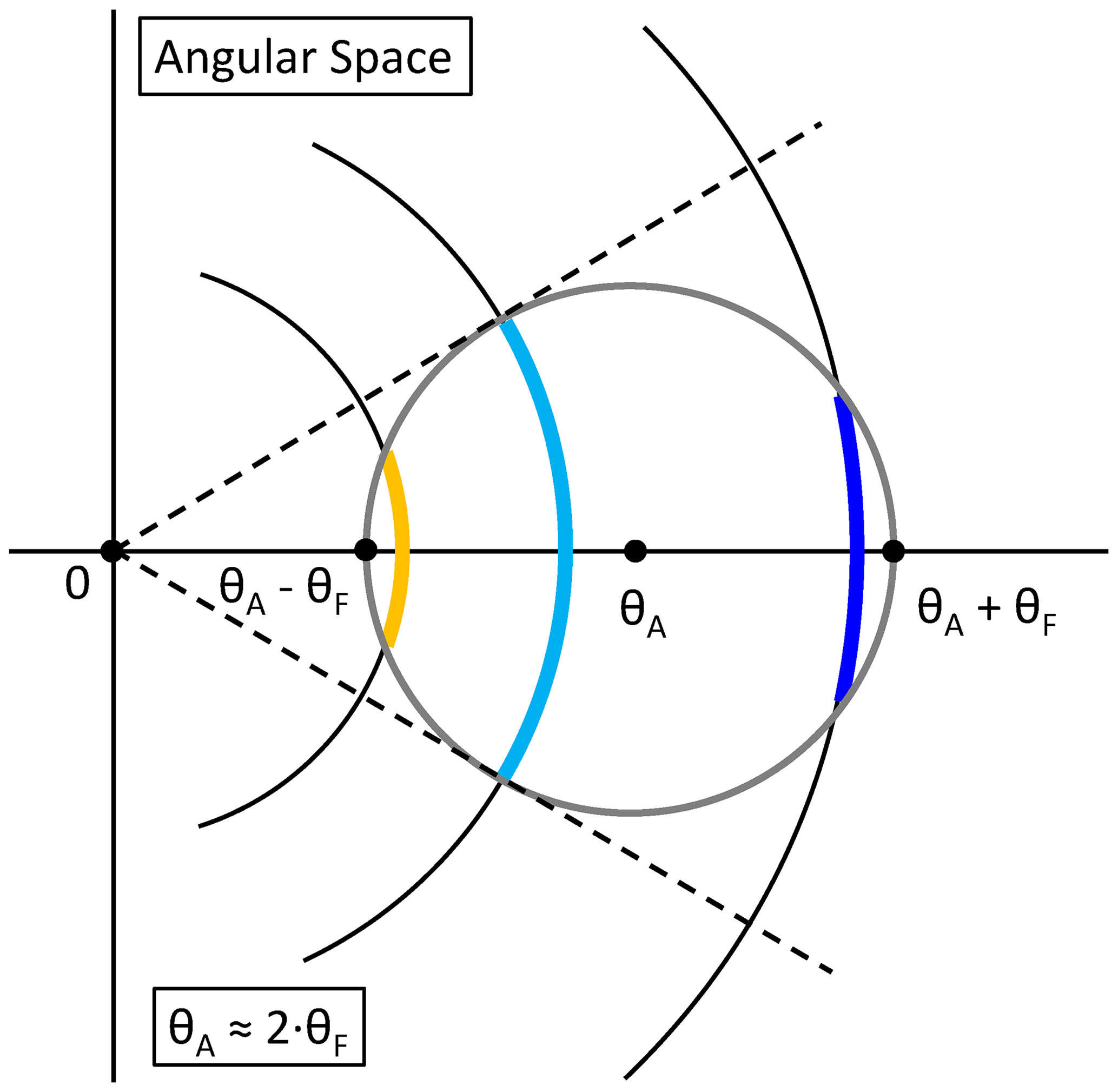
Figure 12Illustration of FPI operation with an angle of incidence θA and a field of view θF in angular space, with 0 denoting the prime optical axis of the system defined as the normal to the FPI plates. The FPI circular interference fringes (black rings) are centered at 0, but only portions of the fringes will be illuminated due to the off-axis centered aperture (gray circle) as indicated by the orange, light-blue, and dark-blue circular arcs. The dashed lines exemplarily mark the crossing points of the second interference fringe with the aperture or rather the fraction of the second interference fringe that is transmitted through the aperture (light-blue circular arc). The detailed analysis leading to Eqs. (14) to (19) and to the dispersion curves shown in Fig. 13 is based on the principle demonstrated here as it is also applicable for the dependence of the zero-order spot imaged on the Aeolus ACCD.
The ideal FPI, as discussed in Sect. 4.1, is an angle-dependent filter with quadratic dispersion. In particular, the transmission for a narrow beam (θF→0) at a certain θA experiences a frequency shift Δf compared to the beam at normal incidence (θA = 0) according to
where θ1 = = 5.093 mrad is the angular radius of the first full fringe and is used as a scaling reference (Vaughan, 1989) as it relates certain angular radii together with ΓFSR to a frequency shift compared to the beam at normal incidence. More precisely, θ1 is the angular radius of the first fringe from the center supposing that a bright fringe of zeroth order exists exactly at the center of the pattern. Hence, the radius of the first full fringe corresponds to one FSR. From Eq. (14) it can also be seen that any change in the angle of incidence would lead to a center frequency increase, as is true for the FM-B period. For ALADIN, λ = 354.8 nm, d = 13.68 mm, and ΓFSR = 10.95 GHz are given according to Table 1. Additionally, by replacing θ1 and ΓFSR with their definitions given above and in Eq. (5), the relative frequency shift compared to the beam at normal incidence is derived to be
For a larger beam with a non-negligible θF, two regions of operation may be considered with θA ≦ θF and θA>θF. For θF>0 and nominal incidence (θA=0), the aperture profile extends out to
and is a top-hat function with a full width Δf0. The median position of this aperture function, which denotes the center of energy, is at half of this value, i.e., , and the peak intensity is usually designated as I0. For 0<θA ≦ θF, the aperture profile starts to become asymmetric and extends out to a full width ΔfW given by
However, the median position of the energy distribution remains constant up to according to . For 0.293 ⋅ θF<θA ≦ θF, the aperture profile becomes increasingly asymmetric with a full width given by Eq. (17). However, the peak intensity remains at I0. The median position θM is given by = so that
where κ≈0.6 to a good approximation. When θA>θF, the incident beam no longer overlaps the optical axis normal to the FPI plates, and the angular position of the peak of the profile is at θp given by = and in frequency terms
and the peak intensity Ip is given by
However the median value which denotes the energy center of the profile is still calculated by Eq. (18) with κ≈0.6.
The corresponding dispersion curves of frequency shift (i.e., median position) versus angle of incidence θA, calculated by means of Eqs. (14) to (20) for beams of different angular aperture θF, are shown in Fig. 13. The green line denotes the ideal case with θF = 0, the red line indicates the case for the internal reference beam with = µrad, and the black line depicts the case for the atmospheric signal beam with = mrad.
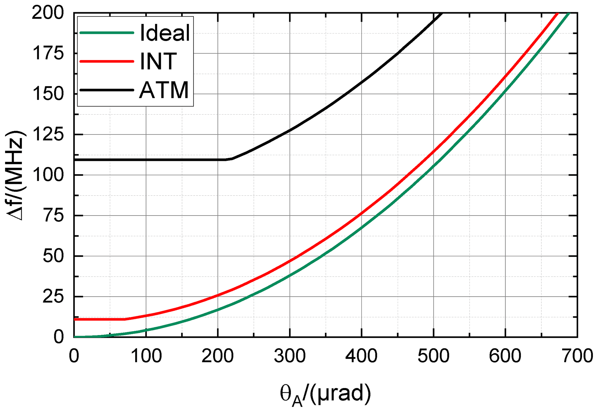
Figure 13Dispersion curves of frequency shift versus angle of incidence for beams of different angular aperture (FOV) with θF = 0 as corresponding to the ideal case (green), = µrad as corresponding to the internal reference beam (red), and = mrad as corresponding to the atmospheric signal beam (black). The frequency shift between internal reference signal and atmospheric signal at nominal incidence is close to 100 MHz.
With Fig. 13 it can be seen that incidence angle drifts of a few hundred microradians are needed to explain the observed center frequency drifts (see also Table 4) for the internal reference beam. It is further obvious that the exact incidence angle drift depends on the initial incidence angle, which is essentially unknown. During the FM-A period, the center frequency drifts by +39 MHz for the direct channel and by −75 MHz for the reflected channel. Thus, as the center frequency decreases for the reflected channel, it can be concluded that the initial incidence angle for the reflected channel was definitely different from normal incidence. For instance, an initial incidence angle of about = 425 µrad and a drift towards normal incidence could explain the observed center frequency drift. For the direct channel, the observed center frequency drift of +39 MHz could be explained by an incidence angle change of about 325 µrad supposing = 0. For = 400 µrad, the incidence angle only has to drift by about 110 µrad to θA = 510 µrad to explain the observed center frequency drifts.
For the FM-B period, the frequency drifts of both channels are comparable and with similar sign. In particular, the center frequency drifts by +96 MHz for the direct channel and by +87 MHz for the reflected channel. Supposing an initial incidence angle of = 0, an incidence angle change of about 475 µrad is needed to explain the observed center frequency drifts. For larger initial incidence angles, the corresponding drift would accordingly be smaller. What can also be recognized during the FM-B period is that the center frequency drift rate for the direct channel decreases over time from () MHz d−1 (period 3) to () MHz d−1 (period 4). As the dispersion curve becomes steeper for larger θA, this behavior can only be explained by a decreasing θA drift rate or a clipping of the beam, which would alter the apparent θF.
Additionally, from Fig. 13 it can be recognized that even for normal incidence (θA = 0), the atmospheric signal is already shifted by about 100 MHz with respect to the internal reference signal, which is due to the considerably larger FOV of the atmospheric signal and which is an important difference between the two signal channels.
Summarized, it can be said that the overall alignment conditions were significantly different for the FM-A and FM-B period. Furthermore, it has to be pointed out that a θA drift of several hundred microradians is rather significant and could well lead to clipping of the beam, considering the angular size of the field stop at Rayleigh spectrometer level of 1440 µrad and an angular size of the Rayleigh spots of about 968 µrad (4σ diameter). Thus, the larger variability in the retrieved fit parameters originating in August 2020 could be explained by larger variations induced by beam clipping. The spacing drift (Fig. 8b) and the clear correlation or anti-correlation to the instrument temperature confirm the temperature sensitivity of the instrumental alignment, which seems to have an even larger impact on the reflected channel even though the FPIs themselves are temperature-stabilized to 10 mK even during the eclipse phases.
Table 4Frequency drift rates and total frequency drift obtained for the direct channel and the reflected channel over two periods of operation for FM-A and FM-B as shown in Fig. 8.

In August 2018, ESA has launched the first Doppler wind lidar into space. To calibrate the instrument and to monitor the overall instrument conditions, instrument spectral registration measurements have been performed with Aeolus on a weekly basis. During these measurements, the laser frequency is scanned over a range of 11 GHz to measure the transmission curves of the spectrometers. Within this study, tools and mathematical model functions to analyze the measured spectrometer transmission curves were introduced and used to retrieve time series of respective fit parameters for the time period from October 2018 to March 2021. The models representing the FPI transmission curves are based on an Airy function with Gaussian defects but also consider the spectral modification induced by the reflection on the Fizeau interferometer, which is due to the sequential spectrometer setup. Additionally, the impact of the finite aperture within the receiver and the field of view of the illuminating beam on the FPI transmission is discussed. Based on this analysis, it is revealed that the overall conditions were different for the respective lasers FM-A (August 2018 till June 2019) and FM-B (July 2019 till now).
The Rayleigh channel signal levels are shown to be remarkably smaller for the FM-A period. In particular, at the beginning of the respective laser period, the FM-A signal levels are smaller by about 30 %. Furthermore it is shown that the detected signal levels decreased over time. For the FM-A period, the decrease is rather constant for both channels (direct channel: −0.14 % d−1; reflected channel: −0.13 % d−1) except for certain time periods that were related to laser parameter optimizations. As for FM-A, the signal levels decrease during the FM-B time period. A laser cold plate temperature optimization performed in March 2020 led to a signal decrease by 15 % but also to a significant reduction in the decrease rate. Since December 2020, the signal levels have been shown to decrease more strongly than before.
The FPI center frequencies are shown to drift by several megahertz per week throughout the mission. It is demonstrated that during the FM-A period, the drift rates were rather variable and in different spectral directions for the respective FPI channel. On the other hand, the drift was rather constant and towards similar spectral directions for both channels during the FM-B period. This indicates that the overall illumination or rather alignment conditions were rather different for the two lasers FM-A and FM-B. By considering the field of view of the internal reference beam (455 µrad) as well as the finite aperture size of the FPIs (1.44 mrad), it is shown that the incidence angle has to change by several hundred microradians to explain the observed center frequency drifts. Considering the angular size of the field stop at Rayleigh spectrometer level (1.44 mrad) and an angular size of the Rayleigh spots (0.968 mrad, 4σ diameter), such a drift is significant and may lead to a clipping of the beam. It is further shown that changes in the ambient temperature affect the overall instrument stability, whereas the reflected channel is more sensitive than the direct channel. This is especially obvious in particular eclipse phases, where the satellite is partly out of sun illumination and thus decreases its temperature. The significant observed frequency drift also explains why regular instrument calibrations are necessary to avoid systematic errors in the Aeolus wind product.
In addition to the FPI transmission curves, the characteristics of the Fizeau transmission are analyzed directly as well as from the imprint on the FPI transmission curves. It is shown that the spectral shape of the Fizeau transmission is different for the FM-A and FM-B laser and that it evolves with time. Furthermore, for both lasers the width of the Fizeau transmission decreases with time, which could be explained by a shrinking beam diameter or a reduction in the beam divergence.
In the future it is foreseen to extend the presented results on Aeolus alignment drifts by using for instance the spatial information of the Rayleigh spots.
Furthermore it is pointed out that the instrumental functions and analysis tools introduced in the study may also be applied for upcoming missions using similar spectrometers as for instance EarthCARE (ESA), which is based on the Aeolus FPI design.
The analysis in this paper is based on Aeolus Level 1B products, which are not publicly distributed via the ESA Aeolus Online Dissemination System. Access to the full collection of Aeolus products is only granted to Aeolus Cal/Val projects formally accepted by ESA.
BW prepared the main part of the manuscript and performed the ISR analyses; CL contributed with the analysis of the ALADIN laser performance; OL provided useful information on the ALADIN laser performance, corresponding time series, and laser setting changes; UM performed processor modifications and provided special data sets; OR led the presented study and helped to prepare the paper manuscript; FW provided particular data sets for the presented study; FF developed FPI mathematical models to determine the ALADIN alignment conditions based on ISR measurements; TF and AD contributed with discussions and helped to prepare the paper manuscript; DH developed the operational Aeolus L1B processor and provided continuous support with special processing requests; MV performed investigations regarding both the FPI and Fizeau interferometer alignment conditions and the resulting performance for Aeolus.
The contact author has declared that neither they nor their co-authors have any competing interests.
Publisher's note: Copernicus Publications remains neutral with regard to jurisdictional claims in published maps and institutional affiliations.
This article is part of the special issue “Aeolus data and their application (AMT/ACP/WCD inter-journal SI)”. It is not associated with a conference.
The presented work includes preliminary data (not fully calibrated or validated and not yet publicly released) of the Aeolus mission that is part of the European Space Agency (ESA) Earth Explorer Programme. The processor development, improvement, and product reprocessing preparation are performed by the Aeolus DISC (Data, Innovation, and Science Cluster), which involves the DLR, DoRIT, ECMWF, KNMI, CNRS, S&T, ABB, and Serco, in close cooperation with the Aeolus PDGS (Payload Data Ground Segment). The analysis has been performed in the frame of the Aeolus Data, Innovation, and Science Cluster (Aeolus DISC).
The article processing charges for this open-access publication were covered by the German Aerospace Center (DLR).
This paper was edited by Ulla Wandinger and reviewed by two anonymous referees.
Baars, H., Herzog, A., Heese, B., Ohneiser, K., Hanbuch, K., Hofer, J., Yin, Z., Engelmann, R., and Wandinger, U.: Validation of Aeolus wind products above the Atlantic Ocean, Atmos. Meas. Tech., 13, 6007–6024, https://doi.org/10.5194/amt-13-6007-2020, 2020. a
Baker, W. E., Atlas, R., Cardinali, C., Clement, A., Emmitt, G. D., Gentry, B. M., Hardesty, R. M., Källén, E., Kavaya, M. J., Langland, R., Ma, Z., Masutani, M., McCarty, W., Pierce, R. B., Pu, Z., Riishojgaard, L. P., Ryan, J., Tucker, S., Weissmann, M., and Yoe, J. G.: Lidar-Measured Wind Profiles: The Missing Link in the Global Observing System:, B. Am. Meteorol. Soc., 95, 543 – 564, https://doi.org/10.1175/BAMS-D-12-00164.1, 2014. a
Bedka, K. M., Nehrir, A. R., Kavaya, M., Barton-Grimley, R., Beaubien, M., Carroll, B., Collins, J., Cooney, J., Emmitt, G. D., Greco, S., Kooi, S., Lee, T., Liu, Z., Rodier, S., and Skofronick-Jackson, G.: Airborne lidar observations of wind, water vapor, and aerosol profiles during the NASA Aeolus calibration and validation (Cal/Val) test flight campaign, Atmos. Meas. Tech., 14, 4305–4334, https://doi.org/10.5194/amt-14-4305-2021, 2021. a
Born, M. and Wolf, E.: Principles of optics: electromagnetic theory of propagation, interference and diffraction of light, Pergamon, Oxford, England, 1980. a
Brossel, J.: Multiple-beam localized fringes: Part I. Intensity distribution and localization, P. Phys. Soc., 59, 224, https://doi.org/10.1088/0959-5309/59/2/306, 1947. a
Chanin, M., Garnier, A., Hauchecorne, A., and Porteneuve, J.: A Doppler lidar for measuring winds in the middle atmosphere, Geophys. Res. Lett., 16, 1273–1276, 1989. a
Dabas, A. and Huber, D.: Generation and update of AUX CSR, AE.TN.MFG-L2P-CAL-003, p. 43, European Space Agency (ESA), https://earth.esa.int/eogateway/news/announcement-of-opportunity-for-aeolus-cal-val (last access: 2 March 2022), 2017. a, b
Dabas, A., Denneulin, M., Flamant, P., Loth, C., Garnier, A., and Dolfi-Bouteyre, A.: Correcting winds measured with a Rayleigh Doppler lidar from pressure and temperature effects, Tellus A, 60, 206–215, 2008. a, b
ESA: The four candidate Earth explorer core missions: Atmospheric dynamics mission, ESA Report for Mission Selection ESA SP, 1233, 145 pp., 1999. a, b
ESA: ADM-Aeolus Science Report, European Space Agency, SP-1311, ISBN 978-92-9221-404-3, ISSN 0379-6566, https://esamultimedia.esa.int/multimedia/publications/SP-1311/SP-1311.pdf (last access: 2 March 2022), 2008. a, b
Flesia, C. and Korb, C.: Theory of the double-edge molecular technique for Doppler lidar wind measurement, Appl. Optics, 38, 432–440, 1999. a
Gentry, B. M., Chen, H., and Li, S. X.: Wind measurements with 355-nm molecular Doppler lidar, Opt. Lett., 25, 1231–1233, 2000. a
Guo, J., Liu, B., Gong, W., Shi, L., Zhang, Y., Ma, Y., Zhang, J., Chen, T., Bai, K., Stoffelen, A., de Leeuw, G., and Xu, X.: Technical note: First comparison of wind observations from ESA's satellite mission Aeolus and ground-based radar wind profiler network of China, Atmos. Chem. Phys., 21, 2945–2958, https://doi.org/10.5194/acp-21-2945-2021, 2021. a
Hernandez, G.: Analytical description of a Fabry-Perot spectrometer. 3: Off-axis behavior and interference filters, Appl. Optics, 13, 2654–2661, 1974. a
Hernandez, G.: Fabry-Perot Interferometers, Cambridge University Press, ISBN 0 521 32238 3, 1986. a, b
Horányi, A., Cardinali, C., Rennie, M., and Isaksen, L.: The assimilation of horizontal line-of-sight wind information into the ECMWF data assimilation and forecasting system. Part I: The assessment of wind impact, Q. J. Roy. Meteor. Soc., 141, 1223–1232, 2015. a
Irgang, T. D., Hays, P. B., and Skinner, W. R.: Two-channel direct-detection Doppler lidar employing a charge-coupled device as a detector, Appl. Optics, 41, 1145–1155, 2002. a
Jakeman, E. and Ridley, K. D.: Modeling fluctuations in scattered waves, CRC Press, https://doi.org/10.1201/9781420012163, 2006. a
Kajava, T., Lauranto, H., and Friberg, A.: Interference pattern of the Fizeau interferometer, J. Opt. Soc. Am. A, 11, 2045–2054, 1994. a
Kanitz, T., Lochard, J., Marshall, J., McGoldrick, P., Lecrenier, O., Bravetti, P., Reitebuch, O., Rennie, M., Wernham, D., and Elfving, A.: Aeolus first light: first glimpse, in: International Conference on Space Optics – ICSO 2018, International Conference on Space Optics – ICSO 2018, Chania, Greece, 111801R, https://doi.org/10.1117/12.2535982, 2019. a
Lux, O., Lemmerz, C., Weiler, F., Marksteiner, U., Witschas, B., Rahm, S., Geiß, A., and Reitebuch, O.: Intercomparison of wind observations from the European Space Agency's Aeolus satellite mission and the ALADIN Airborne Demonstrator, Atmos. Meas. Tech., 13, 2075–2097, https://doi.org/10.5194/amt-13-2075-2020, 2020a. a, b
Lux, O., Wernham, D., Bravetti, P., McGoldrick, P., Lecrenier, O., Riede, W., D'Ottavi, A., De Sanctis, V., Schillinger, M., Lochard, J., Marshall, J., Lemmerz, C., Weiler, F., Mondin, L., Ciapponi, A., Kanitz, T., Elfving, A., Parrinello, T., and Reitebuch, O.: High-power and frequency-stable ultraviolet laser performance in space for the wind lidar on Aeolus, Opt. Lett., 45, 1443–1446, 2020b. a, b
Lux, O., Lemmerz, C., Weiler, F., Kanitz, T., Wernham, D., Rodrigues, G., Hyslop, A., Lecrenier, O., McGoldrick, P., Fabre, F., Bravetti, P., Parrinello, T., and Reitebuch, O.: ALADIN laser frequency stability and its impact on the Aeolus wind error, Atmos. Meas. Tech., 14, 6305–6333, https://doi.org/10.5194/amt-14-6305-2021, 2021. a, b
Marseille, G.-J., Stoffelen, A., and Barkmeijer, J.: Impact assessment of prospective spaceborne Doppler wind lidar observation scenarios, Tellus A, 60, 234–248, 2008. a
Martin, A., Weissmann, M., Reitebuch, O., Rennie, M., Geiß, A., and Cress, A.: Validation of Aeolus winds using radiosonde observations and numerical weather prediction model equivalents, Atmos. Meas. Tech., 14, 2167–2183, https://doi.org/10.5194/amt-14-2167-2021, 2021. a
McGill, M., Skinner, W., and Irgang, T.: Analysis techniques for the recovery of winds and backscatter coefficients from a multiple-channel incoherent Doppler lidar, Appl. Optics, 36, 1253–1268, 1997. a
McKay, J. A.: Assessment of a multibeam Fizeau wedge interferometer for Doppler wind lidar, Appl. Optics, 41, 1760–1767, 2002. a, b
Mondin, L. and Bravetti, P.: Aeolus high energy UV Laser wavelength measurement and frequency stability analysis, in: International Conference on Space Optics – ICSO 2014, Tenerife, Canary Islands, Spain, International Society for Optics and Photonics, vol. 10563, p. 105633B, https://doi.org/10.1117/12.2304238, 2017. a
Olivero, J. J. and Longbothum, R.: Empirical fits to the Voigt line width: A brief review, J. Quant. Spectrosc. Ra., 17, 233–236, 1977. a
Reitebuch, O.: The Spaceborne Wind Lidar Mission ADM-Aeolus, chap. in: Atmospheric Physics: Background – Methods – Trends, edited by: Schumann, U., Springer Berlin, Heidelberg, 487–507, https://doi.org/10.1007/978-3-642-30183-4_49, 2012. a
Reitebuch, O., Lemmerz, C., Nagel, E., Paffrath, U., Durand, Y., Endemann, M., Fabre, F., and Chaloupy, M.: The Airborne Demonstrator for the Direct-Detection Doppler Wind Lidar ALADIN on ADM-Aeolus. Part I: Instrument Design and Comparison to Satellite Instrument, J. Atmos. Oceanic Tech., 26, 2501–2515, 2009. a, b, c
Reitebuch, O., Huber, D., and Nikolaus, I.: ADMAeolus, Algorithm Theoretical Basis Document (ATBD), Level1B Products, DLR Oberpfaffenhofen, https://earth.esa.int/eogateway/documents/20142/37627/Aeolus-L1B-Algorithm-ATBD.pdf (last access: 2 March 2022), 2018. a
Reitebuch, O., Lemmerz, C., Lux, O., Marksteiner, U., Rahm, S., Weiler, F., Witschas, B., Meringer, M., Schmidt, K., Huber, D., Nikolaus, I., Geiss, A., Vaughan, M., Dabas, A., Flament, T., Stieglitz, H., Isaksen, L., Rennie, M., de Kloe, J., Marseille, G.-J., Stoffelen, A., Wernham, D., Kanitz, T., Straume, A.-G., Fehr, T., von Bismark, J., Floberghagen, R., and Parrinello, T.: Initial assessment of the performance of the first Wind Lidar in space on Aeolus, in: EPJ Web Conf., 237, 01010, https://doi.org/10.1051/epjconf/202023701010, 2020. a
Rennie, M. and Isaksen, L.: The NWP impact of Aeolus Level-2B Winds at ECMWF, ECMWF Technical Memoranda, technical report, 110 pp., https://doi.org/10.21957/alift7mhr, 2020. a, b
Rennie, M., Tan, D., Andersson, E., Poli, P., Dabas, A., De Kloe, J., Marseille, G.-J., and Stoffelen, A.: Aeolus Level-2B Algorithm Theoretical Basis Document (Mathematical Description of the Aeolus Level-2B Processor), ECMWF, https://earth.esa.int/eogateway/documents/20142/37627/Aeolus-L2B-Algorithm-ATBD.pdf (last access: 2 March 2022), 2020. a
Rennie, M. P., Isaksen, L., Weiler, F., de Kloe, J., Kanitz, T., and Reitebuch, O.: The impact of Aeolus wind retrievals on ECMWF global weather forecasts, Q. J. Roy. Meteor. Soc., 147, 3555–3586, https://doi.org/10.1002/qj.4142, 2021. a, b, c
Stoffelen, A., Pailleux, J., Källén, E., Vaughan, J. M., Isaksen, L., Flamant, P., Wergen, W., Andersson, E., Schyberg, H., Culoma, A., Meynart, R., Endemann, M., and Ingmann, P.: The atmospheric dynamics mission for global wind field measurement, B. Am. Meteorol. Soc., 86, 73–88, 2005. a
Straume, A.-G., Rennie, M., Isaksen, L., de Kloe, J., Marseille, G.-J., Stoffelen, A., Flament, T., Stieglitz, H., Dabas, A., Huber, D., Reitebuch, O., Lemmerz, C., Lux, O., Marksteiner, U., Rahm, S., Weiler, F., Witschas, B., Meringer, M., Schmidt, K., Nikolaus, I., Geiss, A., Flamant, P., Kanitz, T., Wernham, D., von Bismark, J., Bley, S., Fehr, T., Floberghagen, R., and Parrinello, T.: ESA's Space-based Doppler Wind Lidar Mission Aeolus – First Wind and Aerosol Product Assessment Results, in: EPJ Web Conf., 237, 1007, https://doi.org/10.1051/epjconf/202023701007, 2020. a
Tan, D. G., Andersson, E., Fisher, M., and Isaksen, L.: Observing-system impact assessment using a data assimilation ensemble technique: application to the ADM-Aeolus wind profiling mission, Q. J. Roy. Meteor. Soc., 133, 381–390, 2007. a
Vaughan, J. M.: The Fabry-Perot Interferometer, Adam Hilger, https://doi.org/10.1201/9780203736715, 1989. a, b, c, d, e
Vaughan, J. M. and Ridley, K.: Wave optic analysis of Fizeau fringes with plate defects, in: Proceedings of the 17th Coherent Laser Radar Conference, Barcelona, Spain, 3 pp., 2013. a
Weiler, F., Kanitz, T., Wernham, D., Rennie, M., Huber, D., Schillinger, M., Saint-Pe, O., Bell, R., Parrinello, T., and Reitebuch, O.: Characterization of dark current signal measurements of the ACCDs used on board the Aeolus satellite, Atmos. Meas. Tech., 14, 5153–5177, https://doi.org/10.5194/amt-14-5153-2021, 2021a. a
Weiler, F., Rennie, M., Kanitz, T., Isaksen, L., Checa, E., de Kloe, J., Okunde, N., and Reitebuch, O.: Correction of wind bias for the lidar on board Aeolus using telescope temperatures, Atmos. Meas. Tech., 14, 7167–7185, https://doi.org/10.5194/amt-14-7167-2021, 2021. a, b
Weissmann, M. and Cardinali, C.: Impact of airborne Doppler lidar observations on ECMWF forecasts, Q. J. Roy. Meteor. Soc., 133, 107–116, 2007. a
Witschas, B.: Analytical model for Rayleigh–Brillouin line shapes in air, Appl. Optics, 50, 267–270, 2011a. a
Witschas, B.: Analytical model for Rayleigh–Brillouin line shapes in air: errata, Appl. Optics, 50, 5758–5758, 2011b. a
Witschas, B.: Experiments on spontaneous Rayleigh–Brillouin scattering in air, PhD thesis, German Aerospace Center, Oberpfaffenhofen, and Friedrich-Schiller University, Jena, Germany, 2011c. a, b
Witschas, B., Lemmerz, C., and Reitebuch, O.: Horizontal lidar measurements for the proof of spontaneous Rayleigh–Brillouin scattering in the atmosphere, Appl. Optics, 51, 6207–6219, 2012. a, b
Witschas, B., Lemmerz, C., and Reitebuch, O.: Daytime measurements of atmospheric temperature profiles (2–15 km) by lidar utilizing Rayleigh–Brillouin scattering, Opt. Lett., 39, 1972–1975, 2014. a, b
Witschas, B., Lemmerz, C., Geiß, A., Lux, O., Marksteiner, U., Rahm, S., Reitebuch, O., and Weiler, F.: First validation of Aeolus wind observations by airborne Doppler wind lidar measurements, Atmos. Meas. Tech., 13, 2381–2396, https://doi.org/10.5194/amt-13-2381-2020, 2020. a
Witschas, B., Lemmerz, C., Lux, O., Marksteiner, U., Reitebuch, O., and Schäfler, A.: Airborne temperature profiling in the troposphere during daytime by lidar utilizing Rayleigh-Brillouin scattering, Opt. Lett., 46, 4132–4135, 2021. a
Xu, J., Witschas, B., Kabelka, P. G., and Liang, K.: High-spectral-resolution lidar for measuring tropospheric temperature profiles by means of Rayleigh–Brillouin scattering, Opt. Lett., 46, 3320–3323, https://doi.org/10.1364/OL.424526, 2021. a
- Abstract
- Introduction
- Instrument description
- Instrument spectral registration (ISR)
- Analysis of ISR data
- Temporal evolution of the Fizeau and FPI spectral transmission curves
- Discussion of spectral drifts
- Summary
- Data availability
- Author contributions
- Competing interests
- Disclaimer
- Special issue statement
- Acknowledgements
- Financial support
- Review statement
- References