Variations of Arctic winter ozone from the LIMS Level 3 dataset

The Nimbus 7 Limb Infrared Monitor of the Stratosphere (LIMS) instrument operated from 25 October 1978 through 28 May 1979. Its Version 6 (V6) profiles and their Level 3 or zonal Fourier coefficient products have been characterized and archived in 2008 and in 2011, respectively. This paper focuses on the value and use of daily ozone maps from Level 3, based on a gridding of its zonal coefficients. We present maps of V6 ozone on pressure surfaces and compare them with several rocket-borne chemiluminescent ozone measurements that extend into the lower mesosphere. We illustrate how the synoptic maps of V6 ozone and temperature are an important aid in interpreting satellite limb-infrared emission versus local measurements, especially when they occur during dynamically active periods of Northern Hemisphere winter. A map sequence spanning the minor stratospheric warmings of late January and early February characterizes the evolution of a low-ozone pocket (LOP) at that time. We also present time series of the wintertime tertiary ozone maximum and its associated zonally varying temperatures in the upper mesosphere. These examples provide guidance to researchers for further exploratory analyses of the daily maps of middle atmosphere ozone from LIMS.

1 Introduction and objectives

The historic Nimbus 7 Limb Infrared Monitor of the Stratosphere (LIMS) experiment provided data on middle atmosphere ozone from 25 October 1978 through 28 May 1979 for scientific analysis and for comparisons with atmospheric models (Gille and Russell, 1984). Ozone is an excellent tracer of stratospheric transport in the high-latitude stratosphere. As an early example, Leovy et al. (1985) showed how daily maps of the LIMS ozone fields correlate well with geopotential height (GPH) fields on the 10 hPa pressure surface. They also reported on the rapidly changing effects of wave activity on ozone, which led to a better understanding of stratospheric transport processes within models. Hitchman et al. (1989) also analyzed the temperature fields from LIMS and reported on Arctic observations of an elevated stratopause in late autumn to early winter that they associated with momentum forcings from gravity waves.

Current research focuses on the three-dimensional character of ozone in the upper stratosphere and mesosphere, based on more recent satellite datasets. Several studies consider how temperature and ozone vary in association with sudden stratospheric warming (SSW) events (Smith et al., 2009; de la Cámara et al., 2018; Kim et al., 2020; Bahramvash Shams et al., 2021). Manney et al. (1995) and Harvey et al. (2008) describe the development of low-ozone pockets (LOPs) in the region of the Aleutian anticyclone during winter. Siskind et al. (2005, 2021) explain the occurrence of a mesospheric cooling associated with SSWs and the role of gravity waves for modeling ozone in the upper mesosphere, respectively. Chandran et al. (2013) provide a climatology of the Arctic elevated stratopause, and Sofieva et al. (2021) analyze for regional trends in stratospheric ozone. Smith et al. (2011, 2018) report on monthly changes in the tertiary ozone maximum at high latitudes of the upper mesosphere during winter.

The LIMS (Level 2) profiles were retrieved with an improved Version 6 (V6) algorithm. They were archived in 2008 and include ozone, temperature, and GPH that extend from 316 to ∼ 0.01 hPa. Co-located V6 profiles of water vapor (H₂O), nitric acid vapor (HNO₃), and nitrogen dioxide (NO₂) extend through the stratosphere. Lieberman et al. (2004) analyzed the V6 temperature profiles and found evidence for non-migrating tides in the mesosphere, due to the interaction of the diurnal tide and planetary zonal wave 1, especially in late January 1979. Holt et al. (2012) analyzed the descent of V6 NO₂ from the lower mesosphere to within the polar stratospheric vortex, where it interacts with ozone. Remsberg et al. (2013) assimilated V6 ozone profiles in a reanalysis model and gained improved estimates of column ozone, especially in Arctic winter. Such reanalysis studies assimilate temperature and ozone profiles within a model framework. However, the models only approximate the effects of small-scale variations, so it is also useful to consider observed variations of the LIMS parameters without resort to a model. Keep in mind that smaller-scale atmospheric variations also contribute to the analyzed intermediate and large-scale fields from V6. This paper further explores several instances of those larger-scale variations of Arctic ozone, temperature, and GPH.

The SPARC Data Initiative (SPARC-DI) includes monthly zonal averages of V6 ozone up to the 0.1 hPa level (see Tegtmeier et al., 2013; SPARC, 2017; Remsberg et al., 2021). In Sect. 2 we show January zonal averages of V6 ozone and temperature profiles that extend even higher or to near the mesopause. The V6 Level 3 (map) product provides a three-dimensional context for those zonal mean data. Daily V6 maps are also an aid in interpreting individual V6 profiles versus correlative data, especially during dynamically disturbed periods. Specifically, in Sect. 3 we compare several nighttime V6 ozone profiles with those obtained with a rocket-borne chemiluminescent technique (Hilsenrath and Kirschner, 1980). Those profile comparisons are for 15 December and for 27 and 28 January, when the temperature and ozone fields were affected by planetary wave forcings. There is a corresponding cooling and variations of ozone in the winter lower mesosphere associated with the warming in the upper stratosphere. Section 4 presents variations of ozone and GPH at northern extratropical latitudes during the minor SSW events of late January and early February 1979, as a complement to the more comprehensive findings of Harvey et al. (2008) on the occurrence of LOPs within anticyclones determined from satellite solar occultation data. Section 5 considers the variability of the tertiary ozone maximum in the upper mesosphere during that same period, as an adjunct to monthly zonal average values reported by Smith et al. (2018). Section 6 notes that the maps of V6 ozone contain more details about gradients in temperature and ozone and cautions users about occasional, pseudo-ozone features in the tropical lowermost stratosphere. Section 7 concludes that the V6 Level 3 product is an important resource for studies of the effects of transport and chemistry on Arctic ozone.

2 Characteristics of V6 Level 3 data

2.1 LIMS measurements and analyses

Nimbus 7 was in a near-polar orbit, and LIMS made measurements at ∼ 13:00 local time along its ascending (A or south-to-north) orbital segments and at ∼ 23:00 on its descending (D or north-to-south) segments. A–D time differences are of the order of 10 h at most latitudes because LIMS viewed the atmosphere 146.5^∘ clockwise of the spacecraft velocity vector, as seen from above. The A–D differences narrow from 10 to about 6 h from 60 to 80^∘ N, due to the orbital geometry of Nimbus 7. The V6 processing algorithm accounts for low-frequency spacecraft motions that affect the LIMS view of the horizon. As a result, its measured radiance profiles are well registered in pressure altitude (Remsberg et al., 2004). Retrieved V6 ozone, temperature, and GPH profiles extend from 316 to ∼ 0.01 hPa and have a vertical point spacing of ∼ 0.88 km with an altitude resolution of ∼ 3.7 km. Retrieved profile pairs are spaced every 144 km along the orbital track or at every 1.3^∘ but closer together at the high, turn-around latitudes of the orbital viewing geometry (Remsberg et al., 1990). LIMS made measurements with a duty cycle of about 11 d on and 1 d off over its planned observing lifetime. The LIMS algorithms (Remsberg et al., 2007) do not account for non-local thermodynamic equilibrium (NLTE) effects in ozone (Solomon et al., 1986; Mlynczak and Drayson, 1990) and in CO₂ (Edwards et al., 1996; Manuilova et al., 1998), so there are positive biases in the retrieved V6 ozone throughout the mesosphere during daylight. However, the V6 nighttime ozone is more nearly free of NLTE effects below about the 0.05 hPa level, except at times of SSWs (see e.g., Funke et al., 2012).

A sequential-estimation (SE) algorithm was used to generate daily, zonal Fourier coefficients (zonal mean and up to six cosine and sine values or six zonal wavenumbers) for Level 3 at every 2^∘ of latitude and at up to 28 vertical levels (Remsberg and Lingenfelser, 2010). The V6 SE algorithm uses better estimates of data uncertainty, and its zonal-wave coefficients have a memory of ∼ 2.5 d, or about half that of the SE algorithm used by Remsberg et al. (1990). The SE analysis is insensitive to the very few large, unscreened ozone profile values found in the lower stratosphere, as noted in Remsberg et al. (2013, their Fig. 1a). The SE algorithm combines the coefficients from both the separate A and D orbital segments and effectively interpolates the profile data in time to provide a continuous, 216 d set of daily zonal coefficients versus pressure altitude at 12:00 Z for each of the retrieved LIMS parameters.

2.2 Monthly average V6 data

One can generate monthly average distributions from the daily Level 3 files of temperature, GPH, and species (ozone, H₂O, HNO₃, and NO₂); zonal averages for the V6 species were supplied to SPARC-DI (SPARC, 2017; Hegglin et al., 2021). Tegtmeier et al. (2013) compared the V6 monthly ozone distributions with ones from other satellite-based limb sensors and reported good agreement throughout the stratosphere. Although the species cross sections for SPARC (2017) extend only up to the 0.1 hPa level (∼ 64 km), V6 average ozone extends higher or to about 0.015 hPa (∼ 75 km). Figure 1 shows the latitude–pressure cross section for January from just the descending (D) orbital profiles, which avoids the larger NLTE biases that affect daytime ozone in the mesosphere. Stratospheric ozone mixing ratios in Fig. 1 have the largest values at about 10 hPa near the Equator (> 9.2 ppmv), and they decrease sharply above and below that level. Maximum mixing ratios for the middle to high latitudes occur between 3 and 5 hPa due to the larger zenith angles and longer paths of the ultraviolet light for production of atmospheric ozone. There is a nighttime ozone minimum of ∼ 1.2 ppmv across most latitudes of the middle mesosphere. A tertiary ozone maximum is present in the upper mesosphere near the winter day/night terminator zone in the LIMS measurements for January (at about 67^∘ N), in accordance with the interpretation of Marsh et al. (2001). The location (∼ 0.02 hPa) and magnitude (∼ 3.5 ppmv) of the NH maximum are somewhat higher and larger than those reported by Smith et al. (2018, their Fig. 4) from more recent satellite datasets. Although the V6 ozone poleward of ∼ 55^∘ S is also from descending orbital profiles, it corresponds to daylight conditions at the high southern latitudes in January. Thus, the decrease in mesospheric V6 ozone at 0.1 hPa and poleward of 55^∘ S indicates merely a change from night to day values and agrees with findings of López-Puertas et al. (2018). On the other hand, the rather large ozone values in the upper mesosphere at about 45^∘ S are not found in other datasets and are not expected from theory. We consider that ozone anomaly further in Sect. 6.

Figure 1 LIMS V6 Level 3 monthly zonal mean ozone for descending mode only (or nighttime equatorward of ∼ 55^∘ S) for January 1979. Contour interval (CI) is 0.4 ppmv.

Radiances from two 15 µm CO₂ channels are used for retrievals of V6 temperature versus pressure or T(p), and they are free of NLTE effects below about the 0.05 hPa level (∼ 70 km) (Lopez-Puertas and Taylor, 2001). To first order, the V6 T(p) retrievals account for the effects of horizontal temperature gradients in the stratosphere (Remsberg et al., 2004). Single-profile root-sum-squared (or RSS) errors for T(p) vary from 1 K at 10 hPa to ∼ 2.5 K in the upper mesosphere, but they do not include possible temperature gradient errors. The RSS error from T(p) is the primary source of bias error for ozone, growing to about 16 % in the middle mesosphere (Remsberg et al., 2021, their Table 1). Random errors become large for single ozone profiles in the upper mesosphere. As a complement to the V6 ozone of Fig. 1, we show the descending (∼ nighttime) V6 T(p) distribution for January in Fig. 2, which extends to near the 0.01 hPa level. The large-scale features of the T(p) distribution compare well with climatological values from the late 1970s (Fleming et al., 1990), having a maximum value of about 285 K at the SH high-latitude stratopause and minimum values of < 200 K at the tropical tropopause and near the SH summer mesopause. There is also some elevation of the Arctic zonal-average stratopause.

Figure 2 Zonal-average, descending-mode temperature for January 1979. CI is 5 K.

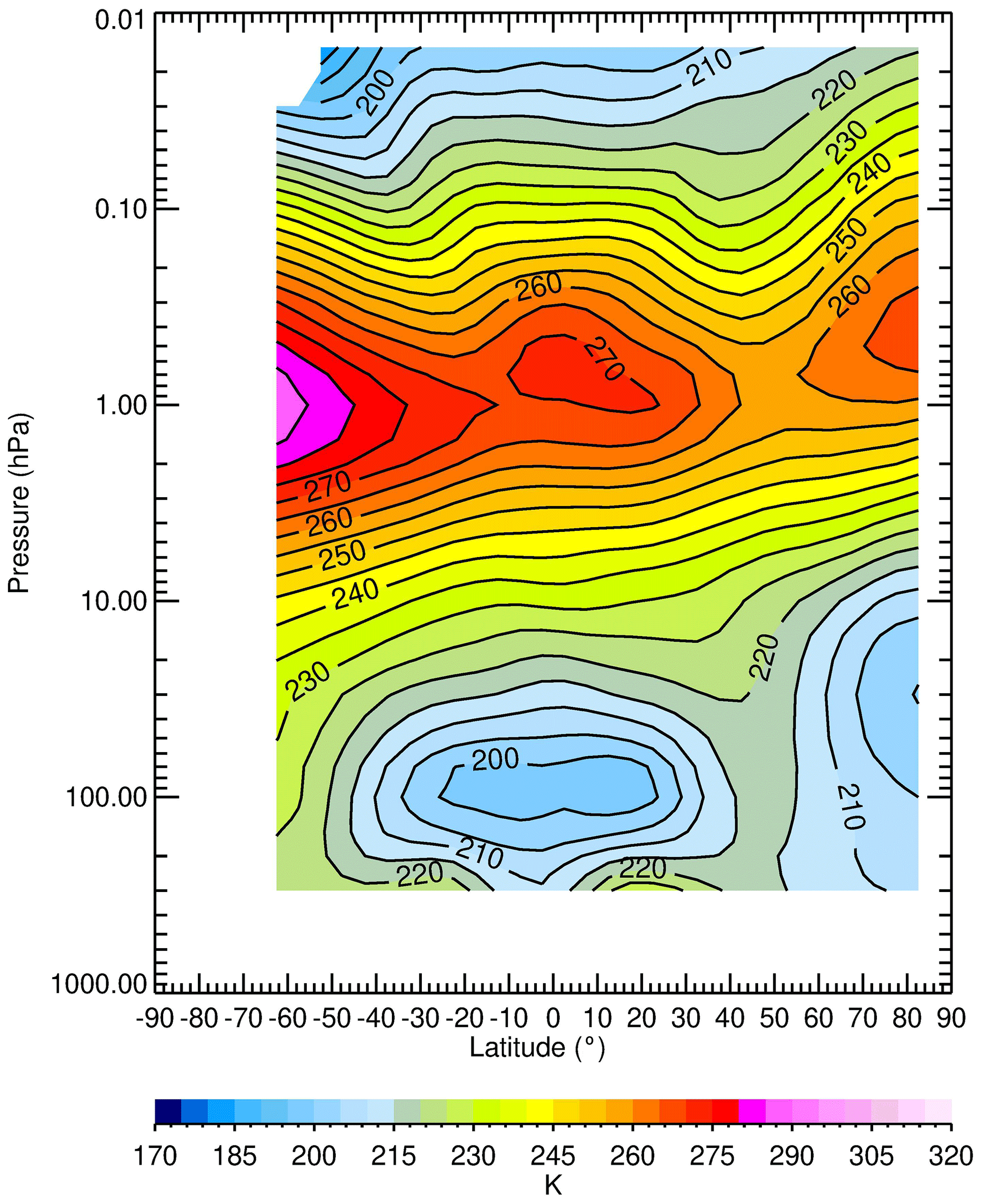
Figure 3 shows the monthly average, zonal (wave) standard deviations (SD) about daily zonal means of the combined-mode (A+D) V6 ozone for January, where the SD values are derived from the zonal-wave amplitudes of V6 Level 3. There are relatively small SD values at low latitudes from 7 to 10 hPa; it is assumed that they are a result of smaller-amplitude Kelvin and Rossby gravity waves. Effects of more vigorous, planetary wave activity are most apparent at high northern latitudes of the stratosphere during winter. Gravity waves also contribute to SD in the uppermost mesosphere (Siskind et al., 2021). Ozone shows little zonal variation in the SH upper stratosphere of Fig. 3, due to constraints on the upward propagation of planetary waves through the summer zonal easterlies (Andrews et al., 1987). SD values near the tropical tropopause are due mostly to residual effects of emissions from thin cirrus and represent spurious ozone variations (see Sect. 6).

Figure 3 Zonal standard deviation about average (A+D) zonal mean ozone for January 1979. CI is 0.075 ppmv.

3 V6 comparisons with rocket-borne chemiluminescent ozone measurements

In this section we consider V6 comparisons with three nighttime, rocket-borne chemiluminescent ozone soundings of Hilsenrath (1980) – one at White Sands, NM, (32.4^∘ N, 253.5^∘ E) on 15 December 1978 and two more at Poker Flat, AK, (65.1^∘ N, 212.5^∘ E) on the successive days of 27 and 28 January 1979. The estimated total rocket ozone error is 14 % (precision plus accuracy), according to Hilsenrath and Kirschner (1980).

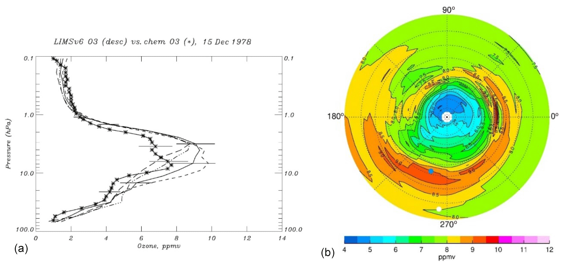
Figure 4 (a) Profiles of V6 ozone (at 06:11 Z) versus rocket chem ozone (* at 05:41 Z) on 15 December. The four V6 profiles have separations of 2.6^∘ latitude, and the solid curve (at 31.8^∘ N) is closest to White Sands (WS, 32.4^∘ N). Horizontal bars are ozone errors. (b) NH V6 ozone at 4.6 hPa; Greenwich (0^∘ E) is on the right, and CI is 0.5 ppmv. Latitude (dotted circles) is every 10^∘. Satellite location is the white dot (6^∘ N, 265^∘ E), and WS is the blue dot.

Ozone comparisons for 15 December are in Fig. 4a; we plot every other V6 profile, and those four profiles have spacings of 2.6^∘ in latitude. The short-dashed V6 profile is at 29.2^∘, and the long-dashed profile is at 37.2^∘. The solid curve is the V6 profile at 31.8^∘ (at 06:11 Z) or closest to the rocket sounding from White Sands (at 05:41 Z). Horizontal bars on the profiles are estimates of ozone error; they overlap between V6 and rocket, except in the upper stratosphere. LIMS ozone is larger than rocket ozone through the upper stratosphere. The corresponding V6 ozone map at 4.6 hPa in Fig. 4b reveals an ozone maximum just south of White Sands (WS – blue dot), along the descending orbital segment of the satellite at 6^∘ N, 265^∘ E (white dot) or viewing in the NNW direction toward White Sands. Note that while zonal variations in the map are from a gridding of the Level 3 coefficients (2^∘ latitude and 5.625^∘ longitude), there is no smoothing of the gridded field in the meridional direction; there is good continuity across latitudes, nonetheless. The rocket profile is a local measurement and has a vertical resolution that ranges from 1.5 km at 60 km to 0.1 km at 20 km; the nearby V6 profiles have a lower vertical resolution of ∼ 3.7 km and are an average over the finite horizontal length (∼ 300 km or ∼ 3^∘ latitude) of the LIMS tangent layer. There is an ozone maximum along the LIMS view path just to the south of White Sands, which may account for the profile differences. We also note that the ozone field of 2 d earlier has the region of sharp gradients positioned over White Sands with ozone at only 8 ppmv. Thus, an ozone field that varies in both space and time can lead to additional uncertainties for comparisons of the localized rocket and limb-viewing satellite profiles in Fig. 4.

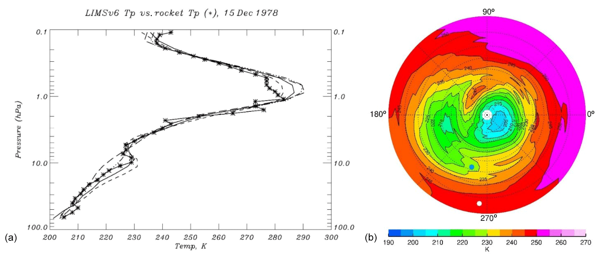
Figure 5 (a) Profiles of V6 temperature compared with datasonde values (*) on 15 December. The four V6 profiles are separated as in Fig. 4, where the short-dashed curve is for 29.2^∘ and the long-dashed curve is for 37.2^∘. (b) NH V6 temperature distribution at 4.6 hPa; CI is 5 K; satellite location is the white dot, and White Sands is the blue dot.

Because V6 ozone is obtained from retrievals of the measured V6 ozone radiance profiles, the LIMS retrieved temperature profile must be representative of the atmospheric state for the forward model of ozone radiance. Figure 5a shows the corresponding temperature comparisons between V6 and a separate rocket datasonde instrument. Agreement between them is very good throughout the upper stratosphere, indicating that the temperature variations are well determined along the LIMS view path for the forward radiance calculations of V6 ozone and that the retrieved V6 ozone should be nearly unaffected by temperature bias error. The map of V6 temperature (Fig. 5b) shows zonal variations on 15 December, although their meridional gradients are relatively weak above White Sands. Conversely, the ozone profiles agree well near 0.68 hPa in Fig. 4, where there are apparent biases between the T(p) profiles. There are significant horizontal gradients near White Sands in the maps of T(p) at 0.68 hPa but not in ozone (not shown). In fact, the V6 ozone field at that level has a nearly constant value, and ozone is less sensitive (by half) to changes in T(p) at 0.68 hPa than at 4.6 hPa (Remsberg et al., 2007). Co-location is more important for the V6 versus rocket comparisons of T(p) than of ozone in the lower mesosphere.

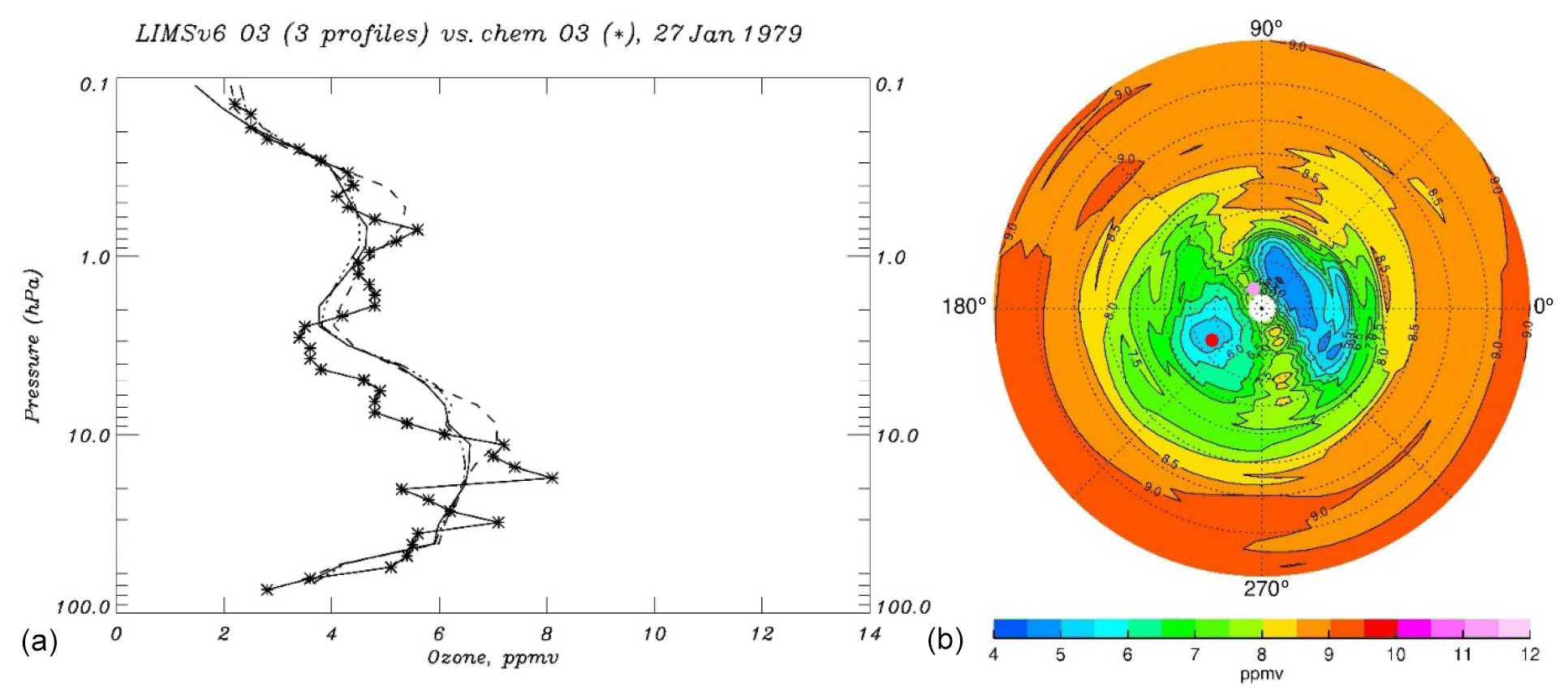
Figure 6 (a) As in Fig. 4 but for 27 January 1979 at Poker Flat, AK (65^∘ N, 212.5^∘ E); (b) NH V6 distribution of ozone at 4.6 hPa, where CI is 0.5 ppmv. Latitudes (dotted circles) are spaced every 10^∘; Poker Flat is red, and satellite position (81^∘ N, 113^∘ E) is pink.

The two comparisons above Poker Flat, AK, occurred at the time of a stratospheric, zonal wave 1 warming event. Leovy et al. (1985) provide a detailed discussion of the advective changes for ozone in the middle stratosphere during January 1979. Figure 6a shows three V6 ozone profiles from along an ascending orbital segment on 27 January. The LIMS instrument was viewing from its satellite location (80.7^∘ N, 113^∘ E) at 22:04 Z, and the rocket ozone launch was 2 h earlier or at 20:05 Z at a solar zenith angle of 84^∘ or near the terminator; there is good agreement of the structure between them, even in the mesosphere. A second rocket launch followed at 08:33 Z of 28 January (Hilsenrath, 1980). Since the separate V6/rocket ozone and T(p) comparisons are similar for the 2 d, Fig. 6 contains results for 27 January only. The rocket sounding recorded two ozone maxima, one near 15 hPa and another at about 0.6 hPa. The ozone maximum at about 15 hPa is primarily due to advection of ozone of higher mixing ratios from lower latitudes just prior to the warming event. The local maximum at 0.6 hPa was unexpected, based on findings from a larger set of rocket ozone soundings. There is a relative minimum for both V6 and rocket ozone through the upper stratosphere, although V6 ozone is larger. The map of V6 ozone at 4.6 hPa in Fig. 6b indicates that the rocket measurement occurs at the center of the minimum, whereas the V6 profiles are averages across it. The ozone profiles in Fig. 6a indicate the relative minimum in a low-ozone pocket (LOP) that extends from about 7 to 2 hPa.

Figure 7 (a) As in Fig. 5 but for 27 January 1979. (b) NH V6 temperature; CI is 5 K. Poker Flat is blue, and satellite position is pink. (c) V6 GPH; CI is 0.375 gpkm (geopotential kilometer).

Figure 7a shows the V6 temperature profile comparisons; T(p) from the datasonde has more vertical structure, as expected from a localized measurement. V6 T(p) values reach a maximum of order 250 K at about 3 to 4 hPa. They agree reasonably with the datasonde values, given that there is significant horizontal structure in the temperature field surrounding Poker Flat. The apparent V6 minus datasonde bias of order 5 K at 3 hPa ought to lead to a V6 minus rocket ozone bias of −40 %, according to error estimates for retrieved V6 ozone. However, Fig. 7b indicates that LIMS was viewing Poker Flat across an area of higher temperatures, such that it is likely that there is a spatial mismatch for V6 and datasonde T(p) values. The much smaller and positive ozone differences in Fig. 6 support that likelihood. There may also be co-location differences between the rocket temperature and ozone soundings in this instance.

Figure 7 also shows a map of NH GPH at 4.6 hPa on 27 January for comparison with the ozone map in Fig. 6. Lowest ozone values are in the polar vortex, where the GPH field is asymmetric about the pole. A second, low value of ozone is associated with the anticyclone over the Alaskan sector. One can determine horizontal winds from gradients of GPH on the 4.6 hPa surface and thereby estimate the transport of ozone to first order. Qualitatively, the direction and strength of the large-scale transport follows from the character of the cyclonic and anticyclonic features on the GPH map. The large-scale cyclonic circulation about the vortex transports air from middle latitudes to across the pole on 27 January. The vortex region has low ozone and is relatively cold, whereas stratospheric temperatures over Alaska show a maximum (the SSW), and the rocket profile above Poker Flat, AK, was near the center of the anticyclone and in the region of relatively low ozone (or LOP).

Ozone is an approximate tracer of transport processes and reveals dramatic changes with altitude associated with this SSW event, even through the winter lower mesosphere. As an example, Fig. S1 (in the Supplement) shows a concurrent cooling at 0.46 hPa above the Alaskan anticyclone on 27 January, where the co-located ozone field exhibits a local maximum. There is also a major temperature increase above the polar stratospheric vortex over northern Europe at 0.46 hPa or where ozone values remain low. In summary, Figs. 4 through 7 and S1 indicate the utility of daily maps from LIMS for analyses of the ozone fields during dynamically disturbed conditions.

4 Variation of a low-ozone pocket (LOP) from LIMS Level 3

The polar vortex on 27 January was located over northern Europe and Asia; it was centered off the pole because of effects of large-scale planetary waves in the development of the SSW (Andrews et al., 1987, chap. 6). In this section, we show sequences of polar plots of both stratospheric GPH and ozone for February 1979. Manney et al. (1995) and Harvey et al. (2004, 2008) provide comprehensive analyses about the occurrence of polar anticyclones and their associated LOPs from studies of GPH and ozone fields from several different satellites. They determined the extent and character of the polar vortex based on meteorological data from the UK Met Office or as obtained from relatively low vertical resolution radiance profiles from operational, nadir temperature sounders. The V6 GPH profiles are derived from and have the same vertical resolution as the T(p) profiles. Manney et al. (1995) showed that water vapor is a useful tracer of the meridional transport of air, and the V6 H₂O fields at 6.8 and 10 hPa indicate that low-latitude air was transported to the region of the LOP in late January. But the V6 H₂O fields are noisy at 4.6 hPa (not shown). Even so, the V6 Level 3 ozone, T(p), and GPH data offer useful details about the occurrence of LOPs in the upper stratosphere.

Figure 8 NH V6 GPH at 4.6 hPa; CI is 0.375 gpkm. Poker Flat is the blue dot. Panels are spaced 1 week apart: (a) 3 February, (b) 10 February, and (c) 17 February.

Harvey et al. (2004) reported that LOPs occur nominally at about the 5 hPa level. Accordingly, the three panels of Fig. 8 show three daily NH maps of V6 GPH from 3 to 17 February at 4.6 hPa; each successive map is spaced 1 week from the previous one. This sequence shows that both the vortex and anticyclone weaken during the 3 weeks following 27 January at this level. The vortex re-centers on the pole by 17 February, and the anticyclone is nearly absent at 4.6 hPa following the two minor warming events. The map sequence of GPH indicates that there were significant changes in the horizontal transport of ozone in late January/early February. The corresponding three panels of ozone in Fig. 9 show the further evolution of ozone, following that of 27 January (in Fig. 6). Even though the anticyclone had weakened during the first week, there was a deepening of the LOP from 27 January to 3 February and a filling of it thereafter.

Figure 9 Maps of ozone at 4.6 hPa (a) on 3 February, (b) on 10 February, and (c) on 17 February. CI is 0.5 ppmv, and the red dot is Poker Flat.

Was there some chemical loss of ozone from 27 January to 3 February in the region of the LOP? Morris et al. (1998) and Nair et al. (1998) conducted model calculations to show how that could happen. Ozone reactions are affected by changes with latitude of solar insolation, temperature, and loss via NO_x. Nair et al. (1998) reported on the effect of a decrease in the production of ozone for the development of LOPs, as air parcels in the middle stratosphere move from low to high latitudes or to higher solar zenith angles in winter. Remsberg et al. (2018) analyzed air parcel trajectories that included chemistry, and they showed that there was some loss of ozone in the middle stratosphere, due to reactions with NO_x. However, Holt et al. (2012) analyzed V6 NO₂ in the winter polar vortex, and they did not find enhanced values at 4.6 hPa due to energetic particle precipitation (EPP) by late January.

Figure 10 (a) Nighttime NO₂ on 27 January at 4.6 hPa; CI is 1.25 ppbv. (b) HNO₃ at 4.6 hPa; CI is 0.375 ppbv. Red dot is Poker Flat.

Figure 10a is a map of the V6 descending orbital (nighttime) NO₂ for 27 January at 4.6 hPa. Based on the corresponding map of GPH in Fig. 7, one can trace the horizontal advection of high NO₂ toward higher latitudes and toward the polar vortex as well as the advection of low NO₂ out of the vortex and about the anticyclone. Figure 10b is a map of HNO₃ at 4.6 hPa, and it shows a weak, relative maximum above the anticyclone.

The formation of the LOP at 5 hPa near Poker Flat region in January is studied with the help of photochemical calculations along a trajectory. A full description of the trajectory and photochemical models is given in Remsberg et al. (2018). For this study, we generated backward trajectory starting at 5 hPa and 212^∘ E and 64^∘ N. The starting time of the back trajectory is 09:00 Z on 28 January 1979. This is close to local time of LIMS descending-mode observation of around 23:00 on 27 January. Figure 11 shows the back trajectory with the day numbers illustrating the progress of the air parcel. Between 22 and 28 January, the air parcel remains confined within a small region at high latitude. Results of a time-dependent photochemical calculation conducted along this trajectory in the forward direction are shown in Fig. 12 as a function of time. The model initialization uses the mixing ratios of O₃, NO₂, and HNO₃ from LIMS descending-mode observations. Figure 12 shows that the parcel was at 3 hPa on 15 January and descended steadily to 5 hPa by late January. The decrease in ozone during the last 8 d is mainly caused by the daytime odd oxygen loss due to the catalytic cycle involving NO_x. Production of odd oxygen is minimized since the air parcel is confined to high latitudes. Large diurnal variations in NO₂ and a small increase in HNO₃ are as expected for this pressure level. The LOP formation is a result of the interplay between transport and photochemistry in the high-latitude upper stratosphere in the winter.

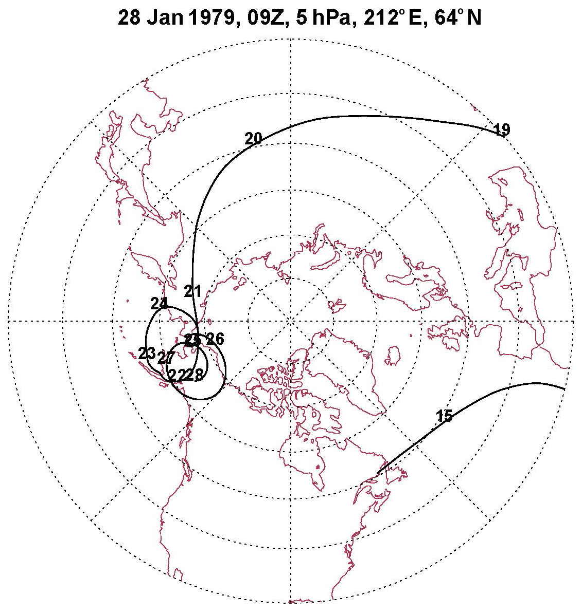
Figure 11 Trajectory of air parcel that ends on 28 January at the location of the LOP. Numbers on the trajectory denote the date, beginning with 15 January, and where the parcel is equatorward of 30^∘ N on 16–18 January.

Figure 12 Air parcel history of the changes in its (a) pressure, (b) ozone, (c) NO₂, and (d) HNO₃.

5 Variations of the tertiary ozone maximum

Smith et al. (2018) describe the changing monthly, zonally averaged character of the wintertime tertiary ozone maximum of the polar upper mesosphere. They point out that the low-latitude edge of the tertiary ozone maximum is where HO_x radicals and the chemical loss of ozone due to reactions with them are reduced. V6 ozone radiance profiles have a low signal-to-noise ratio in the upper mesosphere; the precision estimate is 0.32 ppmv for retrieved ozone profiles. We show a map in Fig. 13 of the combined V6 ozone for 15 December at 0.022 hPa (∼ 72 km), where its distribution in the subpolar region is based on fewer than 13 zonal coefficients because some profiles do not extend to that pressure altitude. The corresponding map of temperature is also in Fig. 13, and one can see that there is significant non-zonal structure in its field at the latitudes where ozone is enhanced. While both V6 ozone and temperature are not highly accurate due to NLTE effects in the upper mesosphere, their maps reveal significant relative spatial structures indicating advective transport and its likely effects on ozone.

Figure 13 NH distributions for 15 December at 0.022 hPa for (a) ozone and for (b) temperature; CIs are 0.5 ppmv and 5 K, respectively. Red dot denotes location of Poker Flat.

Figures S2 and S3 in the Supplement show additional panels at 0.022 hPa of ozone and temperature, respectively, for 13 January, 10 February, and 1 March. Elevated values of ozone occur at higher latitudes on 10 February and 1 March than on 15 December and 13 January, which is consistent with the more northward position of the terminator away from the winter solstice and the consequent effects for the chemical loss of ozone. The temperature fields are also perturbed on 13 January and 10 February, but they are more nearly zonal by 1 March. However, there are meridional gradients of temperature on all 3 d in the region of the tertiary ozone maximum. On 13 January there is also a well-defined mesospheric vortex in GPH (not shown), and the highest values of ozone correlate reasonably with it. The vortex is most disturbed, and tertiary ozone maximum has the largest values on 10 February, perhaps in response to the upward propagation of wave activity following the minor SSW of late January.

Figure 14 shows time series of peak zonal mean ozone at 0.022 hPa and its latitude location for each week from November through mid-March. The separate time series are for peak ozone (bottom two series) and their latitude locations (top two). Dashed red curves represent zonal mean results for combined (A+D) ozone; solid black curves are results for nighttime (D) only. Blue horizontal lines represent the approximate latitude position of the terminator. Peak nighttime ozone values are based on just the zonal mean and the cosine and sine coefficients for waves 1 and 2 because not all profiles reach the 0.022 hPa level. Peak ozone occurs at lower latitudes (∼ 65^∘ N) in December, increasing to ∼ 75^∘ N in early November and early February and to near 80^∘ N by early March. The latitude time series of peak ozone values is reasonably coincident with the changing location of the terminator. Peak combined (A+D) ozone increases slowly from a minimum of 2.2 ppmv in November to 3.6 ppmv in late February and March. Descending (or nighttime only) ozone varies from 3.3 ppmv in November to ∼ 4.5 ppmv in January to a maximum of 6.3 ppmv in mid-February and then declines to 3.5 ppmv by mid-March, although the time series shows rather large variations. Those maximum V6 values are larger than reported by López-Puertas et al. (2018, their Fig. 15), perhaps due to biases from V6 T(p) and/or ozone at 0.022 hPa.

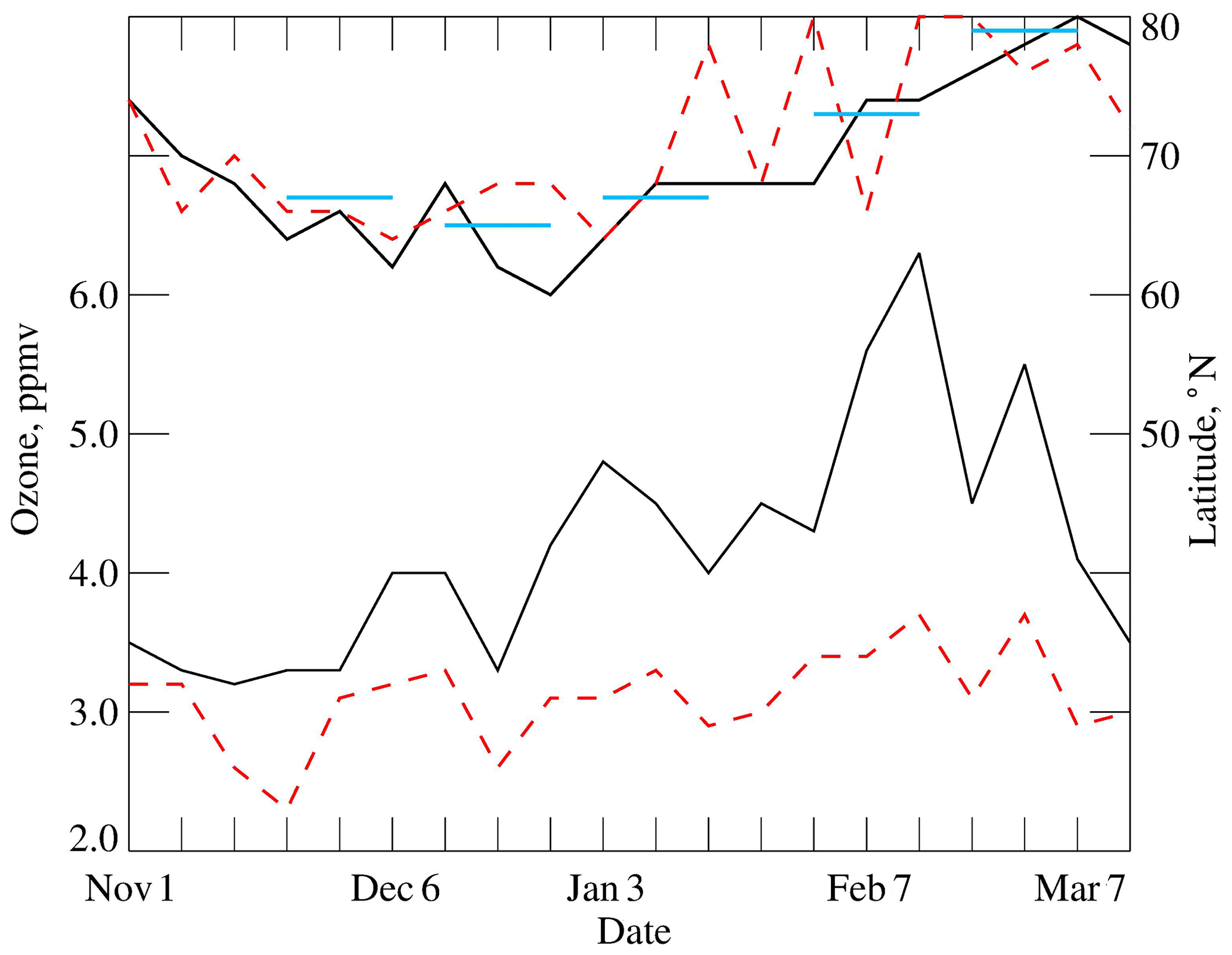
Figure 14 Time series of peak V6 ozone (bottom two curves) and its latitude location (top two curves) at 0.022 hPa. Dashed red curves are for combined ozone, while solid curves are for descending (nighttime) ozone only. Horizontal blue lines indicate the latitude of the terminator.

The increase in V6 ozone during winter in Fig. 14 disagrees with that of Smith et al. (2018), who found decreasing ozone by February. They reported that, in most years, there is a slow descent of relatively dry air into the vortex region in the upper mesosphere during late autumn and early winter and that the reduction in water vapor implies that there are fewer HO_x radicals for the destruction of ozone near the terminator zone, leading to accumulations of ozone. However, there were two minor warmings and associated lower mesospheric cooling events during late January and early February 1979 (Hitchman et al., 1989). The enhanced V6 ozone of February 1979 follows those SSW events, and there are wave-driven disturbances and dissipation of their energy in the upper mesosphere at that time (e.g., Siskind et al., 2005; Smith et al., 2009). One can gain more details about the evolution of the tertiary ozone maximum in the winter of 1978–1979 from the daily maps of V6 ozone, T(p), and GPH (as in Figs. S2 and S3).

6 Other aspects of V6 Level 3 ozone

The combined (A+D) Level 3 coefficients are the basis for a gridding of daily synoptic maps at 12:00 Z of ozone and related parameters. The Level 3 product also contains coefficients from its separate A and D profiles; their zonal mean values correspond to the local time of day of their respective measurements. Remsberg et al. (2007) noted that maps from V6 reveal more details about the variations of ozone. In Fig. S4 of the Supplement we compare a map of V6 ozone at 10 hPa on 27 January with a similar map for V5 of Leovy et al. (1985). The ozone gradients are more pronounced with V6 than with V5 at both the subtropical and vortex edges of the ozone field. The V6 maps make use of all profiles along the orbit, and the SE mapping algorithm was applied to them every 2^∘ of latitude. However, the tighter gradients were also achieved with the V6 algorithm because it has a relaxation time (or memory) that is half that of V5. This means that the V6 maps are more representative of the rapidly changing atmospheric ozone fields on that day. Similar version differences are evident throughout winter, when the so-called “stratospheric surf zone” develops and expands (Leovy et al., 1985).

Significant exchanges of air and ozone occur from the extratropical stratosphere to the troposphere in winter and spring (Gettelman et al., 2011). There are large zonal variations about the daily zonal means of ozone in the Arctic region of the lower stratosphere in Fig. 3. There are similar variations in GPH (and derived winds) and in zonal-wave activity that lead to ozone transport. Zonal variations are resolved in the daily ozone maps down to the 146 hPa level. Notably, Shepherd et al. (2014) integrated the V6 monthly zonal mean ozone above the tropopause and subtracted it from observed total ozone, as part of their assessment of long-term trends of tropospheric ozone from models. Their determination of extratropical tropospheric ozone based on LIMS agrees with that obtained from other ozone datasets.

There is also a relative excess of SD ozone values in Fig. 3 centered at 68 hPa at tropical latitudes, and similar anomalies occur in other LIMS months (not shown). As an example, Fig. 15 shows a map of V6 ozone at 68 hPa (∼ 18 km) on 15 December to give more insight about the source of the tropical variations. Ozone mixing ratio values in Fig. 15 are of order 2 to 3 ppmv at high latitudes, becoming much smaller in the subtropics. However, there is also an unexpected, high value of 2 to 3 ppmv at about 15^∘ N, 150^∘ E. Limb measurements in the ozone channel include radiance effects from cirrus particles that can occur along the tangent view path, although the retrieved ozone mixing ratio profiles were screened of those effects to first order (Remsberg et al., 2007). Even so, we note that ozone is easily affected by any excess radiance because of highly non-linear effects for retrievals of ozone in the lower stratosphere. It is very likely that the anomalous ozone at 68 hPa is a result of residual effects from subvisible cirrus, which is nearly ubiquitous over the western tropical Pacific region (see SPARC, 2006, their Fig. 1.8). While individual V6 ozone profiles may include such spurious features in the tropics, the Level 3 ozone product at 68 hPa is affected mainly when there is an organized convection and outflow of air that persists for several days. The adjacent map of ozone at 46 hPa appears unperturbed in that region (not shown), and tropical ozone at 100 hPa approaches zero. There are much smaller anomalies in maps of nitric acid, as its mixing ratio retrieval is very nearly linear. Anomalies are also not so apparent in maps of V6 H₂O at 68 hPa because the cloud screening algorithm for H₂O accounts for the larger vertical field of view and extent in altitude for measurements in the water vapor channel of LIMS. Thus, one must be mindful that the Level 3 product may indicate excess but spurious ozone at 68 hPa in the tropics.

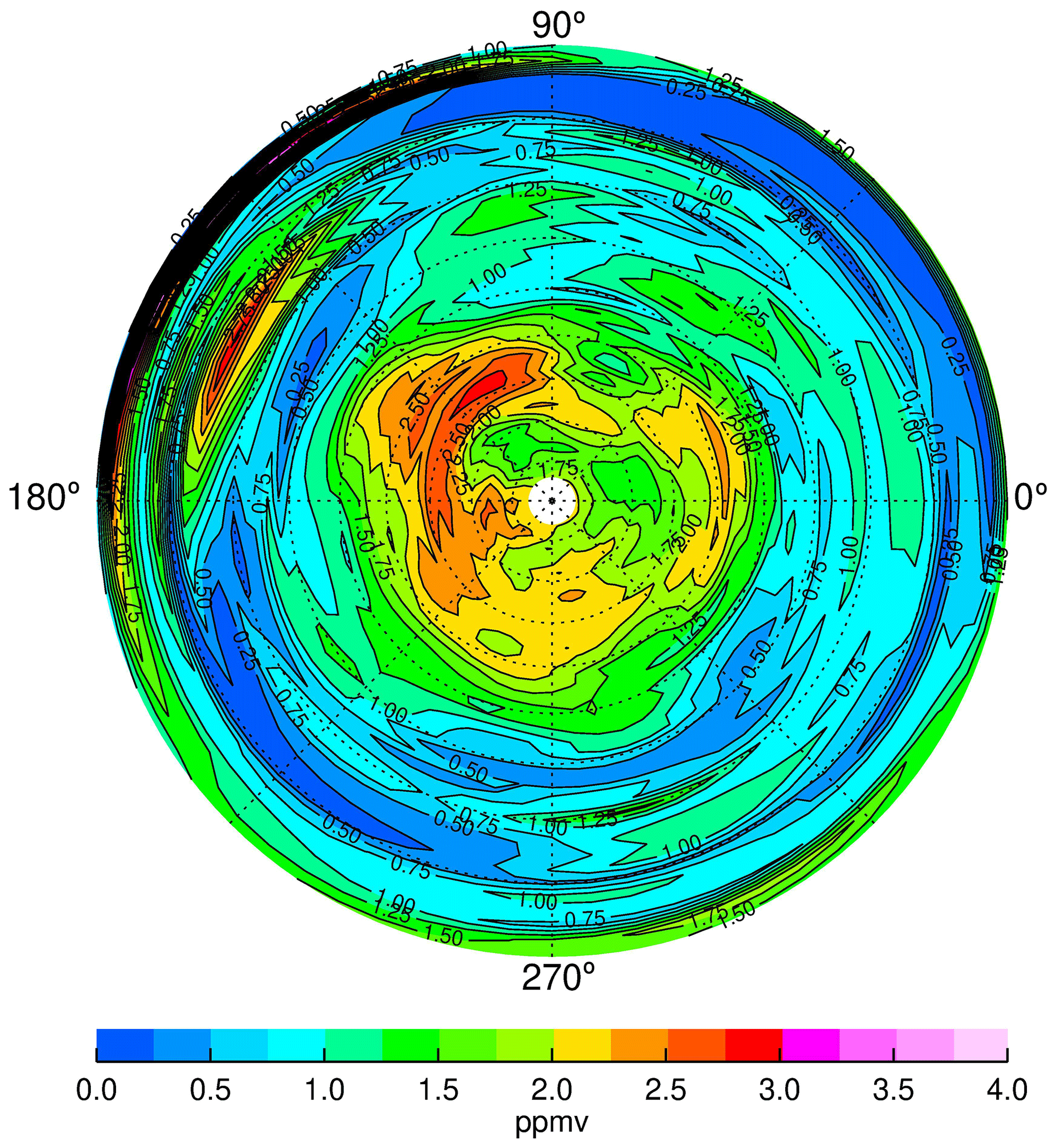
Figure 15 NH V6 combined (A+D) ozone distribution at 68 hPa for 15 December 1978. CI is 0.25 ppmv.

Finally, in our earlier description of descending orbital ozone in Fig. 1, we noted that there are anomalously high values near 45^∘ S in the upper mesosphere. Figure S5 of the Supplement shows distributions of temperature and ozone from descending orbital measurements at 0.032 hPa on 15 January. Zonal-wave activity is very weak in both. The descending orbital views of the tangent layer at 45^∘ S are located in a temperature minimum and just in front of the region of large temperature gradients at 40^∘ S (see also figures in the Supplement of Remsberg et al., 2021). Although we showed in Sect. 3 that taking account of temperature gradients is important for accurate retrievals of ozone, such gradients were not employed for calculations in the mesosphere of tangent layer radiance in the V6 algorithms. If such temperature biases persist through the upper mesosphere, they will also affect the registration of the observed ozone radiance versus pressure at those altitudes. Therefore, we judge that it is very likely that the enhanced ozone mixing ratios near 45^∘ S in Fig. 1 are an artifact because the associated, retrieved tangent path temperatures are not weighted properly, are too cold, and do not account for enough of the observed ozone radiance. Ozone mixing ratio anomalies are not apparent along the ascending orbital segment because their LIMS views are in a near-zonal direction.

7 Conclusions

This report provides guidance to researchers for their use of the LIMS V6 Level 3 product and for their generation of daily gridded distributions of its temperature, ozone, and GPH on pressure surfaces. H₂O, NO₂, and HNO₃ are also available for the stratosphere from the Level 3 product. The V6 dataset represents an early baseline for considering possible changes in the middle atmosphere from 1979 to today and into the future. LIMS made measurements at a time when stratospheric effects from volcanoes were minimal and when catalytic effects of chlorine on ozone were relatively small. Accordingly, Stolarski et al. (2012) found small but significant changes in the distribution of upper stratospheric ozone for recent decades compared with 1978–1979. The LIMS measurements were taken near solar maximum and when atmospheric concentrations of the greenhouse gases (GHG), CO₂, CH₄, and CFCs (chlorofluorocarbons), were smaller than today. Middle atmosphere T(p) distributions were warmer in 1978–1979.

The LIMS measurements in the winter Arctic region occurred when there was a lot of wave activity for the transport and mixing of ozone. As a result, ozone varied dramatically in winter, particularly during times of stratospheric warming events. There was a so-called “Canadian warming” in early December 1978, two minor SSW events in late January and early February, and a final warming in late February 1979. We showed V6 comparisons with temperature and ozone profile data obtained using rocket-borne datasonde and chemiluminescent instruments, and we pointed out how an examination of changes in their nearby fields is valuable for the interpretation and validation of V6 profiles against those correlative measurements. The Level 3 dataset provides daily details on variations of ozone with latitude, longitude, and altitude, along with related variations in temperature, geopotential height, NO₂, and HNO₃. We noted also that there are instances of spurious, excess ozone from the Level 3 coefficients at 68 hPa in the tropics but not in the extratropical stratosphere.

We displayed evidence of a low-ozone pocket (LOP) and its chemical properties at 5 hPa above the Aleutian anticyclone during the minor SSW of late January, and we followed its evolution into mid-February. The V6 nighttime ozone is relatively accurate through the mesosphere in Arctic winter. We provided time series of the wintertime tertiary ozone maximum of the upper mesosphere from V6 data. Its ozone reached maximum values in February, perhaps as a response to enhanced wave activity in the mesosphere following several SSW events. Together with V6 maps of T(p) and GPH, one may explore further the daily evolution of that ozone maximum throughout the NH winter of 1978–1979.