Empirical model of multiple-scattering effect on single-wavelength lidar data of aerosols and clouds

We performed extensive Monte Carlo (MC) simulations of single-wavelength lidar signals from a plane-parallel homogeneous layer of atmospheric particles and developed an empirical model to account for the multiple scattering in the lidar signals. The simulations have taken into consideration four types of lidar configurations (the ground based, the airborne, the CALIOP, and the ATLID) and four types of particles (coarse aerosol, water cloud, jet-stream cirrus, and cirrus). Most of the simulations were performed with a spatial resolution 20 m and particle extinction coefficients ε_p between 0.06 and 1.0 km⁻¹. The resolution was 5 m for high values of ε_p (up to 10.0 km⁻¹). The majority of simulations for ground-based and airborne lidars were performed at two values of the receiver field of view (RFOV): 0.25 and 1.0 mrad. The effect of the width of the RFOV was studied for values up to 50 mrad.

The proposed empirical model is a function that has only three free parameters and approximates the multiple-scattering relative contribution to lidar signals. It is demonstrated that the empirical model has very good quality of MC data fitting for all considered cases.

Special attention was given to the usual operational conditions, i.e. low distances to a layer of partices, small optical depths, and quite narrow receiver fields of view. It is demonstrated that multiple-scattering effects cannot be neglected when the distance to a layer of particles is about 8 km or higher, and the full RFOV is 1.0 mrad. As for the full RFOV of 0.25 mrad, the single-scattering approximation is acceptable; i.e. the multiple-scattering contribution to the lidar signal is lower than 5 % for aerosols (ε_p≲1.0 km⁻¹), water clouds (ε_p≲0.5 km⁻¹), and cirrus clouds (ε_p≤0.1 km⁻¹). When the distance to a layer of particles is 1 km, the single-scattering approximation is acceptable for aerosols and water clouds (ε_p≲1.0 km⁻¹, both RFOV = 0.25 and RFOV = 1 mrad). As for cirrus clouds, the effect of multiple scattering cannot be neglected even at such low distances when ε_p≳0.5 km⁻¹.

1 Introduction

It is well accepted that single-wavelength lidar signals from cloud or aerosol layers are affected by multiple scattering (MS) when the optical thickness is quite high, and/or the distance to a layer is large (see e.g. Winker and Poole, 1995; Bissonnette et al., 1995; and Winker, 2003). A large footprint of the receiver field of view (RFOV) is usually referred to as an intuitive justification of the multiple-scattering importance for signals of spaceborne lidars (see e.g. Winker and Poole, 1995, and Winker, 2003). For example, the Cloud–Aerosol Lidar with Orthogonal Polarization (CALIOP) has a footprint of about 90 m (Winker et al., 2010), which is “roughly two orders of magnitude larger than for ground-based or airborne lidars, due to the large distance from the atmosphere, allowing a much greater fraction of the multiply scattered light to contribute to the return signal” (Winker, 2003). It follows from Monte Carlo simulations of CALIOP signals that multiple scattering is of importance even though photon mean free paths are much larger than the footprint diameter, e.g. cirrus clouds or aerosol layers (see e.g. Winker, 2003).

If the distance to a cloud or an aerosol layer is low, the footprint is rather small. For example, for a typical RFOV of 0.25 mrad and distance to a layer of 8 km, the footprint diameter is 2 m; if the RFOV is 1.0 mrad, the footprint diameter is 8 m. (Note that in this work RFOV refers to the full angle.) If the distance to a layer is 1 km, e.g. an airborne lidar, the footprint diameters become 0.25 and 1 m, respectively. Intuitively, one may expect that the effect of multiple scattering on lidar signals can be neglected with such low footprints and when the extinction coefficient of turbid medium is quite low, for example, 1.0 km⁻¹ or lower. On the other hand, RFOV “can never be infinitely small to satisfy the single-scattering condition” (Bissonnette, 2005). In addition, “the nature of the multiple scattering is fundamentally dependent on the scattering phase function of the atmospheric particles” (Winker, 2003). Thus, the applicability of the single-scattering approximation to lidar signals from layers of large particles, e.g. cirrus clouds, can be suspect.

A number of approximate models, i.e. non-Monte Carlo approaches to simulate lidar signals in multiple-scattering conditions, were developed from the 1970s to 2010s (see e.g. Bissonnette, 2005, and references therein; Eloranta, 1998; Hogan, 2008; and Hogan and Battaglia, 2008). A detailed analysis of those approaches is beyond the scope of this work. We only underscore that they are physically based; that is, some kinds of simplifications and/or approximations are employed, e.g. the time-dependent two-stream approximation (Hogan and Battaglia, 2008). Usually, the approximate models accept varying profiles or multiple layers of cloud and aerosol, and they are very fast as compared to Monte Carlo simulations. Moreover, the corresponding software, e.g. of the models by Eloranta (1998), Hogan (2008), and Hogan and Battaglia (2008), is freely available. At the same time, we believe that the accuracy level and the applicability bounds of the approximate models still need to be rigorously evaluated.

Some works devoted to Monte Carlo (MC) simulations of signals of ground-based lidars were performed from the 1970s to 1990s (see e.g. Plass and Kattawar, 1971; Kunkel and Weinman, 1976; Platt, 1981; Bissonnette et al., 1995; and Ackermann et al., 1999). It was demonstrated that multiple scattering affects lidar signals. At the same time, it should be mentioned that those simulations were performed in conditions that were favourable for multiple scattering: either with a high extinction coefficient (10 km⁻¹ or higher) or with a large RFOV (4 mrad or larger). In the 21st century, the focus of interest of Monte Carlo simulations has mainly shifted to signals from spaceborne lidars.

As for experimental data of ground-based or airborne lidars, it is common practice to assume that multiple scattering is negligible and can be ignored. Usually, that assumption is implicitly implied or mentioned with the relation to the following factors: a narrow RFOV, a small footprint, and a quite low value of the extinction coefficient. The only exception is cirrus clouds observed with a ground-based lidar; that is, the majority of works take into account multiple scattering employing one of the possible multiple-scattering functions (MSFs) (see the discussion in Appendix A) or models (see e.g. Nakoudi et al., 2021, and references therein).

To our knowledge, there exist no works where the applicability of the single-scattering approximation to lidar signals from low distances and low optical depths was thoroughly investigated. Such an investigation is one of the objectives of this work. It was performed using the Monte Carlo technique with special attention to quantitative data.

It follows from our extensive MC simulations that MS relative contribution to lidar signals has the same general behaviour as a function of the in-cloud penetration depth when plotted as a log-linear graph. That property is valid for a wide variety of particle properties, extinction-coefficient values, and lidar configurations (see figures in Sects. 5 and 6 below). Careful analyses of figures published in the literature confirmed that conclusion. The fact that a set of simulated data have the same general behaviour suggests the idea to search for a function which can provide a good fit to the data. Thus, the second objective of this work is to propose and test an empirical model which can be a simple and fast tool to compute multiple-scattering effects on lidar signals.

The organization of this paper is as follows. The methodology and conditions of our Monte Carlo simulations are presented in Sect. 2. Section 3 is devoted to the mathematical background and the analysis of some general features of multiple-scattering impact. Our empirical model of the multiple-scattering effect is discussed in Sect. 4. Section 5 is devoted to results of our MC simulations and fittings with the empirical model for cases of low distances and small optical depths. Section 6 is devoted to cases when the impact of multiple scattering is high, i.e. spaceborne lidars, high values of the extinction coefficient, and wide RFOVs. Some important methodological questions are discussed in Appendices A and B.

2 Methodology and simulation conditions

The principal tool to simulate lidar signals was the McRALI (Monte Carlo Radar Lidar) software developed at the Laboratoire de Météorologie Physique (Alkasem et al., 2017; Szczap et al., 2021). The software employs a forward Monte Carlo (MC) approach along with the locate-estimates method to simulate propagation of radiation (see e.g. Marchuk et al., 2013). McRALI is based on the 3DMCPOL model (Cornet et al., 2010). The polarization state of the radiation is computed using Stokes vectors and scattering matrixes of atmospheric compounds. It takes into account molecular scattering. In this work, the properties of the atmosphere were assigned according to the 1976 standard atmosphere (NOAA, 1976). McRALI is a fully 3D software; that is, values of the extinction coefficients, the single-scattering albedos, and the scattering matrixes are assigned in 3D space. Moreover, the mixture of different types of aerosols and/or clouds is allowed. The position of a lidar can be anywhere within or outside of the atmosphere; that is, spaceborne, airborne, and ground-based measurement conditions can be simulated. A user can assign a lidar beam direction, a RFOV, and a Stokes vector as well as a divergence of the emitted light. It was demonstrated in the work by Alkasem et al. (2017) that McRALI simulations are in good agreement with published results of lidar-signal modelling in multiple-scattering conditions.

Four lidar configurations were taken into consideration in this work. Two configurations were monostatic coaxial zenith-looking lidars, i.e. the ground-based (the altitude is h=0 km) and the airborne (h=7 km), and two values of the RFOV were evaluated for each case, i.e. 0.25 and 1.0 mrad. The emitted light was a linearly polarized delta pulse at a wavelength of λ 0.532 µm. Its divergence was 0.14 mrad. Essentially, we used the characteristics of the lidar system that is in operation at Clermont-Ferrand (Freville et al., 2015). For the sake of brevity, we use the term the “usual operational conditions” (UOCs) when the distance from a lidar to a layer of particles is lower than 15 km, the RFOV ≤ 1 mrad, the emitter field of view (EFOV) ≤ 0.2 mrad, EFOV ≪ RFOV, and the extinction coefficient ε≤1 km⁻¹. All simulations of Sect. 5 were performed for the UOCs.

The other two configurations were spaceborne nadir-looking lidars. We call the “CALIOP configuration” the lidar at an altitude of 705 km having the RFOV 0.13 mrad and the EFOV 0.1 mrad. Only a wavelength of 0.532 µm was considered. We call the “ATLID configuration” (ATmospheric LIDar) the lidar at an altitude of 393 km having the RFOV 0.065 mrad and the EFOV 0.045 mrad (see e.g. Hélière et al., 2012). Only a wavelength of λ=0.355 µm was considered. Note that both configurations should be considered to be proxies for the real lidar systems. The objectives of this work do not require taking into account the pointing off-nadir or the high-spectral-resolution separation of molecular and particulate backscattering (see e.g. Bruneau and Pelon, 2021).

The majority of our MC data were computed so that photons were integrated over a range gate of 20 m; i.e. they correspond to photon counting mode. Such a small value of the range gate was chosen with the aim to study multiple scattering in detail regardless of the fact that it does not correspond to real lidar systems. In other words, the spatial resolution of our data is 20 m. In order to assure good statistical quality of our Monte Carlo modelling, each signal was simulated with 4×10¹⁰ photons emitted by the lidar (with 4×10¹¹ photons for the cirrus clouds having ε=0.06 km⁻¹). Simulations of signals were performed for the orders of scattering n=1 (single scattering); n=2 (double scattering); and multiple scattering with n equal to 20, 40, or 50. (We have verified that the difference between data obtained with n=20 and n=10 was not statistically significant for the majority of the simulation conditions of this work.) In the cases of wide RFOV (Sect. 6.2) and high extinction coefficient (Sect. 6.1.2), 40 and 50 orders of scattering were considered, respectively.

The simulations of this work were performed for four types of particles, namely, a coarse-aerosol layer, a warm cloud, and two types of cirrus clouds. A mixture of particles was not considered. Because Monte Carlo methods are very time-consuming, our study was restricted to the case of the plane-parallel homogeneous layer placed within the altitude h range of 8–11 km. That range was deliberately chosen for all four types of particles despite the fact that it does not correspond to the usual altitudes of coarse aerosols or warm clouds. With such a choice, the phase-function impact on multiple scattering is free of the distance-variation interference. It should be underlined that the results of Sects. 5 and 6 are presented so that they remain unaltered when the lidar pointing angle and/or the layer altitude vary, provided that the distance to the cloud base or border remains unchanged. For example, if a Saharan boundary layer extends from the surface to a range of 3–4.12 km above, and a ground-based lidar is tilted by 68^∘ with respect to the zenith, the curves of Fig. 3a and e can be used to assess MS effects.

The scattering matrixes were computed for the wavelengths 0.355 and 0.532 µm and the values of refractive index corresponding to the published works: (i) ice particles (Warren and Brandt, 2008), (ii) water spheres (IAPWS, 1997), and (iii) coarse-aerosol particles (Dubovik et al., 2002). Knowing that the multiple scattering is fundamentally dependent on the scattering matrix of particles, especially at the small forward and backward angles, and in order to avoid effects due to quantization, all matrixes used in this work were computed with an angular resolution of 0.01^∘ (about 0.175 mrad). In addition, McRALI employs a spline interpolation to compute the cumulative distribution function. That function is used to get a random value of the scattering zenith angle for each scattering event (Cornet et al., 2010). (We have verified that MC simulations were biased when the angular resolution of a scattering matrix was worse than 0.1^∘.)

The single-scattering characteristics of ice particles were computed using the improved geometric optics method (Yang and Liou, 1996); the particles are assumed to be hexagonal ice crystals whose facets have deeply rough surfaces. As a consequence of the surface roughness, the scattering matrix of ice particles has neither halo features (see e.g. Shcherbakov, 2013) nor the delta transmission term (Yang et al., 2013). The size distribution of particles was taken to be the gamma distribution. We have considered two types of cirrus clouds that differ by the value of the effective diameter d_eff. The values d_eff=56.8 µm (the standard deviation 20.1 µm) and d_eff=80.0 µm (the standard deviation 24.5 µm) correspond to the data for jet-stream (JS) cirrus clouds and cirrus clouds (Ci), respectively, of the work by Gayet et al. (2006). The obtained scattering matrixes are in good agreement with the database from Yang et al. (2013). The scattering matrix of the warm cloud was computed according to the Mie theory for water spheres having a gamma size distribution with d_eff=18.0 µm (standard deviation of 5.3 µm). The scattering matrix of the coarse aerosol was simulated according to the work by Dubovik et al. (2006) as the “Mixture 1” of spheroids with the distribution of axis ratios within the range [0.3349, 2.986] (assuming, as the first-order approximation, that shape is independent of size). The size distribution of particles was assumed to be log-normal with a mean radius of 2 µm, standard deviation of 0.6 µm, and d_eff=4.75 µm. That value is in agreement with data of the work by Weinzierl et al. (2009), where it was found that the effective diameter of the Saharan dust showed two main ranges: around 5 and 8 µm. The real and imaginary parts of the refractive index were 1.55 and 0.002, respectively (see e.g. Petzold et al., 2009). To underline the differences in scattering properties, we show, as an example, the normalized phase functions p(θ) for a wavelength of 0.532 µm in Fig. 1 (θ is the scattering angle); their behaviour at forward and backward angles can be seen in the insets.

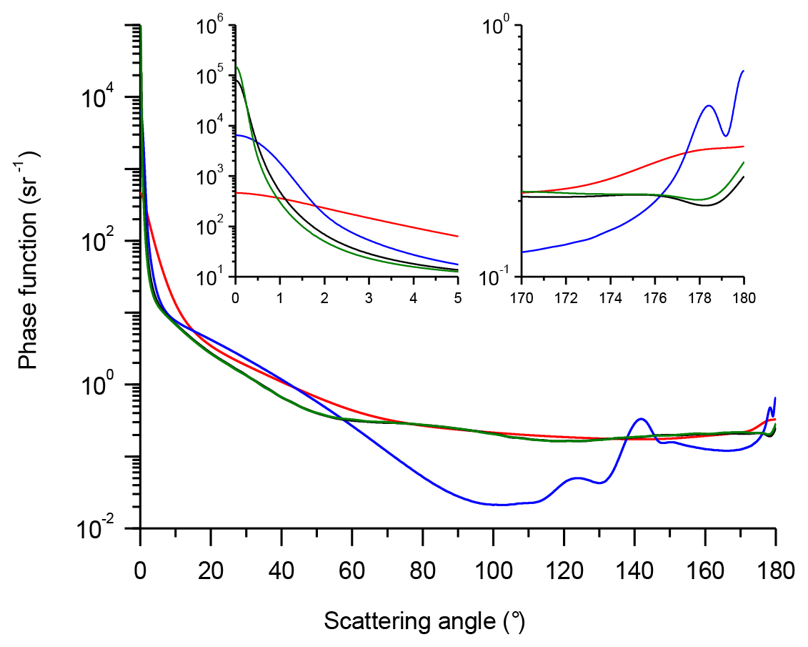
Figure 1 Normalized phase functions: coarse aerosol – red lines, water cloud – blue lines, JS cirrus – black lines, Ci cirrus – green lines.

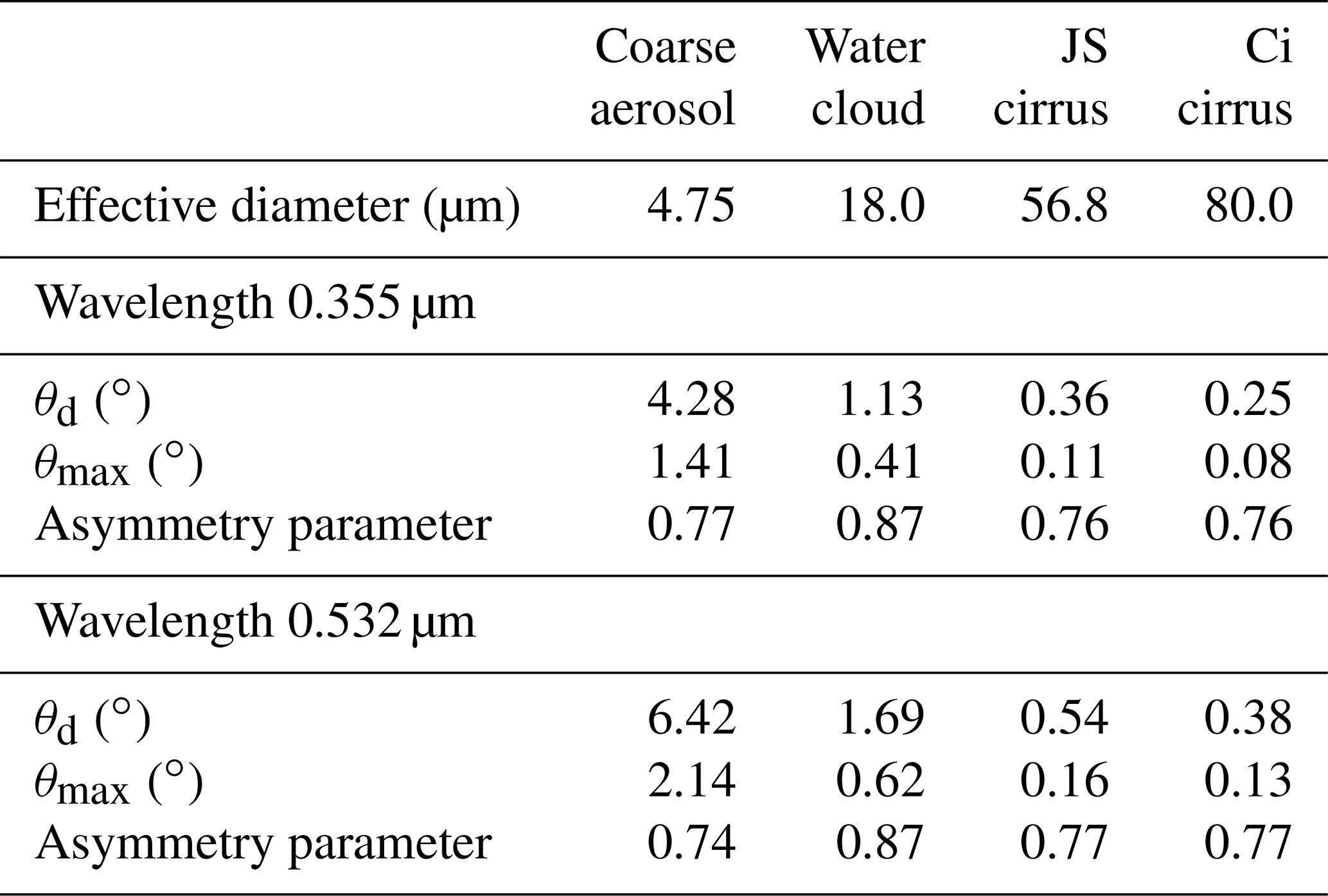
For subsequent discussions, we give in Table 1 parameters that have a significant place in multiple-scattering theory. The effective diameter is usually used to estimate the Fraunhofer diffraction angle ${\mathit{\theta }}_{\mathrm{d}}=\mathit{\lambda }/d_{\mathrm{eff}}$. The asymmetry parameter g, i.e. the first moment of a phase function, is one of the basic parameters of the radiative transfer theory; θ_max is the angle where the function p(θ)⋅sin (θ) takes the maximum. The value of the asymmetry parameter g of the coarse aerosol is quite close to the values observed for ash particles in volcanic degassing plumes (Shcherbakov et al., 2016) and Sahara dust aerosols (Horvath et al., 2018). The values of g for the water cloud and the cirrus cloud are in good agreement with the experimental data of the work by Jourdan et al. (2010).

Table 1 Integral parameters of the phase functions; θ_d is the Fraunhofer diffraction angle, and θ_max is the angle where the function p(θ)⋅sin (θ) takes the maximum.

3 Background and basic properties of multiple-scattering impact

We use the following notations in this work. The function S₁(h) characterizes lidar signals in the single-scattering approximation (corrected for the offset and instrumental factors):

$$\begin{array}{}\text{(1)}& S_{\mathrm{1}}\left(h\right)=\left[{\mathit{\beta }}_{\mathrm{p}}\left(h\right)+{\mathit{\beta }}_{\mathrm{m}}\left(h\right)\right]\cdot T^{\mathrm{2}}\left(h\right),\end{array}$$

where h is the distance from the lidar (the altitude in the case of the ground-based zenith-looking lidar); β_p(h) and β_m(h) represent the backscatter contributions from particles and from the atmospheric molecules; $T^{\mathrm{2}}\left(h\right)=T_{\mathrm{m}}^{\mathrm{2}}\left(h\right)\cdot T_{\mathrm{p}}^{\mathrm{2}}\left(h\right)$ is the two-way transmittance from the lidar to the range h; and $T_{\mathrm{m}}^{\mathrm{2}}\left(h\right)$ and $T_{\mathrm{p}}^{\mathrm{2}}\left(h\right)$ are the molecular and the particulate transmittances, respectively. $T_{\mathrm{p}}^{\mathrm{2}}\left(h\right)=\mathrm{1}$ if h≤h_b, where h_b is the distance to the cloud near end; $T_{\mathrm{p}}^{\mathrm{2}}\left(h\right)=\exp \left[-\mathrm{2}{\mathit{\tau }}_{\mathrm{p}}\left(h_b,h\right)\right]$ when h≥h_b, where ${\mathit{\tau }}_{\mathrm{p}}\left(h_b,h\right)={\int }_{h_b}^h{\mathit{\epsilon }}_{\mathrm{p}}\left(h^{\prime }\right)\mathrm{d}{h}^{\prime }$ is the cloud optical depth, and ε_p(h) is the extinction coefficient of particles.

The term “apparent attenuated backscatter” (see e.g. Chepfer et al., 1999) is employed for lidar signals S_MS(h) computed in multiple-scattering conditions (corrected for the offset and instrumental factors). Without loss of generality, we can assume that

$$\begin{array}{}\text{(2)}& S_{\mathrm{MS}}\left(h\right)=G_{\mathrm{MS}}\left(h\right)\cdot \left[{\mathit{\beta }}_{\mathrm{p}}\left(h\right)+{\mathit{\beta }}_{\mathrm{m}}\left(h\right)\right]\cdot T_{\mathrm{m}}^{\mathrm{2}}\left(h\right)\cdot T_{\mathrm{p}}^{\mathrm{2}}\left(h\right),\end{array}$$

where the multiple-scattering function (MSF) G_MS(h) is the ratio

$$\begin{array}{}\text{(3)}& G_{\mathrm{MS}}\left(h\right)={\displaystyle \frac{S_{\mathrm{MS}}\left(h\right)}{S_{\mathrm{1}}\left(h\right)}}.\end{array}$$

It is employed as a factor that corrects the lidar signal of the single-scattering approximation. Such an approach was used in the automated algorithm of the Atmospheric Radiation Measurement programme's Raman lidar (Thorsen and Fu, 2015). As a matter of fact, Eq. (2) is no more than a mathematical expression that provides an easy way to assign the relationship between S_MS(h) and S₁(h).

A specific model of multiple scattering appears only when G_MS(h) is given in an explicit form. The specific model that is widely used by the lidar community is based on the works by Platt (1973, 1979). It was proposed to account for “secondary scattering or higher order processes” using the factor (in our notations η_MS(h)) that “multiplies the optical depth, has a value less than unity and it may vary with altitude” (Platt, 1979). In that case, lidar signals that have been corrected for the offset and instrumental factors can be written as (Winker, 2003)

$$\begin{array}{}\text{(4)}& \begin{array}{rl}{S}_{\mathrm{MS}}\left(h\right)& =\left[{\mathit{\beta }}_{\mathrm{p}}\left(h\right)+{\mathit{\beta }}_{\mathrm{m}}\left(h\right)\right]\cdot T_{\mathrm{m}}^{\mathrm{2}}\left(h\right)\\ & \cdot \exp ⌈-\mathrm{2}{\mathit{\eta }}_{\mathrm{MS}}\left(h\right){\mathit{\tau }}_{\mathrm{p}}\left(h_b,h\right)⌉.\end{array}\end{array}$$

It is a straightforward matter to transform Eq. (4) to the form

$$\begin{array}{}\text{(5)}& \begin{array}{rl}{S}_{\mathrm{MS}}\left(h\right)& =\left[{\mathit{\beta }}_{\mathrm{p}}\left(h\right)+{\mathit{\beta }}_{\mathrm{m}}\left(h\right)\right]\cdot T_{\mathrm{m}}^{\mathrm{2}}\left(h\right)\cdot T_{\mathrm{p}}^{\mathrm{2}}\left(h\right)\\ & \cdot \exp \left\{\mathrm{2}\left[\mathrm{1}-{\mathit{\eta }}_{\mathrm{MS}}\left(h\right)\right]{\mathit{\tau }}_{\mathrm{p}}\left(h_b,h\right)\right\}\end{array}\end{array}$$

and obtain the relationship

$$\begin{array}{}\text{(6)}& G_{\mathrm{MS}}\left(h\right)=\exp \left\{\mathrm{2}\left[\mathrm{1}-{\mathit{\eta }}_{\mathrm{MS}}\left(h\right)\right]{\mathit{\tau }}_{\mathrm{p}}\left(h_b,h\right)\right\}.\end{array}$$

Equations (3) and (6) lead directly to the well-known formula for the multiple-scattering function (MSF) (Winker, 2003)

$$\begin{array}{}\text{(7)}& {\mathit{\eta }}_{\mathrm{MS}}\left(h\right)=\mathrm{1}-{\displaystyle \frac{\mathrm{1}}{\mathrm{2}\cdot {\mathit{\tau }}_{\mathrm{p}}\left(h_b,h\right)}}\cdot \ln \left[{\displaystyle \frac{S_{\mathrm{MS}}\left(h\right)}{S_{\mathrm{1}}\left(h\right)}}\right],\end{array}$$

which can be rewritten as

$$\begin{array}{}\text{(8)}& {\mathit{\eta }}_{\mathrm{MS}}\left(h\right)=\mathrm{1}-{\displaystyle \frac{\mathrm{1}}{\mathrm{2}\cdot {\mathit{\tau }}_{\mathrm{p}}\left(h_b,h\right)}}\cdot \ln \left[G_{\mathrm{MS}}\left(h\right)\right].\end{array}$$

The relationships between G_MS(h) and two types of MSFs can be found in Appendix A.

The interpretation of MSF η_MS(h) plots should be done with appropriate caution because of the logarithm on the right-hand side of Eqs. (7)–(8). If it is assumed that η_MS(h)=const, and the impact G_MS(h) of multiple scattering has an exponential growth rate as a function of the in-cloud optical depth τ_p(h_b,h) (see Eqs. 3 and 6). If G_MS(h) increases, but with a rate lower than exponential, η_MS(h) increases. That feature is of importance for a complete understanding of the MSF η_MS(h) behaviour at the near end of a layer of particles. If G_MS(h) has a faster-than-exponential growth rate, the MSF η_MS(h) decreases.

Our Monte Carlo simulations provide the range-dependent lidar signals in the single-, the double-, and the multiple-scattering conditions, that is, S₁(h), S₂(h), and S_MS(h) with a spatial resolution of 20 m. The ratio, that is, the relative contribution of multiple scattering

$$\begin{array}{}\text{(9)}& R_{\mathrm{MSto}\mathrm{1}}\left(h\right)=\left[S_{\mathrm{MS}}\left(h\right)-S_{\mathrm{1}}\left(h\right)\right]/S_{\mathrm{1}}\left(h\right)=G_{\mathrm{MS}}\left(h\right)-\mathrm{1},\end{array}$$

can be computed directly from the MC data; R_MSto1(h)=0 if h≤h_b. We recall that R_MSto1(h) is largely used in the literature to address effects of multiple scattering on lidar signals when direct problems are dealt with.

It is instructive to see the double-scattering impact, especially when the multiple-scattering effect is not high. Thus, we use the notations G₂(h), η₂(h), and R_2to1(h) that are computed according Eqs. (3), (7), and (9), respectively, with the difference that S_MS(h) is replaced by S₂(h). MC simulations never provide continuous functions. Quantization of lidar data, in our case, means the integration over a distance interval; that is, a range gate is always required. It is of importance that the MSFs η₂(h_i) and η_MS(h_i) are computed with h_i assigned to the middle of the range gate when Eq. (7) is used (see details in Appendix B).

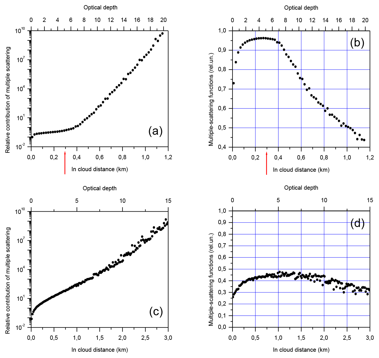
Figure 2 Multiple-scattering contributions R_MSto1 to lidar signals (a, c) and multiple-scattering functions η_MS(d) (b, d). MUSCLE case (a, b), CALIOP case (c, d). The red arrow indicates the far end of the MUSCLE comparison (Bissonnette et al., 1995).

Some important features of the multiple-scattering effect can be revealed when lidar signals are simulated within a quite large range of the optical depth in spite of limitations imposed by technical characteristics of receivers. Figure 2 shows results of two cases that are quite distinguished in terms of the configuration and particle properties. Both simulations were performed with a spatial resolution of 20 m and a total number of photons of 4×10¹⁰; 50 orders of scattering were taken into account.

We used for the first case (Fig. 2a and b) the configuration of the MUSCLE (MUltiple Scattering in Lidar Experiments) community (Bissonnette et al., 1995; Winker and Poole, 1995). The distance to the water cloud C1 is low (h_b=1 km); the lidar transmitter has a wavelength of 1.064 µm and a divergence of 0.1 mrad (full angle); the full RFOV is 1.0 mrad; and the particle extinction coefficient is large (17.25 km⁻¹), which is favourable for multiple scattering. In the work by Bissonnette et al. (1995) the results are shown for penetration depths up to 300 m (${\mathit{\tau }}_{\mathrm{p}}\left(h_b,h\right)=\mathrm{5.175}$). Within that range, the McRALI simulations are in total agreement with the MUSCLE data (see details in Alkasem et al., 2017). In this work, we show our MC data for penetration depths up to 1.15 km (${\mathit{\tau }}_{\mathrm{p}}\left(h_b,h\right)=\mathrm{19.8}$).

The second case (Fig. 2c and d) deals with the configuration of the Cloud–Aerosol Lidar with Orthogonal Polarization (CALIOP) (Winker et al., 2010). The nadir-looking lidar is at an altitude of 705 km; the transmitter has a wavelength of 0.532 µm and a divergence of 0.11 mrad (full angle); the full RFOV is 0.13 mrad. A cirrus cloud (Ci) has an extinction coefficient 5.0 km⁻¹.

To evidence the multiple-scattering effect, two functions are mostly used in the literature, namely, the relative contribution of multiple scattering R_MSto1(h) and the MSF η_MS(h). Both functions are shown in Fig. 2; the red arrow indicates the far end of the MUSCLE comparison (Bissonnette et al., 1995). The literature and our wealth of experience in lidar-signal MC simulations suggest that the function R_MSto1(h) possesses at the near end of a cloud the features which are common for most if not all configurations and particle properties. In the beginning, R_MSto1(h) is linearly proportional to the in-cloud distance (see Fig. 2a and c and the sections below). Then, the curve bends to the right at the in-cloud distance d₁ (d₁≈0.03 km in Fig. 2a and d₁≈0.07 km in Fig. 2c). It continues to increase at the same rate within a quite large range. The curve bends upward at the in-cloud distance d₂ (d₂≈0.52 km in Fig. 2a and d₂≈1.35 km in Fig. 2c), i.e. at an optical depth somewhere between 6.0 and 7.0. The differences in lidar configurations and/or particle properties result in the width of the intervals [0,d₁] and [d₁,d₂] as well as in the increasing rate of R_MSto1(h) within these intervals. We hypothesize that the multiple-scattering effect within the range [0,d₂] is mostly due to the photons that remain within or close to the RFOV; in contrast, the photons that walk a lot outside the RFOV become dominant when d>d₂. (We recall that ${\mathit{\tau }}_{\mathrm{p}}\left(h_b,h\right)\approx \mathrm{7.0}$ is at the bound of technical capacities of contemporary lidars.)

The functions R_MSto1(h) and η_MS(h) have a direct relationship (see Eqs. 8–9). At the same time, the MSF η_MS(h) (Fig. 2b and d) can provide a somewhat more keen insight into effects of multiple scattering. For example, a pronounced change in the η_MS(h) behaviour at an optical depth of ${\mathit{\tau }}_{\mathrm{p}}\left(h_b,h\right)\approx \mathrm{7.0}$ is seen in Fig. 2b, which implies that some other physical events become dominant. In Fig. 2d that property can be observed even though it is less pronounced. All that leads to the conclusion that our empirical model (see below) is limited to the cases when the optical depth ${\mathit{\tau }}_{\mathrm{p}}\left(h_b,h\right)<\mathrm{7.0}$.

4 Empirical model

It follows from our Monte Carlo simulations for different configurations and/or particle properties that the computed functions G_MS(h) show a similar behaviour within the range [0,d] of the in-cloud distance d when plotted as a log-linear graph. (Typical examples can be seen in Figs. 3, 5, and 8.) That similarity led us to the following empirical model:

$$\begin{array}{}\text{(10)}& G_{\mathrm{MS}}\left(d\right)=\exp \left[V(d,\mathbf{a})\right],\end{array}$$

where the function V(d,a)​​​​​​​ has only three free parameters ($\mathbf{a}=\left\{a_{\mathrm{1}},a_{\mathrm{2}},a_{\mathrm{3}}\right\}$), and the domain of definition d≥0

$$\begin{array}{}\text{(11)}& V(d,\mathbf{a})=a_{\mathrm{1}}\cdot \arctan \left(a_{\mathrm{2}}\cdot d\right)+a_{\mathrm{3}}\cdot d.\end{array}$$

If values of V(d,a) are quite small (i.e. the impact of multiple scattering is quite low), we can write using the first two terms of the expansion in powers of V(d,a) of the exponential function

$$\begin{array}{}\text{(12)}& G_{\mathrm{MS}}\left(d\right)=\exp \left[V(d,\mathbf{a})\right]\approx \mathrm{1}+V\left(d,\mathbf{a}\right).\end{array}$$

Equations (9) and (12) lead to the relationship $R_{\mathrm{MSto}\mathrm{1}}\left(d\right)\approx V(d,\mathbf{a})$. Thus, the simplified version of the empirical model can be used to fit simulation data R_MSto1(d) with the function V(d,a). Some properties of V(d,a) can be easily deduced:

$$\begin{array}{}\text{(13)}& V\left(d,\mathbf{a}\right)\approx \left(a_{\mathrm{1}}\cdot a_{\mathrm{2}}+a_{\mathrm{3}}\right)\cdot d=b\cdot d\end{array}$$

at small values of d, i.e. at the cloud near end h_b. In other words, V(d,a) is linearly proportional to the in-cloud distance with the coefficient $b=\left(a_{\mathrm{1}}\cdot a_{\mathrm{2}}+a_{\mathrm{3}}\right)$ and $V(\mathrm{0},\mathbf{a})=\mathrm{0}$.

At large values of d,

$$\begin{array}{}\text{(14)}& V\left(d,\mathbf{a}\right)\approx a_{\mathrm{1}}\cdot {\displaystyle \frac{\mathit{\pi }}{\mathrm{2}}}+a_{\mathrm{3}}\cdot d;\end{array}$$

that is, it is again linearly proportional to the in-cloud distance but with the coefficient a₃.

The function exp [V(d,a)] has the following properties.

$$\begin{array}{}\text{(15)}& \exp \left[V(d,\mathbf{a})\right]\approx \mathrm{1}+\left(a_{\mathrm{1}}\cdot a_{\mathrm{2}}+a_{\mathrm{3}}\right)\cdot d\end{array}$$

at small values of d. At large values of d,

$$\begin{array}{}\text{(16)}& \begin{array}{rl}\exp \left[V(d,\mathbf{a})\right]& \approx \exp \left[a_{\mathrm{1}}\cdot {\displaystyle \frac{\mathit{\pi }}{\mathrm{2}}}+a_{\mathrm{3}}\cdot d\right]\\ & =\exp \left[a_{\mathrm{1}}\cdot {\displaystyle \frac{\mathit{\pi }}{\mathrm{2}}}\right]\cdot \exp \left[a_{\mathrm{3}}\cdot d\right];\end{array}\end{array}$$

that is, it increases exponentially with the in-cloud distance.

It is worthwhile to see how the MSF η_MS(d) is expressed in terms of the empirical model. Equations (8), (10), and (11) lead to the following relationship when ε_p=const:

$$\begin{array}{}\text{(17)}& {\mathit{\eta }}_{\mathrm{MS}}\left(d\right)=\mathrm{1}-{\displaystyle \frac{a_{\mathrm{3}}}{\mathrm{2}\cdot {\mathit{\epsilon }}_{\mathrm{p}}}}-{\displaystyle \frac{a_{\mathrm{1}}}{\mathrm{2}\cdot {\mathit{\epsilon }}_{\mathrm{p}}\cdot d}}\cdot \arctan \left(a_{\mathrm{2}}\cdot d\right).\end{array}$$

Using properties of the arctangent, we can write

$$\begin{array}{}\text{(18)}& {\mathit{\eta }}_{\mathrm{MS}}\left(d\right)\approx \mathrm{1}-{\displaystyle \frac{\mathrm{1}}{\mathrm{2}\cdot {\mathit{\epsilon }}_{\mathrm{p}}}}\cdot \left(a_{\mathrm{1}}\cdot a_{\mathrm{2}}+a_{\mathrm{3}}\right)+{\displaystyle \frac{a_{\mathrm{1}}\cdot a_{\mathrm{2}}^{\mathrm{3}}}{\mathrm{6}\cdot {\mathit{\epsilon }}_{\mathrm{p}}}}\cdot d^{\mathrm{2}}\end{array}$$

at small values of the in-cloud distance d and

$$\begin{array}{}\text{(19)}& {\mathit{\eta }}_{\mathrm{MS}}\left(d\right)\approx \mathrm{1}-{\displaystyle \frac{a_{\mathrm{3}}}{\mathrm{2}\cdot {\mathit{\epsilon }}_{\mathrm{p}}}}-{\displaystyle \frac{\mathit{\pi }\cdot a_{\mathrm{1}}}{\mathrm{4}\cdot {\mathit{\epsilon }}_{\mathrm{p}}}}\cdot {\displaystyle \frac{\mathrm{1}}{d}}\end{array}$$

at large values of d within some range of d<d₂ (see Sect. 3).

Another function exists, which is somewhat similar to arctan (x), namely, the hyperbolic tangent tanh (x). The hyperbolic tangent is frequently used in the radiative transfer theory. Thus, we assayed another empirical model where arctan (x) was replaced by tanh (x). Our tests (not shown here) revealed that the model Eq. (10) always provides fitting errors lower or much lower than the model with the hyperbolic tangent.

The sensitivity of the parameterization to the adjusted parameters $\mathbf{a}=\left\{a_{\mathrm{1}},a_{\mathrm{2}},a_{\mathrm{3}}\right\}$ can be evaluated using the error-propagation formula (see chap. 5 in JCGM, 2008) and Eqs. (10)–(11). The relative error $\mathrm{\Delta }{G}_{\mathrm{MS}}\left(d\right)/G_{\mathrm{MS}}\left(d\right)$ is expressed as

$$\begin{array}{}\text{(20)}& \begin{array}{rl}\mathit{\delta }{G}_{\mathrm{MS}}\left(d\right)& =\mathit{\{}{\arctan }^{\mathrm{2}}\left(a_{\mathrm{2}}\cdot d\right)\cdot {\left(\mathrm{\Delta }{a}_{\mathrm{1}}\right)}^{\mathrm{2}}\\ & +{\displaystyle \frac{a_{\mathrm{1}}\cdot d}{\mathrm{1}+a_{\mathrm{2}}^{\mathrm{2}}\cdot d^{\mathrm{2}}}}\cdot {\left(\mathrm{\Delta }{a}_{\mathrm{2}}\right)}^{\mathrm{2}}+d^{\mathrm{2}}\cdot {\left(\mathrm{\Delta }{a}_{\mathrm{3}}\right)}^{\mathrm{2}}{\mathit{\}}}^{\frac{\mathrm{1}}{\mathrm{2}}},\end{array}\end{array}$$

where Δa_i is the standard uncertainty in a_i. It is seen that δG_MS(d) is continuous in the interval d≥0, increasing with the in-cloud distance d, and $\mathit{\delta }{G}_{\mathrm{MS}}\left(d\right)\approx d\cdot \left|\mathrm{\Delta }{a}_{\mathrm{3}}\right|$ at large values of d.

In this work, all values of the fitting parameters $\mathbf{a}=\left\{a_{\mathrm{1}},a_{\mathrm{2}},a_{\mathrm{3}}\right\}$ are given in the tables in the Supplement to avoid overloading the text.

5 Low distances and small optical depths

For the sake of brevity, we use the term “usual operational conditions” (UOCs) when the distance from a lidar to a layer of particles is lower than 15 km, the RFOV ≤ 1 mrad, the emitter field of view (EFOV) ≤ 0.2 mrad, EFOV ≪ RFOV, and the extinction coefficient ε≤1 km⁻¹. All simulations in this section were performed for the UOCs and at a wavelength of 0.532 µm.

5.1 Ground-based lidar

Figures 3 and 4 show the results of our MC simulations reported in terms of the ratios R_MSto1 and MSF η_MS(d), respectively. The ground-based lidar is at an altitude of h=0 km; the layer is within the altitude h range of 8–11 km. The distance to the layer base is 8 km. The number of photons emitted by the lidar was 4×10¹⁰. We use the same type of notation in both figures. The left-hand column corresponds to the full RFOV of the lidar 1.0 mrad; the right-hand column corresponds to the full RFOV of 0.25 mrad. Blue, red, green, and purple points show the MC simulation results obtained with the extinction coefficient 1.0, 0.5, 0.2, and 0.06 km⁻¹, respectively. The black curves in Fig. 3 represent the fitting results; each curve corresponds to its own set of points R_MSto1(d). The MC data were fitted by the V(d,a) function; that is, we computed the values of the free parameters $\mathbf{a}=\left\{a_{\mathrm{1}},a_{\mathrm{2}},a_{\mathrm{3}}\right\}$ using the ordinary least squares approach.

Figure 3 Multiple-scattering contributions R_MSto1 to lidar signals. Points – MC simulations, black lines – fitting with the empirical model. The full RFOV is 1.0 mrad (a–d) and 0.25 mrad (e–h). Coarse aerosol (a, e), water cloud (b, f), JS cirrus (c, g), Ci cirrus (d, h). The extinction coefficient is 1.0 km⁻¹ (blue points), 0.5 km⁻¹ (red points), 0.2 km⁻¹ (green points), and 0.06 km⁻¹ (purple points). The distance to the cloud base is 8 km.

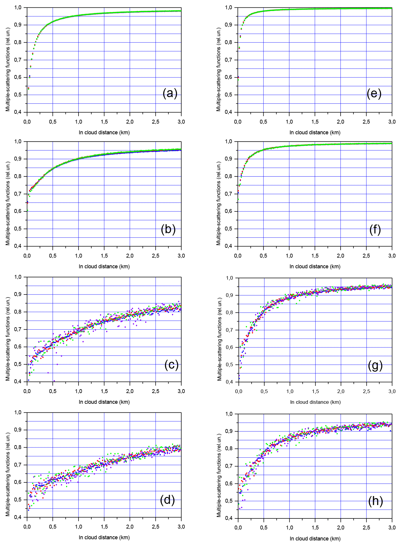
Figure 4 MC simulations of multiple-scattering functions η_MS(d). The full RFOV is 1.0 mrad (a–d) and 0.25 mrad (e–h). Coarse aerosol (a, e), water cloud (b, f), JS cirrus (c, g), Ci cirrus (d, h). The extinction coefficient is 1.0 km⁻¹ (blue points), 0.5 km⁻¹ (red points), 0.2 km⁻¹ (green points), and 0.06 km⁻¹ (purple points). The distance to the cloud base is 8 km.

The cases of the low-value ε_p(h)=0.06 km⁻¹ have the following peculiarities. The double scattering dominates to the extent that higher scattering orders can be neglected. The effect of multiple scattering is very low for the coarse aerosol and the water cloud (therefore, the corresponding data are not shown in this work). As for JS cirrus and Ci cirrus, the corresponding MC simulations were performed with the number of photons emitted by the lidar 10 times higher, i.e. 4×10¹¹, in order to decrease random noise. The difference in the spread of points between the layer types is clearly seen in Figs. 3–8. It is in agreement with the general property of MC simulations of radiative transfer (see e.g. Buras and Mayer, 2011). The stronger the forward peak of the scattering phase function, the slower the convergence of MC simulations is. In other words, the lower value of θ_max, the higher the spread of points is (all other parameters being the same).

It is seen in Fig. 3 that the function V(d,a) fits well with the MC data, which vary widely in terms of values and curve shape. (The corresponding values of the parameters $\mathbf{a}=\left\{a_{\mathrm{1}},a_{\mathrm{2}},a_{\mathrm{3}}\right\}$ are given in Tables S1 and S2 of the Supplement.)

Despite large shape variation in the ratios R_MSto1 in Fig. 3, all curve shapes are in total agreement with the literature. For example, the curves corresponding to the water and cirrus clouds look like curves in the following works (Fig. 5 in Kunkel and Weinman, 1976; Fig. 3 in Wandinger, 1998; Fig. 6 in Eloranta, 1998). As for the ratios R_MSto1(d) corresponding to the coarse aerosol, they are linearly proportional to the penetration depth d starting from about d=250 m. That feature is in agreement with Fig. 2 of the work by Ackermann et al. (1999).

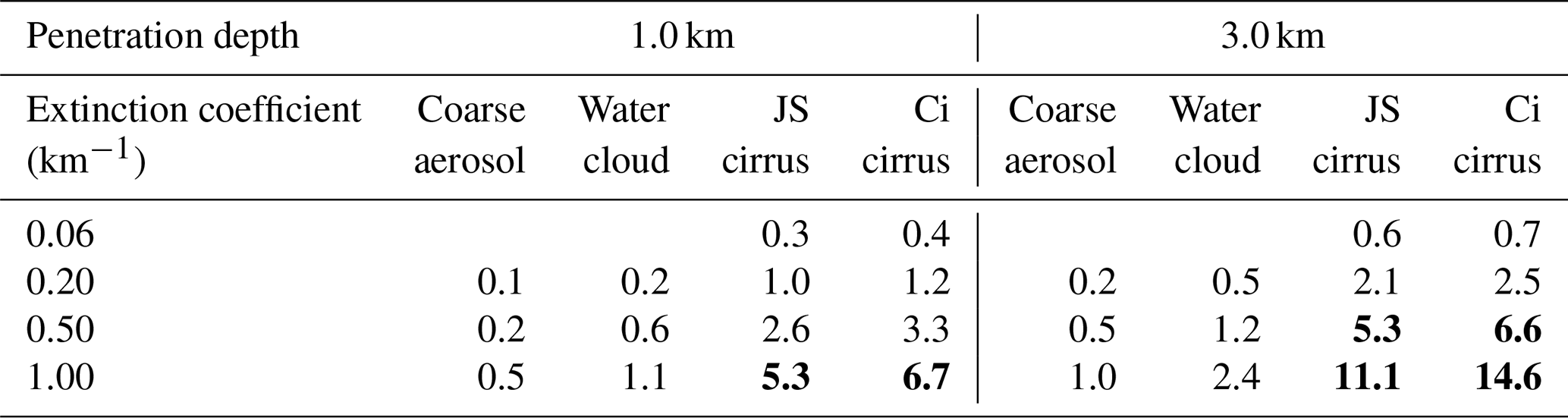
Table 2 Multiple-scattering contribution to lidar signals in per cent (%) of the single scattering. The distance to the cloud base is 8 km; the lidar RFOV is 1.0 mrad. Values exceeding 5 % threshold are in bold font.

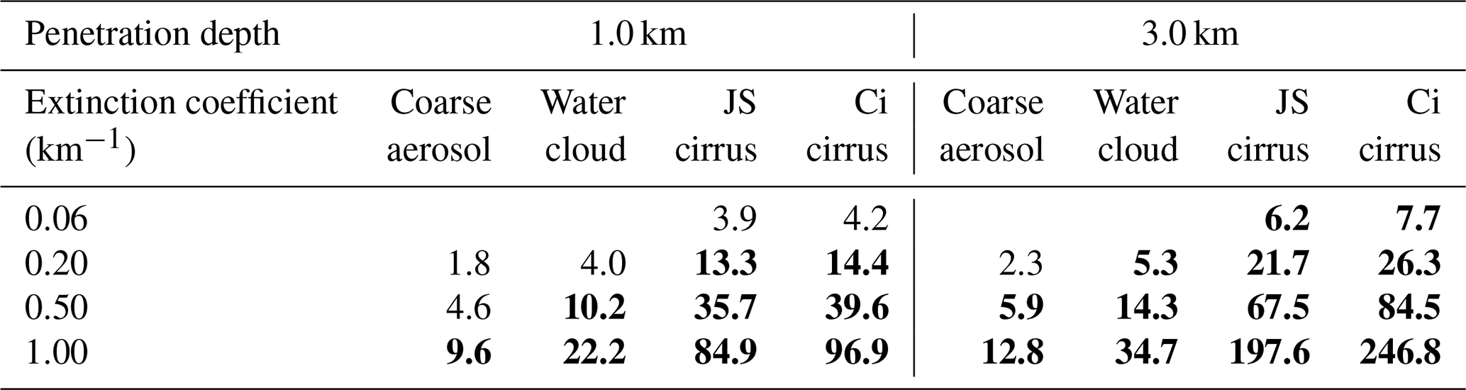
Table 3 Multiple-scattering contribution to lidar signals in per cent (%) of the single scattering. The distance to the cloud base is 8 km; the lidar RFOV is 0.25 mrad. Values exceeding 5 % threshold are in bold font.

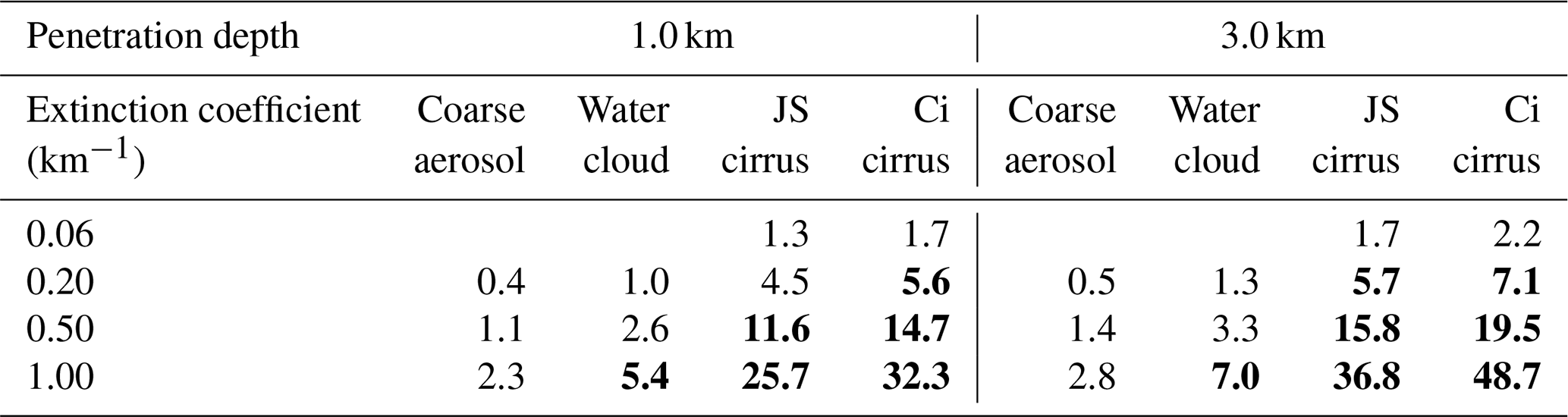
The applicability of the single-scattering approximation (SSA) to lidar signals can be assessed on the basis of R_MSto1(d) values. The percentage of the multiple-scattering relative contribution to lidar signals is shown in Tables 2–3. Those values were computed using corresponding V(d,a) functions, which allow random-noise smoothing. We recall that random noise is inherent in MC simulations. The sample size of our modelling is already very large, i.e. at the limit of our computing capacities.

In the subsequent discussion, we assume a 5 % threshold for the R_MSto1(d) values to consider the single-scattering approximation to be acceptable. It follows from EARLINET (European Aerosol Research Lidar Network) instrument intercomparison campaigns (Fig. 4b in Wandinger et al., 2016) that the relative deviation of the lidar signals (λ=0.532 µm) from the common reference is mostly within ±3 %. In our opinion, an MS contribution lower than 5 % could hardly be detected in such conditions. It should be underlined that the results of this work are presented so that an interested reader can use other threshold values to assess whether the single-scattering approximation is acceptable in view of measurement errors in a specific lidar.

The values exceeding that threshold are highlighted by the bold font in Tables 2–3. In our opinion, the most important outcome is the fact that the SSA has to be rejected in the cases of cirrus clouds when the RFOV is 1.0 mrad (see Table 2). Even with ε_p=0.06 km⁻¹ and d=1.0 km the multiple-scattering contribution is about 4 %. As for the RFOV 0.25 mrad (see Table 3), the SSA is acceptable for the cirrus clouds only with ε_p=0.1 km⁻¹ or lower. Actually, the overwhelming majority of the values in Table 2 are beyond the threshold. Thus, a RFOV of 1.0 mrad cannot be recommended when the distance to a layer of particles is about 8 km or higher. The SSA is acceptable for the coarse aerosol when the RFOV is 0.25 mrad (see Table 3). That conclusion holds true for the fine-mode aerosols (they have lower values of the effective diameter). As for the water cloud, the SSA is acceptable when ε_p≲0.5 km⁻¹, and the RFOV is 0.25 mrad.

As it was mentioned above, the majority of works take into account multiple scattering employing one of the possible multiple-scattering functions (MSF). Moreover, the simplified version η_MS(d)=const of the MSF η_MS(d) is frequently employed in inverse problems. That is the reason why we provide η_MS(d) computed on the basis of our MC simulations (see Eq. 7 and details in Appendix B).

As for the MSF η_MS(d) in Fig. 4, the values of η_MS(d) are so close within each panel that the green points (ε_p(d)=0.2 km⁻¹) sometimes totally cover other colours. In other words, the impact of multiple scattering has the same growth rate when plotted as a function of the in-cloud depth, and the extinction coefficient is quite low ε_p(d)≤1.0 km⁻¹. Each type of particle, of course, has its own growth rate. That property is not valid when the impact of multiple scattering is quite high (see Sect. 6 below).

Generally, there is much in common between all curves η_MS(d). Moreover, such kinds of curves can be found in the literature. For example, the MSF η_MS(d) of the cirrus clouds in Fig. 4g–h are similar to the curves in Fig. 14 of the work by Platt (1981); the discrepancy between the values is most likely due to a difference in phase function properties within the forward-diffraction peak. Generally, the multiple-scattering functions η_MS(d) in Figs. 4, 6, and 8 reveal the same property at the layer near end, i.e. η_MS(d)<1. That result is in total agreement with the theory (see Appendix A2 below).

It is seen in Fig. 4 that η_MS(d) is a nonlinear function. In our opinion, η_MS(d)=const is a rough approximation, while lidar signals are recorded in the usual operational conditions. Its only justification is that it is easily adapted to a solution of an inverse problem. Generally, the solution should be biased, and the level of consequent errors depends on a specific algorithm used to solve the inverse problem. A study of biases can be performed using the results of this work, i.e. the V(d,a) function along with the values of the parameters a.

As expected, our simulations confirm general properties of the multiple-scattering effect on lidar signals that can be found in the literature (see e.g. Eloranta, 1998). Namely, the effect of multiple scattering as well as the relative contribution of the third and higher orders of scattering increase with increased extinction coefficient, in-cloud distance, and receiver field of view. The proportion of light scattered within very small angles, that is, within the forward-diffraction peak (see the inset in Fig. 1), is of upmost importance. That proportion is characterized by the angular width θ_d of the diffraction peak in the work by Eloranta (1998). In contrast, the asymmetry parameter is of little significance for multiple-scattering effects on lidar signals recorded in the UOCs. For instance, the asymmetry-parameter values of the coarse aerosol and the cirrus clouds differ little (see Table 1), whereas there are fundamental differences in the multiple scattering. And, in our opinion, the angle θ_max is more appropriate than θ_d for use as one of the parameters that govern the effect of multiple scattering on lidar signals.

The same kind of study was done in view of the double-scattering contribution. The main conclusion is that the empirical model fits well with the functions R_2to1(d). A representative example can be seen in Fig. S1 of the Supplement.

5.2 Airborne lidar

All but one simulation condition, that is, the input data from the foregoing subsection, were used in our MC simulations for the airborne lidar. Namely, we are dealing with the coaxial zenith-looking lidar that is at an altitude of 7 km, and the distance to the cloud base is 1 km. We recall that the results of Sect. 5 are presented so that they remain unaltered when the lidar pointing angle and/or the layer altitude vary provided that the distance to the cloud base or border remains unchanged.

Figure 5 Multiple-scattering contributions R_MSto1 to lidar signals. Points – MC simulations, black lines – fitting with the empirical model. The full RFOV is 1.0 mrad (a–d) and 0.25 mrad (e–h). Coarse aerosol (a, e), water cloud (b, f), JS cirrus (c, g), Ci cirrus (d, h). The extinction coefficient is 1.0 km⁻¹ (blue points), 0.5 km⁻¹ (red points), 0.2 km⁻¹ (green points), and 0.06 km⁻¹ (purple points). The distance to the cloud base is 1 km.

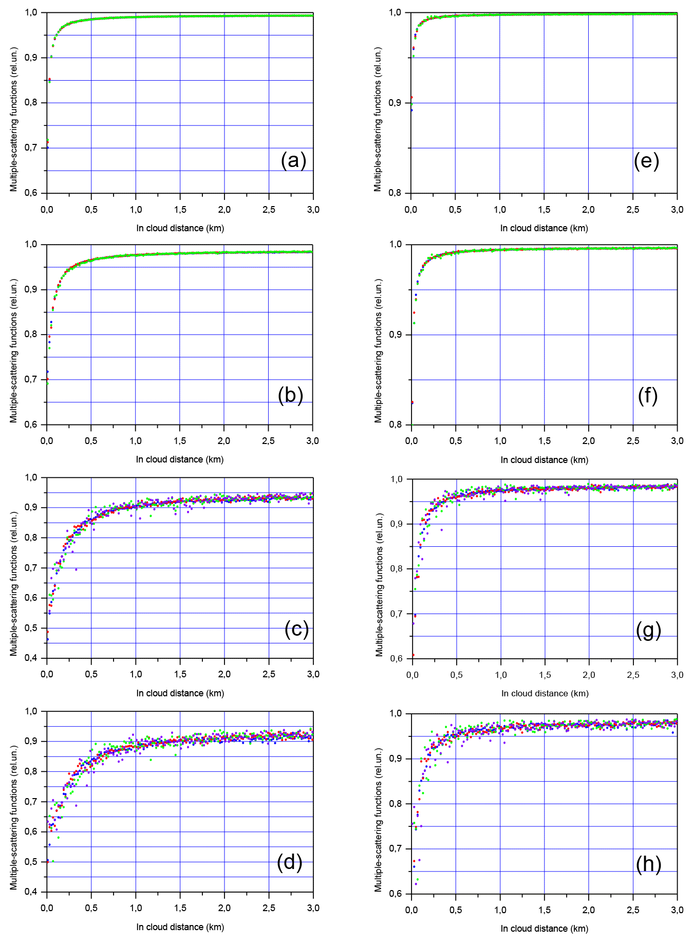
Figure 6 MC simulations of multiple-scattering functions η_MS(d). The full RFOV is 1.0 mrad (a–d) and 0.25 mrad (e–h). Coarse aerosol (a, e), water cloud (b, f), JS cirrus (c, g), Ci cirrus (d, h). The extinction coefficient is 1.0 km⁻¹ (blue points), 0.5 km⁻¹ (red points), 0.2 km⁻¹ (green points), and 0.06 km⁻¹ (purple points). The distance to the cloud base is 1 km.

As in Sect. 5.1, the results of our MC simulations are reported in terms of the ratios R_MSto1(d) and MSF η_MS(d) (Figs. 5 and 6, respectively). Again, the same type of notation was used in both figures. The left-hand column corresponds to the full RFOV of the lidar 1.0 mrad; the right-hand column corresponds to the full RFOV of 0.25 mrad. Blue, red, green, and purple points show the MC simulation results obtained with the extinction coefficient 1.0, 0.5, 0.2, and 0.06 km⁻¹, respectively. The black curves in Fig. 5 represent the fitting results; each curve corresponds to its own set of points R_MSto1(d). (The corresponding values of the parameters $\mathbf{a}=\left\{a_{\mathrm{1}},a_{\mathrm{2}},a_{\mathrm{3}}\right\}$ are given in Tables S3 and S4 of the Supplement.) The effect of multiple scattering is much lower when compared to the ground-based lidar. That does not affect the quality of fitting with the V(d,a) function.

Table 4 Multiple-scattering contribution to lidar signals in per cent (%) of the single scattering. The distance to the cloud base is 1 km; the lidar RFOV is 1.0 mrad. Values exceeding 5 % threshold are in bold font.

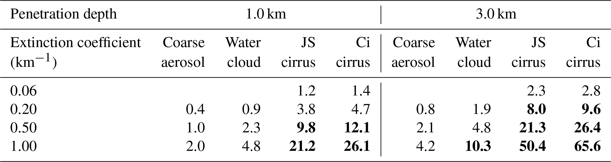
Table 5 Multiple-scattering contribution to lidar signals in per cent (%) of the single scattering. The distance to the cloud base is 1 km; the lidar RFOV is 0.25 mrad. Values exceeding 5 % threshold are in bold font.

The percentage of the multiple-scattering relative contribution to lidar signals is shown in Tables 4–5. Those values were computed using corresponding V(d,a) functions, which allow random-noise smoothing. As expected, the multiple-scattering contribution decreased as the distance to the cloud base decreased. More specifically, the ratio R_MSto1 decreased by a factor of 2.7 to 4.8 when the distance to the cloud base decreased by a factor of 8. The reduction is more significant for the penetration depth of 1 km. It is around 4.5 times for the full RFOV of 0.25 mrad. When the full RFOV is 1.0 mrad, the reduction is around 4.5 times for the coarse aerosol and the water cloud and around 3.5 times for the cirrus clouds. The reduction is clearly lower, i.e. around 3 times, for a penetration depth of 3 km.

Again, we assume a 5 % threshold for the R_MSto1(d) values to consider the single-scattering approximation to be acceptable. The values exceeding that threshold are highlighted by the bold font in Tables 4–5. Special attention should be given to the fact that, in the cases of the cirrus clouds, the effect of multiple scattering is at levels below the threshold only at quite low values of the extinction coefficient.

Again, we provide η_MS(d) computed on the basis of our MC simulations (see Eq. 7 and details in Appendix B). We can conclude again that η_MS(d) is a nonlinear function, and η_MS(d)=const is a rough approximation, while lidar signals are recorded in the usual operational conditions.

The general features of the ratios R_MSto1(d) discussed at the end of in Sect. 5.1 hold true for the airborne lidar.

5.3 Estimation of MS magnitude in other cases

These work data are limited to a set of cases because MC simulations are time-consuming. Some ideas about dependence of the MS relative contribution R_MSto1 on the lidar-configuration parameters and on the particle characteristics can be obtained from an analysis of Eq. (11) of the work by Eloranta (1998). That equation is very complex, and numerical integration has to be done even when the extinction coefficient is constant. Thus, it is hardly probable that relatively simple estimations of the coefficients $\mathbf{a}=\left\{a_{\mathrm{1}},a_{\mathrm{2}},a_{\mathrm{3}}\right\}$ can be developed directly. In such a situation, it is reasonable to suggest a way to predict some useful characteristics.

The magnitude of MS contribution to lidar signals, i.e. the level of R_MSto1, is of special interest because, for example, it indicates whether the single-scattering approximation can be used in other cases under the usual operational conditions. Analysis of the literature (see e.g. Eloranta, 1998) suggests that there exist key parameters governing MS contribution, namely, the receiver field of view RFOV, the distance to the cloud near edge h_b, the in-cloud distance d, the particle extinction coefficient ε_p, and the angle θ_max. And, as follows from Eq. (14) and seen in Figs. 3 and 5, R_MSto1∼d when the in-cloud distance d exceeds 0.5 km.

The first idea that comes is to search for approximate relationships between R_MSto1 and the key parameters for the range d>0.5. Thereupon, those approximate relationships can be used along with the data of Tables 2–4 to estimate the magnitude of MS contribution to lidar signals in cases of interest.

It follows from MC simulations of this work that $R_{\mathrm{MSto}\mathrm{1}}\sim (\mathrm{RFOV}{)}^{k_F}$, $R_{\mathrm{MSto}\mathrm{1}}\sim {\left({\mathit{\epsilon }}_{\mathrm{p}}\right)}^{k_{\mathit{\epsilon }}}$, $R_{\mathrm{MSto}\mathrm{1}}\sim {\left({\mathit{\theta }}_{max}\right)}^{-k_{\mathit{\theta }}}$, $R_{\mathrm{MSto}\mathrm{1}}\sim {\left(h_b\right)}^{k_h}$, and R_MSto1∼d. (We recall that the width θ_max or θ_d of the forward-scattering peak depends on the wavelength and the effective size of particles.) The powers k_F, k_ε, k_θ, and k_h are approximately within the following ranges: $k_F\in \left[\mathrm{0.9},\mathrm{1.1}\right]$, $k_{\mathit{\epsilon }}\in \left[\mathrm{0.6},\mathrm{1.3}\right]$, $k_{\mathit{\theta }}\in \left[\mathrm{0.3},\mathrm{1.1}\right]$, and $k_h\in \left[\mathrm{0.5},\mathrm{0.7}\right]$. The fact that the powers are within some intervals means that there is strong nonlinear interdependence between effects of the key parameters. Therefore, an estimation of the magnitude of MS contribution will be rough even in the UOC.

The effective diameter d_eff of the fine-mode aerosols is lower than d_eff of the coarse mode (see e.g. Dubovik et al., 2006), and the same is true for hydrated-sea-salt aerosol (see e.g. Masonis et al., 2003). Consequently, the forward-scattering peaks of those aerosols are larger. Therefore, it is safe to say that the coarse-aerosol data of Tables 2–4 can be used as the upper bounds for fine-mode aerosols and for hydrated-sea-salt aerosol. The mean values of the effective diameter of marine and continental low-level stratiform clouds are 19.2 and 10.8 µm, respectively (Miles et al., 2000). Thus, the water-cloud data of Tables 2–4 can be useful when ε_p≤1.0 km⁻¹. (The cases of high values of the particle extinction coefficient are addressed below.)

In support of the approach above we obtained the following results. Optical characteristics of sea-salt aerosol were computed at a wavelength of 0.532 µm. The size distribution of particles was assumed to be log-normal with a mean radius of 2 µm, standard deviation of 0.6 µm, and d_eff = 4.75 µm, that is, the same as for the coarse mode. We used the mixture of spheroids with the distribution of axis ratios within the range [0.9129, 1.0954], and the real and imaginary parts of the refractive index were 1.40 and 0.0006, respectively (Masonis et al., 2003). The obtained phase function has ${\mathit{\theta }}_{max}=\mathrm{2.37}$^∘, which is larger than θ_max of the coarse mode due to the changes in the refractive index and the shape of particles. Assuming that $R_{\mathrm{MSto}\mathrm{1}}\sim {\left({\mathit{\theta }}_{max}\right)}^{-\mathrm{1}}$, we used Tables 2 and 4 to estimate the MS magnitude for the cases ε_p=1.0 km⁻¹, RFOV 1.0 mrad, and distances to the sea-salt aerosol layer of 1 and 8 km. The estimations of the approach above lead to values of 3.8 % and 11.6 %, respectively, at an in-cloud distance of 3 km. As the reference, MC simulations gave 3.7 % and 11.0 % for the same cases.

It is well known that the phase function of ice particles depends not only on the effective size but also on particle habit (see e.g. Yang et al., 2013) and roughness of particle surface (see e.g. Shcherbakov et al., 2006). The data library (Yang et al., 2013) provides reliable scattering, absorption, and polarization properties of ice particles in large spectral and size ranges, 11 ice crystal habits, and 3 surface roughness conditions (i.e. smooth, moderately roughened, and severely roughened). The data library provides means to obtain the angle θ_max and estimate MS magnitude using Tables 2–4. Broadly speaking, large differences with the results of this work are hardly expected for other habits of ice particles provided that the surface of the facets is severely roughened. When the surface of the facets is smooth – that is, the halo features are present in a phase function – a higher or much higher MS magnitude could be expected because much more energy is scattered within very small forward angles even in the case of an ensemble of randomly oriented particles (Yang et al., 2013).

6 High impact of multiple scattering

6.1 Spaceborne lidars

6.1.1 Moderate and small extinction coefficient

Figures 7 and 8 show examples of the multiple-scattering effect on signals of spaceborne lidars, i.e. the ratios R_MSto1(d) and the MSF η_MS(d), respectively. The MS impact is high; accordingly, we use log-linear graphs in Fig. 7. As previously, we maintain the same type of notation in both figures. The left-hand column corresponds to the CALIOP configuration; the right-hand column corresponds to the ATLID configuration. Blue, red, green, and purple points show the MC simulation results obtained with the extinction coefficient 1.0, 0.5, 0.2, and 0.06 km⁻¹, respectively. The black curves represent the fitting results; each curve corresponds to its own set of points R_MSto1(d).

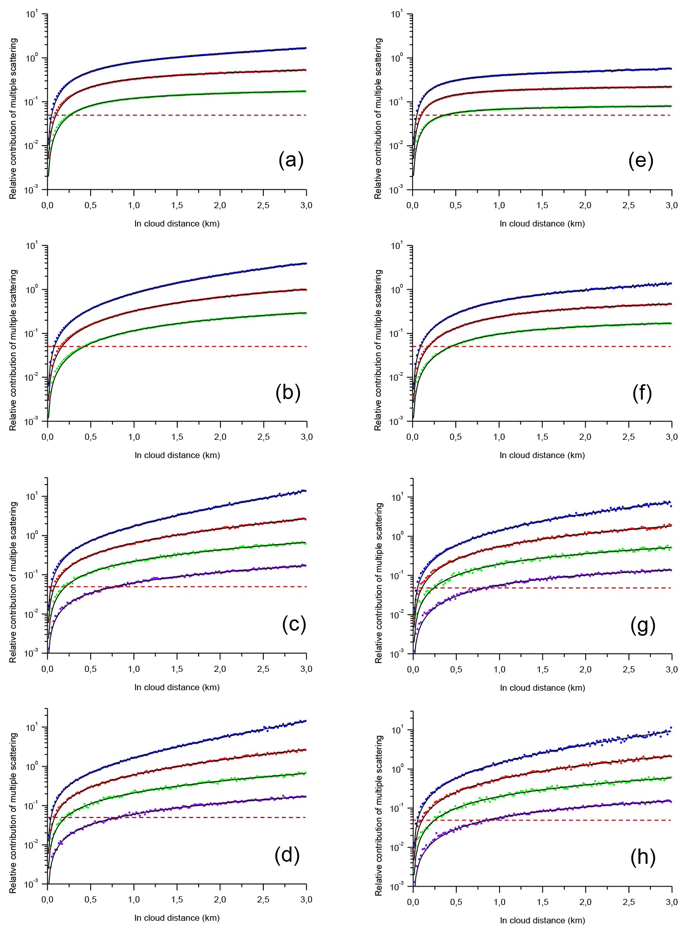
Figure 7 Multiple-scattering contributions R_MSto1 to lidar signals. Points – MC simulations, black lines – fitting with the empirical model. The CALIOP configuration (a–d) and the ATLID configuration (e–h). Coarse aerosol (a, e), water cloud (b, f), JS cirrus (c, g), Ci cirrus (d, h). The extinction coefficient is 1.0 km⁻¹ (blue points), 0.5 km⁻¹ (red points), 0.2 km⁻¹ (green points), and 0.06 km⁻¹ (purple points). The dashed red lines indicate the 5 % threshold.

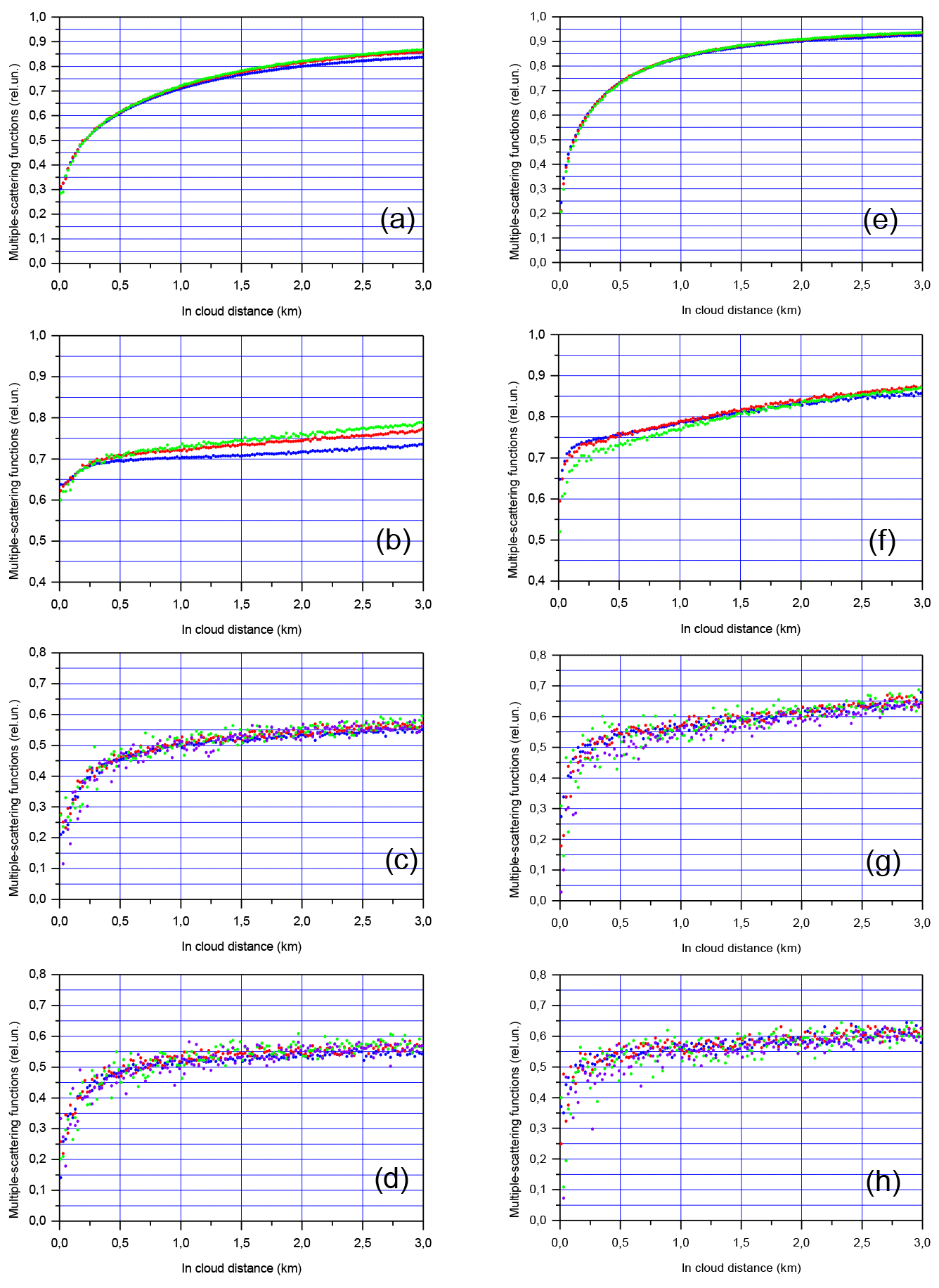
Figure 8 MC simulations of multiple-scattering functions η_MS(d). The CALIOP configuration (a–d) and the ATLID configuration (e–h). Coarse aerosol (a, e), water cloud (b, f), JS cirrus (c, g), Ci cirrus (d, h). The extinction coefficient is 1.0 km⁻¹ (blue points), 0.5 km⁻¹ (red points), 0.2 km⁻¹ (green points), and 0.06 km⁻¹ (purple points).

The features of all ratios R_MSto1(d) in Fig. 7 have much in common despite the large differences in scattering matrixes of particles. Such kinds of figures can be found in the literature (see e.g. Fig. 2 in Winker, 2003). Moreover, we performed MC simulations in the conditions of Fig. 4 (the second panel of the lower row) of the work by Wang et al. (2021). That is, a water cloud has an extinction coefficient of 13.33 km⁻¹, the lidar transmitter has a wavelength of 0.532 µm, the full RFOV is 0.10 mrad, and the distance from the lidar to the cloud is 703.7 km. The points of our simulated ratio R_MSto1(d) superimpose almost perfectly on the corresponding curve of the work by Wang et al. (2021). The MSF η_MS(d) of the coarse aerosol in Fig. 7a and e resemble the curves in Fig. 3 of the work by Winker (2003). The difference in the values can be due to the fact that the phase function of this work (see Fig. 1) has more pronounced forward scattering. There is a discordance at the near end of cirrus clouds between the MSF η_MS(d) in Figs. 8c–d and 7 of the work by Winker (2003). It seems that the discordance results from the 5-times-finer spatial resolution used in our MC simulations.

It is seen that our empirical model Eq. (10) fits well with the MC data in Fig. 7. The values of the free parameters $\mathbf{a}=\left\{a_{\mathrm{1}},a_{\mathrm{2}},a_{\mathrm{3}}\right\}$ were computed using the ordinary least squares method. (The corresponding values of the parameters $\mathbf{a}=\left\{a_{\mathrm{1}},a_{\mathrm{2}},a_{\mathrm{3}}\right\}$ are given in Tables S5 and S6 of the Supplement.) The dashed red line indicates the 5 % threshold for the multiple-scattering relative contribution R_MSto1(d). In our opinion, the contribution below 5 % is so exceptional that the single-scattering approximation should never be applied to data of spaceborne lidars.

As is expected, the MSFs η_MS(d) in the panels of Fig. 8 have lower values compared to the corresponding panels in Fig. 4. This confirms that the MS effect is much more pronounced throughout all in-cloud ranges. Again, we can underline that η_MS(d)=const is only a rough approximation. At the same time, the approximation Eq. (19) seems to be valid within a quite large range of penetration depths. In addition, there are changes in MSF behaviour. Unlike in the cases of Sect. 5, η_MS(d) depends on the extinction coefficient (see e.g. Fig. 9a–b).

The general features of the ratios R_MSto1(d) discussed at the end of Sect. 5.1 hold true for spaceborne lidars. In particular, the angle θ_max is more appropriate for use as one of the parameters that govern the effect of multiple scattering on lidar signals.

6.1.2 High extinction coefficient of water clouds

In the foregoing subsection, we studied the cases when the values of the extinction coefficient were quite small (≤1.0 km⁻¹). Such a limitation does not conform to warm-cloud properties. Therefore, we performed MC simulation with higher values of ε_p. We kept most of the simulation conditions of the previous section, that is, the CALIOP configuration; the water cloud is within the altitude range of 8–11 km. We employed the refined spatial resolution of 5 m, and 50 orders of scattering were taken into account.

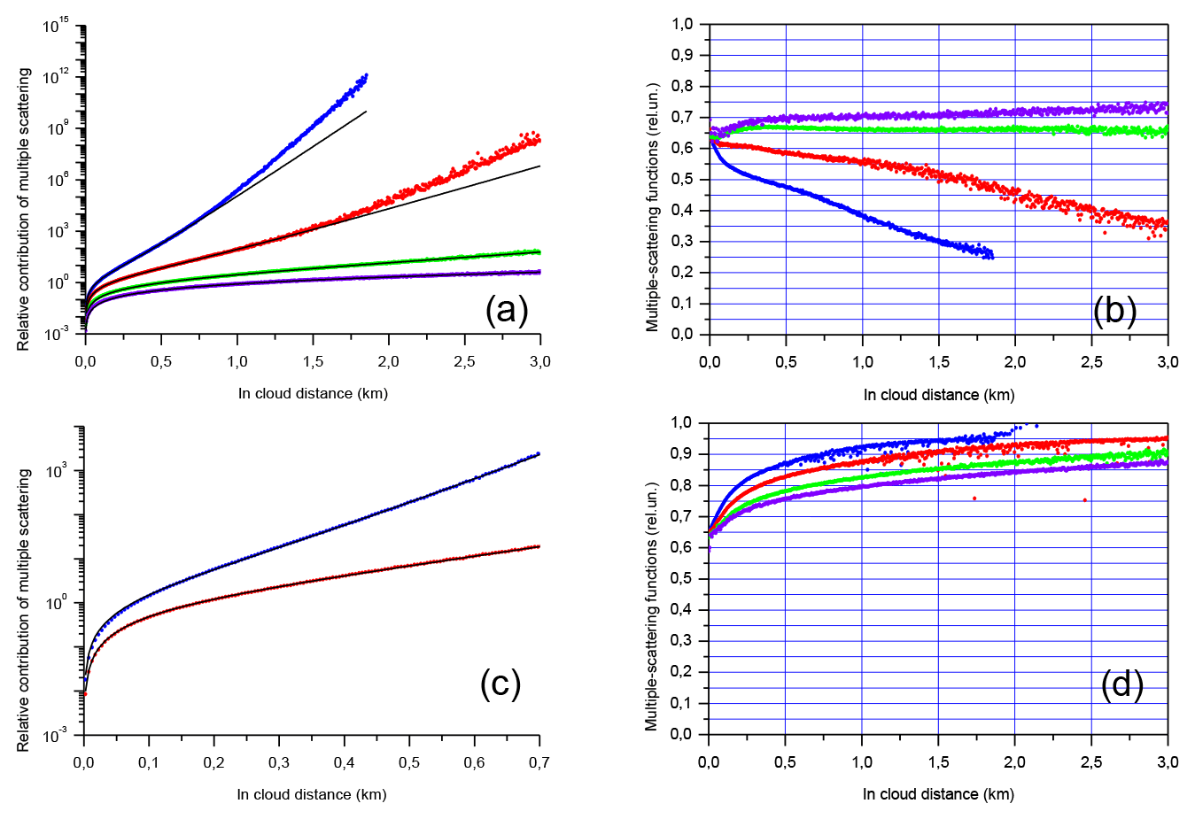
Figure 9 Multiple-scattering contributions R_MSto1 to lidar signals (a). Points – MC simulations, black lines – fitting with the empirical model. Panel (c) is the same as panel (a) but for the shorter in-cloud range, and only two values of the extinction coefficient are shown. Multiple-scattering functions η_MS(d) for multiple scattering (b) and double scattering (d). The extinction coefficient is 10.0 km⁻¹ (blue points), 5.0 km⁻¹ (red points), 2.0 km⁻¹ (green points), and 1.0 km⁻¹ (purple points).

Figure 9a and b show examples of the multiple-scattering effect on lidar signals, i.e. the ratios R_MSto1(d) and the MSF η_MS(d), respectively. In order to evidence the quality of the fitting, we provide R_MSto1(d) within the range d∈ 0–0.7 km in Fig. 9c. The MSFs η₂(d) of the double scattering are shown in Fig. 9d. It was computed according to Eq. (7), while only two orders of scattering were taken into account. As previously, we maintain the same type of notations in all figures. Blue, red, green, and purple points show the MC simulation results obtained with the extinction coefficient 10.0, 5.0, 2.0, and 1.0 km⁻¹, respectively. The case ε_p=10.0 km⁻¹ is shown up to a penetration depth of 1.84 km because the statistical significance of the MC data became extremely low beyond that distance. The black curves represent the fitting results; each curve corresponds to its own set of points R_MSto1(d). According to the conclusion of Sect. 3, only the data that correspond to the penetration optical depth ≤ 7.0 were taken into account for fitting. It is seen in Fig. 9a and c that there is good agreement between the MC data and the empirical model Eq. (10) when that condition is satisfied. The blue and red points begin to deviate from the corresponding fitting curves at τ_p(d)=7.0. It should be underlined that the same property is observed for two profoundly different configurations, i.e. CALIOP Fig. 9a and MUSCLE Fig. 2a.

It is instructive to observe the behaviour of the MSF η_MS(d) in Figs. 8b and 9b. The MSF slightly increases with the in-cloud distance when ε_p<2.0 km⁻¹, it is almost constant at ε_p=2.0 km⁻¹, and it decreases when ε_p>2.0 km⁻¹. In other words, the impact of multiple scattering has the growth rate lower than, equal to, and higher than the exponential, respectively. All that leads to the large variation in the MSF values in Fig. 9b. As for the double-scattering MSF η₂(d) in Fig. 9d, it always increases. The higher the extinction coefficient ε_p, the higher η₂(d) is, or to put it differently, the lower the part of the double-scattering is. We note in passing that Fig. 9b and d lead to the conclusion that the MSF η_MS(d) will be overestimated if the number of scattering orders taken into account in MC simulations is deficient. To conclude this subsection, we underline that our empirical model has successfully fitted the MC data despite the profound changes in the MS growth rate. (The corresponding values of the parameters $\mathbf{a}=\left\{a_{\mathrm{1}},a_{\mathrm{2}},a_{\mathrm{3}}\right\}$ are given in Table S7 of the Supplement.)

6.2 Wide field of view

The multiple-field-of-view techniques already have more than 4 decades of history in lidar measurements (see e.g. Allen and Platt, 1977; Bissonnette et al., 2005; and Jimenez et al., 2020). Multiple-scattering impact is favoured by increasing RFOV. Therefore, it is interesting to evaluate the performance of the empirical model against MC simulations when the RFOV is quite wide. The simulations were performed under the same conditions as in Sect. 5.1; that is, for the ground-based lidars, the water cloud is within the altitude range of 8–11 km, the extinction coefficient is 1.0 km⁻¹, and 40 orders of scattering were taken into account.

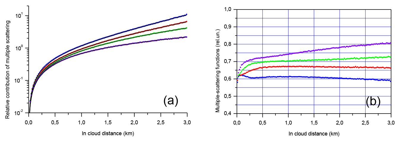
Figure 10 Multiple-scattering contributions R_MSto1 to lidar signals (a). Points – MC simulations, black lines – fitting with the empirical model. Multiple-scattering functions η_MS(d) (b). The RFOV is of 50 mrad (blue points), 20 mrad (red points), 10 mrad (green points), and 5 mrad (purple points). The distance to the cloud base is 8 km.

Figure 10a and b show examples of the multiple-scattering effect on lidar signals, i.e. the ratios R_MSto1(d) and the MSF η_MS(d), respectively. As previously, we maintain the same type of notation in all figures. Blue, red, green, and purple points show the MC simulation results obtained with RFOVs of 50, 20, 10, and 5 mrad, respectively. (The cases of an RFOV of 0.25 and 1 mrad are shown in Figs. 3f and b and 4f and b.) The black curves represent the fitting results; each curve corresponds to its own set of points R_MSto1(d). It is seen in Fig. 10a that there is good agreement between the MC data and the empirical model Eq. (10). (The corresponding values of the parameters $\mathbf{a}=\left\{a_{\mathrm{1}},a_{\mathrm{2}},a_{\mathrm{3}}\right\}$ are given in Table S8 of the Supplement.) As in the cases of high extinction coefficient (see Fig. 9b), there are profound changes in behaviour of the MSF η_MS(d) when the RFOV increases. All MSFs η_MS(d) increase with the in-cloud distance at the near end. The MSFs continue increasing for RFOVs of 5 and 10 mrad; i.e. the impact of multiple scattering has a growth rate lower than the exponential. In contrast, the MSFs start decreasing at an in-cloud distance of about 1 km for RFOVs of 20 and 50 mrad; i.e. the impact of multiple scattering has a growth rate higher than the exponential. All that leads to the large variation in the MSF values in Fig. 10b.

7 Conclusions and discussion

We performed extensive Monte Carlo simulations of single-wavelength lidar signals from a plane-parallel homogeneous layer of atmospheric particles. The simulations have taken into consideration four types of configurations (the ground based, the airborne, the CALIOP, and the ATLID) and four types of particles (coarse aerosol, water cloud, jet-stream cirrus, and cirrus), which have large difference in microphysical and optical properties. Most of the simulations were performed with a spatial resolution of 20 m and a particle extinction coefficient between 0.06 and 1.0 km⁻¹. The resolution was 5 m for high values of ε_p (up to 10.0 km⁻¹). The majority of the simulations for ground-based and airborne lidars were performed at two values of the receiver field of view: 0.25 and 1.0 mrad. The effect of the width of the RFOV was studied for values up to 50 mrad. In order to assure good statistical quality of our Monte Carlo modelling, each signal was simulated with 4×10¹⁰ photons emitted by the lidar (with 4×10¹¹ photons for the cirrus clouds having ε_p=0.06 km⁻¹).

Such a large set of configurations and particle characteristics covers a broad range of the multiple-scattering (MS) relative contribution to lidar signals: from lower than 5 % to a factor of several thousand. Despite the broad range of variations, all MS relative contributions have the same general behaviour as a function of the in-cloud penetration depth when plotted as a log-linear graph. At the near end, the function R_MSto1(d) is linearly proportional to the in-cloud distance d. Then, the curve bends to the right and continues to increase at the same rate within a quite large interval. Such common behaviour enabled us to propose the empirical model, which has demonstrated very good quality of MC data fitting for all considered cases. We have not encountered any exception despite profound changes in the MS growth rate at high values of the extinction coefficient or wide RFOVs. When R² is used to estimate goodness of fit (see e.g. Motulsky and Christopoulos, 2004) to the MC data, all fittings in Figs. 7, 9, and 10 as well as the overwhelming majority in Figs. 3 and 5 have R²>0.99. Lower values of R² were obtained for the cases of cirrus clouds in the usual operational conditions.

The fact that the MS relative contribution can be fitted by a simple function for a large set of lidar configurations and particle characteristics is of importance by itself. It provides a new perspective on the problem of the radiative transfer related to lidar and radar measurements.

Special attention was given to the usual operational conditions; i.e. when the distance from a lidar to a layer of particles is lower than 15 km, the RFOV ≤ 1 mrad, the emitter field of view (EFOV) ≤ 0.2 mrad, EFOV ≪ RFOV, and the extinction coefficient ε≤1 km⁻¹. We assumed a 5 % threshold for the MS impact to consider the single-scattering approximation to be acceptable. It follows from our Monte Carlo simulations that the multiple-scattering effects cannot be neglected when the distance to a layer of particles is about 8 km or higher, and the full RFOV is 1.0 mrad. As for the full RFOV of 0.25 mrad, the single-scattering approximation is acceptable for aerosols (ε_p≲1.0 km⁻¹), water clouds (ε_p≲0.5 km⁻¹), and cirrus clouds (ε_p≤0.1 km⁻¹). When the distance to a layer of particles is 1 km, the single-scattering approximation is acceptable for aerosols and water clouds (ε_p≲1.0 km⁻¹, both RFOV = 0.25 mrad and RFOV = 1 mrad). As for cirrus clouds, the effect of multiple scattering cannot be neglected even at such a low distance when ε_p≳0.5 km⁻¹.

As for spaceborne lidars, the contribution of multiple scattering below 5 % is so exceptional that the single-scattering approximation should never be applied to data of such lidars.

Our simulations confirm general properties of the multiple-scattering effect on lidar signals that can be found in the literature. Namely, the MS impact as well as the relative contribution of the third and higher orders of scattering increases with increased extinction coefficient, in-cloud distance, and receiver field of view. The proportion of light scattered within forward angles is of upmost importance. Our results suggest that the angle θ_max is more appropriate to characterize that proportion, i.e. for use as one of the parameters that govern the effect of multiple scattering on lidar signals.

We computed the multiple-scattering function η_MS(d) on the basis of our MC data. If follows that η_MS(d) is a nonlinear function. The assumption η_MS(d)=const is a rough approximation. It is equivalent to the assumption that the impact of multiple scattering has an exponential growth rate as a function of the in-cloud optical depth. Generally, this is not the case, especially at the cloud near end. Moreover, the growth rate as well as the MSF η_MS(d) depends on the particle extinction coefficient and/or the RFOV of all other parameters being the same. In our opinion, the only justification of the assumption η_MS(d)=const is that it is easily adapted to a solution of an inverse problem.

Despite the fact that this work is limited to the cases of homogeneous layers, we can propose two immediate application of our results. The empirical model along with the parameters $\mathbf{a}=\left\{a_{\mathrm{1}},a_{\mathrm{2}},a_{\mathrm{3}}\right\}$ given in tables of the Supplement provides a fast and accurate way to simulate lidar signals in multiple-scattering conditions for a large range of experimental situations. Thus, an interested reader can obtain a set of accurate data without performing time-consuming Monte Carlo simulations.

The first application is that the set of data is used to compute profiles of apparent backscatter, which are employed to test inverse-problem algorithms. Therefore, a developer of an inverse algorithm can see its quality.

The second application is the following. As stated in the introduction, the accuracy level and the applicability bounds of the approximate models still need to be rigorously evaluated. Such an evaluation should be done in terms of the MS relative contribution, not in terms of apparent backscatter, because a model is devoted to simulating the MS effect. The evaluation should be done for a large range of experimental situations. Thus, the results of our work provide an easy way to begin the evaluation.

This work should be considered to be the starting stage of the model development if needs of a practitioner are taken into account, especially when an inverse problem is to be solved (see e.g. Voudouri et al., 2020). The next two stages have to be fulfilled: (i) development of an approach that predicts $\mathbf{a}=\left\{a_{\mathrm{1}},a_{\mathrm{2}},a_{\mathrm{3}}\right\}$ values only on the basis of the lidar configuration and particle characteristics and (ii) generalization of the V(d,a) function in the case of varying profiles of the extinction coefficient.

It seems that the function V(d,a) is able to capture the fundamental properties of radiative transfer in the conditions of lidar or radar sounding. Our preliminary results (not shown here) suggest that the empirical model can be fruitful when multiple-scattering effects are taken into account in measurements with radars, Raman lidar, and high-spectral-resolution lidars as well as in profiles of linear and circular depolarization ratios. Detailed study of empirical-model capacity in those cases is a subject of our future work.

Appendix A: Multiple-scattering functions

A1 Definitions and relationships

The utility of a multiple-scattering function (MSF) consists of the possibility of considering effects of multiple scattering while dealing with equations similar to the single-scattering lidar Eq. (1). In what follows, the MSFs are written as functions only of the distance h. It should be keep in mind that they depend on particle characteristics and lidar parameters. The notations of Sect. 3 are used in this Appendix, and some relationships of Sect. 3 are repeated for convenience.

Several approaches to define a MSF can be found in the literature. Similarly to the transport approximation of the radiative transfer theory (see e.g. chap. 17 of Davison, 1957), the constant factor η was proposed by Platt (1973) to account for “secondary scattering or higher order processes”. In the work by Platt (1979), η (in our notations the MSF η_MS(h)) was defined as the factor that multiplies the optical depth, has a value less than unity, and may vary with altitude. According to the notations used in the work by Winker (2003), lidar signals that have been corrected for the offset and instrumental factors can be written as

$$\begin{array}{}\text{(A1)}& \begin{array}{rl}{S}_{\mathrm{MS}}\left(h\right)& =\left[{\mathit{\beta }}_{\mathrm{p}}\left(h\right)+{\mathit{\beta }}_{\mathrm{m}}\left(h\right)\right]\cdot T_{\mathrm{m}}^{\mathrm{2}}\left(h\right)\\ & \cdot \exp ⌈-\mathrm{2}{\mathit{\eta }}_{\mathrm{MS}}\left(h\right){\mathit{\tau }}_{\mathrm{p}}\left(h_b,h\right)⌉,\end{array}\end{array}$$

where ${\mathit{\tau }}_{\mathrm{p}}\left(h_b,h\right)={\int }_{h_b}^h{\mathit{\epsilon }}_{\mathrm{p}}\left(h^{\prime }\right)\mathrm{d}{h}^{\prime }$ is the in-cloud optical depth, and ε_p(h) is the extinction coefficient of particles.

Another multiple-scattering function F_MS(h) was proposed in the work by Kunkel and Weinman (1976) as “a factor, which corrects the extinction coefficient”. According to the work by Wandinger (1998), where F_MS(h) was employed with explicit separation of molecular and particle characteristics, lidar signal can be written in the form

$$\begin{array}{}\text{(A2)}& \begin{array}{rl}{S}_{\mathrm{MS}}\left(h\right)& =\left[{\mathit{\beta }}_{\mathrm{p}}\left(h\right)+{\mathit{\beta }}_{\mathrm{m}}\left(h\right)\right]\cdot T_{\mathrm{m}}^{\mathrm{2}}\left(h\right)\\ & \cdot \exp \left\{-\mathrm{2}\underset{h_b}{\overset{h}{\int }}\left[\mathrm{1}-F_{\mathrm{MS}}\left(h^{\prime }\right)\right]{\mathit{\epsilon }}_{\mathrm{p}}\left(h^{\prime }\right)\mathrm{d}{h}^{\prime }\right\}.\end{array}\end{array}$$

It is reasonable that the MSFs appeared in Eqs. (A1)–(A2) in the terms related to the particle extinction. The phase function of particles has a sharp forward peak (see examples in Fig. 1). The forward-scattered light remains within the RFOV. Thus, the corresponding optical depth is lower than it has to be in the case of the single scattering. In contrast, the molecular phase function is smooth. Therefore, a negligibly small fraction of scattered photons remain within the RFOV. We performed MC simulations with the aim to estimate the contribution of multiple scattering to lidar signals from the standard molecular atmosphere. We considered the same lidar parameters as in Sect. 5.1, i.e. the ground-based lidar with a full RFOV of 1.0 mrad. It follows from our results that the mean value 〈R_MSto1(h)〉 of the molecular contribution was about $\mathrm{4}\times {\mathrm{10}}^{-\mathrm{5}}$ for the layer within the altitude range of 8–11 km.

Another way to consider the multiple scattering is used in the automated algorithm of the Atmospheric Radiation Measurement programme's Raman lidar (Thorsen and Fu, 2015); i.e. the MSF (in our notations G_MS(h)) is a factor which corrects the lidar signal of the single-scattering approximation:

$$\begin{array}{}\text{(A3)}& S_{\mathrm{MS}}\left(h\right)=G_{\mathrm{MS}}\left(h\right)\cdot \left[{\mathit{\beta }}_{\mathrm{p}}\left(h\right)+{\mathit{\beta }}_{\mathrm{m}}\left(h\right)\right]\cdot T_{\mathrm{m}}^{\mathrm{2}}\left(h\right)\cdot T_{\mathrm{p}}^{\mathrm{2}}\left(h\right).\end{array}$$

As a matter of fact, Eq. (A3) is no more than a mathematical expression that provides an easy way to assign the relationship between S_MS(h) and S₁(h). A specific model of multiple scattering appears only when G_MS(h) is given in an explicit form.

It is obvious that

$$\begin{array}{}\text{(A4)}& G_{\mathrm{MS}}\left(h\right)={\displaystyle \frac{S_{\mathrm{MS}}\left(h\right)}{S_{\mathrm{1}}\left(h\right)}}=\mathrm{1}+R_{\mathrm{MSto}\mathrm{1}}\left(h\right),\end{array}$$

and properties of G_MS(h) are seen directly from our result of the numerical simulations in Sects. 5 and 6.

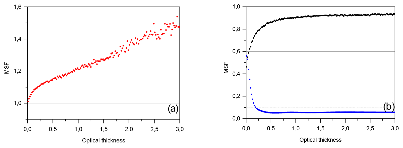
Figure A1 Multiple-scattering functions. (a) Red points G_MS(h), (b) black points η_MS(h) and blue points F_MS(h).

It is a straightforward matter to transform Eqs. (A1) and (A2) into the following forms:

$$\begin{array}{}\text{(A5)}& {\displaystyle }\begin{array}{rl}{S}_{\mathrm{MS}}\left(h\right)& =\left[{\mathit{\beta }}_{\mathrm{p}}\left(h\right)+{\mathit{\beta }}_{\mathrm{m}}\left(h\right)\right]\cdot T_{\mathrm{m}}^{\mathrm{2}}\left(h\right)\cdot T_{\mathrm{p}}^{\mathrm{2}}\left(h\right)\\ & \cdot \exp \left\{\mathrm{2}\left[\mathrm{1}-{\mathit{\eta }}_{\mathrm{MS}}\left(h\right)\right]{\mathit{\tau }}_{\mathrm{p}}\left(h_b,h\right)\right\},\end{array}\text{(A6)}& {\displaystyle }\begin{array}{rl}{S}_{\mathrm{MS}}\left(h\right)& =\left[{\mathit{\beta }}_{\mathrm{p}}\left(h\right)+{\mathit{\beta }}_{\mathrm{m}}\left(h\right)\right]\cdot T_{\mathrm{m}}^{\mathrm{2}}\left(h\right)\cdot T_{\mathrm{p}}^{\mathrm{2}}\left(h\right)\\ & \cdot \exp \left\{\mathrm{2}\underset{h_b}{\overset{h}{\int }}{F}_{\mathrm{MS}}\left(h^{\prime }\right)\cdot {\mathit{\epsilon }}_{\mathrm{p}}\left(h^{\prime }\right)\mathrm{d}{h}^{\prime }\right\},\end{array}\end{array}$$

which lead to the relationships between the multiple-scattering functions. We have chosen G_MS(h) as the known function because MC simulations provide it almost directly.

$$\begin{array}{}\text{(A7)}& {\displaystyle }{\mathit{\eta }}_{\mathrm{MS}}\left(h\right)=\mathrm{1}-{\displaystyle \frac{\mathrm{1}}{\mathrm{2}\cdot {\mathit{\tau }}_{\mathrm{p}}\left(h_b,h\right)}}\cdot \ln \left[G_{\mathrm{MS}}\left(h\right)\right]\text{(A8)}& {\displaystyle }\mathrm{0.5}\cdot \ln \left[G_{\mathrm{MS}}\left(h\right)\right]=\underset{h_b}{\overset{h}{\int }}{F}_{\mathrm{MS}}\left(h^{\prime }\right)\cdot {\mathit{\epsilon }}_{\mathrm{p}}\left(h^{\prime }\right)\mathrm{d}{h}^{\prime }\end{array}$$

Equation (A7) repeats Eq. (8). As for Eq. (A8), it is a first-kind Volterra integral equation. The straight way to deduce F_MS(h) is numerical differentiation. The problem of numerical differentiation is known to be ill-posed in the sense that small perturbations in the function to be differentiated may lead to large errors in the computed derivative.

An example of the multiple-scattering functions is shown in Fig. A1. The MSFs are shown for the case shown in Figs. 5c and 6c; i.e. the homogeneous cirrus cloud is within the altitude h range of 8–11 km, the extinction coefficient is 1.0 km⁻¹, an airborne lidar is at an altitude h=7 km (the distance to the layer base is 1 km), and the full RFOV is 1.0 mrad. Random noise is seen in G_MS(h), which is inherent in MC simulations. The noise level increases with the penetration into the cloud. The random noise in η_MS(h) remains acceptable when Eq. (A7) is used. As for F_MS(h), errors in the computed derivative were excessive even when the smoothing with a quite large sliding window was applied. Therefore, the function shown in Fig. A1b F_MS(h) was computed using the synergy of the range-dependent smoothing with cubic splines and the method of regularization (see details in Shcherbakov, 2007).

Some misleading statements about properties of the MSFs can be found in the literature. Thus, to complete this section, we note the following. The functions η_MS(h) and F_MS(h) cannot be approximated by constant values within a quite large range of the cloud penetration. The function [1−F_MS(h)] should not be confused with η_MS(h). Their physical meaning is different; the former corrects the extinction coefficient ε_p(h), whereas the latter affects the optical depth τ_p(h_b,h). Consequently, the mathematical properties of those functions are different as well.

A2 Features at the cloud near end

Figures 3 and 5 suggest that the multiple-scattering contribution R_MSto1(h) to lidar signals is linearly proportional to τ_p(h_b,h) at the cloud near end. This is in agreement with the double-scattering approximation of lidar equation (see e.g. Samokhvalov, 1979) as well as with the Eloranta model (Eloranta, 1998). The range when the proportionality is valid is rather short. Nevertheless, some key features of the MSFs can be found on the basis of that approximation. It follows from Eq. (A4) that

$$\begin{array}{}\text{(A9)}& G_{\mathrm{MS}}\left(h\right)\approx \mathrm{1}+b\cdot {\mathit{\tau }}_{\mathrm{p}}\left(h_b,h\right),\end{array}$$

where the coefficient b>0 depends on the phase-function properties. It turns out that $b\approx P_{\mathrm{2},\mathit{\pi }}/P_{\mathit{\pi }}$ (see chap. 4 of Eloranta, 1998) if the Eloranta model is used for simulations.

Equations (A7) and (A9) along with the first two terms of the series expansion of the logarithm ln (1+x) lead to the formula

$$\begin{array}{}\text{(A10)}& {\mathit{\eta }}_{\mathrm{MS}}\left(h\right)\approx \mathrm{1}-\mathrm{0.5}b+\mathrm{0.25}{b}^{\mathrm{2}}\cdot {\mathit{\tau }}_{\mathrm{p}}\left(h_b,h\right),\end{array}$$

which is in agreement with Eq. (18). We used the condition of a homogeneous cloud ε_p(h)=const to obtain the approximation of F_MS(h) from Eqs. (A8)–(A9) by the analytical differentiation

$$\begin{array}{}\text{(A11)}& F_{\mathrm{MS}}\left(h\right)\approx {\displaystyle \frac{\mathrm{0.5}b}{\mathrm{1}+b\cdot {\mathit{\tau }}_{\mathrm{p}}\left(h_b,h\right)}}.\end{array}$$

It is instructive to see the MSF values exactly on the cloud near edge, that is, when h→h_b and ${\mathit{\tau }}_{\mathrm{p}}\left(h_b,h\right)\to \mathrm{0}$:

$$\begin{array}{}\text{(A12)}& {\displaystyle }{G}_{\mathrm{MS}}\left(h\right)=\mathrm{1},\text{(A13)}& {\displaystyle }{\mathit{\eta }}_{\mathrm{MS}}\left(h\right)=\mathrm{1}-\mathrm{0.5}b,\text{(A14)}& {\displaystyle }{F}_{\mathrm{MS}}\left(h\right)=\mathrm{0.5}b.\end{array}$$

Intuition suggests that a lidar signal must satisfy the single-scattering lidar Eq. (1) exactly on the cloud near edge, i.e. when h=h_b. That condition and Eq. (A4) impose the value G_MS(h_b)=1, which is in agreement with Eq. (A12).

When the multiple-scattering effect is ignored throughout the range of distances from a lidar, it is enough to assign η_MS(h)=1 in Eq. (A5) or F_MS(h)=0 in Eq. (A6), and both equations are reduced to Eq. (1). A misleading hypothesis η_MS(h_b)=1, which is somewhat based on that fact, can be found in the literature when the multiple scattering is supposed to be taken into account. The hypothesis that η_MS(h_b)=1 is mathematically unjustified, as is the hypothesis that F_MS(h_b)=0. As a matter of fact, the condition S_MS(h_b)=S₁(h_b) does not impose any restriction on values of η_MS(h_b) or F_MS(h_b); it is fulfilled just due to ${\mathit{\tau }}_{\mathrm{p}}\left(h_b,h_b\right)=\mathrm{0}$. In other words, when h=h_b, ${\mathit{\tau }}_{\mathrm{p}}\left(h_b,h_b\right)=\mathrm{0}$, and Eqs. (A5) and (A6) give the same value as Eq. (1) regardless of the values of η_MS(h_b) or F_MS(h_b). Therefore, Eqs. (A13) and (A14) are not in contradiction with the intuition suggestion. At the same time, the additional requirement that the multiple-scattering contribution R_MSto1(h) to lidar signals is linearly proportional to τ_p(h_b,h) at the cloud near edge imposes the restriction on values of η_MS(h_b) and F_MS(h_b) and leads to Eqs. (A13) and (A14).

Appendix B: Range-gate effect

It is seen from Eq. (7) that values of η_MS are very sensitive to chosen values of the optical depth τ_p(h_b,h) at distances close to the cloud base. We recall that MC simulations require integration over the range gate. Thus, the question arises of whether the value of τ_p(h_b,h_i) should be taken at the far end of the ith range gate or somewhere within it. That question can be answered if Eqs. (1)–(2) are thought of as some mathematical relations where the input parameters can be assigned in an easy-to-use form.

We integrated Eqs. (1)–(2) with the step Δh 20 m to obtain profiles S_1,i and S_MS,i for the distances $h_i=i\cdot \mathrm{\Delta }h$, where $i=\mathrm{1},\mathrm{\dots },N$. The step Δh corresponds to the range gate of our MC simulations. The molecular extinction and scattering were neglected. The particulate extinction ε_p and backscatter β_p coefficients as well as η_MS were assigned to be constant within the whole layer. Thus, we studied effects of the exponential functions of Eqs. (1)–(2). The calculations were performed for a large range of ε_p values (1–50 km⁻¹) and η_MS within the range of [0.6,0.99]. The estimated values ${\stackrel{\mathrm{̃}}{\mathit{\eta }}}_{\mathrm{MS},\mathrm{i}}\left(k\right)$ of the MSF were computed as follows.

$$\begin{array}{}\text{(B1)}& \begin{array}{rl}{\stackrel{\mathrm{̃}}{\mathit{\eta }}}_{\mathrm{MS},\mathrm{i}}\left(k\right)& =\mathrm{1}-{\displaystyle \frac{\mathrm{1}}{\mathrm{2}\cdot \left[\mathit{\tau }\left(\mathrm{0},h_{i-\mathrm{1}}\right)+k\cdot \mathit{\epsilon }\cdot \mathrm{\Delta }h\right]}}\\ & \cdot \ln \left[{\displaystyle \frac{S_{\mathrm{MS},\mathrm{i}}}{S_{\mathrm{1},i}}}\right],\end{array}\end{array}$$

where the coefficient k takes values within the range ]0.0,1.0]​,​​​​​​ and $\mathit{\tau }\left(\mathrm{0},h_{\mathrm{0}}\right)=\mathrm{0}$. Equation (B1) corresponds to Eq. (7) with the difference that the value of τ_p(h_b,h_i) can be taken within the ith range gate. The value of τ_p(h_b,h_i) is taken at the far end of the range gate when k=1.

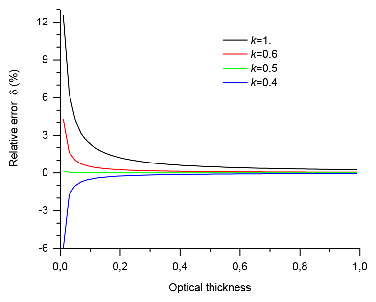
Figure B1 Relative errors as functions of the optical thickness from the layer base and the parameter k. The green line (k=0.5​​​​​​​) and the black line (k=1.0) correspond to the cases when τ(h) is taken in the middle and at the far end, respectively, of the range gate.

A typical example of relative errors ${\mathit{\delta }}_i\left(k\right)=\mathrm{100}\cdot \left({\stackrel{\mathrm{̃}}{\mathit{\eta }}}_{\mathrm{MS},\mathrm{i}}\left(k\right)-{\mathit{\eta }}_{\mathrm{MS}}\right)/{\mathit{\eta }}_{\mathrm{MS}}$ of the estimations is shown in Fig. B1. It is seen that δ_i(k) is close to zero for k=0.5. In contrast, the relative errors are quite high when k=1 and the optical thickness τ_p(h_b,h_i) computed from the layer base are rather small. At the same time, δ_i(k) becomes negligible with increasing optical thickness of the cloud penetration depth. An example of the effect of the coefficient k on the computed values of the MSF η_MS(h_i) is shown in Fig. B2. The black points correspond to the case of Fig. 4b above; that is, h_i was assigned to the middle of the range gate (k=0.5). The red points are the MSF η_MS(h_i) computed using the same MC data but with k=1.0; that is, the values of τ_p(h_b,h_i) were taken at the far end of the range gate. The discrepancies between the curves are obvious. And what is important is that the wrong choice of τ_p(h_b,h_i), that is, of the coefficient k, reverses the behaviour of the MSF η_MS(h_i) at the cloud base.

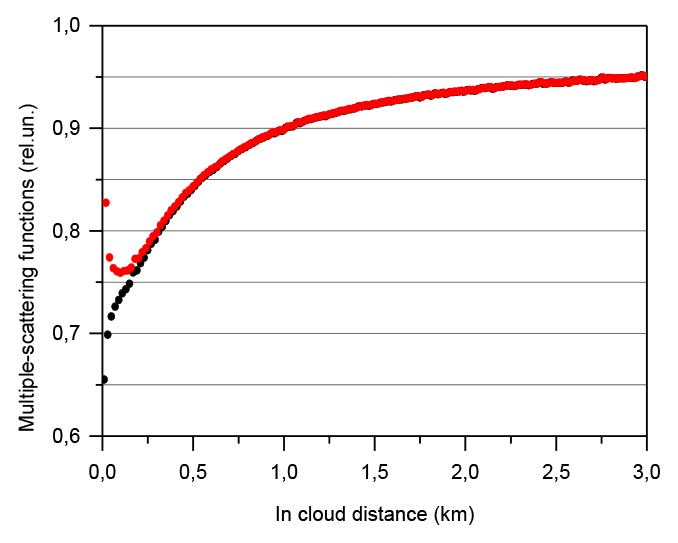
Figure B2 Multiple-scattering function η_MS(h_i): h_i assigned to the middle (black points) and to the end (red points) of the range gate.