the Creative Commons Attribution 4.0 License.
the Creative Commons Attribution 4.0 License.
 | 11 Jan 2022
Optimization of Aeolus' aerosol optical properties by maximum-likelihood estimation
Frithjof Ehlers
Thomas Flament
Alain Dabas
Dimitri Trapon
Adrien Lacour
Holger Baars
Anne Grete Straume-Lindner
The European Space Agency (ESA) Earth Explorer Mission Aeolus was launched in August 2018, carrying the first Doppler wind lidar in space. Its primary payload, the Atmospheric LAser Doppler INstrument (ALADIN), is an ultraviolet (UV) high-spectral-resolution lidar (HSRL) measuring atmospheric backscatter from air molecules and particles in two separate channels. The primary mission product is globally distributed line-of-sight wind profile observations in the troposphere and lower stratosphere. Atmospheric optical properties are provided as a spin-off product. Being an HSRL, Aeolus is able to independently measure the particle extinction coefficients, co-polarized particle backscatter coefficients and the co-polarized lidar ratio (the cross-polarized return signal is not measured). This way, the retrieval is independent of a priori lidar ratio information. The optical properties are retrieved using the standard correct algorithm (SCA), which is an algebraic inversion scheme and therefore sensitive to measurement noise. In this work, we reformulate the SCA into a physically constrained maximum-likelihood estimation (MLE) problem and demonstrate a predominantly positive impact and considerable noise suppression capabilities. These improvements originate from the use of all available information by the MLE in conjunction with the expected physical bounds concerning positivity and the expected range of the lidar ratio. To consolidate and to illustrate the improvements, the new MLE algorithm is evaluated against the SCA on end-to-end simulations of two homogeneous scenes and for real Aeolus data collocated with measurements by a ground-based lidar and the Cloud–Aerosol Lidar and Infrared Pathfinder Satellite Observations (CALIPSO) satellite. The largest improvements were seen in the retrieval precision of the extinction coefficients and lidar ratio ranging up to 1 order of magnitude or more in some cases due to effective noise dampening. In real data cases, the increased precision of MLE with respect to the SCA is demonstrated by increased horizontal homogeneity and better agreement with the ground truth, though proper uncertainty estimation of MLE results is challenged by the constraints, and the accuracy of MLE and SCA retrievals can depend on calibration errors, which have not been considered.
- Article
(8947 KB) - Full-text XML
- BibTeX
- EndNote


Aeolus is an ESA (European Space Agency) Earth Explorer Core mission launched on 22 August 2018 (Stoffelen et al., 2005; ESA, 2008). Aeolus' payload consists of the Atmospheric LAser Doppler INstrument (ALADIN), which is a UV high-spectral-resolution (HSRL) Doppler wind lidar operating at 355 nm wavelength (Chanin et al., 1989; Garnier and Chanin, 1992; Korb et al., 1992; Souprayen et al., 1999b, a; Gentry et al., 2000) and the first Doppler wind lidar in space. The primary mission goal is to provide accurate global measurements of vertical wind profiles in the troposphere and lower stratosphere with global coverage each week for use in operational numerical weather prediction (NWP) and scientific research. Additionally, Aeolus can contribute to the global monitoring of cloud and aerosol optical properties due to the applied aerosol HSRL method (Shipley et al., 1983; Shimizu et al., 1983; Grund and Eloranta, 1991; She et al., 1992; Weitkamp, 2006). Among various space missions that carry active lidar instruments are the Cloud–Aerosol Lidar and Infrared Pathfinder Satellite Observations (CALIPSO), launched in 2006 (Winker et al., 2003); Ice, Cloud and land Elevation Satellites (ICESat and ICESat-2), launched in 2003 and 2018 (Spinhirne et al., 2005; Martino et al., 2019), respectively; and the Cloud–Aerosol Transport System (CATS) deployed on the International Space Station (ISS) in 2015 (McGill et al., 2015). A further mission currently being implemented is the ESA’s Earth Clouds, Aerosols and Radiation Explorer (EarthCARE) scheduled for launch in 2022 (Illingworth et al., 2015). Particularly the combination of CALIPSO, CATS, Aeolus and EarthCARE will potentially offer a detailed and long-term dataset of aerosol and cloud optical properties to the benefit of numerical weather prediction and climate research as the largest single cause of uncertainty in anthropogenic radiative forcing has been reported to be from the indirect effect of aerosols on clouds (IPCC, 2013; Illingworth et al., 2015). This dataset is a unique addition to ground-based lidar networks such as the European Aerosol Research Lidar Network (EARLINET) (Pappalardo et al., 2014) due to the regular global coverage.
The key advantage of ALADIN's HSRL capability is the independent estimation of volume extinction coefficient and co-polarized volume backscatter coefficient products at 355 nm from two different spectral channels. On the other hand, this requires a robust channel crosstalk correction. The Aeolus atmospheric optical property retrieval is implemented in the Level 2A processor, as described by Flamant et al. (2008) and Flamant et al. (2020). Following its launch, the Aeolus atmospheric backscatter signal levels were found to be a factor of 2.5 to 3 lower than expected due to lower laser output energies and a decreased instrument transmission by about 30 % (e.g. Reitebuch et al., 2020). This has caused lower signal-to-noise ratios (SNRs) in the receive channels, and as a result, Aeolus optical property retrieval with the HSRL standard correct algorithm (SCA) is hampered due to high noise sensitivity (see Appendix A). Particularly the particle extinction coefficient retrieval is severely affected due to its dependency on the slope of already-noisy attenuated molecular backscatter signals. In the past, attempts were made to mitigate nonphysical optical properties in the SCA (such as oscillating or negative extinction coefficients in low-aerosol-load conditions) by measures like zero-flooring or signal accumulation in even coarser range bins (Sect. 6.2.2.1 and 6.3 in Flamant et al., 2020) but with limited success. Particle extinction coefficient retrieval from HSRL, and similarly Raman lidar observations, is known to be an ill-posed problem in the presence of any noise (Shcherbakov, 2007; Pornsawad et al., 2008, 2012; Denevi et al., 2017; Garbarino et al., 2016). A classical mitigation approach is to increase the SNR by averaging the data in non-overlapping blocks before processing or application of low-pass filters on either the measured lidar signal or the atmospheric optical properties, i.e. aerosol backscatter and extinction coefficients (Ansmann et al., 2007; Young et al., 2008; Eloranta, 2014; Flamant et al., 2020). Here, the lidar signal is seen as a two-dimensional image with the dimensions range and time owing to continuous operation. But decreased resolution is often not acceptable due to increase in representativeness errors, e.g. when the heterogeneity of the observed atmospheric scene forbids a coarser description in the case of high gradients (broken clouds with aerosols). For Aeolus there is no suitable resolution in between (i) a low-SNR or noise-dominated regime and (ii) a representation-error-dominated regime so that suitable regularization techniques and non-linear regression methods must be applied. The most commonly used methods for retrieval of atmospheric optical properties from active optical remote sensing by lidars are (penalized) least square fit (LSF) (Whiteman, 1999; Pornsawad et al., 2008, 2012), (penalized) maximum-likelihood estimation (PMLE) (Shcherbakov, 2007; Denevi et al., 2017; Garbarino et al., 2016; Marais et al., 2016; Xiao et al., 2020), and the optimal estimation method or Bayesian method (OEM) (Povey et al., 2014; Sica and Haefele, 2015; Donovan et al., 2020). A thorough documentation of the OEM in inverse problems for atmospheric sounding was given by Rodgers (2000), whose notation is adapted in this work for all non-linear regression methods. The strengths of such techniques lie within the characterization and utilization of any additional information, such as the measurement uncertainties or another hypothesis about the state. Such additional information content (if correct) enables a better characterization of the underlying aerosol optical properties. Most of the mentioned works exploit the knowledge of measurement uncertainties and positivity constraints on optical properties and can therefore outperform purely algebraic inversions of particle extinction coefficients. The SCA approach is such a purely algebraic inversion algorithm. Another specific advantage in the works of Shcherbakov (2007), Povey et al. (2014), Marais et al. (2016) and Xiao et al. (2020) is the coupled retrieval of particle backscatter coefficients and extinction coefficients via the particle lidar ratio (extinction-to-backscatter ratio) because particle backscatter coefficients are usually measured with much higher precision. Thus, the particle extinction may occur only where there is backscatter and may vary only in terms of the typical lidar ratio range. This way, the retrieved set of optical properties is automatically consistent in itself and with the underlying physics (assumptions).
In this work, we want to explore and demonstrate the potential of non-linear regression in Aeolus' aerosol optical property retrieval. The already-implemented SCA approaches serve as a benchmark for comparison. Therefore, the retrieval problem is reformulated into a maximum-likelihood estimation (MLE) problem, which aims to solve the noted issues in the SCAs as follows: firstly, we account for the noise of the signals in both channels; secondly, we suggest that particle backscatter and extinction coefficients are retrieved in a coupled way; and, thirdly, we constrain the solution space to a physically reasonable subset only. This means constraining the lidar ratio to values in between 2 and 200 sr and setting a positivity constraint on extinction and backscatter coefficients. A considerable gain in the quality of the retrievals is expected, particularly due to the latter two measures, because a coupled retrieval in conjunction with a box-constrained set of space variables will allow for important information exchange during the determination of the self-consistent set of optical properties. Therefore, our method differs from the approaches in Shcherbakov (2007), Marais et al. (2016) and Xiao et al. (2020), which first obtain backscatter coefficients and successively calculate extinction coefficients. It is important to note that such a simultaneous retrieval with ground-based lidars would require the additional geometric overlap function calibration parameter. Hence, it is often preferred to retrieve backscatter coefficients independent of extinction coefficients to mitigate biases in the former due to calibration errors. The developed MLE framework naturally offers the potential to be further refined into an optimal estimation method (OEM) or penalized maximum-likelihood estimation (PMLE) method due to the strong similarity between the methods.
This paper is structured as follows: a brief instrument description in Sect. 2 is followed by a recap of the classical retrieval algorithms (SCAs) and their underlying set of equations and the MLE approach in Sect. 3. In Sect. 4, results are presented and discussed from the comparisons of the SCA and MLE approaches using end-to-end simulations of homogeneous standard atmosphere scenes, real Aeolus observations of a Saharan Air Layer event and Aeolus observations collocated with ground-based lidar observations near Tel Aviv. The final section provides the study conclusions and outlook.
Aeolus revolves around the Earth in a sun-synchronous polar orbit at about 320 km altitude with a 7 d repeat cycle. The ALADIN instrument emits a narrow-bandwidth UV laser pulse close to 355 nm wavelength, and the instrument is pointing to Earth with an off-nadir slant angle of 35∘ measured from the spacecraft, which accounts for an approximately off-nadir angle at the Earth's surface due to Earth's curvature. The diameter of the laser footprint is about 12–15 m, and the instrument field of view is 19 µrad. The laser light is backscattered by particles (aerosol and hydrometeors resulting in spectrally narrow Mie scattering) and air molecules (resulting in thermally and pressure-broadened Rayleigh–Brillouin scattering). The frequency of the atmospheric backscattered laser light is Doppler-shifted relative to the emitted frequency owing to the relative velocity of the scattering media (wind speed) along the instrument line of sight (LOS). The contributions of Earth's rotation and satellite movement are compensated by Aeolus' attitude control and on-ground data processing such that the Doppler shift is entirely dominated by the LOS wind speeds. In order to measure the LOS wind speeds, Aeolus utilizes two different receiver spectrometers, namely a fringe imaging Fizeau interferometer for the spectrally narrow Mie backscattered laser light and two sequential, double-edge Fabry–Pérot interferometers for the spectrally broad Rayleigh backscatter. Hence, continuous LOS wind speed profiles up to 30 km altitude can be measured regardless of the presence and absence of aerosol, unless optically thick features such as dense liquid water clouds block the beam. Additionally, the measured signal intensities allow a retrieval of particle optical properties.
The core of ALADIN is its diode-pumped frequency-tripled Nd:YAG laser with 80 mJ nominal pulse emit energy and 50 Hz pulse repetition frequency. The emit beam is circularly polarized, but the cross-polarized part of the backscattered light is discarded in the receive path optics due to the instrument design. Hence, in the case of strongly depolarizing targets, the signal measured at the detectors is strongly reduced with respect to non-depolarizing targets (ESA, 2008; Flamant et al., 2020). Additionally, the expected atmospheric return signal in orbit is a factor of 2.5 to 3 lower than expected before launch due to lower laser output energies than originally intended (45–72 mJ) and decreased instrument transmission by about 30 %, which has caused a lower SNR since mission start (Reitebuch et al., 2020).
The light backscattered from the atmosphere is an attenuation of Mie and Rayleigh backscatter, which is then separated by the two instrument receivers. Figure 2 in Ansmann et al. (2007) illustrates how the spectral characteristics of the Mie and Rayleigh backscatter are exploited to separate them with the spectrometers (channels) (Ansmann et al., 2007; Reitebuch et al., 2018a). If the LOS wind speed is non-zero, the whole spectrum will be shifted relative to the channel transmission curves due to the Doppler shift. The light first travels to the Mie receiver, where the narrow Mie peak (fringe) is measured to determine this Doppler shift directly. The frequency-broadened Rayleigh scattered light gets reflected on the Mie channel and is then directed to the two Rayleigh channel filters. These capture different signal intensities in the two filters centred on each side of the centre emit frequency. By comparing and normalizing the responses in the two filters, the LOS wind Doppler shifts can be calculated. However, the return signals from particles (Mie) and molecules (Rayleigh) are not entirely separated due to the overlap of the transmission functions of the two channels and the sequential design of the receivers. Therefore, channel crosstalk is present, which needs to be corrected to obtain unbiased LOS wind and optical properties.
The atmospheric echoes from the single pulses passing through the instrument receivers are collected with time-gated accumulation charge-coupled devices (ACCDs). The time it takes for the light to travel from the instrument, through the atmosphere and back to the receivers is used to accumulate the light from the individual pulses over time equivalent to atmospheric vertical bins of 250 m. The same ACCDs, with a quantum efficiency of 85 %, are used for both the particle (Mie) and molecular (Rayleigh) channels. In order to achieve sufficient charge build-up before read-out and digitalization, 19 laser pulses are accumulated directly on the storage columns of the ACCD. The accumulation of 19 laser pulses corresponds to an on-ground distance of about 2.9 km along track and is the smallest horizontal measurement which is down-linked to Earth. Individual, vertical range bin sizes can be independently varied between 250 and 2000 m in steps of 250 m while remaining limited to a total number of ACCD rows and hence vertical range bins of 25 per column. Of these range bins, one is used for solar background measurements, and one is used to sample the ground. In order to achieve the mission requirements for random wind errors, a number of measurements are added up at a coarser scale during the on-ground processing. For Rayleigh winds, a total of 30 measurements are accumulated to one basic repeat cycle (BRC) or observation (Aeolus mission terminology), equivalent to approximately 87 km along-track distance on the ground. Mie winds can be provided at smaller scales dependent on the SNR of the aerosol feature. High SNR is also critical for optical property retrieval, particularly particle extinction coefficients. Hence, optical properties are primarily evaluated at the observation scale as well and only refined afterwards in what is called the group product. An example of raw signals at the measurement scale (2.9 km) accumulated at the observation scale (87 km) is given in Fig. 1, which shows the test case discussed in Sect. 4.3.
The geolocated measurement data from the satellite, including detected Doppler shifts and the useful signals from the two Rayleigh channels and the Mie channel, are provided in the Level 1B (L1B) data product (Reitebuch et al., 2018a). These are the signals that have been corrected for the detection chain offset (DCO; measured for all range bins in separate, non-illuminated pixels), dark current charge offset in memory zone (DC or DCMZ; from on-ground characterization), tripod obscuration (TOBS; in Mie channel only) and the solar background contribution (measured in range bin 25 for all channels) (Reitebuch et al., 2018a). The L1B product in combination with additional calibration data from the CAL Suite processing step and meteorological information from a global weather forecast from the European Centre of Medium-Range Weather Forecasts (ECMWF) is used as input by the optical property processor to generate the Level 2A (L2A) data product (Flamant et al., 2020). The calibration data are obtained from designated instrument modes and internal reference measurements (Reitebuch et al., 2018a). Within the L2A product, three different algorithms are implemented: the first is the standard correct algorithm (SCA), which makes use of the full HSRL potential and uses both channels to retrieve lidar ratios directly from the data. The second is the Mie channel algorithm (MCA), which applies a Klett-like retrieval (Klett, 1981; Fernald, 1984) with an a priori lidar ratio value (extinction-to-backscatter ratio). The third, the iterative correct algorithm (ICA), intends to refine the SCA results at finer vertical scales but fails to generate reasonable results in the nominal operation due to pronounced sensitivity to noise. Hence, given its more accurate approach and better performance, only the SCA is considered in the remainder of this paper.

The atmospheric forward model in lidar applications is based on the lidar equation (Weitkamp, 2006). In its simplest form, the lidar equation reads
The signal power s received from distance r is made up of four factors. The constant K summarizes the signal transmission through the lidar instrument, and contains all range-dependent terms regarding the measurement geometry. For Aeolus the range overlap function O(r) equals 1. The two unknown terms that contain information on the atmospheric state are the total backscatter coefficient β(r)>0 at distance r and the atmospheric transmission that describes how much light gets lost on the way from the lidar to the target at a distance r. In the following, we consider the case of the single-scattering approximation; i.e. multiple-scattering effects are neglected. As discussed in Flamant et al. (2008) and Ansmann et al. (2007), this is a valid assumption due to the small divergence and narrow field of view (FOV) of the ALADIN instrument. In the case of ALADIN, the lidar equations for the two channels read
with the Mie and Rayleigh channel signals s, laser pulse energy E0, number of accumulated pulses Np, atmospheric temperature t, atmospheric pressure p, Doppler shift f, instrumental calibration constants Kray and Kmie, and crosstalk coefficients C1…4 accounting for the fractions of molecular and particulate signal in the Rayleigh and Mie channel, respectively. The total backscatter coefficient has been split into a molecular contribution and particle contribution . Here, βp is explicitly split into the cross-polarized and co-polarized fraction , of which only the co-polarized particle backscatter coefficient is measured due to instrument design. denotes the two way transmission
with range-dependent extinction coefficient α and label m for molecules and p for particles, respectively. The two unknown parameters of interest are co-polarized particle backscatter coefficient and particle extinction coefficient αp, which can, in principle, be solved with the two equations because and hold true by instrument design. In the following, we also make use of the co-polarized lidar ratio (extinction-to-backscatter ratio) . Since the co-polarized particulate backscatter is lower than the total particulate backscatter βp, the co-polarized lidar ratio overestimates the true lidar ratio (). The lidar equations can be simplified by introduction of the range-resolved atmospheric signals at telescope entry
with X(r) for molecular backscatter and Y(r) for particulate backscatter in units of m−3 sr−1. These resemble normalized signals that would be obtained in the absence of channel crosstalk. So the lidar equations read
where variable dependences are dropped for the sake of readability.
The instrument is calibrated with measurements from dedicated instrument calibration modes (Reitebuch et al., 2018a), and the crosstalk coefficients C1…4 are determined according to Flamant et al. (2020) and the procedure in Dabas (2017). At (1000 hPa, 300 K, 0 MHz), C1 and C4 equal 1 by definition. The other coefficients then typically take values of about C2≈0.5 and C3≈1.25. For the rest of this work, we assume the calibration as known and do not include the contribution of calibration errors in the results. The calibration cannot be perfect in reality but is likewise input to all algorithms, which guarantees a fair comparison of retrieval precision in Sect. 4.3 and 4.4.
3.1 Standard correct algorithm (SCA)
For a more detailed description of the SCA and a discussion of its shortcomings, we refer to Appendix A and Flamant et al. (2020). In the following, the index as subscript to the properties above denotes the range bin index. This implies for the signals s, X and Y that the property has been integrated over a discrete range , i.e. . For all other variables like backscatter coefficients β, extinction coefficients α and range R, this subscript denotes the average in range bin i, i.e. , with and equivalently for subscript m. As a consequence, particle optical depth of a bin is denoted . The following approximations for the range-corrected signals (Eqs. 5 and 6) are made by using the mean bin properties from above (see Eqs. 6.35–6.36 and definitions above in Flamant et al., 2020):
with unknown optical depth Lp,sat in between the telescope and first range bin. With Eqs. (7) to (10), the SCA solves algebraically for the two unknowns, co-polarized lidar ratios and optical depths Lp,i (and Lp,sat), which are equivalent to extinction coefficients αp,i and backscatter coefficients (and Lp,sat). Backscatter coefficients are simply retrieved from . The SCA produces two sets of products, the SCA and the SCA midbin (SCA MB) backscatter and extinction coefficient profile products and lidar ratios. The SCA attempts to regularize the solution by not allowing negative optical depth within the iterative retrieval (zero-flooring). The SCA midbin product does not implement such a constraint but averages the SCA neighbouring bins at a coarser resolution in order to dampen oscillations in the retrieved profiles in scenes with low signals in order to obtain a more stable product. Further details of the products and their performances are provided in Sect. 4 and Appendix A.
3.2 Maximum-likelihood estimation (MLE) retrieval
The basis of MLE and OEM methods is formed by the forward model y=F(x), which maps physical properties from state space onto measurement space (Rodgers, 2000). We use Eqs. (7) to (10) in order to calculate the measurement space variables (signals) from the state space variables (optical properties) with
The deviation between the actual measurement and the forward-modelled state is represented by a cost function that needs to be minimized to obtain a good estimate of the underlying true state. Generally, the cost function in non-linear regression problems is composed of two terms
of which the first describes deviation from the measurement and the second the deviation from some a priori state (applied in the OEM) or from another a priori constraint (applied in PMLE), e.g. smoothness. The second term is also referred to as the penalty term. In MLE, J is the log-likelihood function, which in the case of normally distributed measurement errors becomes the weighted least squares term
with measurement error covariance matrix Sy (compare to Eqs. 2.21 or 5.3 in Rodgers, 2000). Often the choice of Poisson noise in conjunction with the Kullback–Leibler divergence is preferred in lidar applications (Denevi et al., 2017; Marais et al., 2016; Garbarino et al., 2016; Weitkamp, 2006) because photon shot noise is the dominant noise source for the signals on the detectors, which is fairly Poisson distributed. Here, we do not restrict noise amplitudes to the Poisson case to account for additional noise contributions, such as laser pulse frequency jitter, ACCD readout noise, dark electron and thermal noise contribution, and potentially unknown “noise” sources such as atmospheric variability. The description of Jobs in terms of normal distributions is not a critical aspect of the method because the discrete Poisson noise distribution can be decently well approximated by a smooth Gaussian distribution with identical mean and variance for very low (photon) counts, and the aforementioned additional noise sources and their corrections, e.g. subtraction of measured solar background, will naturally smear out the discrete nature of the Poisson noise. For the time being, no explicit a priori term contributes to the cost function used throughout this work, although limits will be imposed on the state space variables by specifically solving the box-constrained MLE problem
with box constraints on lidar ratio, which is prior information that cannot be exactly represented by the OEM. The state that solves this minimization problem (Eq. 14) is denoted x*. It is important to mention that it is only the a priori knowledge in the form of the box constraints that makes the MLE solution distinct from the algebraic SCA solution (without zero-flooring; see Sect. 6.2.2.1 in Flamant et al., 2020) because this algebraic solution corresponds to the exact signal values in y and therefore to Jobs=0, which is the global minimum of the unconstrained counterpart of the problem (Eq. 14). Due to the implemented zero-flooring of optical depth in the SCA, its retrieved optical properties do not correspond perfectly to the measured signals (see also Fig. 7 in Flament et al., 2021), though Jobs=0 still holds in the case of the unregularized SCA MB retrieval. In practice, the minimization problem (Eq. 14) needs to be solved for all optical property profiles along the Aeolus orbit. So instead of solving Eq. (14) per single atmospheric column, it is solved for all columns at once (at the observation scale). Without loss of generality, this can be realized by minimization of the sum of the single cost functions
over all N lidar profiles with index k. This is equivalent to the ensemble of the separate minimization problems because the kth cost function is strictly positive and only sensitive to changes in the kth state vector. So the collection of state vectors that minimize the sum of the cost functions have to minimize each summand independently. This way, we gain the freedom to use the inherent 2D information of the lidar signal in future developments, e.g. to couple neighbouring profiles by the introduction of a regularization term to Eq. (15) that acts on the horizontal direction along the satellite orbit (Marais et al., 2016; Xiao et al., 2020).
In theory, extinction and backscatter coefficients can be chosen as a state space description as well as lidar ratio and backscatter . However, the reason to favour a state space description containing the lidar ratio is that such states can be easily constrained to physical bounds by forcing upper and lower ranges within the retrieval. Within the description, the lidar ratio constraint would become non-linear and harder to handle by off-the-shelf tools for numerical optimization. The crosstalk-corrected signals Xi and Yi instead of the Rayleigh and Mie channel signals sray,i and smie,i are an equally valid choice of the measurement space variables y, but then the measurement covariance matrix Sy would have off-diagonal entries due to the linear transform in Eqs. (A4)–(A5). The above choice has been made for the sake of simplicity and to simplify the cost function and its gradients since the signals in separated vertical range bins are expected to be uncorrelated except for a small range bin overlap (Weiler, 2015). This overlap is about ±120 m altitude for Mie ACCD and ±30 m for Rayleigh ACCD in nominal operation and regardless of range bin settings. As in the SCA, this overlap is not considered in this work.
As pointed out by Povey et al. (2014), unbiased uncertainty estimates are a prerequisite to obtain good results. This is an issue for low signal intensities when estimating the Poisson uncertainty from the uncertain signal s itself: the uncertainty will be biased by the exact noise value in the signal because a single draw in general does not equal the true mean and the true variance. In Aeolus L1B data products, the Poisson noise assumption is applied to calculate signal-to-noise ratio (SNR) in both signal channels, including the solar background contribution. For Eq. (14), we use instead the variance measured at 2.9 km resolution, scaled to approximate the noise level in the 87 km bins. This approximation assumes the scene is homogeneous so that all the variability is due to measurement error (see Appendix B). Note that the position of a cost function minimum is invariant to scaling of the covariance matrix Sy→λSy with scalar λ, while the relative magnitude of its entries is important when being subject to constraints, i.e. in a general case where J>0 holds at the minimum.
The choice of the upper and lower lidar ratio bounds takes the following points into consideration: on one hand, the true lidar ratio at 355 nm is expected to exceed values of 100 sr only in rare cases, and a physically lower bound might be presented by approximately 10 sr (see Fig. 8 in Illingworth et al., 2015, or Wandinger et al., 2015). On the other hand, the coarse vertical resolution and the effects of depolarization need to be accounted for. Therefore, highly depolarizing aerosol, such as desert dust and ice particles in cirrus clouds, will appear to be highly attenuating since the co-polarized lidar ratio can be increased by a factor of up to 1.85 for desert dust and 3 for cirrus clouds compared to the true lidar ratio. Taking into account typical distributions of lidar ratios and depolarization values as in Wandinger et al. (2015); Illingworth et al. (2015), values as high as 130 sr will be well within physical limits for Aeolus. On the other hand, as shown in Flamant et al. (2020), aerosol partially filling a range bin can cause the retrieval results to underestimate the true particle extinction by a factor of 16 and therefore underestimate the lidar ratio. The applied bounds need to account for these forward model errors by an extra margin. All things considered, the limits of 2 to 200 sr resemble a reasonable trade-off.
The minimization problem (Eq. 15) is solved approximately by a Limited-Memory Broyden–Fletcher–Goldfarb–Shanno algorithm with box constraints (L-BFGS-B), a quasi-Newton code for bound-constrained optimization. More precisely, the implementation described in Zhu et al. (1997), version 3.0, is used. As an addition, the cost function gradient is evaluated efficiently via automatic differentiation. The initial conditions, or the first guess, consist of an aerosol-free atmosphere with Lp=0 and a lidar ratio of sr. Since the L-BFGS-B algorithm is not invariant under variable transforms, it was necessary to introduce an additional scale parameter in the state vector for good convergence rates of the cost function. The applied transformation maps Lp→200Lp in the state vector to ensure that all entries are about the same order of magnitude. More advanced variable transforms such as pre-whitening of the variables (Rodgers, 2000) may be appropriate to optimize performance, but the proposed rescaling is found to be sufficient.
MLE estimates may suffer from overfitting and noise amplification in lidar retrieval problems, so an implicit regularization is often achieved by optimal choice of the number of iterations (Denevi et al., 2017; Garbarino et al., 2016). But we suppress noise amplification by the box constraints. So, the L-BFGS-B iteration is stopped after a predefined number of iterations of 40 000, after which the average cost function value per bin is required to be smaller than 1. Usually, this holds true after far fewer iterations (∼50 for the single column problem (Eq. 14) and ∼5000 for the problem (Eq. 15) with about 450 profiles), but in the spirit of the SCA, the estimate should fit as close as possible to the signal data and only solve the physical contradictions. Hence, a fair comparison to the standard algorithms is achieved only without an implicit regularization. For operational use we plan to tune the number of iterations in an ad hoc fashion based on when the average cost function value per bin has fallen below a value of 1.
A Monte Carlo approach as in Xiao et al. (2020) is applied to classify the uncertainties in simulation results in Sect. 4.1 and 4.2. For this, a sufficient number of realizations of the measurement vector yobs are generated from the homogeneous simulation scene. The variation in the SCA- and MLE-estimated state vector x* then yields a reliable measure of the retrieval variability and the standard error. Such a Monte Carlo approach is the most representative of the algorithm performance but cannot be applied to real observation data, where the noise is unknown and cannot be varied.
The uncertainties in SCA and SCA MB retrievals in observational data are operationally calculated via standard error propagation (see Eqs. 6.54–6.100 in Flamant et al., 2020) and under the assumption of pure Poisson noise in signals s. While a similar analysis can be made for the MLE, we find that especially the obtained extinction uncertainties would strongly overestimate the actual variability in MLE results due to the omitted constraints in such a procedure. Hence, future work regarding the implementation of the box constraints in the error estimation is pending.
In this section, the two versions of the SCA and the MLE algorithms are tested on synthetic and real Aeolus observation test cases, and their performances are discussed. The simulated data are produced with the Aeolus end-to-end simulator described in Reitebuch et al. (2018b), which allows realistic simulations of ALADIN measurements from defined atmospheric scenes as input to the L1B algorithm. Its output data are provided in the same format and temporal and spatial resolution as nominally downlinked from the satellite in order to test the whole processing chain up to the optical properties delivered in the L2A product. The simulation covers the charge transfer and detection on the accumulation charge-coupled device (ACCD) including offsets, non-linearity and noise sources, such as dark current noise, read-out noise, Poisson detection noise (shot noise) and the analogue-to-digital conversion with 16 bit. Although perfect agreement with the instrument on board cannot be achieved, the simulated noise level resembles nominal operations. Four simulated and real Aeolus observation test cases have been defined as follows:
-
atmospheric simulation case I – a horizontally homogeneous aerosol profile
-
atmospheric simulation case II – case I with an additional cloud
-
real data case I – a Saharan Air Layer (dust plume) above Cape Verde
-
real data case II – a ground-based comparison with a Polly XT lidar in Tel Aviv.
In the following sections, the results from each test case are presented.
4.1 Atmospheric simulation case I
The simulated Aeolus observations from this test case are obtained from the end-to-end simulator and contain horizontally homogeneous aerosol with a constant lidar ratio of 25 sr, and the calibration data are known from separate simulations of Aeolus' calibration modes. A standard atmosphere temperature and pressure distribution are used for the simulation of the molecular backscatter with altitude, and the wind speed is zero for simplicity. The simulated atmospheric scene contains aerosol up to 40 km altitude, particularly above Aeolus' range of about 0–20 km. This aerosol attenuates the useful signals by an additional 0.9 %, but no impact is expected on the optical properties since all algorithms allow for a constant attenuation factor.
The retrieval results for the simulation are shown for the SCA, SCA midbin and MLE algorithms in Fig. 2. Please note the logarithmic scales of the colour bar. The medium aerosol load in the input atmosphere with backscatter coefficients on the order of 1 to 10 Mm−1 sr−1 below 2 km is captured well by all algorithms (rows 1 and 2 of Fig. 2). However, clear background noise patterns are visible in the optically thin aerosol regime with particle backscatter coefficients on the order of order 0.1 Mm−1 sr−1 above 2.5 km for all retrievals, as expected due to low Mie channel SNR (rows 1 and 2 of Fig. 2). Hence, there are many noise-induced negative values in SCA and SCA midbin retrievals. Additionally, SCA and SCA midbin backscatter profiles are shown to be biased in this regime. The MLE mean profile resembles the true backscatter profile, mitigates negative values, and consistently shows smaller standard deviation than the SCA and SCA midbin. In order to better illustrate this, the bias and relative error for all retrievals with respect to the true profile are presented in Fig. 3. Here, the maximum backscatter coefficient bias in the aerosol layer below 2 km is reduced from about 43 % with the SCA and SCA MB to 27 % with MLE. The bias is collocated with the change in range bin size. We argue that its origin is the non-linear way the backscatter coefficient is calculated from because here will become biased high increasingly with increasing uncertainty in Xi. Because values of Xi are constrained to a physical subset in MLE, they are less variable, and less bias is observed. The relative error in backscatter coefficients is consistently lower for MLE compared to the SCA; in the most interesting area below 2 km the relative error in backscatter coefficients reduces to 50 %–30 % with MLE compared to 120 %–50 % for the SCA, while MLE performs only slightly better than the SCA MB.
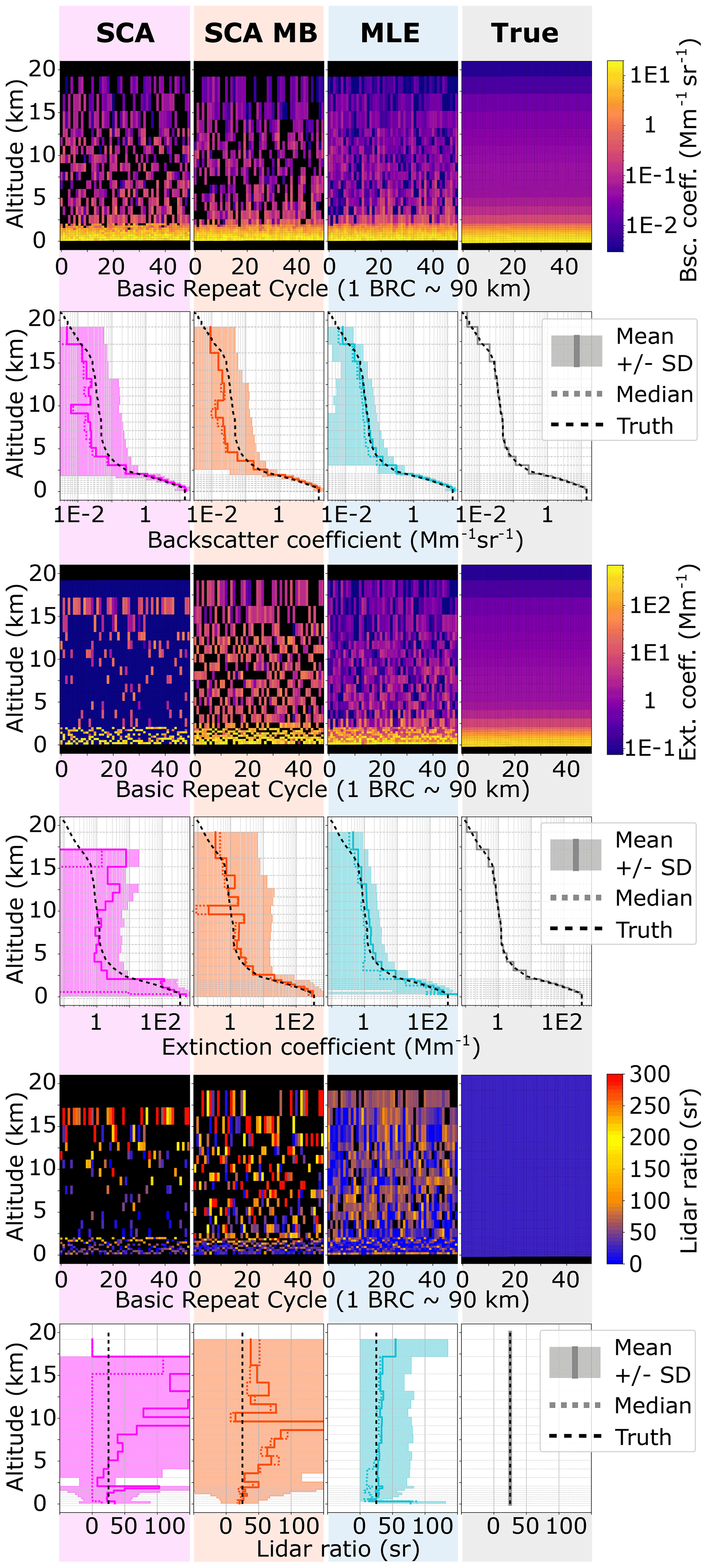
Figure 2Simulation case I: optical property retrieval results. Applied algorithms (from left to right) are the SCA, SCA midbin, MLE and the true simulation input (rightmost). Curtain plots (rows 1, 3 and 5): dark-blue values may exceed the lower colour bar limit, and black colour indicates negative (or missing) data. Statistics (rows 2, 4 and 6): mean profiles (solid lines), ± standard deviation (shaded) and median (dotted) obtained from 1000 BRCs.
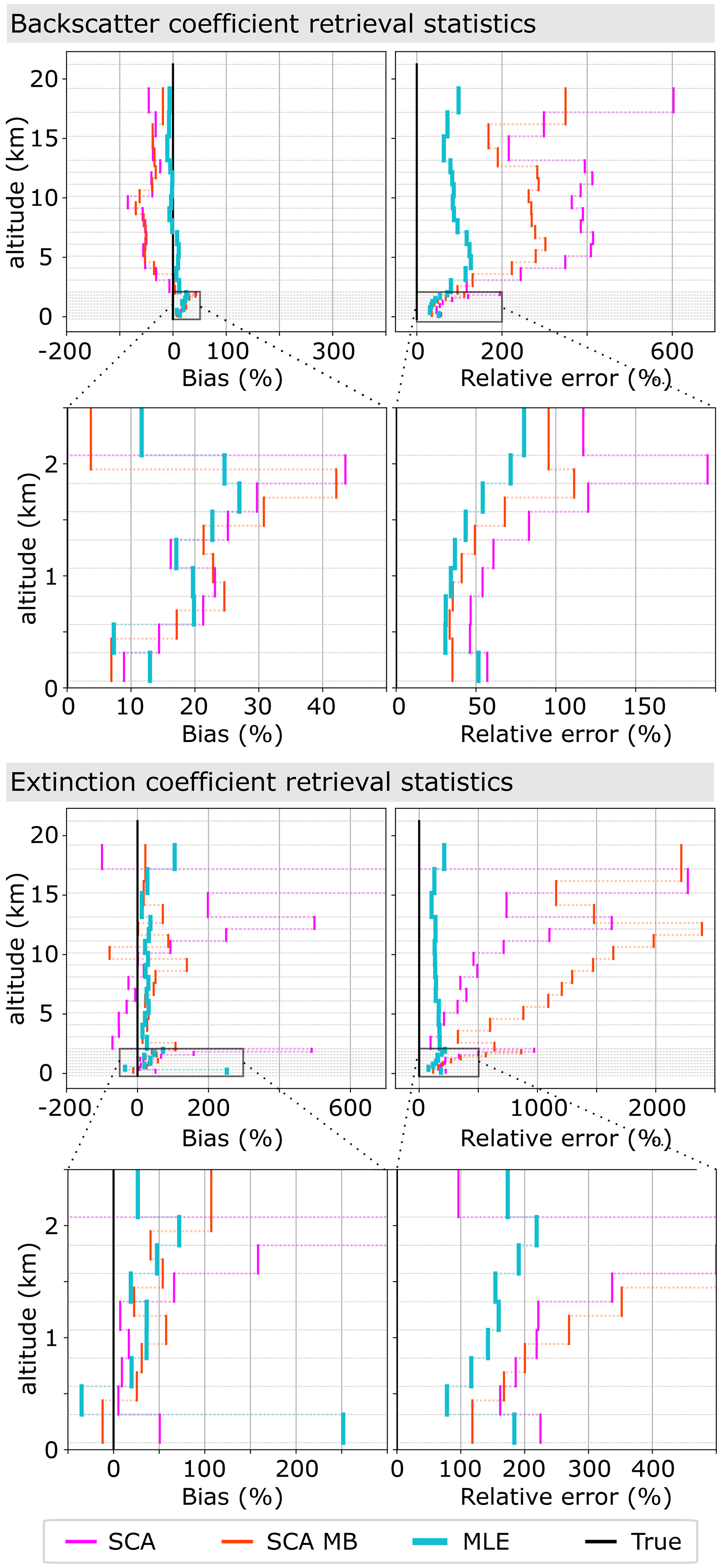
Figure 3Simulation case I: retrieval statistics for backscatter and extinction coefficients obtained from the mean profiles from Fig. 2. Left: bias relative to simulation input parameters. Right: standard error relative to simulation input parameters. Please note the varying x-axis scales.
The coupled retrieval in the MLE unfolds its whole potential in the extinction retrieval (rows 3 and 4 of Fig. 2): the curtain plots for the SCA and SCA midbin suffer not only from intense background noise, but also from negative values within the dense aerosol close to the ground, whereas the MLE achieves a much more robust retrieval when compared to the simulation input. The mean profiles unveil high biases in the SCA case (see also Fig. 3): especially changes in vertical range bin thickness impose a challenge and are followed by extinction overestimation (see biases at 2 and 13 km altitude in Fig. 3) due to the feedback between zero-flooring of extinction coefficients within the processing and decreased SNR in thin bins (see Appendix A). A detailed explanation of the noise influence on the SCA extinction retrieval can be found in Flament et al. (2021). The SCA midbin is less biased, despite a spurious oscillation at about 10 km altitude, but at the price of high noise and lowered resolution. With the exception of the bin closest to the surface, the MLE retrieves the least biased extinction coefficients over the whole profile with standard errors up to a magnitude smaller than the SCA midbin product (see Fig. 3). Retrieved extinction coefficients are all biased high in the area below 2 km, with a maximum bias of 500 % for the SCA, 110 % for the SCA MB and 70 % for MLE. Between 1.5 and 0.5 km altitude, the biases are comparable in magnitude, at about 30 %. Concerning the relative extinction errors, an improvement by a factor of about 1.5 to 2 in comparison to the SCA and SCA MB is achieved by MLE in the lowermost 2 km. However, the relative error is on the order of 100 % or greater in all cases. Only the extinction in the bin closest to the ground appears overestimated with MLE. Deviation from the ground truth was expected due to the diminishing influence of the lowermost optical depth on the cost function.
The lidar ratios in row 6 (lowest panel of Fig. 2) are calculated from and of rows 2 and 4 and their respective standard deviation in order to disregard the influence of bins with nearly vanishing aerosol optical depth, for which the lidar ratio is arbitrary and which have diverging error. The lidar ratio results (rows 5 and 6 of Fig. 2) indicate that the MLE is the most robust as it is the only algorithm for which the lidar ratio statistics converge to the true value of 25 sr nearly everywhere. The SCA and SCA midbin achieve this only in a narrow range close to the ground. The SCA and SCA midbin produce either very high (yellow to red values) or zero or negative (black) values in these cases.
4.2 Atmospheric simulation case II
In simulation case II, the aerosol profile is the same as for case I, but in addition a cloud is placed between 8.5 and 10.5 km with an optical depth of 0.4, i.e. the return signals from below the cloud are more than halved by a slant two-way transmission of (see Fig. 4). The discontinuity of the cloud (abrupt changes in optical properties) introduces some artefacts into the retrieval results, as can be seen in Fig. 4: most prominently, the vertical extent of the cloud is overestimated by the SCA midbin due to the averaging of neighbouring bins at a coarser resolution (rows 1 to 4). Hence, the cloud thickness appears to be 4 km compared to 3 km in the SCA and MLE and 2 km in simulation input parameters. Furthermore, the SCA extinction coefficient reacts delayed compared to the SCA backscatter coefficient, leading to the attenuation by the first 500 m of the cloud not being correctly captured (compare to ground truth in row 3 of Fig. 4), with consequences for lidar ratio estimation. The SCA extinction coefficient values below the clouds are biased high due to the abrupt change in signal error. Hence, the same feedback loop is triggered as described in simulation case I for changes in range bin thickness.
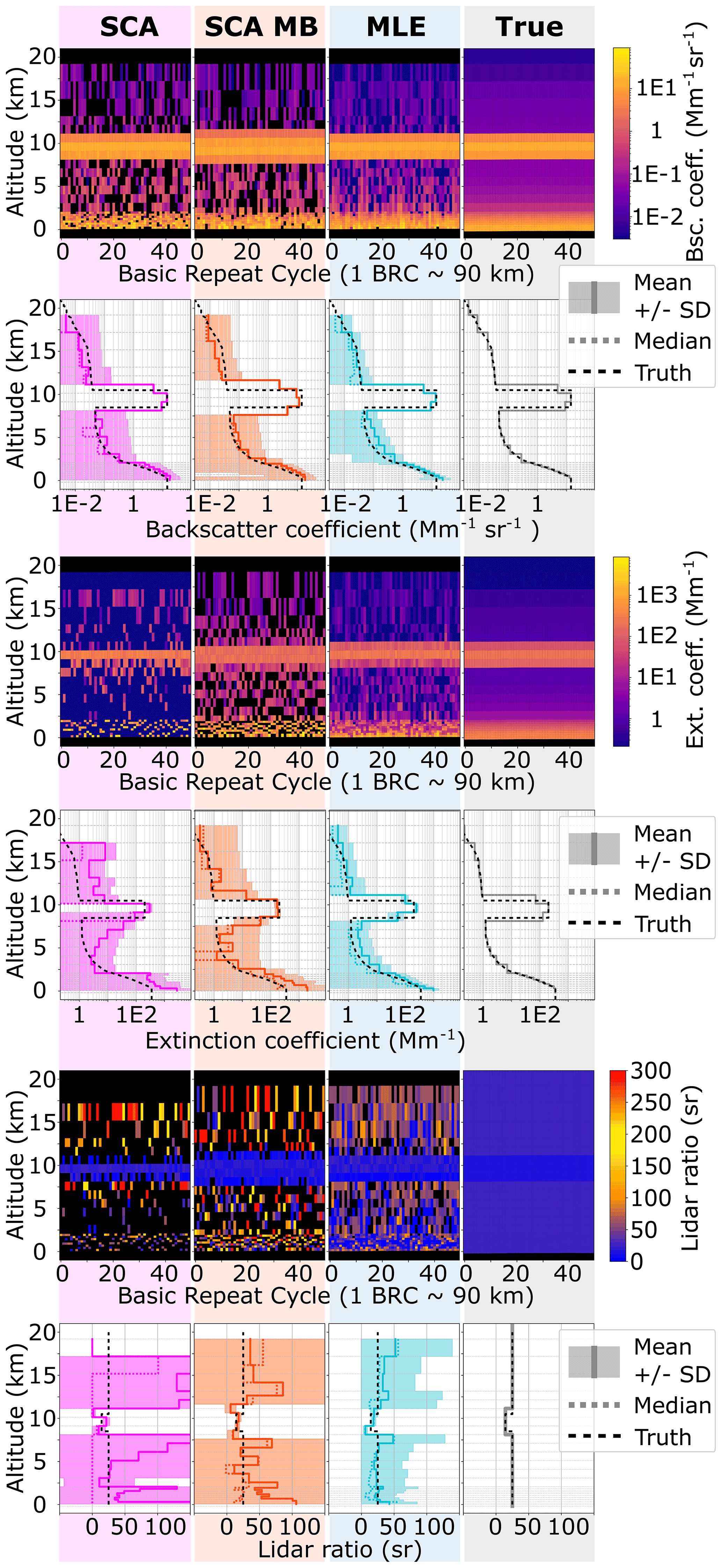
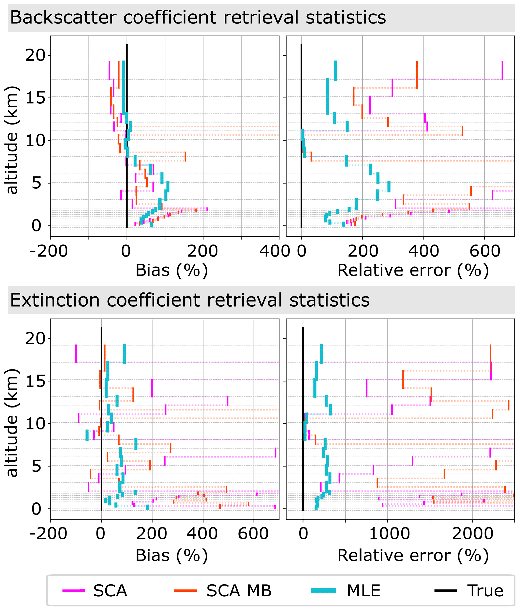
The curtain plots of the SCA and SCA midbin optical properties (rows 1, 3 and 5) reveal more noise-induced negative values (black) below the cloud. MLE provides the backscatter estimates with the highest precision and is the only algorithm for which the relative error drops below the 100 % mark (see Fig. 5). The high backscatter coefficient bias in the lowermost 2 km is more pronounced in all algorithms as compared to atmospheric simulation case I, supporting the hypothesis that it originates from the non-linear ratio operation rather than the gradient of the aerosol concentration. Consequently, due to its noise suppression capabilities, that is likely why MLE shows less bias in the lowermost 2 km. A similar statement can be made for the extinction because it is essentially calculated from a ratio of subsequent pure molecular signal values Xi. A distinct feature of the MLE result is the bias of up to 100 % between 2 and 8 km altitude, which might be introduced by the positivity constraint in conjunction with high noise. However, the bias in the area of interest below 2 km is found to be the lowest in the MLE case. In general, the statistics below the cloud are heavily impacted by the signal loss: extinction coefficient estimates below 2 km are found to be biased extremely high in SCA and SCA midbin results, and so MLE returns the best fit to the simulation input parameters (row 4 in Fig. 4). Nevertheless, Fig. 5 reveals that the bias in MLE extinction coefficients below 2 km is only acceptably small at about 1 km altitude, namely about 20 %. Rows 5 and 6 in Fig. 4 indicate that regardless of the aforementioned biases, the MLE average lidar ratio remains quite accurate compared to the SCA and SCA MB and is furthermore the estimate with the highest precision. This suggests that the noise-induced biases in extinction and backscatter are almost balanced, which can be motivated by the fact that both variables depend on in the forward model (the aerosol optical depth equals the normalized log derivative of pure molecular signal and can be rewritten in terms of the ratio ). Hence, the potential of MLE to cope with highly noisy data compared to the standard approaches is well demonstrated. The SCA and SCA midbin produce either very high (yellow to red values) or zero or negative (black) values in these cases.
In summary, the coupled MLE forces extinction and backscatter to appear collocated and thus consistently outperforms the standard approaches in terms of both accuracy and precision.
4.3 Real data case I: classifying a Saharan Air Layer with Aeolus
In this section, the algorithms are tested and compared using real Aeolus observations from 30 June 2020 during the Aeolus satellite overpass close to Cape Verde between 07:30 and 07:40 UTC. The satellite passed above an extended Saharan Air Layer (SAL; Prospero and Carlson, 1980) containing significant amounts of desert dust. The spatial extent of this dust layer is visible in observations of the UV aerosol index reported by the Copernicus Sentinel-5p TROPOMI instrument (ESA, 2018) between 12:00 and 15:30 UTC. Later that day, NASA's Cloud–Aerosol Lidar and Infrared Pathfinder Satellite Observations (CALIPSO) (Winker et al., 2003) made another overpass over Cape Verde between 15:20 and 15:30 UTC, which crossed Aeolus' ground track, passing over the SAL (see Fig. 6a). CALIPSO carries the polarization-sensitive dual-wavelength attenuated backscatter lidar, CALIOP. The fairly uniform and large SAL layer is an ideal case to compare the CALIPSO vertical feature mask (VFM) product (v4.20, data release version 4.10) and the different Aeolus optical property products. The publicly available L1B data product of baseline 1B10 is used as input to the L2A optical property prototype processor version 3.12.
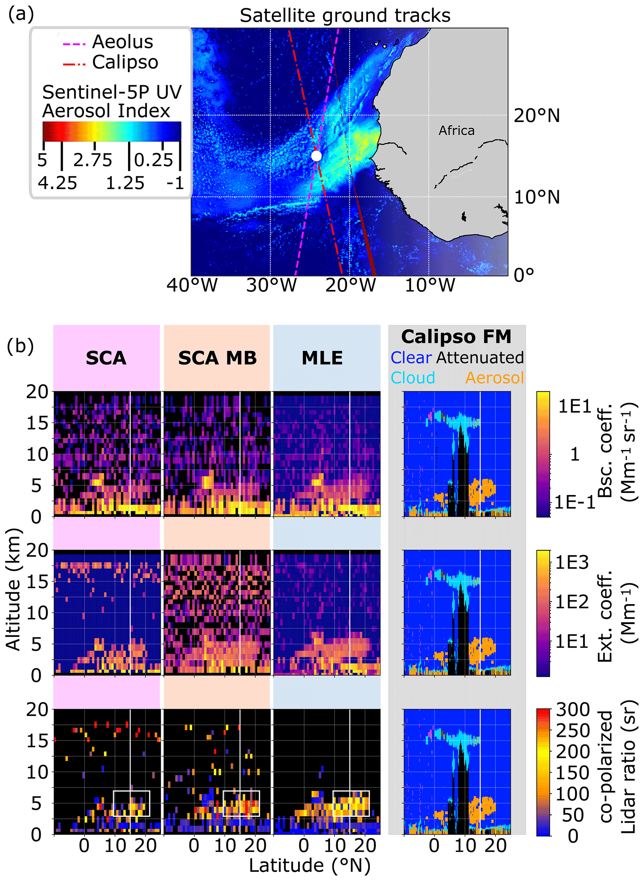
Figure 6Real data case I: (a) map of Africa's east coast overlaid with the ground tracks of the Aeolus satellite between 07:30 and 07:40 UTC (pink, dashed) and the CALIPSO satellite between 15:20 and 15:30 UTC (red, dash-dotted). Overlaid in colour is the Sentinel-5p UV aerosol index from 388 and 354 nm spectral bands. (b) Optical property processing results for the extended desert dust plume (Saharan Air Layer, SAL) from 30 June 2020 for the different algorithms. Columns in panel (b) (from left to right) are the SCA, SCA midbin and MLE. The rows show backscatter (first row), extinction (second row) and lidar ratio (last row). The CALIPSO vertical feature mask (VFM) is repeated in each row. Aeolus and CALIPSO ground tracks cross at the white line. For better interpretability, the lidar ratio is only shown where the corresponding backscatter coefficients exceed 0.25 Mm−1 sr−1, and extinction coefficients exceed 3.75 Mm−1.
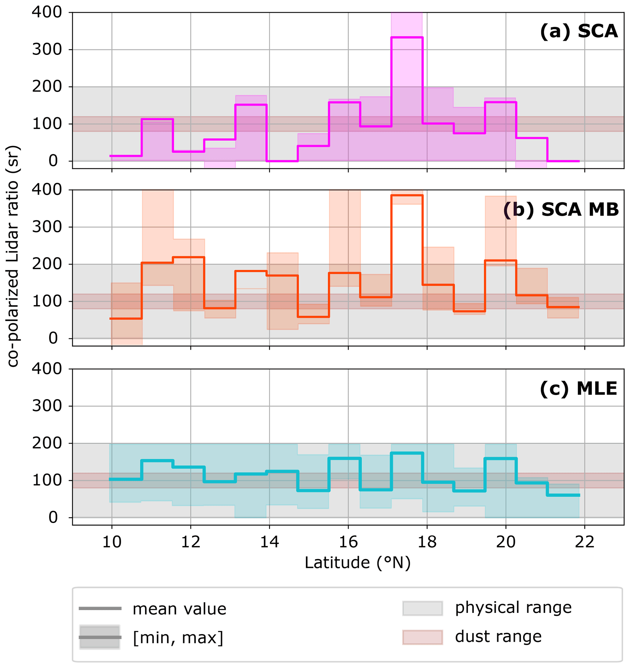
Figure 7Real data case I: averaged co-polarized lidar ratios according to along the Aeolus ground track, calculated from the 4×15 bins (altitude × latitude) within the white box in Fig. 6. Applied algorithms (from top to bottom) are (a) the SCA, (b) the midbin and (c) MLE. The shaded colours indicate the range between minimum and maximum lidar ratios for all considered bins in the column. Additionally, the expected range for the co-polarized lidar ratio of dust is indicated in shaded brown.
The SCA, SCA midbin and MLE processing results for backscatter, extinction and lidar ratio at a horizontal resolution of one BRC ≈87 km along-track distance are shown together with CALIPSO vertical feature mask (VFM) results in Fig. 6b. The afternoon CALIPSO VFM results show a partly lofted aerosol plume that is classified as desert dust in the latitude band 10 to 20∘ N, which also compares well with the TROPOMI observations in Fig. 6a. The area towards the Equator is partly attenuated by a high ice cloud between 10 and 16 km altitude, which was possibly on top of a convective cloud tower. The dust plume likely extended below as more dust is reported by the CALIPSO VFM close to the Equator. In the planetary boundary layer (PBL) low, broken clouds are visible in the FM. Additionally, patches of clouds are visible, e.g. at about 5 to 6 km height and 5∘ N. The optical property processing results of the Aeolus signals show similar features, except for the high cloud, which was not present during the Aeolus morning overpass. It should also be noted that convective activity is low in the morning and at its maximum in the early afternoon. Pronounced background noise patterns are present in SCA and SCA midbin backscatter coefficients (noise magnitude about 1 Mm−1 sr−1) and extinction coefficients (noise magnitude about 30 Mm−1), very similarly to the simulation cases I and II. Therefore, the SCA and SCA midbin show the dust plume only with little contrast and disrupted by noise. What is likely cloud is visible by a high return signal (yellow spots in backscatter) and low lidar ratios (dark blue colour). In these bins with a high signal-to-noise ratio, the SCA and MLE give very similar results, as expected. The SCA midbin suffers from the lower vertical resolution and significantly enhances the cloud and aerosol plume layer thickness, both in the PBL and at about 5 km height, but reconstructs fairly homogeneous extinction coefficients where the plume is located. Much higher contrast to the background is achieved with MLE, so the plume top and plume bottom heights can be inferred along the latitude. The plume detected by Aeolus algorithms agrees well with the CALIPSO VFM results despite Aeolus' coarse resolution and possible representation errors due to the difference in time and space between the observations by the two satellites. Only MLE captures the partly lofted nature of the plume north of the co-location point (white line). Furthermore, MLE achieves more homogeneous results along track for all properties, which demonstrates the advantage of the box constraints because no such smoothness constraint has yet contributed to the reconstruction.
Care has been taken in determination of the co-polarized lidar ratio of the dust in Fig. 7. All bins that lie within the white rectangle in Fig. 6b have been considered for the estimates due to the fairly homogeneous appearance in MLE and CALIPSO VFM. It is not reasonable to directly average the co-polarized lidar ratio over all bins as our convention would bias the result: often, the cross-polarized backscatter-to-extinction ratio (BER) is reported instead, but different conventions produce different results because , with mean 〈…〉. Hence, we first average backscatter and extinction coefficients over the box and report an unambiguous value for co-polarized lidar ratio, namely
that can be transformed into cross-polarized BER. The results read 78 sr for SCA, 120 sr for SCA midbin and 104 sr for MLE, which are in line with the expected values of co-polarized lidar ratio of 80 to 120 sr for depolarizing desert dust (Wandinger et al., 2015). This expected range is additionally visualized in Fig. 7, which illustrates the noise-induced variability in the lidar ratio along the plume's horizontal extent: the standard approaches SCA and SCA midbin fail to indicate a coherent feature along track by means of lidar ratio. The estimates range from 0 to 320 and 50 to 370 sr, respectively, although the results have been averaged over 4 km altitude, i.e. four range bins in this case. The MLE achieves the most coherent results along the SAL, with estimates between 60 and 170 sr. In combination with the curtain plots in Fig. 6, this demonstrates that the presented MLE approach allows for more robust aerosol classification than the SCA and SCA MB based on the lidar ratio estimates.
4.4 Real data case II: ground-based validation
On 9 November 2019, Aeolus passed close to a ground-based, remote-controlled multiwavelength-polarization Raman lidar (Polly) in Tel Aviv at 03:50 UTC, which is part of PollyNET (Baars et al., 2016; Engelmann et al., 2016). This network consists of several such automated Polly lidars for automated and continuous 24/7 observations of clouds and aerosols around the world. As such, they can also provide vital input for calibration and validation activities of Aeolus' optical property observations. The ground-based lidar data in Fig. 8 have been accumulated over the time 02:41 to 03:40 UTC. The distance to the centres of the two closest Aeolus observations (which are 87 km averages along the satellite orbit) are 68 and 84 km. A special range bin setting is operational in this area: the altitude range between 2 and 4 km is divided into eight range bins of 250 m width to detect lofted dust at the highest possible instrument resolution. Thus, the SNR in this layer is smaller than usual, which provides a challenging test case for validation of MLE against the standard approaches. The atmospheric scene was characterized by a temporally stable aerosol layering. For the entire night over Tel Aviv, a PBL with high backscatter values (3–6 Mm−1) up to 1 km was observed, while above, moderate backscattering (about 2 Mm−1) up to 3.5 km was present. According to the PollyNET target categorization (Baars et al., 2017), both layers were identified as a mix of pollution and dust with particle linear depolarization ratio values of about 10 % and co-polarized lidar ratio values between 40 and 50 sr (at 355 nm).
The optical properties from the SCA, SCA midbin and MLE processing are overlaid in Fig. 8. The results of backscatter coefficients appear disrupted by noise for the SCA and SCA midbin; that is, negative or missing values are present in all profiles within the aerosol layer below 3.5 km but for MLE processing. By comparison to the similar simulation case I, we expect a backscatter coefficient error in MLE retrieval on the order of 30 % within the aerosol layer below 3.5 km and an extinction coefficient error on the order of 100 % for individual range bins. A comparison of SCA and SCA MB results with the simulation case I and the ground truth also suggests that the currently reported error in the L2A product is no reliable estimate. The MLE is also able to retrieve the vertically coherent aerosol layer in good agreement with the ground truth (Raman method at 355 nm; Ansmann et al., 1992). Additionally, MLE results for both independent Aeolus observations agree well with each other and show much lower variability than the SCA and SCA midbin results. All aspects considered, the good agreement with the ground case and the consistent retrieval in both neighbouring columns are strong indicators that the MLE successfully suppressed noise.
The extinction retrieval is challenged by the lowered SNR in the fine vertical range bin setting, but MLE achieves the most reasonable results closest to the ground truth and suppresses outliers above 3.5 km. After all, the coherent aerosol layer cannot be located by using extinction coefficients alone due to the fine range bin settings between 2 and 4 km that cause high noise amplitudes. Still, the averaged co-polarized lidar ratio is calculated from the altitude range 1.5 to 3.5 km and both observations, as suggested in Eq. (16). The results read (75±98) sr for SCA, (73±31) sr for SCA midbin and 51 sr for MLE, so MLE retrieves the most accurate result compared to the ground truth value between 40 and 50 sr, though the sensitivity of these results to calibration errors has not been considered.
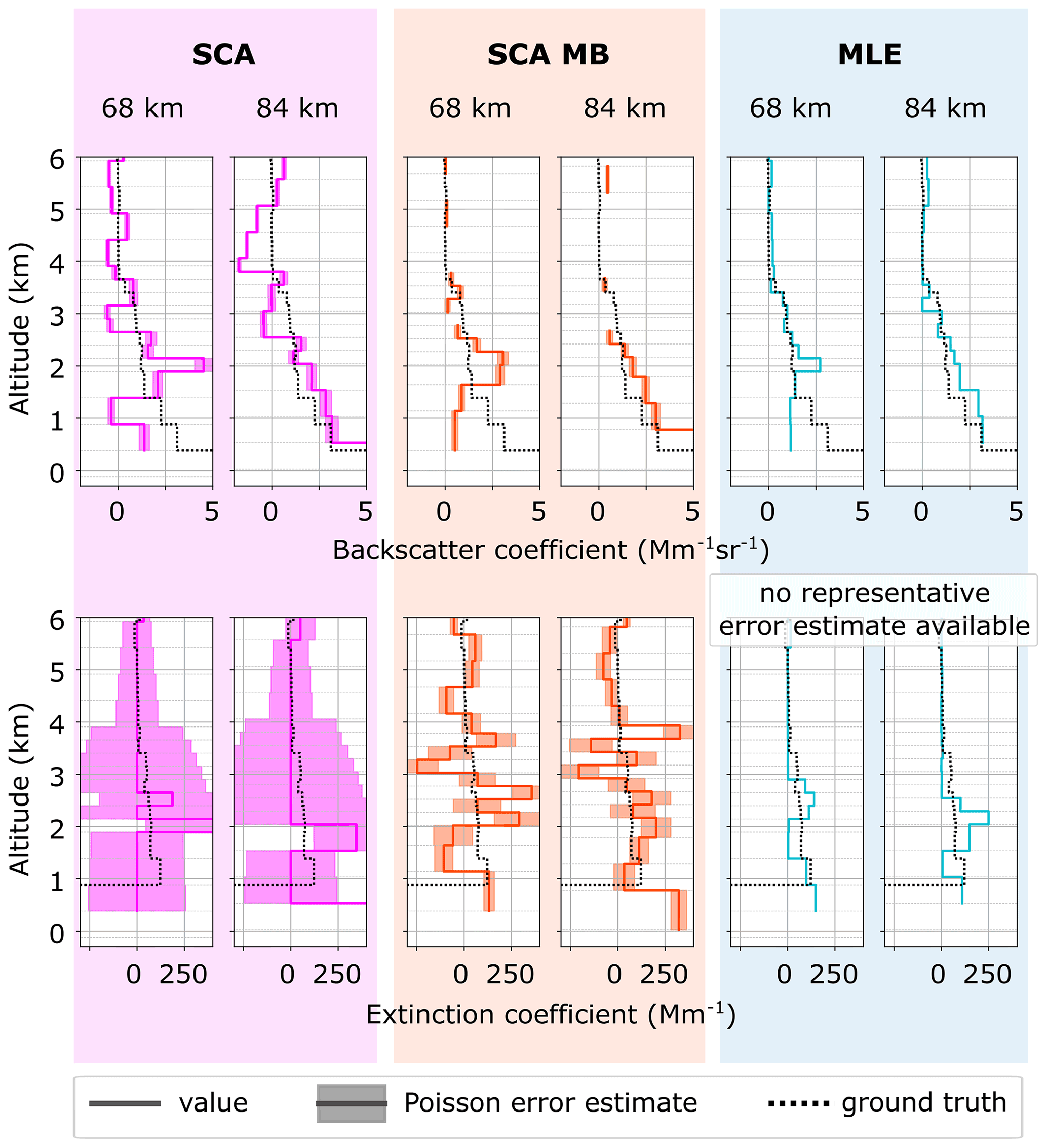
Figure 8Real data case II: optical properties of two co-located Aeolus observations (solid coloured lines) compared to the ground truth observations over Tel Aviv (solid black lines). The ground truth co-polarized backscatter and extinction have been binned to Aeolus resolution. Applied algorithms (from left to right) are the SCA, SCA midbin and MLE. Distances between the ground station and the centre of Aeolus observation are 68 and 84 km. The error bounds from Poisson assumptions are displayed in shaded colours.
The optical property retrieval within the Aeolus Level 2A aerosol optical property data product has been reformulated as a MLE problem and was successfully implemented and tested. The evaluation of the new MLE retrieval revealed a predominantly positive impact: it is demonstrated that the precision of the MLE outperforms the SCA and SCA midbin in synthetic homogeneous scenes and, additionally, reduces biases in the mean statistics. Furthermore, these trends have been confirmed in two cases of real Aeolus data. All cases consistently indicate that MLE is particularly advantageous for estimation of extinction coefficients and co-polarized lidar ratios. However, the precision of co-polarized backscatter coefficients increased overall as well by application of MLE. The coupled retrieval of all aerosol optical properties (extinction, backscatter and lidar ratio) is in line with the work of Povey et al. (2014) and distinct from the approaches described in Shcherbakov (2007), Marais et al. (2016) and Xiao et al. (2020). A retrieval that implements constraints within the simultaneous retrieval of backscatter and extinction improves precision. The improvements of the MLE are due to the introduction of positivity and lidar ratio constraints that force particle extinction to appear only where there is particle backscatter along the atmospheric column and vice versa. Since the box constraints are integral to the simultaneous retrieval of backscatter and extinction, noise is suppressed in both products simultaneously in contrast to the zero-flooring of the SCA, which considers the extinction variable independently without regard to the fact that the signal errors are correlated due to channel crosstalk correction (Appendix A). Furthermore, the results of the SCA and SCA MB do not strictly fall into a physically meaningful subset of solutions; e.g. they include negative backscatter coefficients. It is important to note that despite the improvements, moderate backscatter coefficients of about 0.1 Mm−1 sr−1 can still not be distinguished from zero on a single-bin basis. Higher precision can only be achieved by signal accumulation or averaging of the backscatter coefficient estimates.
A remaining shortcoming of the SCA and MLE algorithms is the signal accumulation at coarse horizontal scales of 87 km, although measurements are principally available at 3 km horizontal resolution. If the SNR was sufficient, the MLE could be applied at finer scales as the horizontal resolution alters only the number of atmospheric profiles within the minimization problem (see Eq. 15). In order to guarantee a sufficient SNR, it is possible to include a feature mask in the processing chain. With this, the MLE could be performed on distinct features with sufficient signal accumulation. But any attempt to create a feature mask from the lidar signals itself is flawed because even a homogeneous patch of atmosphere can appear inhomogeneous (in the signals) when parts of the profiles have been attenuated above. Therefore, in order to estimate aerosol optical properties at finer scales, it is more elegant to apply a suitable regularization within the retrieval problem itself, i.e. to add an additional regularization term in the cost function (see Eq. 15). Shcherbakov (2007) applied a Tikhonov smoothness constraint in the vertical direction but stressed the need for a regularization that favours piecewise constant functions. Marais et al. (2016) and Xiao et al. (2020) have therefore made use of the total variation regularization in HSRL lidar ratio retrieval along both horizontal and vertical directions. This is particularly useful to retrieve piecewise constant functions and is hence the optimal choice for the lidar ratio variable when the atmosphere is assumed to consist of patches of the same aerosol species. In summary, such regularization is principally able to merge (i) the problem of defining a feature mask from raw lidar data and (ii) the optical property retrieval in low-SNR conditions. Eventually, we propose to extend the current MLE approach by a total variation regularization term in order to enable robust optical property retrievals with Aeolus at finer scales. This could be attempted in future versions of the MLE algorithm. Additionally, a proper implementation of the box constraints in the uncertainty estimation is lacking so far, which requires future investigation.
All details of the SCA are thoroughly described in the algorithm theoretical baseline document of the L2A processor (Flamant et al., 2020), but this section briefly recaps the main steps and discusses the shortcomings of the SCA. In the following, the index as subscript to the properties in Sect. 3 denotes the range bin index. This implies for the signals s, X and Y that the property has been integrated over a discrete range , i.e. . For all other variables like backscatter coefficients β, extinction coefficients α and range R, this subscript denotes the average in range bin i, i.e. , with , and equivalently for subscript m. As a consequence, particle optical depth of a bin is denoted , and the particle one-way transmission becomes
with unknown optical depth Lp,sat in between the telescope and first range bin. The following approximations for the range-corrected signals (Eqs. 5 and 6) are made by using the mean bin properties from above (see Eqs. 6.35–6.36 and definitions above in Flamant et al., 2020):
With this, Eqs. (7) and (8) can be rephrased to
This way, the signals in the Rayleigh and Mie channels are expressed as functions of aerosol optical property proxies and Lp,i (and Lp,sat) solely, which are equivalent to αp,i and (and Lp,sat). Temperature, pressure and Doppler shift (due to horizontal-line-of-sight wind) are assumed known a priori by means of ECMWF medium-range weather forecasting. Hence, the molecular optical properties, i.e. all variables with subscript m, can be inferred with sufficient accuracy as well. The standard SCA solves Eqs. (A2) to (A5) exactly in a recursive scheme beginning with default initial conditions in the first range bin to correct for non-zero optical depth above the measurement volume. More precisely, backscatter is calculated directly from
And layer optical depth is retrieved independently from the profile of Xi. Afterwards, the slant optical depth is transformed into the nadir optical depth by a trigonometric correction factor, from which extinction is directly calculated.
But the SCA suffers from several shortcomings. Any input data are assumed noise-free, and an exact solution of the extinction retrieval problem is calculated. Among the former strategies to dampen the noise within the SCA are averaged extinction estimates over vertically neighbouring range gates, which are called midbin properties (Sect. 6.3 in Flamant et al., 2020), and zero-flooring (Sect. 6.2.2.1 in Flamant et al., 2020) whenever negative extinction values would be obtained in the regular case. These SCA midbin properties are also denoted by the SCA MB in this work. Both strategies are ad hoc, but averaging is believed to introduce less bias than flooring because noise is cut off only in one direction by the latter. Furthermore, the signal noise amplitude can change abruptly from one range bin to another due to the varying vertical range bin heights (250 m to 2 km). Hence, since this varying reliability of the signals is not taken into account, biases or oscillations in the extinction variable can potentially be triggered by zero-flooring whenever range bin heights change. This is due to the fact that extinction essentially depends on the moving ratio of noisy signal values along an atmospheric column. The mean absolute of this ratio increases with increasing noise, which may then lead to a bias after zero-flooring negative values in the SCA (see also Flament et al., 2021, for a graphical explanation and a showcase without flooring). Additionally, extinction is retrieved independently from backscatter after the linear equation system in Eqs. (A4) and (A5) has been solved via standard methods. But due to the linear transform, the errors in properties Xi and Yi are found to be highly anti-correlated. To illustrate this, one can solve Eqs. (A4) and (A5) to obtain from error propagation that
with noise terms ε and rescaled coefficients . Accordingly, the noise from the Mie and Rayleigh channels contributes to the noise in Xi and Yi with alternating signs so that the negative cross-correlation is obtained. This means, for example, that one noisy value in the Mie (or Rayleigh) channel disturbs both backscatter and extinction coefficients. That also implies that if an unphysical, negative value is obtained in one bin for backscatter (or extinction) in the final result, then the value for extinction (or backscatter) is definitely disturbed as well, whether it lies within physical bounds or not. This additional knowledge is not accounted for within the processing, and hence low SNR in one of the signal channels has the potential to deteriorate both backscatter and extinction estimates. For example, the contribution from the Mie channel in a particle-free atmosphere is more than half noise, which affects the crosstalk-corrected molecular signal X and consequently the extinction retrieval as well.
The lidar data at a 2.9 km measurement scale (indexed m) within an observation are horizontally accumulated at an observation scale of 87 km before the analysis; i.e.
In the case that the scene is truly homogeneous, sm has the same mean and standard deviation . Then, a more robust estimate of the signal uncertainty can be provided from error propagation
and σconst can be estimated from the variance of the 30 signal values at the measurement scale, namely
This estimate will cover all additionally known and unknown noise sources and coincides with the Poisson noise hypothesis in the case that the measurement-scale signals are truly Poisson-distributed. The measurement error covariance Sy comprises the terms for both channels, Mie and Rayleigh, and all range bins on its diagonal.
The software code of the full L2A processor is not publicly available. The developed procedure and plugin for MLE processing can be shared upon request to the corresponding author. Data that were used to compile the plots can be shared upon request as well.
FE is the main author of this paper. He has developed the MLE implementation and has tested it together with the SCAs on the test datasets presented here. He has also performed the scientific analysis. The colleagues at Météo-France have developed the Aeolus L2A algorithms and are currently maintaining the L2A processor including important calibration updates and analyses. As such, TF, AD, DT and AL have supported with many fruitful discussions about Aeolus' calibration procedures and noise characterization. AL provided the end-to-end simulations. HB has provided the ground truth lidar data and reviewed this paper. AGSL has defined the tasks and work plan for this project and has supervised FE during his German traineeship at ESA. She has also reviewed this paper.
The contact author has declared that neither they nor their co-authors have any competing interests.
The presented work includes preliminary data (not fully calibrated or validated and not yet publicly released) of the Aeolus mission, which is part of the European Space Agency (ESA) Earth Explorer Programme. This includes wind products from before the public data release in May 2020 and/or aerosol and cloud products which have not yet been publicly released. The preliminary Aeolus wind products will be reprocessed during 2020 and 2021, which will include in particular a significant L2B product wind bias reduction and improved L2A radiometric calibration. Aerosol and cloud products became publicly available in June 2021. The processor development, improvement and product reprocessing preparation are performed by the Aeolus DISC (Data, Innovation and Science Cluster), which involves DLR, DoRIT, ECMWF, KNMI, CNRS, S&T, ABB and Serco, in close cooperation with the Aeolus PDGS (Payload Data Ground Segment). The analysis has been performed in the framework of the Aeolus Data Innovation and Science Cluster (Aeolus DISC).
Publisher’s note: Copernicus Publications remains neutral with regard to jurisdictional claims in published maps and institutional affiliations.
This article is part of the special issue “Aeolus data and their application (AMT/ACP/WCD inter-journal SI)”. It is not associated with a conference.
The main author has performed this work in the framework of his German traineeship at ESTEC, enabled and supported by the German Aerospace Center (DLR). His special thanks go to Anne Grete Straume-Lindner and Thorsten Fehr for their dedication and great personal support within extraordinary circumstances.
Parts of this research have been supported by the German Federal Ministry for Economic Affairs and Energy (BMWi) (grant no. 50EE1721C). The authors also received funding through ACTRIS-2 (grant no. 654109) from the European Union's Horizon 2020 research and innovation programme and through PoLiCyTa from the German Federal Ministry of Education and Research (BMBF) (grant no. 01LK1603A).
This paper was edited by Andrew Sayer and reviewed by three anonymous referees.
Ansmann, A., Wandinger, U., Riebesell, M., Weitkamp, C., and Michaelis, W.: Independent measurement of extinction and backscatter profiles in cirrus clouds by using a combined Raman elastic-backscatter lidar, Appl. Optics, 31, 7113–7131, https://doi.org/10.1364/AO.31.007113, 1992. a
Ansmann, A., Wandinger, U., Rille, O. L., Lajas, D., and Straume, A. G.: Particle backscatter and extinction profiling with the spaceborne high-spectral-resolution Doppler lidar ALADIN: methodology and simulations, Appl. Optics, 46, 6606–6622, https://doi.org/10.1364/AO.46.006606, 2007. a, b, c, d
Baars, H., Kanitz, T., Engelmann, R., Althausen, D., Heese, B., Komppula, M., Preißler, J., Tesche, M., Ansmann, A., Wandinger, U., Lim, J.-H., Ahn, J. Y., Stachlewska, I. S., Amiridis, V., Marinou, E., Seifert, P., Hofer, J., Skupin, A., Schneider, F., Bohlmann, S., Foth, A., Bley, S., Pfüller, A., Giannakaki, E., Lihavainen, H., Viisanen, Y., Hooda, R. K., Pereira, S. N., Bortoli, D., Wagner, F., Mattis, I., Janicka, L., Markowicz, K. M., Achtert, P., Artaxo, P., Pauliquevis, T., Souza, R. A. F., Sharma, V. P., van Zyl, P. G., Beukes, J. P., Sun, J., Rohwer, E. G., Deng, R., Mamouri, R.-E., and Zamorano, F.: An overview of the first decade of PollyNET: an emerging network of automated Raman-polarization lidars for continuous aerosol profiling, Atmos. Chem. Phys., 16, 5111–5137, https://doi.org/10.5194/acp-16-5111-2016, 2016. a
Baars, H., Seifert, P., Engelmann, R., and Wandinger, U.: Target categorization of aerosol and clouds by continuous multiwavelength-polarization lidar measurements, Atmos. Meas. Tech., 10, 3175–3201, https://doi.org/10.5194/amt-10-3175-2017, 2017. a
Chanin, M. L., Garnier, A., Hauchecorne, A., and Porteneuve, J.: A Doppler lidar for measuring winds in the middle atmosphere, Geophys. Res. Lett., 16, 1273–1276, https://doi.org/10.1029/GL016i011p01273, 1989. a
Dabas, A.: Generation of AUX CAL Detailed Processing Model Input Output data definition, ESA, available at: https://earth.esa.int/eogateway/documents/20142/37627/Aeolus-AUX-CAL-IODD-DPM.pdf (last access: 3 January 2022), 2017. a
Denevi, G., Garbarino, S., and Sorrentino, A.: Iterative algorithms for a non-linear inverse problem in atmospheric lidar, Inverse Probl., 33, 085010, https://doi.org/10.1088/1361-6420/aa7904, 2017. a, b, c, d
Donovan, D. P., van Zadelhoff, G.-J., Williams, J. E., Wandinger, U., Haarig, M., and Qu, Z.: Development of ATLID Retrieval Algorithms, EPJ Web Conf., 237, 01005, https://doi.org/10.1051/epjconf/202023701005, 2020. a
Eloranta, E.: High Spectral Resolution lidar measurements of atmospheric extinction: Progress and challenges, in: 2014 IEEE Aerospace Conference, Big Sky, MT, USA, 1-8 March 2014, 1–6, https://doi.org/10.1109/AERO.2014.6836214, 2014. a
Engelmann, R., Kanitz, T., Baars, H., Heese, B., Althausen, D., Skupin, A., Wandinger, U., Komppula, M., Stachlewska, I. S., Amiridis, V., Marinou, E., Mattis, I., Linné, H., and Ansmann, A.: The automated multiwavelength Raman polarization and water-vapor lidar PollyXT: the neXT generation, Atmos. Meas. Tech., 9, 1767–1784, https://doi.org/10.5194/amt-9-1767-2016, 2016. a
ESA: ADM-Aeolus Science Report ESA SP-1311, ESA Communication Production Office, available at: https://esamultimedia.esa.int/multimedia/publications/SP-1311/SP-1311.pdf (last access: 3 January 2022), 2008. a, b
ESA: TROPOMI Level 2 Ultraviolet Aerosol Index products, Version 01, Copernicus Sentinel-5P, ESA [data set], https://doi.org/10.5270/S5P-0wafvaf, 2018. a
Fernald, F. G.: Analysis of atmospheric lidar observations: some comments, Appl. Optics, 23, 652–653, https://doi.org/10.1364/AO.23.000652, 1984. a
Flamant, P., Cuesta, J., Denneulin, M.-L., Dabas, A., and Huber, D.: ADM-Aeolus retrieval algorithms for aerosol and cloud products, Tellus A, 60, 273–288, https://doi.org/10.1111/j.1600-0870.2007.00287.x, 2008. a, b
Flamant, P., Lever, V., Martinet, P., Flament, T., Cuesta, J., Dabas, A., Olivier, M., and Huber, D.: ADM-Aeolus L2A Algorithm Theoretical Baseline Document, ESA, available at: https://earth.esa.int/eogateway/documents/20142/37627/Aeolus-L2A-Algorithm-Theoretical-Baseline-Document (last access: 3 January 2022), 2020. a, b, c, d, e, f, g, h, i, j, k, l, m, n, o
Flament, T., Trapon, D., Lacour, A., Dabas, A., Ehlers, F., and Huber, D.: Aeolus L2A Aerosol Optical Properties Product: Standard Correct Algorithm and Mie Correct Algorithm, Atmos. Meas. Tech. Discuss. [preprint], https://doi.org/10.5194/amt-2021-181, in review, 2021. a, b, c
Garbarino, S., Sorrentino, A., Massone, A. M., Sannino, A., Boselli, A., Wang, X., Spinelli, N., and Piana, M.: Expectation maximization and the retrieval of the atmospheric extinction coefficients by inversion of Raman lidar data, Opt. Express, 24, 21497–21511, https://doi.org/10.1364/OE.24.021497, 2016. a, b, c, d
Garnier, A. and Chanin, M. L.: Description of a Doppler Rayleigh LIDAR for measuring winds in the middle atmosphere, Appl. Phys. B, 55, 35–40, https://doi.org/10.1007/BF00348610, 1992. a
Gentry, B. M., Chen, H., and Li, S. X.: Wind measurements with 355-nm molecular Doppler lidar, Opt. Lett., 25, 1231–1233, https://doi.org/10.1364/OL.25.001231, 2000. a
Grund, C. J. and Eloranta, E. W.: Fiber-optic scrambler reduces the bandpass range dependence of Fabry–Perot étalons used for spectral analysis of lidar backscatter, Appl. Optics, 30, 2668–2670, https://doi.org/10.1364/AO.30.002668, 1991. a
Illingworth, A. J., Barker, H. W., Beljaars, A., Ceccaldi, M., Chepfer, H., Clerbaux, N., Cole, J., Delanoë, J., Domenech, C., Donovan, D. P., Fukuda, S., Hirakata, M., Hogan, R. J., Huenerbein, A., Kollias, P., Kubota, T., Nakajima, T., Nakajima, T. Y., Nishizawa, T., Ohno, Y., Okamoto, H., Oki, R., Sato, K., Satoh, M., Shephard, M. W., Velázquez-Blázquez, A., Wandinger, U., Wehr, T., and van Zadelhoff, G.-J.: The EarthCARE Satellite: The Next Step Forward in Global Measurements of Clouds, Aerosols, Precipitation, and Radiation, B. Am. Meteorol. Soc., 96, 1311–1332, https://doi.org/10.1175/BAMS-D-12-00227.1, 2015. a, b, c, d
IPCC: Climate Change 2013: The Physical Science Basis. Contribution of Working Group I to the Fifth Assessment Report of the Intergovernmental Panel on Climate Change, Cambridge University Press, Cambridge, United Kingdom and New York, NY, USA, https://doi.org/10.1017/CBO9781107415324, 2013. a
Klett, J. D.: Stable analytical inversion solution for processing lidar returns, Appl. Optics, 20, 211–220, https://doi.org/10.1364/AO.20.000211, 1981. a
Korb, C. L., Gentry, B. M., and Weng, C. Y.: Edge technique: theory and application to the lidar measurement of atmospheric wind, Appl. Optics, 31, 4202–4213, https://doi.org/10.1364/AO.31.004202, 1992. a
Marais, W. J., Holz, R. E., Hu, Y. H., Kuehn, R. E., Eloranta, E. E., and Willett, R. M.: Approach to simultaneously denoise and invert backscatter and extinction from photon-limited atmospheric lidar observations, Appl. Optics, 55, 8316–8334, https://doi.org/10.1364/AO.55.008316, 2016. a, b, c, d, e, f, g
Martino, A. J., Neumann, T. A., Kurtz, N. T., and McLennan, D.: ICESat-2 mission overview and early performance, in: Sensors, Systems, and Next-Generation Satellites XXIII, edited by: Neeck, S. P., Martimort, P., and Kimura, T., International Society for Optics and Photonics, SPIE, 11151, 68–77, https://doi.org/10.1117/12.2534938, 2019. a
McGill, M. J., Yorks, J. E., Scott, V. S., Kupchock, A. W., and Selmer, P. A.: The Cloud-Aerosol Transport System (CATS): a technology demonstration on the International Space Station, in: Lidar Remote Sensing for Environmental Monitoring XV, edited by: Singh, U. N., International Society for Optics and Photonics, SPIE, 9612, 34–39, https://doi.org/10.1117/12.2190841, 2015. a
Pappalardo, G., Amodeo, A., Apituley, A., Comeron, A., Freudenthaler, V., Linné, H., Ansmann, A., Bösenberg, J., D'Amico, G., Mattis, I., Mona, L., Wandinger, U., Amiridis, V., Alados-Arboledas, L., Nicolae, D., and Wiegner, M.: EARLINET: towards an advanced sustainable European aerosol lidar network, Atmos. Meas. Tech., 7, 2389–2409, https://doi.org/10.5194/amt-7-2389-2014, 2014. a
Pornsawad, P., Böckmann, C., Ritter, C., and Rafler, M.: Ill-posed retrieval of aerosol extinction coefficient profiles from Raman lidar data by regularization, Appl. Optics, 47, 1649–1661, https://doi.org/10.1364/AO.47.001649, 2008. a, b
Pornsawad, P., D'Amico, G., Böckmann, C., Amodeo, A., and Pappalardo, G.: Retrieval of aerosol extinction coefficient profiles from Raman lidar data by inversion method, Appl. Optics, 51, 2035–2044, https://doi.org/10.1364/AO.51.002035, 2012. a, b
Povey, A. C., Grainger, R. G., Peters, D. M., and Agnew, J. L.: Retrieval of aerosol backscatter, extinction, and lidar ratio from Raman lidar with optimal estimation, Atmos. Meas. Tech., 7, 757–776, https://doi.org/10.5194/amt-7-757-2014, 2014. a, b, c, d
Prospero, J. M. and Carlson, T. N.: Saharan air outbreaks over the tropical North Atlantic, Pure Appl. Geophys., 119, 677–691, https://doi.org/10.1007/BF00878167, 1980. a
Reitebuch, O., Huber, D., and Nikolaus, I.: ADM-Aeolus Algorithm Theoretical Basis Document ATBD Level1B Products, ESA, available at: https://earth.esa.int/eogateway/documents/20142/37627/Aeolus-L1B-Algorithm-ATBD.pdf (last access: 3 January 2022), 2018a. a, b, c, d, e
Reitebuch, O., Marksteiner, U., Rompel, M., Meringer, M., Schmidt, K., Huber, D., Nikolaus, I., Dabas, A., Marshall, J., de Bruin, F., Kanitz, T., and Straume, A.-G.: Aeolus End-To-End Simulator and Wind Retrieval Algorithms up to Level 1B, EPJ Web Conf., 176, 02010, https://doi.org/10.1051/epjconf/201817602010, 2018b. a
Reitebuch, O., Lemmerz, C., Lux, O., Marksteiner, U., Rahm, S., Weiler, F., Witschas, B., Meringer, M., Schmidt, K., Huber, D., Nikolaus, I., Geiss, A., Vaughan, M., Dabas, A., Flament, T., Stieglitz, H., Isaksen, L., Rennie, M., de Kloe, J., Marseille, G.-J., Stoffelen, A., Wernham, D., Kanitz, T., Straume, A.-G., Fehr, T., von Bismarck, J., Floberghagen, R., and Parrinello, T.: Initial Assessment of the Performance of the First Wind Lidar in Space on Aeolus, EPJ Web Conf., 237, 01010, https://doi.org/10.1051/epjconf/202023701010, 2020. a, b
Rodgers, C. D.: Inverse Methods for Atmospheric Sounding, World Scientific, Singapore, https://doi.org/10.1142/3171, 2000. a, b, c, d
Shcherbakov, V.: Regularized algorithm for Raman lidar data processing, Appl. Optics, 46, 4879–4889, https://doi.org/10.1364/AO.46.004879, 2007. a, b, c, d, e, f
She, C. Y., Alvarez, R. J., Caldwell, L. M., and Krueger, D. A.: High-spectral-resolution Rayleigh–Mie lidar measurement of aerosol and atmospheric profiles, Opt. Lett., 17, 541–543, https://doi.org/10.1364/OL.17.000541, 1992. a
Shimizu, H., Lee, S. A., and She, C. Y.: High spectral resolution lidar system with atomic blocking filters for measuring atmospheric parameters, Appl. Optics, 22, 1373–1381, https://doi.org/10.1364/AO.22.001373, 1983. a
Shipley, S. T., Tracy, D. H., Eloranta, E. W., Trauger, J. T., Sroga, J. T., Roesler, F. L., and Weinman, J. A.: High spectral resolution lidar to measure optical scattering properties of atmospheric aerosols. 1: Theory and instrumentation, Appl. Optics, 22, 3716–3724, https://doi.org/10.1364/AO.22.003716, 1983. a
Sica, R. J. and Haefele, A.: Retrieval of temperature from a multiple-channel Rayleigh-scatter lidar using an optimal estimation method, Appl. Optics, 54, 1872–1889, https://doi.org/10.1364/AO.54.001872, 2015. a
Souprayen, C., Garnier, A., and Hertzog, A.: Rayleigh–Mie Doppler wind lidar for atmospheric measurements. II. Mie scattering effect, theory, and calibration, Appl. Optics, 38, 2422–2431, https://doi.org/10.1364/AO.38.002422, 1999a. a
Souprayen, C., Garnier, A., Hertzog, A., Hauchecorne, A., and Porteneuve, J.: Rayleigh–Mie Doppler wind lidar for atmospheric measurements. I. Instrumental setup, validation, and first climatological results, Appl. Optics, 38, 2410–2421, https://doi.org/10.1364/AO.38.002410, 1999b. a
Spinhirne, J. D., Palm, S. P., Hart, W. D., Hlavka, D. L., and Welton, E. J.: Cloud and aerosol measurements from GLAS: Overview and initial results, Geophys. Res. Lett., 32, L22S03, https://doi.org/10.1029/2005GL023507, 2005. a
Stoffelen, A., Pailleux, J., Källén, E., Vaughan, J. M., Isaksen, L., Flamant, P., Wergen, W., Andersson, E., Schyberg, H., Culoma, A., Meynart, R., Endemann, M., and Ingmann, P.: The atmospheric dynamics mission for global wind field measurements, B. Am. Meteorol. Soc., 86, 73–88, https://doi.org/10.1175/BAMS-86-1-73, 2005. a
Wandinger, U., Amiridis, V., Freudenthaler, V., Komppula, M., Kokkalis, P., Engelmann, R., Marinou, E., and Tsekeri, A.: Validation of ADM-Aeolus L2 aerosol and cloud products employing advanced ground-based lidar measurements (VADAM), in: ADM-Aeolus Science and CAL/VAL Workshop, ESA-ESRIN, Frascati, Italy, 10–13 February 2015, 2015. a, b, c
Weiler, F.: Bias correction using ground echoes for the airborne demonstrator of the wind lidar on the ADM-Aeolus mission, Master thesis, Faculty of Geo- and Atmospheric Sciences, University of Innsbruck, Austria, 2015. a
Weitkamp, C.: Lidar: Range-Resolved Optical Remote Sensing of the Atmosphere, Springer Series in Optical Sciences, Springer New York, 2006. a, b, c
Whiteman, D. N.: Application of statistical methods to the determination of slope in lidar data, Appl. Optics, 38, 3360–3369, https://doi.org/10.1364/AO.38.003360, 1999. a
Winker, D. M., Pelon, J. R., and McCormick, M. P.: CALIPSO mission: spaceborne lidar for observation of aerosols and clouds, in: Lidar Remote Sensing for Industry and Environment Monitoring III, edited by: Singh, U. N., Itabe, T., and Liu, Z., International Society for Optics and Photonics, SPIE, 4893, 1–11, https://doi.org/10.1117/12.466539, 2003. a, b
Xiao, D., Wang, N., Shen, X., Landulfo, E., Zhong, T., and Liu, D.: Development of ZJU High-Spectral-Resolution Lidar for Aerosol and Cloud: Extinction Retrieval, Remote Sens., 12, 3047, https://doi.org/10.3390/rs12183047, 2020. a, b, c, d, e, f, g
Young, S. A., Winker, D., Vaughan, M., Hu, Y., and Kuehn, R.: CALIOP Algorithm Theoretical Basis Document Part 4: Extinction Retrieval Algorithms, available at: https://www-calipso.larc.nasa.gov/resources/ (last access: 3 April 2021), 2008. a
Zhu, C., Byrd, R. H., Lu, P., and Nocedal, J.: Algorithm 778: L-BFGS-B: Fortran Subroutines for Large-Scale Bound-Constrained Optimization, ACM T. Math. Software [code], 23, 550–560, https://doi.org/10.1145/279232.279236, 1997. a
- Abstract
- Introduction
- Instrument
- Methods
- Results and discussion
- Conclusions
- Appendix A: Standard correct algorithm (SCA)
- Appendix B: Uncertainty estimates from measurement variability
- Code and data availability
- Author contributions
- Competing interests
- Disclaimer
- Special issue statement
- Acknowledgements
- Financial support
- Review statement
- References