Fill dynamics and sample mixing in the AirCore

The AirCore is a long coiled tube that acts as a “tape recorder” of the composition of air as it is slowly filled or flushed. When launched by balloon with one end of the tube open and the other closed, the initial fill air flows out during ascent as the outside air pressure drops. During descent atmospheric air flows back in. I describe how we can associate the position of an air parcel in the tube with the altitude it came from by modeling the dynamics of the fill process. The conditions that need to be satisfied for the model to be accurate are derived. The extent of the mixing of air parcels that enter at different times is calculated so that we know how many independent samples are in the tube upon landing and later when the AirCore is analyzed.

1 Introduction

When the AirCore is filling with atmospheric air coming in through the open end, the newly sampled air pushes the air that is already in the tube deeper into the tube while compressing it. This mode of sampling is entirely passive, relying on the pressure continuing to increase as the altitude becomes lower during descent. The AirCore could also be flushed by a pump without any need for pressure changes of the outside air that is being sampled. I conceived the idea of the AirCore in the late 1990s after we had found ∼100-year-old air, as indicated by the measured levels of CO₂ and CH₄, near the bottom of the firn layer at a depth of ∼90 m at the South Pole (Battle et al., 1996). The air was very old despite the fact that there was still open contact with the present-day atmosphere. Over distances of tens of meters or more, molecular diffusion is exceedingly slow! The root-mean-square (rms) molecular diffusion distance is X_rms=(2Dt)^0.5. D is diffusivity in air, which for CO₂ is 0.140 cm² s⁻¹ at 1 bar and 0 ^∘C, and t is time in seconds. After 1 year the rms diffusion distance for CO₂ in air would be ∼30 m, which would be the scale of spreading if there is no macroscopic air motion at all. In addition, diffusive mixing deep in the firn is significantly slower than in open air because the air path from the bottom of the firn to the atmosphere has many detours going through the pores that are still open.

With Jim Smith and Michael Hahn, two members of our group in those days, we verified that there is very little mixing along the length of the tube by pushing slugs of air from two different reference air cylinders, alternating between high and low CO₂, through a long coiled tube. We also stored air for several hours before analysis. It all looked good. Then we tried a balloon flight. In order to make the payload lighter, we switched from stainless-steel to aluminum tubing, because of our excellent experience with long-term gas storage in high-pressure aluminum cylinders. It did not work at all. The easily bendable tube was made of a soft aluminum alloy, very different from the high-pressure cylinders. We found that the tube consumed CO₂ very effectively. It was going to take more effort to make it successful, and we did not have much time to devote to it. So the project languished for several years until Anna Karion, Colm Sweeney, and Tim Newberger of our group at GML (Global Monitoring Laboratory) were able to pick it up again. At the urging of Sandy MacDonald, who was director of NOAA's Earth System Research Laboratory at the time, I applied for a patent in August 2006. He pointed out that there are people trolling the scientific literature, conference proceedings, etc. to find ideas that could be patented so that we might find ourselves having to pay somebody else to use our own idea. Instead, we wanted the AirCore to be freely useable (and improved) by everyone so that my patent (Tans, 2009) was intended to be a defensive action!

We realized that AirCore technology could become extremely useful for the validation of satellite retrievals of column-averaged mole fractions of greenhouse gases. The measurements of a gas sample captured by the AirCore are calibrated, but care has to be taken, as with all air samples in containers, that no artifacts are introduced by the container or by gas-handling procedures. In contrast, remote sensing estimates of greenhouse gases can in principle never be calibrated. Metrology, the science of measurement, defines what a calibration is. Using a measurement standard, one presents the measurement method with a known value, under controlled conditions, so that the measurement indication is related to a quantity value (paraphrased from Bureau International de Poids et Mesures, 2008). In the case of greenhouse gases in the atmosphere, the conditions cannot be controlled. In addition, we realized that the regular deployment of AirCores could be a cost-effective way to monitor and study an evolving atmospheric circulation as climate change progresses, as proposed by Fred Moore (Moore et al., 2014).

Developments of the AirCore by various groups have been described in other papers, for example by Wagenhäuser et al. (2021) and Membrive et al. (2017). However, there has been neither a comprehensive treatment of fill dynamics nor a detailed look at mixing, hence this paper.

2 The physical principle that makes the AirCore work – molecular diffusion

Diffusive mixing over large distances is exceedingly slow, but there is another use of diffusion. Flow inside the tube is laminar, which has maximum speed in the center and zero speed at the wall. With velocities that differ from zero to some finite value, why does laminar flow not “smear out” our tape recorder signal by mixing air parcels that came in at different times? Again, molecular diffusion comes to the rescue. Using the square root relationship above, if the inner radius of the tube is 0.3 cm, it takes a CO₂ molecule on average only 0.03 s (at 1 bar pressure) to diffuse from the wall to the radius where the velocity equals the average velocity inside the tube. Any molecule will be close to the wall, as well as near the center, of the tube many times per second. Therefore the speed of all molecules in the long direction of the tube, averaged over a few seconds, is very nearly the same. However, the AirCore idea does not work so well for liquids. In water the molecular diffusivity is ∼10 000 times lower than in air at 1 bar so that the smearing of a tape recorder signal could be very large. To compensate for such low diffusivity, both the diameter of the tube and the flow speed will have to be kept low, and there will also be capillary effects. Water may be attracted to or repelled by the tube wall, influencing the flow.

The AirCore collects a continuous sample. Instead of valves, distance in the tube is used to keep separated the air that has been sampled from different pressure altitudes. The number of independent samples (the inverse of vertical resolution) in the tube decreases as the time between collection and measurement becomes longer. The measurement or “readout” of the vertical profile is carried out by attaching an analytical instrument to one end of the tube and a cylinder with air of a well-known composition to the other end. The latter pushes the sampled air slowly through the analyzer. The procedure, as well as various tests of mixing, has been described by Anna Karion of GML (Karion et al., 2010).

3 Dynamics of the fill process

How do we accurately associate position in the tube with the geometric altitude or pressure altitude that the sample at that position came from? It is the first question we address in this paper. The filling does not occur uniformly as a function of pressure altitude. The second question is how far the mixing of adjacent air parcels extends as a result of molecular diffusion and secondarily as a result of the flow itself. It will be addressed in Sect. 6. I wrote the first version of the fill dynamics calculation to make the association of altitude with position in 2005, called rocketfall.pro, coded in Interactive Data Language (IDL). Undergraduate students in the engineering department at the University of Colorado were getting ready to put an AirCore on a NASA rocket, and I was worried about there not being enough time to passively collect air from the stratosphere as the rocket was falling at supersonic speeds. There have been several successive versions of the algorithm since then. The significantly improved IDL version of July 2021 is described in this paper.

We use a fluid dynamics model and a subset of the flight data, namely the time, pressure and temperature of outside air and the temperature of the tube, as input data. The starting point is Poiseuille's equation for steady-state laminar flow in a tube with a circular cross section:

$$\begin{array}{}\text{(1)}& Q_{\mathrm{m}}={\displaystyle \frac{-\mathit{\rho }\mathit{\pi }{r}^{\mathrm{4}}}{\mathrm{8}\mathit{\eta }}}{\displaystyle \frac{\mathrm{d}P}{\mathrm{d}z}}\text{or}{Q}_n={\displaystyle \frac{-{\mathit{\rho }}_n\mathit{\pi }{r}^{\mathrm{4}}}{\mathrm{8}\mathit{\eta }}}{\displaystyle \frac{\mathrm{d}P}{\mathrm{d}z}},\end{array}$$

in which Q_m is mass flow (kg s⁻¹), $Q_n=Q_{\mathrm{m}}/M$ is the amount flow (mol s⁻¹) with the M molecular weight of dry air (0.02896 kg mol⁻¹), ρ is the gas density (kg m⁻³), ρ_n is the amount density ($\mathit{\rho }/M$ in mol m⁻³), η is the viscosity (kg m⁻¹ s⁻¹), r is the tube radius (m), P is the pressure in pascals (kg m⁻¹ s⁻²), and z is the distance along the tube (m). Pressure is given by the ideal gas law as $P=(n/V)RT$, with $n/V={\mathit{\rho }}_n$ (the number density in mol m⁻³), T being the temperature in Kelvin (K), and R being the universal gas constant of 8.3144 J mol⁻¹ K⁻¹. The flow velocity is parabolic as a function of radius, zero at the wall, and maximum in the center where the speed is twice the average speed.

The viscosity (η) depends on temperature, but it is very nearly independent of pressure in our range of interest. The latter is of primary importance to the fill process. A simple approximate molecular expression for viscosity is $\mathit{\eta }\cong (\mathrm{1}/\mathrm{3})\mathit{\rho }c\mathit{\lambda }$, in which c is the average molecular speed and λ is the mean free path between collisions, which is inversely proportional to ρ (Jeans, 1952), so that it cancels the factor ρ in $\mathit{\eta }\approx (\mathrm{1}/\mathrm{3})\mathit{\rho }c\mathit{\lambda }$. Since the volume flow (m³ s⁻¹) is $Q_{\mathrm{v}}=Q_{\mathrm{m}}/\mathit{\rho }$, Eq. (1) states that the volume flow depends on viscosity but not on gas density. It takes the same amount of force (pressure difference) to push a volume flow irrespective of the density of air in that volume. During steady flow through any tube, the flow needs to speed up at the low pressure end to conserve mass so that the pressure gradient always steepens at the low-pressure end.

The z coordinate is for position along the length of the tube. The pressure change at any point in a small section of the tube with length dz can be due to temperature change or to more amount flow coming in from z than leaving from z+dz. The latter term is

$$\begin{array}{}\text{(2)}& \begin{array}{rl}& {\displaystyle \frac{\mathrm{d}{\mathit{\rho }}_n}{\mathrm{d}t}}=-{\displaystyle \frac{\mathrm{1}}{\mathit{\pi }{r}^{\mathrm{2}}}}{\displaystyle \frac{\mathrm{d}{Q}_n}{\mathrm{d}z}}\text{so that}\\ & {\displaystyle \frac{\mathrm{d}P}{\mathrm{d}t}}={\mathit{\rho }}_{n}R{\displaystyle \frac{\mathrm{d}T}{\mathrm{d}t}}+RT{\displaystyle \frac{\mathrm{d}{\mathit{\rho }}_n}{\mathrm{d}t}}={\displaystyle \frac{P}{T}}{\displaystyle \frac{\mathrm{d}T}{\mathrm{d}t}}-{\displaystyle \frac{RT}{\mathit{\pi }{r}^{\mathrm{2}}}}{\displaystyle \frac{\mathrm{d}{Q}_n}{\mathrm{d}z}}.\end{array}\end{array}$$

Because we assumed that the tube cross section is round (not elliptical, for example), the amount flow Q_n is given by Poiseuille's equation, and Eq. (2) can be represented numerically in a very efficient manner. In that case the flow is in effect solved as a succession of steady-state flows that evolve slowly in time and along the length of the tube. In the rest of this section we will discuss a number of assumptions we are making for our “succession of steady-state flows” approximation to Eq. (2) to be satisfactory.

The first one is that inertial effects, i.e., accelerations, die out very rapidly. Suppose we suddenly set the pressure gradient that is driving the flow to zero. What is the timescale for the flow to die down? We can estimate the time it takes for the flow to adjust by using Eq. (1). The average speed of the flow is $v_{\mathrm{avg}}=Q_{\mathrm{v}}/\left(\mathit{\pi }{r}^{\mathrm{2}}\right)=(r^{\mathrm{2}}/\mathrm{8}\mathit{\eta })(\mathrm{\Delta }P/\mathrm{\Delta }$z). The momentum of the flow in length Δz is v_avgρπr²Δz, which equals Q_mΔz (neglecting the sign). The rate of change of momentum is given by the frictional force which is equal and opposite to the pressure force that was driving the flow in Eq. (1). The adjustment timescale of the flow is momentum divided by the frictional force,

$$\begin{array}{}\text{(3)}& \mathit{\tau }={\displaystyle \frac{Q_{\mathrm{m}}\mathrm{\Delta }z}{\mathrm{\Delta }P\mathit{\pi }{r}^{\mathrm{2}}}}={\displaystyle \frac{\mathit{\rho }{r}^{\mathrm{2}}}{\mathrm{8}\mathit{\eta }}}.\end{array}$$

For a tube with a radius of 3 mm and ρ corresponding to 1 bar and 285 K, τ≅0.07 s. At an altitude where the density is 10 times lower (∼18 km), τ≅0.007 s. Recently NOAA GML has been flying AirCores with r≅1.46 mm, for which the adjustment time at 1 bar and 285 K is τ≅0.017 s. A succession of steady-state flows is indeed a very close approximation.

Next we assume that the temperature of the gas is the same as that of the wall. How rapidly does the temperature of the gas equilibrate with the wall of the tube? The heat capacity of a volume of air is $c_{\mathrm{p}}{\mathit{\rho }}_n\cong (\mathrm{7}/\mathrm{2})R\times P/RT$, in which c_p is the molar heat capacity at constant pressure and ρ_n is the number density (mol m⁻³) of the gas so that c_pρ_n has units of J m⁻³ K⁻¹. The heat conductivity of gas is $\mathit{\kappa }\cong (\mathrm{1}/\mathrm{3})c_{\mathrm{v}}{\mathit{\rho }}_{n}c\mathit{\lambda }$ (Jeans, 1952), in which c_v is the molar heat capacity at constant volume, c is the average speed of individual molecules, and λ the mean free path. It has units of (J s⁻¹) m⁻²(K m⁻¹)⁻¹, the heat flow per area per temperature gradient. As in the previous paragraph, we divide the heat energy change corresponding to ΔT in a volume of gas residing in a length Δz by the heat flow from the wall assuming the temperature gradient is close to $\mathrm{\Delta }T/\left(\mathrm{0.5}r\right)$. That gives

$$\begin{array}{}\text{(4)}& \mathit{\tau }={\displaystyle \frac{c_{\mathrm{p}}{\mathit{\rho }}_n\mathit{\pi }{r}^{\mathrm{2}}\mathrm{\Delta }z\mathrm{\Delta }T}{(\mathrm{1}/\mathrm{3})c_{\mathrm{v}}{\mathit{\rho }}_{n}c\mathit{\lambda }\mathrm{2}\mathit{\pi }r\mathrm{\Delta }z\mathrm{\Delta }T/\left(\mathrm{0.5}r\right)}}={\displaystyle \frac{c_{\mathrm{p}}}{c_{\mathrm{v}}}}{\displaystyle \frac{\mathrm{3}{r}^{\mathrm{2}}}{\mathrm{4}c\mathit{\lambda }}},\end{array}$$

which has units of seconds. For r=3 mm and λ corresponding to 1 bar and 285 K, the adjustment time is τ≅0.31 s and shorter at lower pressures. For r=1.46 mm, τ≅0.07 s.

Is the flow always laminar as Eq. (1) assumes? The Reynolds number is $\mathit{Re}=\left(\mathit{\rho }{v}_{\mathrm{avg}}d\right)/\mathit{\eta }$, in which d is the diameter of the tube. If Re stays below 1000, the flow will remain laminar. Re is estimated from the calculated velocities, $\mathit{\rho }/\mathit{\eta }$, and tube dimensions for every flight. It is highest just before landing when it typically has a value of ∼15.

The tube is wound up in a coil with a typical diameter of 20 to 30 cm. As the flow goes around the coil there will be a centrifugal force away from the center of the coil. The centrifugal force is greatest where the flow has the maximum velocity, 2v_avg, very near the center of the tube. This sets up a secondary flow in the plane perpendicular to the main flow, outward in the center of the tube and back along the walls. The location of maximum velocity is also pushed outward a bit. This increases flow resistance leading to slightly lower Q_m for the same pressure gradient in the dimension z along the length of the tube. However, there are other subtle effects with the opposite sign that could facilitate the flow a little (Berg, 2005). Correction factors to flow in a straight tube have been calculated using Dean's number, $\mathit{De}=\mathit{Re}(r/R{)}^{\mathrm{0.5}}$, in which Re is the Reynolds number and R is the coil radius. NOAA GML has flown AirCores with $r/R$ from $\mathrm{1}/\mathrm{50}$ to $\mathrm{1}/\mathrm{70}$. Thus De is always smaller than 15 (0.02)^0.5≅2 during a flight. Berg (2005) present data to estimate that the relative flow correction is smaller than $+\mathrm{1}\times {\mathrm{10}}^{-\mathrm{5}}$ for our parameters. If we were to wind our coil much tighter, say with $r/R$ of $\mathrm{1}/\mathrm{20}$, then the maximum relative flow correction during a flight would be $+\mathrm{2}\times {\mathrm{10}}^{-\mathrm{4}}$ for the same Reynolds number. Therefore we can neglect the corrections for the tube coil curvature.

If the tube is elliptical (as a result of bending, for example) instead of circular, we can use a good approximation for the change in flow resistance. Following Lekner (2019), Eq. (1) can be written for volume flow as ($\mathit{\eta }{Q}_{\mathrm{v}})/(\mathrm{d}P/\mathrm{d}z)=\mathit{\pi }{r}^{\mathrm{4}}/\mathrm{8}$, neglecting the sign. Note that $\mathit{\pi }{r}^{\mathrm{4}}/\mathrm{8}$ equals $A^{\mathrm{3}}/\left(\mathrm{2}{P}^{\mathrm{2}}\right)$ for a circular cross section, with A being the cross-sectional area and P being the perimeter of the tube. Lekner shows that $A^{\mathrm{3}}/\left(\mathrm{2}{P}^{\mathrm{2}}\right)$ applies quite generally for many cross-sectional shapes. So if the tube is somewhat squashed into an ellipse with a major axis 1.05 times the original radius and a minor axis slightly smaller (in order to keep the perimeter the same) than 0.95 times the radius, the term $A^{\mathrm{3}}/\left(\mathrm{2}{P}^{\mathrm{2}}\right)$ has become ∼1 % smaller. This correction is not major but easy to apply if needed.

We assumed the ideal gas law. Non-ideality is often described by the virial expansion relating pressure and density, $PV/nRT=\mathrm{1}+B(n/V)+C(n/V{)}^{\mathrm{2}}+\mathrm{\dots }$. Note that $n/V$ is called ρ_n above. Taking only the second (and largest) virial coefficient B (m³ mol⁻¹) into account, we can approximate the number density ρ_n as ($P/RT\left)\right(\mathrm{1}-BP/RT)$. The relative change of number density is thus $BP/RT$ which has dimension one. At 300 K and 1 bar, B is $-\mathrm{7.3}\times {\mathrm{10}}^{-\mathrm{6}}$ m³ mol⁻¹ (Sevast'yanov and Chernyavskaya, 1986), which leads to a relative density increase of $\mathrm{2.9}\times {\mathrm{10}}^{-\mathrm{4}}$. B increases to $-\mathrm{18.9}\times {\mathrm{10}}^{-\mathrm{6}}$ and $-\mathrm{37.8}\times {\mathrm{10}}^{-\mathrm{6}}$ m³ mol⁻¹ at 250 and 200 K respectively, but at the higher altitudes the density is lower so that the largest non-ideality effect occurs near the ground. Therefore the fractional density increase relative to an ideal gas during a flight remains well below 0.001.

When the mean free path increases at lower pressures, there could be “wall slip”, non-zero velocity at the wall which can be modeled as an effective decrease in viscosity increasing the volume flow. Berg (2005) gives an approximate expression for the factor by which the flow increases, 1+4K_slipKn, where K_slip is a number close to 1 which depends on intermolecular forces and Kn is the Knudsen number, $\mathit{\lambda }/d$, with d being the inner diameter of the tube. At high altitude, say 10 hPa, $\mathit{\lambda }\sim \mathrm{7}\times {\mathrm{10}}^{-\mathrm{4}}$ cm so that Kn∼0.001 for d=0.6 cm. For d=0.3 cm the flow would be increased by a factor of 1.009 at 10 hPa.

When Kn becomes larger than ∼0.01, a transition region of pressure is entered in which the flow changes gradually from the bulk flow of gases, laminar in our case, to molecular flow (O'Hanlon, 1980). In the latter flow regime the gas sample enters the tube as individual molecules, and gases with higher molecular speed (lower mass) enter the tube more rapidly so that the air sample may not represent the composition of outside air, whereas in bulk flow an overwhelming fraction of all molecules are equally swept along. As an example, for an AirCore with an opening diameter of 0.3 cm, this flow transition starts at a pressure altitude of ∼2 hPa. Therefore, approximately 43 km might be the highest altitude that can be sampled with this diameter opening without first quantitatively investigating molecular-flow effects, although this limit depends also on the sampling accuracy we require.

The above expressions for viscosity, $\mathit{\eta }\cong (\mathrm{1}/\mathrm{3})\mathit{\rho }c\mathit{\lambda }$, and heat conductivity, $\mathit{\kappa }\cong (\mathrm{1}/\mathrm{3})c_{\mathrm{v}}{\mathit{\rho }}_{n}c\mathit{\lambda }$, as well as for diffusivity, $D\cong (\mathrm{1}/\mathrm{3})c\mathit{\lambda }$, are approximate. More precise forms of these equations vary depending on the treatment of intermolecular forces. Instead, we use a curve fit to empirical data for viscosity in dry air as a function of temperature, as presented by Kadoya et al. (1985). The empirical data show, as expected, that there is no dependence on pressure in our range of interest.

For the diffusivity of trace gases in air as a function of temperature and pressure, we use the empirical equation presented by Massman (1998), $D(T,P)=D_{\mathrm{0}}(P_{\mathrm{0}}/P)(T/T_{\mathrm{0}}{)}^{\mathrm{1.81}}$. D₀ is the diffusivity, different for each trace gas in air, at 1 atm air pressure (P₀) and 0 ^∘C (T₀). This will be used when we calculate the mixing of air samples entering the AirCore sequentially. Mixing is caused both by molecular diffusion (X_rms=(2Dt)^0.5, see above) and by the quadratic velocity profile of laminar flow, with zero speed at the wall and maximum speed in the center. The latter is called Taylor diffusion (Karion et al., 2010) and is given by a diffusivity constant, $D_T=v_{\mathrm{avg}}^{\mathrm{2}}{r}^{\mathrm{2}}/\mathrm{48}D)$, which has the same dimensions as D (m² s⁻¹).

4 Calculated in- and outflow results for some flights

In Figs. 1–4 the flight is shown of a small diameter ($\mathrm{1}/\mathrm{8}$ in., inner diameter of 2.92 mm) AirCore (GMD008), with 93 m length and an internal volume of 619 cm³, near Trainou, France (48.0^∘ N, 2.1^∘ E), on 20 June 2019. The ascent velocity of the helium balloon is nearly constant, while the rate of mass outflow decreases steadily as a function of time as the pressure outside and inside the AirCore drops. The descent velocity with the parachute accelerates nearly linearly in the first 10 s to about 50 m s⁻¹ as the air density at high altitudes is too low for the air friction to slow it down enough. The initial descent can be a chaotic tumble until the parachute gets a “grip”. Outflow and inflow are calculated with the fill dynamics program described below in Sect. 8.

Figure 1 Descent velocity (negative) and rate of fill air outflow followed by air sample inflow during the flight of GMD008.

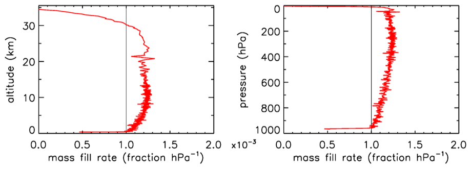
In Fig. 2 the outside air temperature first cools while in the troposphere, then becomes nearly constant in the tropopause and starts increasing again higher into the stratosphere. GMD008 was well insulated but still partially followed the outside temperatures with a delay. In the right panel the total amount of air in the tube is plotted relative to how much it would be if it had the same pressure and temperature everywhere in the tube as the outside air. The vertical line shows the ratio equaling 1 if they were the same. During ascent in the troposphere (up to about 10 km), the air in the tube is warmer and thus less dense than outside air. In the tropopause the tube continues to cool so that the “deficit” becomes smaller, but at higher altitudes, around ∼25 km, the amount by which the density in the tube is higher than outside becomes substantial relative to the low outside pressure – as a result the ratio at ∼34 km altitude becomes a bit larger than 1. Then, during descent the outside pressure increases rapidly, and the inflow cannot keep up because the viscosity of air at low pressure is the same as at 1 bar (see Sect. 3). Back in the troposphere the tube warms up but much more slowly than outside air. When the tube hits the ground, it is colder than the ambient air temperature so that the ratio is greater than 1.

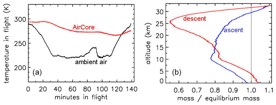
Figure 2 Flight of GMD008. (a) Temperatures in Kelvin. (b) How far the mass inside the tube is out of equilibrium with ambient air.

In Fig. 3 the fill rate is plotted (moles per hectopascal of ambient pressure gain) divided by the final fill (moles of air) at valve closure. At sea level the final pressure is close to 1013 hPa so that the average fraction of the final fill amount per hectopascal will be approximately 0.001. The uptick upon landing (very close to the x axis) is the result of a bit of air still entering the tube initially while ambient pressure stops changing, neglecting high-frequency noise. If the valve is not closed quickly, this will reverse because as the tube warms up on the ground, the last air that came in will be expelled. At high altitudes it takes time for the fill to start because ambient pressure needs to build up enough to force the air in. The highest altitude was 32.4 km, at 7.7 hPa ambient pressure. The fill starts at 31.6 km and a pressure of 8.5 hPa, slowly at first and gradually becoming faster. To compare the start of the fill between AirCore designs with different diameters and valves, we could take the point at which the fill rate is $\mathrm{0.5}\times {\mathrm{10}}^{-\mathrm{3}}$. In this case the “half-fill-rate point” is at 27.3 km and an ambient pressure of 17.3 hPa. We will see below that the fill starts much faster with larger diameters. Figure 4 shows detail of flow and pressure inside the tube for the flight on 20 June 2019 at the start of the descent. Initially the inflow velocity is negative. It is outflow, zero at the closed end and increasing toward the open end. After 14 s into the descent (light-blue curve) the outflow has weakened considerably, and the pressure gradient near the open end is much smaller. Inflow starts after 19 s, very slowly at first, while at the same time the flow in most of the tube is still negative (outflow toward the open end), consistent with the pressure gradients.

Figure 3 Flight of GMD008. The vertical line at $\mathrm{1.0}\times {\mathrm{10}}^{-\mathrm{3}}$ is approximately the expected rate of sample inflow. The dashed line at $\mathrm{0.5}\times {\mathrm{10}}^{-\mathrm{3}}$ represents the half-fill-rate point (see main text).

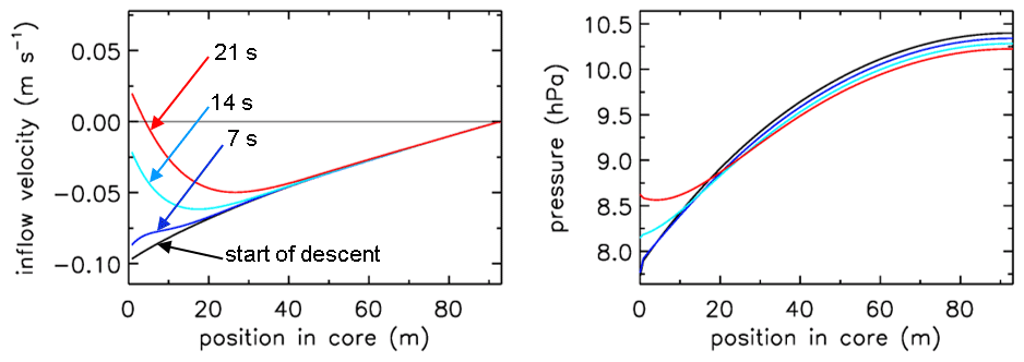
Figure 4 Flight of GMD008. The turnaround at high altitude. Inflow velocity and pressure inside the AirCore from the moment the ascent stops and descent begins. Times are in seconds after start descent.

Table 1 Comparison of start of fill process for two AirCore configurations.

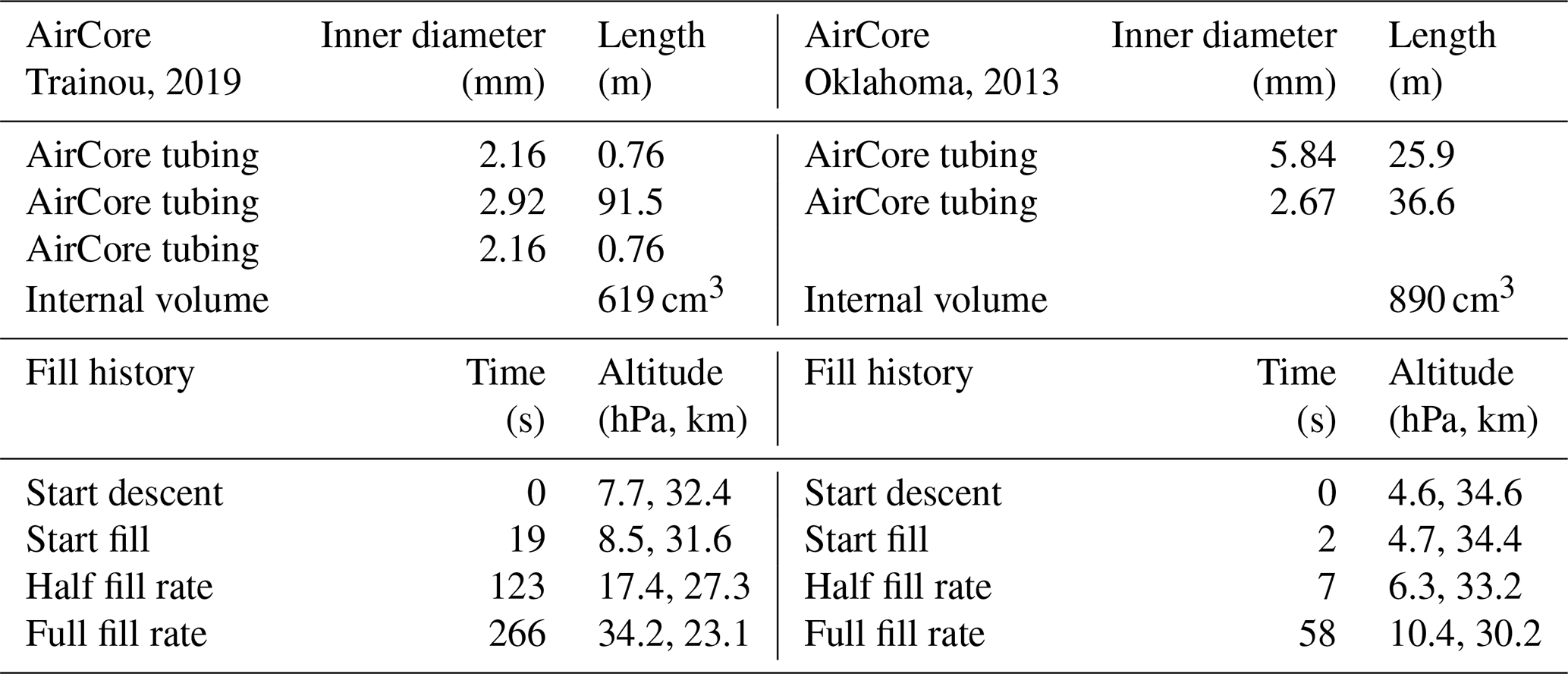
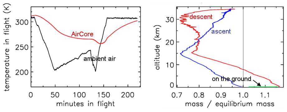
Let us look now at an AirCore with larger diameters (Fig. 5). This one had 26 m of $\mathrm{1}/\mathrm{4}$ in. (inner diameter of 5.84 mm) tubing at the open end and 37.6 m of $\mathrm{1}/\mathrm{8}$ in. (inner diameter of 2.67 mm) tubing at the closed end, with a total internal volume of 890 cm³. The high-altitude fill history of the two AirCores is summarized in Table 1. In front of the open end was a valve, the dryer (large magnesium perchlorate particles), and then another valve connecting to the AirCore tube. It was flown in Oklahoma, US (37.2^∘ N, 97.8^∘ W), on 23 July 2013. While the AirCore used near Trainou, France, experienced a temperature range of 15 K, the less well-insulated AC01 in Oklahoma saw a range of 57 K. At the moment of landing the average temperature of the tube was ∼40 K cooler than the ambient temperature. Figure 5 shows the flight data until the moment of valve closure. The valve remained open for 62 min after landing so that the lowest portion of the atmospheric sample, between pressure altitudes of 844 and 967 hPa (1565 to 352 m), was expelled as the AirCore warmed up. The descent started at 34.6 km altitude (4.6 hPa). The lowest relative mass deficit (∼27 %) was reached around 30 km, in contrast to the Trainou flight with 50 % at 27 km altitude respectively. The half-fill-rate point of $\mathrm{0.5}\times {\mathrm{10}}^{-\mathrm{3}}$ hPa⁻¹ is reached at 33.2 km altitude and 6.2 hPa of ambient pressure, a sampling altitude gain of almost 6 km compared to the Trainou flight. If the total amount of the initial fill air that remained in the tube can be carefully measured, it would give an independent estimate of the pressure altitude of the half-fill-rate point. The fill rate below ∼8 km falls off noticeably as the warming rate of the tube speeds up. The negative mass fill rate while on the ground cannot be portrayed in Fig. 6 because ambient pressure remains constant. This AirCore design contains a larger fraction of stratospheric air than GML008, mostly because of the wider diameter but also because it was allowed to cool more.

Figure 5 Flight of AC01 in Oklahoma.

Figure 6 Flight of AC01 in Oklahoma. Compare with Fig. 3.

If one wants to sample still higher into the stratosphere, the diameter of the first 10 to 20 m at the open end needs to be widened further than 6 mm diameter (Table 1). All of this is consistent with Fig. (7), where we also see that at the start of the descent the outflow velocity inside the tube drops by a factor of ∼4 when, moving from the back to the open end, at 25.9 m the tube diameter becomes wider by a factor of ∼2. This applies of course also to the inflow as shown by the red curve. At the same point the pressure gradient becomes less steep by the same factor of 4. The fill starts at an ambient pressure of 4.7 hPa. We also note that in this case the pressure drop inside the two valves and the dryer is a large part of the overall pressure drop across the entire tube, an effect that becomes more pronounced as the tube diameter gets larger.

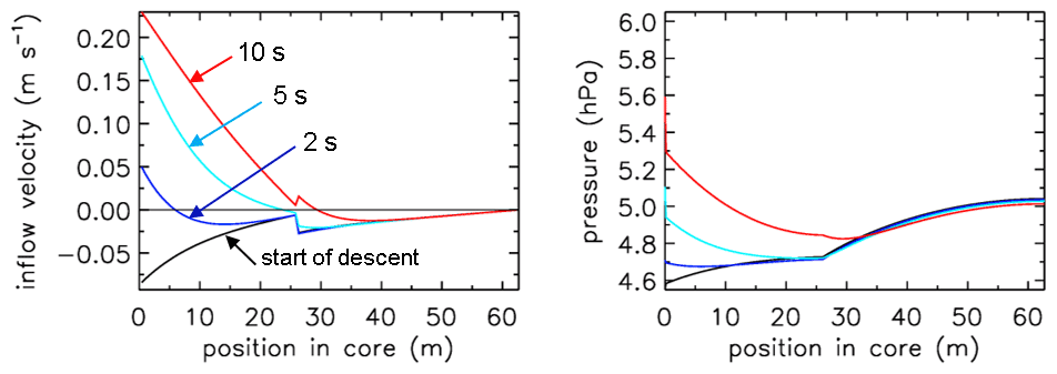
Figure 7 Flight of AC01 in Oklahoma, showing inflow velocity and pressure gradients. Compare with Fig. 4. Note the much smaller fill delay than in Fig. 4. The pressure drop across the two valves and dryer is visible here along the y axis (pressure).

In these calculations I have experimented with another strategy to fill the AirCore. One could launch it with both valves open, but the one in the back is closed as soon as the descent starts. That would decrease the amount of fill air that remains in the back. However, the difference from having the back valve closed during the entire flight is negligible.

5 Valves

So far the treatment of valves and the dryer has been missing from this description. As a first approximation we could treat the valves as short pieces of tubing with a reasonably “average” inner diameter and length such that their internal volume is correct. This does not provide enough flow resistance when we compare it to differential-pressure measurements made during flights between the closed end of the AirCore and the outside ambient air (Fig. 8).

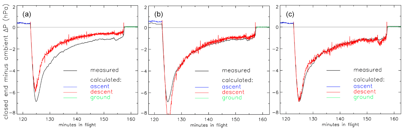
Figure 8 Pressure difference (ΔP) between the closed end of the tube and outside air during the descent portion of the flight of AC01 in Oklahoma as a function of elapsed time in flight. Black: measured pressure difference (hPa). Red: calculated ΔP with three different treatments of the valves. (a) Fixed inner diameter and length. (b) Same as in (a) but optimized. (c) Using optimized C_v and X_TPR (see main text) values.

In panel (a) we calculate that during the descent the air enters the tube too easily so that the altitudes assigned to the air sample in the stratosphere would be biased high. We could decrease the chosen average inner diameter (not a well-defined value) of the valves (panel b), optimized so that the difference between calculated and measured ΔP during the entire descent, from minute 123 to 157, is minimized. However, it is clear that this effective or apparent inner diameter needs to change during the flight. Using C_v values and a description of choked flow is clearly better. In panel (c) we have chosen the C_v and X_TPR (see below) values such that the average difference from minute 123 to 157 is zero and the standard deviation of differences is minimized. This implicitly includes any effects caused by the dryer in between the two valves.

The flow inside a valve can be complicated, with sharp corners, turbulence, sudden acceleration through a flow restriction with its associated heating and cooling of the gas, etc. The industry has introduced flow coefficients (C_v in the US and K_v elsewhere) as an empirical approach to flow calculations, as in the Swagelok (2020) brochure. The expressions for air, slightly generalized from Swagelok, for gas flow are as follows. For low-pressure drop flow, we have

$$\begin{array}{}\text{(5a)}& Q_n=\mathrm{6950}{C}_{\mathrm{v}}{P}_{\mathrm{1}}\left(\mathrm{1}-{\displaystyle \frac{X}{\mathrm{3}{X}_{\mathrm{TPR}}}}\right)\sqrt{{\displaystyle \frac{X}{T_{\mathrm{1}}}}},\end{array}$$

where Q_n is in liters per minute at standard conditions of 1 bar and 0 ^∘C; P₁ and T₁ are pressure (bar) and temperature (Kelvin) upstream of the valve; ΔP is the pressure drop across the valve; X is the pressure drop ratio, $\mathrm{\Delta }P/P_{\mathrm{1}}$; and X_TPR is the terminal pressure drop ratio between 0 and 1, above which we have choked flow. Under choked flow conditions the flow is fully independent of P and T downstream of the valve. It is also important to know that the flow coefficient C_v is not a pure number but has physical quantities and units embedded in it.

For a high-pressure drop (X>X_TPR), we have

$$\begin{array}{}\text{(5b)}& Q_n=\mathrm{6950}{C}_{\mathrm{v}}{P}_{\mathrm{1}}{\displaystyle \frac{\mathrm{2}}{\mathrm{3}}}\sqrt{{\displaystyle \frac{X_{\mathrm{TPR}}}{T_{\mathrm{1}}}}},\end{array}$$

which is obtained from the previous expression by substituting X_TPR (a constant) for X. In these expressions we prefer to express the flow, instead of in standard liters per minute as in the Swagelok (2020) brochure, as 0.04403 mol min⁻¹. This is the same when using the molecular weight of dry air (28.97 g mol⁻¹), as a mass flow of 1.276 g min⁻¹.

In Fig. 8c we optimized both C_v and X_TPR to get the best match for the calculated pressure difference across the AirCore with the observed history during the descent. The value of X_TPR depends on valve design and may not be the same when flow goes in the opposite direction. Many valves have an arrow for flow direction printed on them. For many AirCore flights differential-pressure measurements have not been recorded. However, the valves (and also dryers) could be tested with a standard procedure (see Fig. 9 as one example). Alternatively or as a complementary check, a micro-spiking method during filling could be used (Wagenhäuser et al., 2021).

Figure 9 shows a potential test procedure for determining C_v and X_TPR values. The figure is drawn using the two expressions for Q_n above, for low flow and choked flow. Starting from a uniform pressure of 1 bar, the pressure at the downstream side is lowered in 10 hPa steps, at 2 s intervals. In this example C_v=0.01 and X_TPR=0.5 so that the transition to choked flow occurs at a pressure drop of 0.5 bar (panel a, upward arrow at 100 s). When the pressure at 10 m approaches zero, the flow speed is high, causing a significant pressure drop between 5 and 10 m.

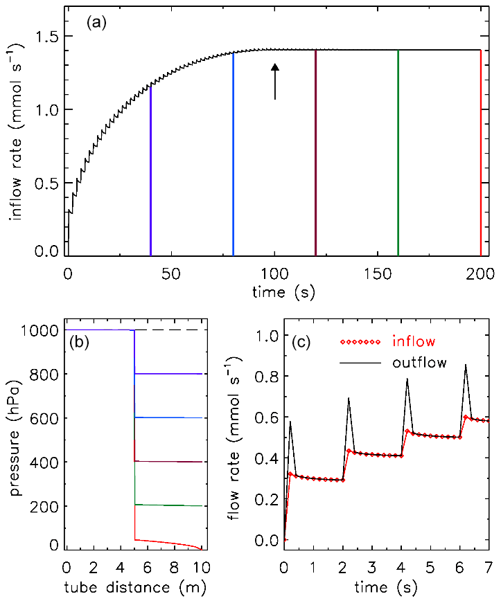
Figure 9 A potential test procedure to determine C_v and X_TPR values for valves. In this example there is 5 m of $\mathrm{1}/\mathrm{4}$ in. tubing (ID 5.84 mm) on each side. Outflow at the 10 m point (black curve) is shown in panels (a) and (c). There is a flow pulse at every step because the downstream 5 m section empties quickly. The time resolution is 0.2 s. Inflow at 0 m is shown as red diamond symbols in panel (c). (b) Pressure in the tube from time 0 (dashed line) at 40 s intervals, corresponding to the colors in panel (a).

6 Mixing inside the tube

The fill dynamics calculation has produced time series of air density, pressure and temperature, and flow velocity everywhere in the tube as a function of time, from the start of the fill process, which begins a varying amount of time after the AirCore has started its descent, to the time of valve closure. We divide the final amount of air in the tube at closure into 400–500 equal mass packets. Starting from 400 we increase the number, which shrinks the size of each packet, until the remaining fill air in the back of the tube comprises an exact integer number of packets. For each mass packet, after it has entered the tube, we follow it through the tube, as it is pushed toward the back while being compressed by packets entering later. The time steps are defined by when a new packet has fully entered, and they are longer at the start of the fill. The molecular diffusivity D and the Taylor diffusivity D_T are different at each step. However, the amount of spreading of a packet calculated at each time step k is decreased as the increasing pressure compresses the packet further. So the contribution of each step to the final spreading at valve closure is calculated by dividing the density during that time step by the final density in the tube. We are thus accumulating the 2Dt term of X_rms=(2Dt)^0.5, with Taylor diffusion added:

$$\begin{array}{}\text{(6)}& X_{\mathrm{rms}}=\sqrt{\mathrm{2}{\sum }_k\left(D_k+D_{T,k}\right){\displaystyle \frac{{\mathit{\rho }}_k}{{\mathit{\rho }}_{\mathrm{final}}}}{t}_k}.\end{array}$$

For an AirCore with (an almost) uniform diameter, we get mixing as in Fig. 10a. Close to the open end at position 0 m, there is very little mixing because the time to mix was short. Near the closed end at 93 m the spread of mixing deviates from what is seen in the first approximately $\mathrm{2}/\mathrm{3}$ of the tube because the fill started slowly, giving extra mixing time for the high-altitude samples that were later pushed to the back.

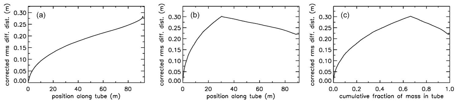
Figure 10 Root-mean-square diffusive mixing when the valve at position 0 is closed. (a) Flight of GMD008 in Trainou. (b) The same flight data but used to calculate the filling of a different AirCore, with 30.9 m of $\mathrm{1}/\mathrm{4}$ in. tubing at the open end and 60.1 m of $\mathrm{1}/\mathrm{8}$ in. at the closed end. (c) Same as (b) but plotted as the cumulative fraction of total mass, from 0 to 1.

For an AirCore with two sections of different diameters, we see an interesting effect (Fig. 10b). The air that comes in at high altitudes and ends up in the back of the tube has to go through the $\mathrm{1}/\mathrm{4}$ in. section first. When a packet enters the $\mathrm{1}/\mathrm{8}$ in. section, its spread becomes approximately 4 times larger, while its 2Dt accumulation term stays the same. Approximately, this is because the inner diameter (ID) matters, while the outer (OD) does not. To correct for the jump, we add another factor to Eq. (6), and we will call this corrected rms diffusion distance:

$$\begin{array}{}\text{(7)}& X_{\mathrm{rms}}=\sqrt{\mathrm{2}{\sum }_{\mathrm{k}}\left(D_k+D_{T,k}\right){\displaystyle \frac{{\mathit{\rho }}_k}{{\mathit{\rho }}_{\mathrm{final}}}}{\displaystyle \frac{(\text{dvol}/\mathrm{d}x{)}_k}{(\text{dvol}/\mathrm{d}x{)}_{\mathrm{ref}}}}{t}_k}.\end{array}$$

In Eq. (7) $\text{dvol}/\mathrm{d}x$ is the increment in volume per increment in the length of the tube, while ($\text{dvol}/\mathrm{d}x{)}_{\mathrm{ref}}$ is the total volume divided by the total length (both in units of m²). This prevents a jump at the 30 m position, but more importantly, what matters for mixing is the spread relative to total mass in the tube, not whether it is in the $\mathrm{1}/\mathrm{4}$ or $\mathrm{1}/\mathrm{8}$ in. section. From now on we call this configuration “$\mathrm{1}/\mathrm{4}$–$\mathrm{1}/\mathrm{8}$”. Figure 10b shows that air closer to the back has been in the $\mathrm{1}/\mathrm{4}$ in. section for a shorter time and thus experienced less mixing relative to mass. When plotting mixing not as a function of position but as a function of cumulative mass in the tube, Fig. 10c also shows that the $\mathrm{1}/\mathrm{8}$ in. section contains approximately $\mathrm{1}/\mathrm{3}$ of the total air sample.

Figure 11 Two additional cases of mixing upon valve closure. (a) Same AirCore $\mathrm{1}/\mathrm{4}$–$\mathrm{1}/\mathrm{8}$, but the flight data have been changed. (b) Same flight data as in Fig. 10a, but the AirCore configuration is $\mathrm{1}/\mathrm{4}$–$\mathrm{1}/\mathrm{8}$–$\mathrm{1}/\mathrm{4}$.

In Fig. 11a when the tube had descended to 850 mbar, the atmospheric pressure data were changed to simulate an updraft (lowering outside pressure) followed by a downdraft. The most recent seven mass packets were lost from the tube during the updraft and replaced by new air during the downdraft (above-average rate of increase of outside pressure). As a result, the air sample that just escaped from being lost is now adjacent to the replacement air, creating the jump in rms mixing because it has been ∼15 s longer in the tube than the first replacement air entering. In Fig. 11b the AirCore has now three sections, from the open to the closed end, first 30.1 m of $\mathrm{1}/\mathrm{4}$ in., then 52.1 m of $\mathrm{1}/\mathrm{8}$ in., and finally 10.1 m of $\mathrm{1}/\mathrm{4}$ in. diameter, which we will call “$\mathrm{1}/\mathrm{4}$–$\mathrm{1}/\mathrm{8}$–$\mathrm{1}/\mathrm{4}$”. This was done solely to illustrate clearly the effects of using different diameters. Similar to what we saw in Fig. 10a, the spread of mixing steepens near the closed end. Also those samples resided not long enough in the $\mathrm{1}/\mathrm{8}$ in. section to have much benefit in terms of slowing down the mixing, but between 0.80 and 0.85 they had been long enough in the $\mathrm{1}/\mathrm{8}$ in. section to have experienced less mixing than air ending up at the 0.57 point, the first transition between $\mathrm{1}/\mathrm{4}$ and $\mathrm{1}/\mathrm{8}$ in.

We will now express the amount of spreading (in both directions – twice the rms distance) of each equal-mass “packet” of air as a fraction of the total mass of air in the tube, assuming that the temperature inside the tube has become uniform. If that fraction were 0.01 everywhere in the tube, there would be slightly less than 100 independent samples in the AirCore. It would be slightly less because the remaining fill air in the back takes up space. Figure 12 shows a more realistic situation. Each sample takes up the same volume, separated by the blue vertical lines, producing vertical boxes. If there is almost no mixing, as in the case of the last sample that entered the AirCore, the sample almost completely fills the first volume (or box in Fig. 12a), which is indicated by the value of 1.0 on the y axis. The red curve centered on the second box has started to “leak” some sample into the adjoining boxes. The next samples shown are the 7th, 12th and 17th. For the latter, the sample is just starting to leak into boxes 15 and 19. To plot the start of this process correctly, each packet is subdivided into 13 equal portions. Narrow Gaussian spreading, slowly increasing further into the tube, is calculated for each portion and then summed. The width of each Gaussian is shown in Fig. 10c as a function of the fraction of cumulative mass in the tube, and the area of each curve is $\mathrm{1}/\mathrm{13}$ of the area of the box. This produces a constant value of 1.0 in the center, and only the outer portions reach into the neighboring boxes.

Figure 12 (a) Mixing of individual air packets (red) near the open end with their neighbors at valve closure for the case shown in Fig. 10c. (b) Mixing near the closed end (red), with vertical red lines centered on 0.97 showing the ±1σ points; the black curve being remaining fill air; and the sum of all actual sample packets, also of those not shown, being the red dashed line.

In Fig. 12b we plot the situation near the closed end. As in Fig. 12a, the mixing of only every fifth air packet is plotted, here ending with the first that came in at the highest altitude, centered approximately at 0.991. The remaining fill air in this case has the mass of four packets, and the curves of fill air and of the total air sample (sum of all packets) cross over at exactly the point where the fourth box from the right starts.

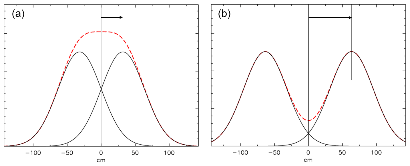
Figure 13 Mixing at a closed end. The AirCore is to the right of the 0 cm point. (a) The distribution of mixing started 1 h ago from a plane at 31.8 cm (1 root mean square of the distribution), indicated by the arrow. A fictitious “mirror” distribution is centered at −31.8 cm. The red dashed curve is the sum of the two distributions. (b) Same calculation, but the center of the distribution is twice as far from the end as in (a).

How we calculate mixing at a closed end (at x=0) is shown in Fig. 13. Diffusive mixing that would be to the left of x=0 is reflected toward positive values of x. The slope of the distribution must be zero at x=0 because any non-zero slope would imply a diffusive flux out of or into the tube. This is conveniently modeled by assuming a fictitious distribution mirrored relative to x=0, then the two are added, and the portion of the sum for positive values of x represents the mixing distribution near a closed end.

Let us assume that after the valve has been closed there has been a delay of 0.5 h before analysis starts. Therefore, additional diffusion has taken place, as shown in Fig. 14 for the case $\mathrm{1}/\mathrm{4}$–$\mathrm{1}/\mathrm{8}$–$\mathrm{1}/\mathrm{4}$ (Fig. 11b). The 2Dt term has been increased by an amount dependent on the diameter of the tube, normalized as in Eq. 7. In the upper right (panel b) the square root of the sum has been taken and then transformed into the spreading width relative to total mass in the tube. The width is defined here as the distance between the ±1σ points of the Gaussian, which contains ∼68 % of the probability distribution, shown in Fig. 14c at x=0.0410 and 0.0478 around the center at x=0.0444 and in Fig. 14d at x=0.9422 and 0.9518 around the center at x=0.9470. These numbers correspond to the full widths shown in Fig. 14b. The last packet to enter the tube is centered at x=0.0011 and 1σ=0.0033. Most of the diffusive spreading is to the right so that the peak is almost twice as high and the full width is a little over half as wide as the one centered on x=0.023.

Figure 14 Mixing after 30 min of storage, for AirCore $\mathrm{1}/\mathrm{4}$–$\mathrm{1}/\mathrm{8}$–$\mathrm{1}/\mathrm{4}$. (a) Sum (black) of the 2Dt accumulation during the flight (red) and during storage (blue; in units of m²). (b) Spreading width expressed as a fraction of the total mass in the tube. (c) Amount of spreading near what was the open end; for clarity only every 10th packet is shown. (d) Same, near the closed end. Vertical red lines show the ±1σ distances from the peak.

Often the AirCore is analyzed significantly later than 30 min after valve closure, and the measurement process itself may take 0.5 h. In Fig. 15 the state of mixing 4 h after valve closure has been calculated, and two AirCore configurations are compared. The spreading width of air packets near the closed end is nearly twice as large for the $\mathrm{1}/\mathrm{4}$–$\mathrm{1}/\mathrm{8}$–$\mathrm{1}/\mathrm{4}$ case as for the $\mathrm{1}/\mathrm{4}$–$\mathrm{1}/\mathrm{8}$ case, and the initial fill air penetrates almost 50 % further into the tube. It would in most cases not be a good idea to have a wide bore section at the closed end. If one waits 24 h (6 times longer) before starting the analysis, the spreading width near the closed end, centered at x=0.9470, is 2.32 times larger than after 4 h, not quite $\sqrt{\mathrm{6}}$ because after 4 h the spreading that occurred during the descent still makes a small but still noticeable contribution.

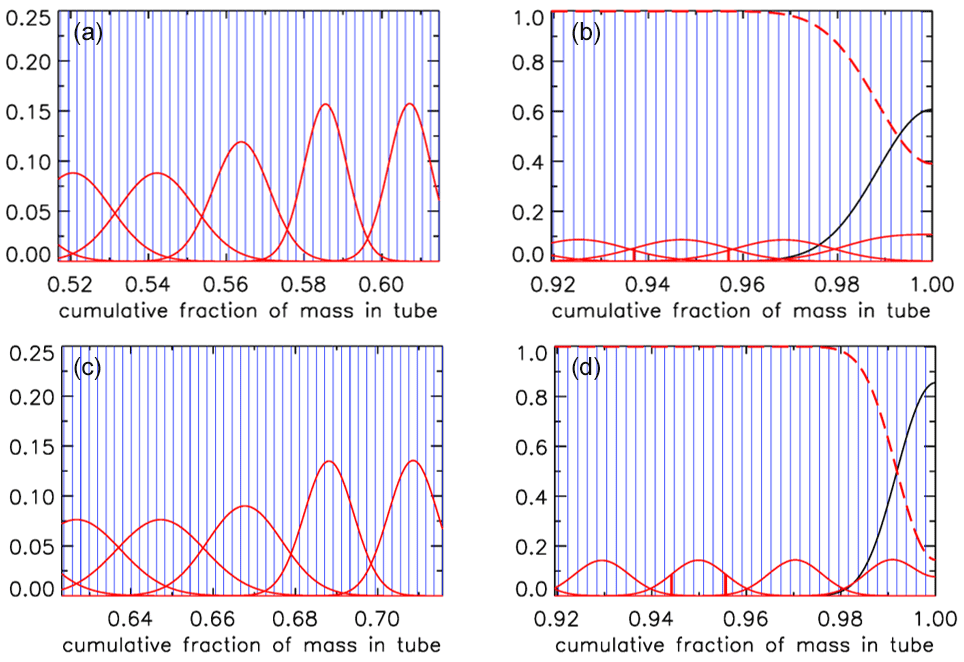
Figure 15 Mixing after 4 h of storage. (a) At the transition in diameter from $\mathrm{1}/\mathrm{4}$ to $\mathrm{1}/\mathrm{8}$ in., for AirCore $\mathrm{1}/\mathrm{4}$–$\mathrm{1}/\mathrm{8}$–$\mathrm{1}/\mathrm{4}$. (b) Near closed end, for $\mathrm{1}/\mathrm{4}$–$\mathrm{1}/\mathrm{8}$–$\mathrm{1}/\mathrm{4}$. (c) At the transition in diameter from $\mathrm{1}/\mathrm{4}$ to $\mathrm{1}/\mathrm{8}$ in., for AirCore $\mathrm{1}/\mathrm{4}$–$\mathrm{1}/\mathrm{8}$. (d) Near closed end, for $\mathrm{1}/\mathrm{4}$–$\mathrm{1}/\mathrm{8}$.

7 Potential information content of the AirCore

The mixing calculated above allows for a realistic and precise estimate of the altitude resolution of the full air sample, both when the AirCore is analyzed in the field promptly after landing or hours or even days later. When the air is slowly pushed through an analyzer, we obtain a quasi-continuous curve for the mole fraction of the gases of interest as a function of fractional cumulative mass in the tube which is linked to flight data such as pressure altitude, geometric altitude, latitude, and longitude as calculated from the filling dynamics. We define the information content as the number of independent air samples that are inside the tube or the number of degrees of freedom (DoF). Longer wait times before analysis decrease DoF. For example, 0.5 h after landing DoF is potentially 154 for the Trainou flight, while after another delay of 4 h, DoF has dropped to 67. This is “potential DoF” because it could be decreased further by additional mixing in the measurement cell or by successive analyzer cells measuring different gas species. In the section above we chose more than 400 equal-mass packets to calculate mixing. This was done to prevent a possibly low numerical resolution of the mixing calculation which would unnecessarily create a low bias in DoF estimates. Ideally, the measurement process could be modeled in a way similar to the fill and mixing calculation above, convolving the packets leaving the AirCore with a pulse response of the measurement cell. The response could be measured separately by introducing a sharp spike just before the cell and recording how it is mixed and flushed out. This would be similar to the spiking method described by Wagenhäuser et al. (2021). In the worst case the measurement cell would be perfectly mixed, giving rise to exponential flushing. In that case, after one cell volume has entered from the AirCore into the measurement cell, the latter still contains a fraction $\mathrm{1}/e$ of what went through the cell before so that the new volume comprises $(\mathrm{1}-\mathrm{1}/e)=\mathrm{0.63}$ of the cell loading. On the other hand, “plug flow” (like in the AirCore itself) would produce very little additional mixing, but there could still be some turbulent eddies near the entrance and exit of the cell. The actual influence of the measurement cell on mixing lies somewhere in between those two extremes.

8 Numerical implementation

The AirCore can consist of one or more sections of different lengths, each with a different inner diameter. For example, GML has flown AirCores with a wider bore at the open end and a narrow bore at the closed end, in order to get a better vertical resolution for the stratosphere. The sections can be divided into a number of smaller segments when Eq. (2) is discretized for a numerical solution (Fig. 16):

$$Q=-\mathit{\rho }{\displaystyle \frac{\mathit{\pi }{r}^{\mathrm{4}}}{\mathrm{8}\mathit{\eta }}}{\displaystyle \frac{\mathrm{d}P}{\mathrm{d}z}}\Rightarrow Q_j=-{\displaystyle \frac{P_j+P_{j+\mathrm{1}}}{R\left(T_j+T_{j+\mathrm{1}}\right)}}{\displaystyle \frac{\mathit{\pi }{r}_j^{\mathrm{4}}}{\mathrm{8}{\mathit{\eta }}_j}}{\displaystyle \frac{P_{j+\mathrm{1}}-P_j}{\mathrm{d}{z}_j}}.$$

Q_j is centered in the middle of segment dz_j. The first factor in Q_j is the average amount density (ρ_j). The pressure change at the boundary between segments dz_j−1 and dz_j caused by the imbalance of the flows Q_j−1 and Q_j is equal to that imbalance divided by the volume between the midpoints of dz_j−1 and dz_j. Adding in the pressure change due to temperature (Eq. 2), we get for the change at boundary j:

$$\begin{array}{}\text{(8)}& \begin{array}{rl}{\displaystyle \frac{\mathrm{d}{P}_j}{\mathrm{d}t}}={\displaystyle \frac{P_j}{T_j}}{\displaystyle \frac{\mathrm{d}{T}_j}{\mathrm{d}t}}& +{\displaystyle \frac{T_j}{\mathrm{0.5}\left(\mathrm{d}{z}_{j-\mathrm{1}}{r}_{j-\mathrm{1}}^{\mathrm{2}}+\mathrm{d}{z}_j{r}_j^{\mathrm{2}}\right)}}\\ & {\displaystyle \frac{P_j+P_{j+\mathrm{1}}}{T_j+T_{j+\mathrm{1}}}}{\displaystyle \frac{r_j^{\mathrm{4}}}{\mathrm{8}{\mathit{\eta }}_j}}{\displaystyle \frac{P_{j+\mathrm{1}}-P_j}{\mathrm{d}{z}_j}}\\ & -{\displaystyle \frac{T_j}{\mathrm{0.5}\left(\mathrm{d}{z}_{j-\mathrm{1}}{r}_{j-\mathrm{1}}^{\mathrm{2}}+\mathrm{d}{z}_j{r}_j^{\mathrm{2}}\right)}}\\ & {\displaystyle \frac{P_{j-\mathrm{1}}+P_j}{T_{j-\mathrm{1}}+T_j}}{\displaystyle \frac{r_{j-\mathrm{1}}^{\mathrm{4}}}{\mathrm{8}{\mathit{\eta }}_{j-\mathrm{1}}}}{\displaystyle \frac{P_j-P_{j-\mathrm{1}}}{\mathrm{d}{z}_{j-\mathrm{1}}}}.\end{array}\end{array}$$

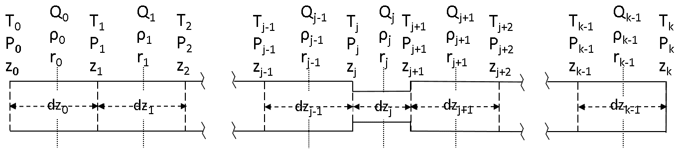
Figure 16 Coordinate system in the AirCore. The coordinate along the length of the tube is z. There are k segments, starting from the open end at z₀ to the closed end at z_k, between the vertical dashed lines. Amount flow (Q_n, mol s⁻¹) and amount density ρ_n (mol m⁻³), simply written as Q and ρ from here on out, are defined in the middle of each segment, with pressure (P) and temperature (T) being defined at the borders of each segment. The length (dz) as well as radius (r) of the segments may differ.

The first term $(P/T)(\mathrm{d}T/\mathrm{d}t)$ is handled separately from the two other terms describing the amount change. We write the latter two with the time step going from n to n+1 (superscript):

$$\begin{array}{}\text{(9)}& \begin{array}{rl}{P}_j^{n+\mathrm{1}}-P_j^n=[& {\displaystyle \frac{\mathrm{2}{T}_j^n\left(P_{j+\mathrm{1}}^n+P_j^n\right)}{T_{j+\mathrm{1}}^n+T_j^n}}{\displaystyle \frac{r_j^{\mathrm{4}}}{{\mathit{\eta }}_j}}{\displaystyle \frac{P_{j+\mathrm{1}}^{n+\mathrm{1}}-P_j^{n+\mathrm{1}}}{\mathrm{d}{z}_j}}\\ & -{\displaystyle \frac{\mathrm{2}{T}_j^n\left(P_{j-\mathrm{1}}^n+P_j^n\right)}{T_{j-\mathrm{1}}^n+T_j^n}}{\displaystyle \frac{r_{j-\mathrm{1}}^{\mathrm{4}}}{{\mathit{\eta }}_{j-\mathrm{1}}}}{\displaystyle \frac{P_j^{n+\mathrm{1}}-P_{j-\mathrm{1}}^{n+\mathrm{1}}}{\mathrm{d}{z}_{j-\mathrm{1}}}}]\\ & {\displaystyle \frac{t^{n+\mathrm{1}}-t^n}{\mathrm{8}\left(\mathrm{d}{z}_{j-\mathrm{1}}{r}_{j-\mathrm{1}}^{\mathrm{2}}+\mathrm{d}{z}_j{r}_j^{\mathrm{2}}\right)}}.\end{array}\end{array}$$

On the right hand side we have defined the pressure differences at the end of the time step. The reason is to make the solution of the matrix equation described below unconditionally stable. This method has been described as “fully implicit” or “backward time” (Press et al., 1986). We leave the pressure and temperature averages as defined at the start of the time step. They determine the average amount density of the air and do not create any numerical instability. Equation (9) can be further re-arranged, for j=1 to k−1, as

$$\begin{array}{}\text{(10)}& \begin{array}{rl}{P}_j^n=& -{\displaystyle \frac{t^{n+\mathrm{1}}-t^n}{\mathrm{8}\left(\mathrm{d}{z}_{j-\mathrm{1}}{r}_{j-\mathrm{1}}^{\mathrm{2}}+\mathrm{d}{z}_j{r}_j^{\mathrm{2}}\right)}}\\ & \left[{\displaystyle \frac{\mathrm{2}{T}_j^n\left(P_{j+\mathrm{1}}^n+P_j^n\right)}{T_{j+\mathrm{1}}^n+T_j^n}}{\displaystyle \frac{r_j^{\mathrm{4}}}{{\mathit{\eta }}_j\mathrm{d}{z}_j}}\right]P_{j+\mathrm{1}}^{n+\mathrm{1}}\\ & +\left(\mathrm{1}+{\displaystyle \frac{t^{n+\mathrm{1}}-t^n}{\mathrm{8}\left(\mathrm{d}{z}_{j-\mathrm{1}}{r}_{j-\mathrm{1}}^{\mathrm{2}}+\mathrm{d}{z}_j{r}_j^{\mathrm{2}}\right)}}\right)\\ & [{\displaystyle \frac{\mathrm{2}{T}_j^n\left(P_{j+\mathrm{1}}^n+P_j^n\right)}{T_{j+\mathrm{1}}^n+T_j^n}}{\displaystyle \frac{r_j^{\mathrm{4}}}{{\mathit{\eta }}_j\mathrm{d}{z}_j}}+{\displaystyle \frac{\mathrm{2}{T}_j^n\left(P_{j-\mathrm{1}}^n+P_j^n\right)}{T_{j-\mathrm{1}}^n+T_j^n}}\\ & {\displaystyle \frac{r_{j-\mathrm{1}}^{\mathrm{4}}}{{\mathit{\eta }}_{j-\mathrm{1}}\mathrm{d}{z}_{j-\mathrm{1}}}}]P_j^{n+\mathrm{1}}-{\displaystyle \frac{t^{n+\mathrm{1}}-t^n}{\mathrm{8}\left(\mathrm{d}{z}_{j-\mathrm{1}}{r}_{j-\mathrm{1}}^{\mathrm{2}}+\mathrm{d}{z}_j{r}_j^{\mathrm{2}}\right)}}\\ & \left[{\displaystyle \frac{\mathrm{2}{T}_j^n\left(P_{j-\mathrm{1}}^n+P_j^n\right)}{T_{j-\mathrm{1}}^n+T_j^n}}{\displaystyle \frac{r_{j-\mathrm{1}}^{\mathrm{4}}}{{\mathit{\eta }}_{j-\mathrm{1}}\mathrm{d}{z}_{j-\mathrm{1}}}}\right]P_{j-\mathrm{1}}^{n+\mathrm{1}}.\end{array}\end{array}$$

This is a tridiagonal matrix equation, $\mathbf{A}\mathrm{•}{\mathit{P}}^{n+\mathrm{1}}={\mathit{P}}^n$, linking the k+1 dimensional pressure vector Pⁿ⁺¹ at the end of the time step to the pressure vector Pⁿ at the start of the time step. The solution is ${\mathit{P}}^{n+\mathrm{1}}={\mathbf{A}}^{-\mathrm{1}}\mathrm{•}{\mathit{P}}^n$, in which A⁻¹ is the inverse matrix calculated by the subroutine TRISOL which is the IDL version of TRIDAG described by Press et al. (1986). If the tube is closed at z=0, then in the first line of A the first (diagonal) and second (above the diagonal) element (all others are zero) are respectively

$$\mathrm{1}+{\displaystyle \frac{t^{n+\mathrm{1}}-t^n}{\mathrm{8}\left(\mathrm{d}{z}_{\mathrm{0}}{r}_{\mathrm{0}}^{\mathrm{2}}\right)}}{\displaystyle \frac{\mathrm{2}{T}_{\mathrm{1}}^n\left(P_{\mathrm{1}}^n+P_{\mathrm{0}}^n\right)}{T_{\mathrm{1}}^n+T_{\mathrm{0}}^n}}{\displaystyle \frac{r_{\mathrm{0}}^{\mathrm{4}}}{{\mathit{\eta }}_{\mathrm{0}}\mathrm{d}{z}_{\mathrm{0}}}}$$

and

$$-{\displaystyle \frac{t^{n+\mathrm{1}}-t^n}{\mathrm{8}\left(\mathrm{d}{z}_{\mathrm{0}}{r}_{\mathrm{0}}^{\mathrm{2}}\right)}}{\displaystyle \frac{\mathrm{2}{T}_{\mathrm{1}}^n\left(P_{\mathrm{1}}^n+P_{\mathrm{0}}^n\right)}{T_{\mathrm{1}}^n+T_{\mathrm{0}}^n}}{\displaystyle \frac{r_{\mathrm{0}}^{\mathrm{4}}}{{\mathit{\eta }}_{\mathrm{0}}\mathrm{d}{z}_{\mathrm{0}}}}.$$

If the tube is open at z=0, then the first element of the first line equals 1 and all others are 0. In this case P₀ is defined at all times by the outside atmospheric pressure or by a defined pressure from a cylinder. There is no influence from any place inside the tube. The algorithm also allows the other end to be either closed or open to outside air. If closed, then the last two elements of the (k+1)^st row are respectively

$$-{\displaystyle \frac{t^{n+\mathrm{1}}-t^n}{\mathrm{8}\left(\mathrm{d}{z}_{k-\mathrm{1}}{r}_{k-\mathrm{1}}^{\mathrm{2}}\right)}}{\displaystyle \frac{\mathrm{2}{T}_{k-\mathrm{1}}^n\left(P_{k-\mathrm{1}}^n+P_k^n\right)}{T_{k-\mathrm{1}}^n+T_k^n}}{\displaystyle \frac{r_{k-\mathrm{1}}^{\mathrm{4}}}{{\mathit{\eta }}_{k-\mathrm{1}}\mathrm{d}{z}_{k-\mathrm{1}}}}$$

and

$$\mathrm{1}+{\displaystyle \frac{t^{n+\mathrm{1}}-t^n}{\mathrm{8}\left(\mathrm{d}{z}_{k-\mathrm{1}}{r}_{k-\mathrm{1}}^{\mathrm{2}}\right)}}{\displaystyle \frac{\mathrm{2}{T}_{k-\mathrm{1}}^n\left(P_{k-\mathrm{1}}^n+P_k^n\right)}{T_{k-\mathrm{1}}^n+T_k^n}}{\displaystyle \frac{r_{k-\mathrm{1}}^{\mathrm{4}}}{{\mathit{\eta }}_{k-\mathrm{1}}\mathrm{d}{z}_{k-\mathrm{1}}}}.$$

If both sides are open, each with a different defined constant pressure, then after initially transient, the flow settles to steady-state flow corresponding to Poiseuille's equation.

This describes the core algorithm, of which there are two versions, called tubeflowstep3.pro and tubeflowstep3Cv.pro. They have been programmed in Interactive Data Language (IDL). These algorithms have the flexibility to accommodate segments of the tube that have different lengths as well as diameters, flows in both directions, one or two valves open, a temperature gradient along the tube with its corresponding viscosity gradient, and variable time steps.

Another routine, called analyzefill_Gaus_ict.pro, reads the lengths and diameters of tube sections; valves and dryer; and the relevant flight data, namely outside air pressure and temperature and the temperature of the AirCore at different locations along the tube, all as a function of time. If C_v and X_TPR values of valves are defined, they will be used. In that case tubeflowstep3Cv.pro nudges the apparent inner diameter of one or more valves for a given flow toward satisfying Eq. (5) (see Sect. 5). This needs to be iterated because when we change the internal valve diameter the pressures and flows will then adjust elsewhere in the tube.

The analyzefill_Gaus_ict.pro program also reads altitude, latitude, and longitude, but they are not needed for the flow dynamics calculation per se; analyzefill_Gaus_ict.pro also sets up the coordinate system and initializes variables. By calling tubeflowstep3.pro at every time step or tubeflowstep3Cv.pro if C_v and X_TPR values are defined, it calculates the pressure in the tube, the amount of air and the amount flow, and the flow velocity, all as a function of time and location in the tube. This is how altitude, pressure altitude, latitude, and longitude are tied to position in the tube. The _Gauss portion of the name indicates that Gaussian mixing is used as described in this paper, and _ict indicates that the program expects the needed information about the tube and the flight in the ICARTT (International Consortium for Atmospheric Research on Transport and Transformation) file format, which is the format currently used by the GML AirCore project.

Although developed simultaneously with analyzefill_Gaus_ict.pro for the passively filled AirCore, the tubeflowstep3Cv program can also be used to model flow when the AirCore is actively filled with a pump and some form of flow and pressure control. In that case a program equivalent to analyzefill_Gaus_ict.pro would need to be developed.

Importantly, the code in analyzefill_Gaus_ict.pro also produces diagnostic graphics showing how the fill proceeded. In fact, all figures in this paper have been produced by analyzefill_Gaus_ict.pro except for Figs. 9 and 13.

9 Some recommendations for improvements in the analysis of AirCores

Laboratory measurements of the flow properties of valves, as expressed in the flow coefficient C_v and the terminal pressure drop ratio X_TPR, as well as the flow properties of dryers (permeability is more important than porosity) could be helpful for further improving the dynamics code as described in this paper and will be especially helpful for potential revisions of sample altitude assignments of older flights.

The precision of the sample mixing estimates could be improved by laboratory measurements of the pulse response of analyzers, especially when an AirCore is analyzed quickly in the field because very little mixing has yet occurred for the air that came in last.

In addition to measuring the pressure inside the tube during a flight at the closed end, one could consider measuring the pressure inside at a place closely behind the valve(s) plus dryer at the open end. It does not need to be done routinely, but it would give a history of the total pressure drop across the valve and dryer only.

In cases where people want to fly AirCores without a dryer, it could be helpful to study wall effects. Water vapor tends to adhere tightly to many surfaces, and as anyone experienced with vacuums knows, it can take a long time to pry it off the walls. One possible experiment would be to inject a short pulse of wet air at one end of a dry tube and register what comes out at the other end. How much stays behind, and for how long? How does that affect other species? In general, wall effects could make the AirCore into a (very poor) gas chromatograph if gases have sufficiently different adsorption/desorption properties.