A relaxed eddy accumulation (REA) LOPAP system for flux measurements of nitrous acid (HONO)

In the present study a relaxed eddy accumulation (REA) system for the quantification of vertical fluxes of nitrous acid (HONO) was developed and tested. The system is based on a three-channel long-path absorption photometer (LOPAP) instrument, for which two channels are used for the updrafts and downdrafts, respectively, and a third one for the correction of chemical interferences. The instrument is coupled to a REA gas inlet, for which an ultrasonic anemometer controls two fast magnetic valves to probe the two channels of the LOPAP instrument depending on the vertical wind direction. A software (PyREA) was developed, which controls the valves and measurement cycles, which regularly alternates between REA, zero and parallel ambient measurements. In addition, the assignment of the updrafts and downdrafts to the physical LOPAP channels is periodically alternated, to correct for differences in the interferences of the different air masses. During the study, only small differences of the interferences were identified for the updrafts and downdrafts excluding significant errors when using only one interference channel. In laboratory experiments, high precision of the two channels and the independence of the dilution-corrected HONO concentrations on the length of the valve switching periods were demonstrated.

A field campaign was performed in order to test the new REA-LOPAP system at the TROPOS monitoring station in Melpitz, Germany. HONO fluxes in the range of $-\mathrm{4}\times {\mathrm{10}}^{\mathrm{13}}$ molecules m⁻² s⁻¹ (deposition) to $+\mathrm{1.0}\times {\mathrm{10}}^{\mathrm{14}}$ molecules m⁻² s⁻¹ (emission) were obtained. A typical diurnal variation of the HONO fluxes was observed with low, partly negative fluxes during night-time and higher positive fluxes around noon. After an intensive rain period the positive HONO emissions during daytime were continuously increasing, which was explained by the drying of the uppermost ground surfaces. Similar to other campaigns, the highest correlation of the HONO flux was observed with the product of the NO₂ photolysis frequency and the NO₂ concentration (J(NO₂)⋅[NO₂]), which implies a HONO formation by photosensitized conversion of NO₂ on organic surfaces, such as humic acids. Other postulated HONO formation mechanisms are also discussed but are tentatively ranked being of minor importance for the present field campaign.

1 Introduction

During the last 25 years, high nitrous acid (HONO) mixing ratios have been observed during daytime under very different environmental conditions pointing to a major contribution of HONO photolysis to the oxidation capacity of the lower atmosphere (Neftel et al., 1996; Zhou et al., 2002a; Kleffmann et al., 2005; Acker et al., 2006; Elshorbany et al., 2009; Villena et al., 2011; Li et al., 2012; Yang et al., 2014; Hou et al., 2016; Lee et al., 2016; Tan et al., 2018; Slater et al., 2020). These high HONO levels can only be explained by strong daytime sources, for which (i) heterogeneous reduction of nitrogen dioxide (NO₂) in the presence of organic photosensitizers (George et al., 2005; Stemmler et al., 2006, 2007; Sosedova et al., 2011; Han et al., 2016a, b, 2017; Yang et al., 2021a), (ii) heterogeneous photolysis of nitric acid/nitrate (Zhou et al., 2003, 2011; Laufs and Kleffmann, 2016; Ye et al., 2016, 2017; Romer et al., 2018; Shi et al., 2021) and (iii) bacterial production of nitrite in soil (Su et al., 2011; Oswald et al., 2013; Maljanen et al., 2013; Oswald et al., 2015; Scharko et al., 2015; Weber et al., 2015) and/or desorption of adsorbed HONO from soil surfaces during daytime (Donaldson et al., 2014; VandenBoer et al., 2014, 2015) have been identified. In contrast, other proposed sources, like the gas-phase reaction of excited NO₂ with water (Crowley and Carl, 1997; Li et al., 2008; Carr et al., 2009; Amedro et al., 2011), the photolysis of nitro-phenols or similar compounds (Bejan et al., 2006; Yang et al., 2021b), and the gas-phase reaction of HO₂⋅H₂O complexes with NO₂ (Li et al., 2014, 2015; Ye et al., 2015), are of minor importance. Except for proposed HONO formation by particle nitrate photolysis (Ye et al., 2016, 2017), mainly ground surface sources have yet been identified in laboratory and field studies to explain atmospheric HONO formation during daytime in the atmosphere (Kleffmann, 2007). This is in good agreement with recent HONO gradient studies during daytime by the MAX-DOAS technique (Garcia-Nieto et al., 2018; Ryan et al., 2018; Xing et al., 2021).

In most field studies, the daytime HONO source strength was determined from HONO levels exceeding theoretical photostationary state (PSS) values, for which correlations of the daytime source with the photolysis rate coefficient J(NO₂) or the irradiance and the NO₂ concentration were often observed (Vogel et al., 2003; Su et al., 2008; Elshorbany et al., 2009; Sörgel et al., 2011; Villena et al., 2011; Wong et al., 2012; Lee et al., 2016; Crilley et al., 2016). In these studies, the HONO source is mathematically treated as a gas-phase process, despite its heterogeneous origin. Thus, the quantification of the daytime source is erroneous and depends on the height of the measurements above the ground and the vertical mixing of the atmosphere. In addition, the assumed PSS conditions may also not be fulfilled when HONO and its precursors are measured close to their sources (Lee et al., 2013; Crilley et al., 2016).

In contrast, flux measurements are able to give direct information about ground surface production and deposition and are a better tool to quantify ground sources of HONO in the lower atmosphere. Available flux observations indicate different HONO precursors. Harrison and Kitto (1994), Ren et al. (2011), and Laufs et al. (2017) found a relationship of the HONO flux with the NO₂ concentration and also its product with light intensity, which can be explained by the photosensitized conversion of NO₂ on humic acid surfaces (Stemmler et al., 2006). In contrast, for grassland spread with manure upward HONO fluxes could not be explain by an NO₂-driven mechanism (Twigg et al., 2011). For high nitrogen soil content, e.g. after fertilization, HONO fluxes up to 2 orders of magnitude higher compared to most other studies were recently observed in soil chambers (Xue et al., 2019; Tang et al., 2019). Thus, the latter three studies point to a soil-nitrogen-driven HONO formation mechanism. In contrast, Zhou et al. (2011) observed a correlation of the HONO flux with adsorbed nitric acid and short wavelength radiation, which was explained by photolysis of nitric acid adsorbed on canopy surfaces. Finally, for flux measurements in a forest clearing dominant formation processes explaining the positive daytime HONO fluxes remained unclear. In the same study at a co-located forest floor, only net HONO deposition was observed at the much lower irradiance levels compared to the forest clearing (Sörgel et al., 2015). The difference could be explained again by a photolytic HONO formation mechanism. In conclusion, based on available HONO flux studies, the origin of the main ground surface daytime HONO source is still controversially discussed.

Nowadays, eddy covariance (EC) is the most commonly applied method to measure fluxes between the surface and the atmosphere. The lack of HONO instruments, however, which are fast and sensitive enough for the EC method, requires the use of indirect methods like the aerodynamic gradient (AG) method (Harrison and Kitto, 1994; Twigg et al., 2011; Sörgel et al., 2015; Laufs et al., 2017) or the relaxed eddy accumulation (REA) method (Ren et al., 2011; Zhou et al., 2011; Zhang et al., 2012).

In the present study a relaxed eddy accumulation system for the quantification of vertical fluxes of HONO based on the long-path absorption photometer (LOPAP) technique was developed and tested in the laboratory and in the atmosphere.

2 The REA method

Turbulent transport is the most important process for the exchange of energy and trace gases between the ground and the atmosphere. When only slow instruments are available, the REA method is used to determine fluxes of trace gases, for which air masses are collected and analysed in two channels depending on the sign of the vertical wind (w) (Businger and Oncley, 1990). According to meteorological convention, positive and negative vertical wind directions reflect updrafts and downdrafts, respectively. Controlled by the vertical wind data measured by a 3D anemometer, fast valves are used to separate the different air masses to feed the two channels of the instrument. With a constant sample flow rate, the flux F_c of a trace gas c is calculated according to Eq. (1) from the mean concentration difference of the two channels $\left(\stackrel{\mathrm{‾}}{c_{\mathrm{up}}}-\stackrel{\mathrm{‾}}{c_{\mathrm{down}}}\right)$, the standard deviation of the vertical wind speed σ_w and a coefficient b₀, which is 0.627 under ideal joint Gaussian distribution of w and c (Wyngaard and Moeng, 1992; Ammann and Meixner, 2002; Sakabe et al., 2014):

$$\begin{array}{}\text{(1)}& F_c=b_{\mathrm{0}}\cdot {\mathit{\sigma }}_{\mathrm{w}}^{\mathrm{30}\min }\cdot \left(\stackrel{\mathrm{‾}}{c_{\mathrm{up}}}-\stackrel{\mathrm{‾}}{c_{\mathrm{down}}}\right).\end{array}$$

An averaging interval of typically 30 min is chosen to ensure that all eddies of different sizes and frequencies are captured, which contribute to the turbulent transport. Several field studies have shown that, depending on the stability of the atmosphere, the coefficient b₀ deviates from the ideal value and can be in the range of 0.51–0.62 (Baker et al., 1992; Katul et al., 1996; Ammann and Meixner, 2002).

To increase the measured concentration difference and to improve the signal-to-noise ratio, the use of a deadband is recommended (Businger and Oncley, 1990; Oncley et al., 1993). Here, sample air is collected only when the vertical wind speed is outside a defined deadband of the width ±w₀ around zero, while smaller eddies with low energy are not accounted for. Besides decreasing the flux errors, the use of a deadband also conserves the used valves by reducing the valve switching frequency. The half-width of the deadband w₀ is determined from the variance of the vertical wind ${\mathit{\sigma }}_{\mathrm{w}}^{\mathrm{5}\min }$ during the past 5 min:

$$\begin{array}{}\text{(2)}& w_{\mathrm{0}}=K\cdot {\mathit{\sigma }}_{\mathrm{w}}^{\mathrm{5}\min }.\end{array}$$

Depending on the turbulence distribution and the concentration of c, K values in the range 0.5–1 are used. Equation (1) can be reformulated when a deadband is used:

$$\begin{array}{}\text{(3)}& F_c=b\cdot {\mathit{\sigma }}_{\mathrm{w}}^{\mathrm{30}\min }\cdot \left(\stackrel{\mathrm{‾}}{c_{\mathrm{up}(w>w_{\mathrm{0}})}}-\stackrel{\mathrm{‾}}{c_{\mathrm{down}(w<-w_{\mathrm{0}})}}\right).\end{array}$$

Often variable b parameters are calculated for each averaging interval, for which different methods have been developed. By the proxy method, a passive scalar s (e.g. temperature) is measured simultaneously and the flux of this scalar is determined by means of the eddy covariance method (see for example Aubinet et al., 1999). b_Proxy is then calculated as follows:

$$\begin{array}{}\text{(4)}& b_{\mathrm{Proxy}}={\displaystyle \frac{F_s}{{\mathit{\sigma }}_{\mathrm{w}}^{\mathrm{30}\min }\cdot \left(\stackrel{\mathrm{‾}}{s_{\mathrm{up}(w>w_{\mathrm{0}})}}-\stackrel{\mathrm{‾}}{s_{\mathrm{down}(w<-w_{\mathrm{0}})}}\right)}}.\end{array}$$

By the proxy method, scalar similarity of the transported scalar s and trace gas c is assumed, which implies a similar transport efficiency for all sizes of eddies. This assumption is, however, not always fulfilled (Ruppert et al., 2006). Alternatively, b_w can be also calculated by the vertical wind statistics (Baker et al., 1992; Baker, 2000):

$$\begin{array}{}\text{(5)}& b_{\mathrm{w}}={\displaystyle \frac{{\mathit{\sigma }}_{\mathrm{w}}^{\mathrm{30}\min }}{\left(\stackrel{\mathrm{‾}}{w_{\mathrm{up}(w>w_{\mathrm{0}})}}-\stackrel{\mathrm{‾}}{w_{\mathrm{down}(w<-w_{\mathrm{0}})}}\right)}}.\end{array}$$

The value of b decreases when using a deadband. Simulation studies of turbulence data have consistently shown that b_model is exponentially approaching a limit value when increasing the width of the deadband (Pattey et al., 1993; Katul et al., 1996):

$$\begin{array}{}\text{(6)}& b_{\mathrm{model}}=\left(\mathrm{1}-a\cdot \left[\mathrm{1}-e^{\left(-d\cdot \frac{w_{\mathrm{0}}}{{\mathit{\sigma }}_{\mathrm{w}}}\right)}\right]\right)\cdot b_{\mathrm{0}}.\end{array}$$

The parameter b₀ describes b without using a deadband and a and d are empirical coefficients (a=0.37 and d=1.958) in the nonlinear regression model describing b as a function of the normalized half-width of the deadband ($w_{\mathrm{0}}/{\mathit{\sigma }}_{\mathrm{w}}$) (Pattey et al., 1993).

To exclude systematic errors in the assignment of the air masses to the two channels, an essential requirement for the application of Eq. (3) is a mean vertical wind speed $\stackrel{\mathrm{‾}}{w}$ of zero in each averaging interval. This requirement can be violated, e.g. when the investigated surfaces are not perfectly horizontal, or when the anemometer is not perfectly aligned. This is corrected for by rotation of the three-dimensional wind data u, v, and w in a right-handed Cartesian coordinate system, which follows the physical streamlines (double rotation method; see Kaimal and Finnigan, 1994). Using a backward-looking moving average window of 5 min, the rotation is done immediately during data acquisition.

3 Set-up of the instrument

3.1 Modified LOPAP instrument

For the REA system developed in the present study the LOPAP technique is used, which is explained in detail elsewhere (Heland et al., 2001; Kleffmann et al., 2002). HONO is sampled in a temperature-controlled stripping coil by a selective reaction with the sampling reagent (R1: 1 g L⁻¹ sulfanilamide in 1 N HCl) forming a diazonium salt. In the present study, the originally recommended sulfanilamide concentration of 10 g L⁻¹ (Heland et al., 2001) was significantly reduced leading to an improved signal stability and a still almost quantitative sampling efficiency of 99.6 % at a gas flow rate of 1.05 L min⁻¹ (298.15 K, 101 325 Pa) applied in the present study. The sampling efficiency was determined by using a pure HONO source (Villena and Kleffmann, 2022). The more stable signal is explained by prevention of sulfanilamide crystal formation at the inlet of the stripping coil, especially at low humidity.

The stripping coil is installed in an external sampling unit directly in the atmosphere of interest, by which sampling artefacts in sampling lines are minimized. The sampling solution is transferred by a 3 m long temperature-controlled reagent line to the LOPAP instrument, where it reacts with the second reagent (R2: 0.1 g L⁻¹ N-(1-naphthyl)-ethylenediamine-dihydrochloride, NEDA, in water) forming a strongly absorbing azo-dye. The absorbance of the dye is determined by modified Lambert–Beer's law (Heland et al., 2001) in a liquid-core waveguide, which consists of a specific Teflon tube (Teflon AF 2400, 0.6 mm i.d., 195 cm length) with a lower refractive index (n=1.29) than the reagents. For the correction of interferences two channels in series are used. In the first coil, HONO is almost completely sampled in addition to small quantities of interfering species. In contrast, only the interferences are sampled in the second coil. From the difference of both channels, corrected for the sampling efficiency, the HONO concentration is determined (Kleffmann and Wiesen, 2008). The interference correction assumes a small sampling efficiency of the interfering species, which was confirmed for many trace gases (Heland et al., 2001; Kleffmann et al., 2002). In addition, intercomparison with the DOAS technique showed excellent agreement under complex photosmog conditions in a smog chamber and in the urban atmosphere (Kleffmann et al., 2006).

For the application in a REA system, ideally four channels would be necessary to quantify HONO and interferences in the updrafts and downdrafts. However, this was not possible in one housing of a standard LOPAP instrument. On the other hand, two separate LOPAP instruments would not fit into the available field rack (see Sect. 3.5) and the set-up would become too bulky for turbulence measurements. Thus, a three-channel LOPAP-instrument was developed, in which a double-stripping coil (channels 1 and 2) is used to probe HONO and interferences in one air mass as explained above. An additional single stripping coil (channel 3) probes the other air mass (see Figs. 1 and S1 in the Supplement). The measured signal in channel 2 is used for interference correction of both channels 1 and 3, which assumes that the concentrations of the interfering species is almost similar for the updrafts and downdrafts. This was confirmed in all measurements in the ambient atmosphere (see Sects. 4.1 and 5.1).

Figure 1 Gas flow scheme of the three-channel REA LOPAP.

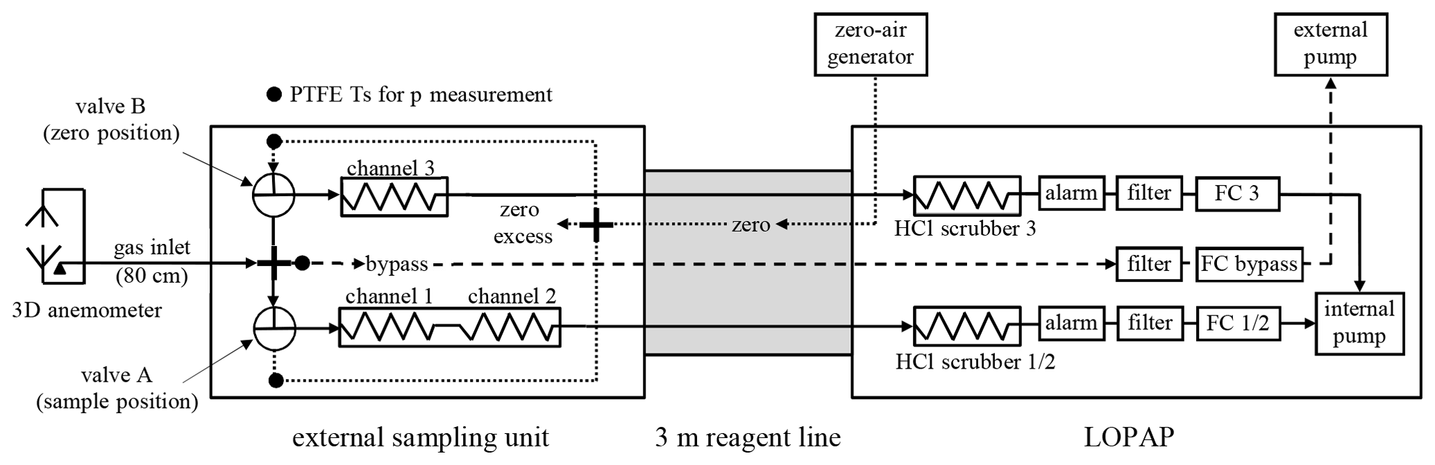
For the additional implementation of the REA gas inlet (see next section) a new compact sampling unit was developed (see Fig. S1). In addition, the temperature-controlled reagent line was modified, housing nine liquid lines for the three channels (see Fig. S2) and additional gas lines for the bypass and the zero-gas generator (see Fig. 1). In the LOPAP instrument an additional 2 L min⁻¹ mass flow controller (Bronkhorst), a second HCl-scrubber and a security bottle (“alarm”) were installed for the new channel 3. In addition, a 5 L min⁻¹ mass flow controller (Bronkhorst) and an external membrane pump (KNF) were installed to control the bypass flow of the REA gas inlet (see Fig. 1). As well as this, the liquid flow scheme was also adopted to the new three-channel LOPAP (see Fig. S2). Since the internal peristaltic pump (Ismatec) has only 16 channels, from which 13 are already used in a normal two-channel LOPAP, an additional external four-channel peristaltic pump was necessary to remove the bubble-containing waste of the three channels from the glass T-junctions behind the stripping coils (see Fig. S2).

3.2 The REA gas inlet

For the REA method two separate channels are probed with updrafts and downdrafts by switching two valves, which are placed in the external sampling unit (see Figs. 1 and S1). Caused by its size and to minimize its impact on the turbulence measurements of the ultrasonic anemometer (CSAT3B, Campbell Scientific Inc.) the external sampling unit is installed ∼80 cm leeward to the centre of the anemometer (see Fig. S4). The ∼80 cm long PFA inlet line (4 mm i.d.) from the anemometer to the external sampling unit was covered by aluminium foil to minimize artificial photochemical formation of HONO (Zhou et al., 2002b). The inlet was protected against rain by a small cone (see Fig. S4, right; 3 cm diameter) and was positioned below the anemometer, slightly shifted to the lee side, following the recommendations of Kristensen et al. (1997). The use of an inlet line is normally not recommended for the LOPAP technique but was necessary to spatially separate the anemometer and the external sampling unit. Thus, small positive artefacts could be possible by heterogeneous dark formation of HONO in the inlet. However, this should not affect the HONO fluxes, which are calculated from the concentration difference of updrafts and downdrafts and not from the absolute HONO levels (see Eq. 3).

During REA measurements each channel of the instrument is fed for a certain time with ambient air, depending on the vertical wind direction. In contrast, for closed valves, when the vertical wind is too small during deadband conditions or during zero measurements, the LOPAP channels are operated by zero air. Therefore, fast (<12 ms response time) three-way valves (miniature inert PTFE isolation valves series 1, Parker Hannifin Corp., USA) were used to feed the stripping coils either with ambient air or with zero air. By using a PTFE cross (BOLA, 1.6 mm i.d.), the sample air from the PFA inlet line is directed to the two valves (see Figs. 1 and S1). Since the inlet line has to be flushed by ambient air during the deadband to minimize heterogeneous HONO formation, the remaining open port of the PTFE cross is connected to the bypass line (see Figs. 1 and S1) for which a flow rate of 2.65 L min⁻¹ (298.15 K, 101 325 Pa) is used in the present study.

The zero-air lines of both channels are connected via a stainless-steel cross (Swagelok, Ohio) to the main zero-gas line. The remaining open port of the cross is used for the excess vent of the zero air. Zero air was obtained from a home-made zero-air generator (see Fig. S4), where compressed ambient air by a membrane pump is pushed through a particle filter, a flow controller (Bronkhorst: 5 L min⁻¹), two cartridges filled with active charcoal and active charcoal coated with Na₂CO₃, and another particle filter. The zero-air flow is adjusted slightly higher than the gas flow of both channels, when both valves are closed during deadband and zero-air periods. The dilution of the ambient air during REA measurements is later corrected for during data evaluation (see Sect. 4.1).

During REA measurements both valves switch between ambient and zero air. For both measurement conditions a constant air flow through the stripping coil is assumed to correctly calculate the dilution of the ambient air in each channel during the averaging interval. However, constant air flow can only be obtained when the pressure at the inlet of the stripping coil is independent of the valve position. Initially, this was not the case since the pressure at the inlet of the stripping coil was lower during ambient air compared to zero-air measurements. This was caused by the longer inlet line and the higher gas flow rate including sample and bypass flow compared to the flow rate in the shorter zero-air line from the stainless-steel cross (= ambient pressure) to the valve (see Fig. 1). Therefore, during first test measurements with variation of the valve switching times (see Sect. 4.2) systematic and significant variations of the resulting dilution-corrected HONO concentrations were observed. Since the flow controllers of the two channels (valve A: channels 1+2; valve B: channel 3) are installed inside the LOPAP instrument and are connected via particle filter, security bottle, HCl-scrubber and a gas line more than 3 m long to the stripping coil (see Fig. 1), the flow rates were changing after switching the valves until new pressure equilibria were reached in the volumes from the stripping coil to the flow controller. This problem appeared particularly with short valve switching periods as applied during REA measurements.

To avoid this inlet pressure problem, first, the diameter of the PFA inlet line was increased from 1.6 mm i.d. to 4 mm i.d., decreasing the depression at the inlet of the stripping coils. Second, the length of the 1.6 mm i.d. PFA zero lines from the stainless-steel cross (= ambient pressure) to the valves was increased until the pressure at the valve was independent of the valve position (depression similar during ambient and zero measurements). To adjust the pressure in the REA inlet, three PTFE T-junctions (Bola, 1.6 mm i.d.) were installed at the end of the two zero-air lines at the valves and at the inlet of the bypass line (see Figs. 1 and S1). After removing the blind caps from the Ts, the pressure can be measured by a pressure gauge (Baratron 0–1000 hPa). For fine adjustment of the pressure, the bypass flow rate is adjusted, which only has an influence on the depression during ambient air measurement, but not during zero-air supply (see Fig. 1). For the fine adjustment of the pressure during deadband – here both channels are operated under zero air and the pressure must be similar at the inlet of both coils – the sample flow rates of both channels were slightly varied. The exact adjustment of the inlet pressures at the two stripping coils under the different operation conditions was the largest problem during the development of the REA-LOPAP system. Only after this was solved were successful REA measurements possible.

3.3 REA data logging and valve controlling software – PyREA

Data logging, processing of the anemometer raw data, and control of the REA valves and measurement cycles was performed with a control program, PyREA, developed primarily in the Python programming language. The applied REA theory and the implemented formula are explained in Sect. 2. Specifically, Eq. (5) was used to calculate b_w, which is later used to calculate the HONO flux by Eq. (3). Details of the program are explained in Sect. S3 in the Supplement.

The software was operated on a single board computer (Raspberry Pi, version 3 B+). The user interface of PyREA was accessed via a Secure Socket Shell (SSH) connection from the LOPAP data acquisition computer, which allows the REA parameters to be controlled (e.g. mode switching times). Here, the sequence of REA, zero and parallel ambient measurements can be adjusted to run automatically (“auto-REA mode”). During REA measurements, each valve switches between ambient air and zero air, controlled by the vertical wind signals from the anemometer and the width of the deadband. Regular zero measurements (both valves are closed) are necessary for the LOPAP technique (Heland et al., 2001), and regular parallel ambient measurements (both valves are open) were used to improve the precision between the two channels for the updrafts and downdrafts.

In the software the different lag times when switching from ambient air measurements to deadband (sample + bypass inlet flow) or from deadband to ambient measurement (only bypass inlet flow) can be adjusted for the REA measurements. Besides the flow rates and the volume of the inlet (10.1 cm³), the response time of the valves (12 ms) and the delay of the anemometer (95 ms: only first 10 ms sample of each 100 ms interval is provided by the anemometer) also have to be considered. The lag time is calculated by the variable inlet residence time minus the anemometer delay time and the valve response time.

Alternatively, the valve can also be operated manually by the graphical interface (GUI), which is necessary during adjustment of the pressure in the REA inlet for example (see Sect. 3.2). Furthermore, different test modes were implemented in the software, which were used during the development of the REA system. For example, artificial anemometer data can be simulated for tests inside the laboratory (test mode: simulate_anemometer), or the valves can be operated in a pre-defined continuous sequence (test mode: valve_function_test). The latter was used to test the dilution correction for variable valve switching times (see Sect. 4.2).

3.4 Laboratory set-up

To test the new REA system in the laboratory and in front of the facade of the laboratory building, a mobile laboratory rack was developed, on which all components of the system were installed. The external sampling unit and the anemometer were fixed on an aluminium arm with a similar geometry compared to the field set-up (see Fig. S4 left). Through an opening in an exchanged window element of the facade of the laboratory the external sampling unit and the anemometer could be moved outside of the building, with the rack with the LOPAP being inside the laboratory (see Fig. S4 right). The opening could be closed by two PVC plates with smaller holes for the aluminium arm, the insulated reagent line from the external sampling unit to the LOPAP instrument and the cables from the anemometer. This set-up allowed measurements to be started inside the laboratory, which was necessary for gas flow rate measurement during calibration for example. Then, with the running instrument the set-up could be changed to ambient test measurements in front of the facade of the building.

3.5 Field set-up in Melpitz

For the field campaign in Melpitz a field rack was available, which was already used in our former gradient measurements in Grignon, France (Laufs et al., 2017). For the present study, the field rack was upgraded with an external air conditioning system with 1 kW cooling power (SoliTherm Outdoor, Seifert Systems GmbH; see Fig. S5, left) to ensure constant temperatures inside the rack also under sunny summertime conditions.

The field campaign took place at the field site Melpitz (12.9277^∘ E, 51.5255^∘ N, 86 m NN), which is operated by the TROPOS institute in Leipzig, Germany, and is used as a regional station by the Global Atmosphere Watch (GAW) program. The station is located on grassland, which is surrounded by farmland. The nearest buildings of the small village Melpitz are located ∼360 m to the east of the station. The terrain is uniform and even, which ensures horizontal homogeneity of the flow field and makes the site well suited for micrometeorological measurements. The railroad tracks from the Leipzig–Torgau line and the state road 87 are located ∼1 and ∼1.5 km north of the station, respectively. The next buildings in the south-westerly direction are from the village Klitzschen at ∼1.5 km distance. A small district road connecting Melpitz and Klitzschen is located ∼400 m south of the station. The REA system was installed ∼80 m west of the TROPOS measurement containers, and because of typical south-westerly winds no influence of the station on the turbulence and HONO measurements is expected. At ∼130 m distance to the west there is a single open line of smaller trees and bushes (see Fig. S5, right) which is converging to ∼70 m to the south of the field site. The REA sampling unit and the anemometer were installed on a small mast in the south-westerly direction (220^∘) to the field rack facing the expected main wind direction and thus minimizing the influence of the field rack to the turbulence measurements (see Fig. S5). The centre of the anemometer was located at ∼200 cm height above the grass surface. To avoid turbulence disruptions by the inlet line, the gas inlet was slightly shifted to the lee side (8 cm) and placed below the anemometer at ∼170 cm height, following the recommendations of Kristensen et al. (1997). During the campaign, regular parallel ambient measurements of 30 min were used after two measurement cycles (one measurement cycle consists of a 240 min REA period and a subsequent 30 min zero period). As filter for the deadband (see Sect. 2) values of K=0.9 and K=0.6 were used during the campaign.

Besides the HONO flux measurements, also the actinic flux and the photolysis frequencies J(NO₂), J(HONO) and J(O¹D) were determined by a spectroradiometer with a cooled CCD detector and a 2π collector (Meteoconsult) on the roof of one measurement container at the main TROPOS station. In addition, NO and NO₂ concentrations were measured at the TROPOS station by the chemiluminescence technique (Eco Physics, CLD 770 AL) with a blue-light NO₂ converter (homemade, University of Wuppertal). The instrument was calibrated 6 times during the campaign with an NO calibration gas (Messer 450±10 ppb) for which the NO₂ converter efficiency was also determined to be (50.4±0.7) % by an O₃-titration unit (Anysco GPT). For the NO_x measurements the common gas inlet of the standard NO_x instrument from the TROPOS station was used, the data of which were not considered here, due to its higher precision errors and detection limit.

Additionally, data for nitric acid (HNO₃) measured by a MARGA instrument (Stieger et al., 2018), wind direction and speed, temperature, and relative humidity from the TROPOS station were used for data evaluation.

4 Laboratory tests

With the laboratory set-up (see Sect. 3.4) test measurements were performed inside the laboratory and at the facade of the laboratory building to develop a data evaluation procedure (Sect. 4.1) and to validate the dilution correction for variable valve switching times (Sect. 4.2).

4.1 Data evaluation

During flux measurements simultaneous data from the data acquisition system on the LOPAP computer (HONO raw absorbance) and from the PyREA software on the Raspberry Pi (three-dimensional wind speed (u, v, w), air temperature (T) and valve switching data from the REA inlet) are collected. The software also calculates wind direction and wind speed, as well as the REA parameters b and σ_w.

For both data logging systems 30 s data are recorded, for which the REA data are calculated both as 5 and 30 min running averages (see Sect. S3), which are first combined in one data file. Since the time correction of the LOPAP data (lag time between sampling and dye detection) shows a continuous shift caused by a slight reduction of the liquid flow rates of the peristaltic pump, the time-corrected 30 s LOPAP data are synchronized to the 30 s REA data.

The LOPAP data are evaluated similarly to the usual procedure (see Heland et al., 2001; Kleffmann et al., 2002). Here, time response (time for 10 %–90 % increase in the signal: ∼5 min) and time correction (time to 50 % change: ∼16 min) are determined from the raw data ($\log (I_{\mathrm{ref}}/I)$; see Heland et al., 2001) and the time stamps of the PyREA software. Furthermore, the raw absorbance of only the zero measurements is described by polynomials as a function of time, which are subtracted from the raw absorbance data, leading to zero-corrected data in the form required by Lambert–Beer's law ($\log (I_{\mathrm{0}}/I)$), which should be zero in between their precision errors during all zero measurements. Next, from the calibration of the instrument by a nitrite standard in R1 (0.01 mg L⁻¹) under zero air, the slopes of the analysis functions (ppt ABS⁻¹) are determined for all three channels, from which the diluted concentrations are calculated by multiplying with the zero-corrected absorbance data (see Fig. 2).

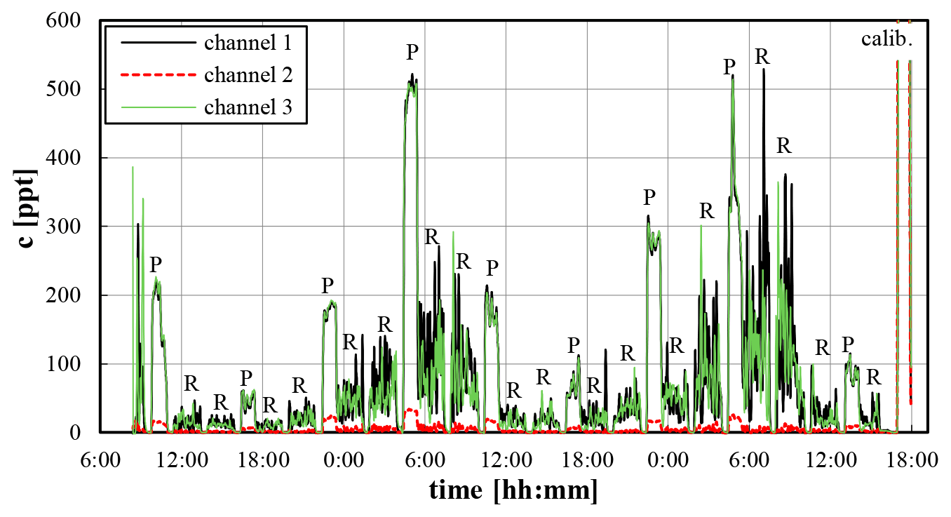
Figure 2 Mixing ratios (30 s raw data) of the three LOPAP channels during test measurements at the university of Wuppertal. Periods marked with “P” show undiluted parallel ambient measurements (60 min), while the REA measurements (dilute samples) are signed by “R” (120 min). In between, regular zero measurements (30 min) are performed.

Since HONO fluxes are determined from small concentration differences between updrafts and downdrafts (see Eq. 3), high precision is required for channels 1 and 3. For validation of this requirement, regular parallel ambient measurements are performed by the system, for which both channels measure exactly the same air masses. For the test campaign shown in Fig. 2 excellent agreement between both channels was observed for all parallel ambient measurements (periods marked by “P”). In addition, a high correlation of both channels (R²=0.9986), excellent agreement (slope: 0.9982±0.0014) and an insignificant intercept of 2 ppt within the quantification error limit were observed. Since the ratio channel 1 $/$ channel 3 showed a small but significant variation with time, the ratio was parameterized as a function of time for later harmonization of both channels (see below).

Next, the concentrations of all three channels were corrected for dilution during the REA measurements by using the valve switching statistics recorded by the PyREA program for each averaging interval. Depending on the vertical wind direction, each channel of the instrument collects ambient air only for a fraction of the averaging interval (e.g. one-third). For the rest of the time (i.e. two-thirds for the example), when the instrument is in the dead band, or when the other channel is sampling ambient air, zero air is sucked into the stripping coil. Thus, the measured HONO concentration reflects a diluted sample, which is corrected for by the inverse of sampling fraction (i.e. by multiplication by a factor of 3 in the example). The 5 min moving average data of the valve switching statistics were used for this correction due to the similar physical time response of the LOPAP instrument (see Sect. 3.1). For channels 1 and 2 the valve switching statistics of valve A and for channel 3 the valve switching statistics of valve B were used (see Fig. 1).

Then, the dilution-corrected concentrations were harmonized by the parameterization derived from the parallel ambient measurements (see above). Since it is unclear which of the channels measures correctly, all channels were corrected only by half of the ratio (channel 1 $/$ channel 3) determined during the parallel ambient measurements, for which channels 1 and 2 were divided and channel 3 multiplied by this ratio, respectively. The interference channel 2 was harmonized in the same way as channel 1, since both channels sample the same air mass (see Fig. 1). However, caused by the typical small signals in channel 2 (∼10 % of channel 1), any errors in the harmonization of channel 2 (typically only 1 %–2 % correction) will not significantly affect the accuracy of the HONO data (i.e. by only 0.1 %–0.2 %, much smaller than the precision error of the instrument).

Similar to the usual LOPAP data evaluation (see Heland et al., 2001; Kleffmann et al., 2002), from the corrected and harmonized concentrations in channel 1 and 3 (measuring HONO + interference) the dilution-corrected and harmonized concentrations in channel 2 (measuring only the interference) were subtracted. To consider the sampling efficiency of the stripping coils for HONO, first, the signals of channels 1 and 3 are divided by the sampling efficiency of 0.996 to account for the loss of HONO by incomplete sampling. Second, the loss of HONO to the interference channel 2 (channel 1 ×0.004) is subtracted from channel 2 and only the remaining interference is subtracted from the signals in channels 1 and 3.

From the resulting HONO concentrations of both channels an average HONO concentration can be calculated, weighted by the fractions of sampling times of both channels during the 5 min averaging periods (see Fig. 3). This average HONO concentration determined by the REA system should be similar to concentrations determined with a normal LOPAP instrument. Deviations caused by missing data during the deadband are considered small, since small concentration differences between the updrafts and downdrafts are expected during the low-turbulence deadband conditions. This is confirmed by the non-significant variations of the HONO concentrations when the system switches from parallel ambient measurements (continuous sampling of ambient air in both channels) to REA measurements (see Fig. 3). Thus, in addition to the HONO fluxes (see below) HONO concentrations can also be determined, similar to a normal LOPAP instrument. It should be mentioned again that the average HONO concentration determined by the REA-LOPAP system may be affected by systematic artificial HONO formation in the inlet line. However, caused by the high air flow rate of 3.7 L min⁻¹ (sum of bypass and sample flow rates of 2.65 and 1.05 L min⁻¹, respectively) and the short PFA inlet line (80 cm) covered by aluminium foil, artificial heterogeneous HONO formation in the dark inlet during the short residence time of 160 ms is considered small. An intercomparison with a normal LOPAP instrument without any inlet line is required to further confirm this assumption in the future.

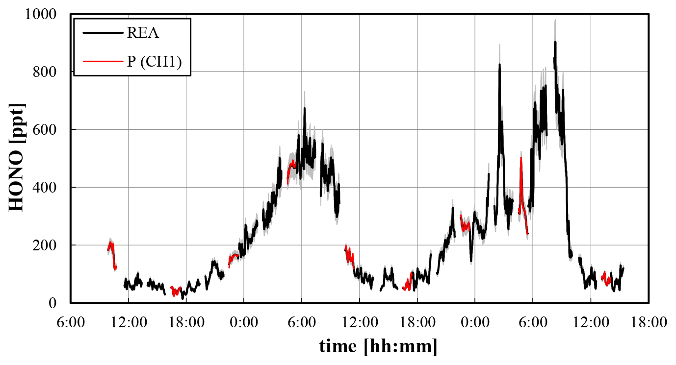
Figure 3 Weighted average HONO concentration determined from both channels during REA measurements (REA) and HONO concentration from channel 1 during parallel ambient measurements (P (CH1)) for the test campaign at the university of Wuppertal (30 s data, 5 min running mean). The grey shaded area reflects the accuracy of the data.

To validate that the applied interference correction using a three-channel system is applicable, the assignment of the updrafts and downdrafts to the two physical LOPAP channels is regularly alternated after each parallel ambient measurement by the PyREA software. In the mode “up”, channels 1 and 2 (double stripping coil) are fed with ascending air and channel 3 (single stripping coil) measures the descending air, while the assignment is inverted in the mode “down”. Thus, the relative interference can be determined for both air masses. For the test measurements at the university of Wuppertal average interferences of (8.4±2.4) % and (7.5±4.3) % were determined for the updrafts and downdrafts, respectively. These values are similar within their combined variability. Even if the difference was considered, this would only affect the HONO concentrations in channel 3 by less than ±1 %, which is lower than the precision error. In the case of potential larger differences of interferences in other campaigns, the data from channel 3 could be corrected considering the measured average ratio interference${}_{\mathrm{up}}/$ interference_down depending on the mode (“up” $/$ “down”) applied.

Besides the validation of the interference correction method, the regularly changing assignment of the air masses to the two physical channels of the REA LOPAP has to be considered for the determination of the HONO flux, which is calculated from the concentration difference of both channels ($\mathrm{\Delta }\mathrm{HONO}={\mathrm{HONO}}_{\mathrm{up}}-{\mathrm{HONO}}_{\mathrm{down}}$). Due to the requirement of the REA method (see Sect. 2) 30 min running means of ΔHONO are calculated. By using the measured ambient pressure and the air temperature ΔHONO is converted from mixing ratios [ppt] to concentrations [molecules m⁻³]. According to Eq. (3) (see Sect. 2) HONO fluxes [molecules m⁻² s⁻¹] are obtained by multiplication of ΔHONO with 30 min running mean values of b [–] and σ_w [m s⁻¹] obtained from the PyREA software. The fluxes determined during the test measurements in Wuppertal were, however, not further considered, caused by the distorted turbulence in front of the facade of laboratory building.

4.2 Variation of valve switching periods

After correctly adjusting the pressure in the REA inlet (see Sect. 3.2) the valve switching periods were systematically varied by using the PyREA test mode valve_function_test (see Sect. 3.3) at constant HONO concentrations by using a pure HONO source (Villena and Kleffmann, 2022). A sequence of zero (both valves closed) and parallel ambient measurements (both valves open) and subsequent valve switching periods was performed, for which constant valve switching times of 1, 2, 3 and 4 s were applied for the periodically switching valve positions (1) up, (2) deadband, (3) down and (4) deadband, respectively. Caused by the chosen valve switching sequence, the HONO concentration is diluted by exactly a factor of 4 in both channels during these experiments (see Fig. 4: “P” and “xs”).

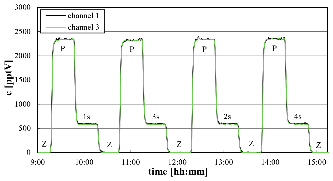
Figure 4 HONO mixing ratios during test measurements using a pure HONO source and variable valve switching times (30 s data). “Z”: zero; “P”: parallel ambient measurements; “xs”: valve switching experiments with constant periods for up, down and deadband measurements (each with 1, 2, 3, 4 s using the sequence up, deadband, down and deadband; dilution by a factor of 4 each).

For the parallel ambient measurements an excellent agreement between channels 1 and 3 was again observed, with an average ratio (channel 1 $/$ channel 3) of 1.002±0.006. Thus, no further harmonization of the two channels (see Sect. 4.1) was performed for the short measurement period applied. For the valve switching test the expected dilution by a factor of 4 could be confirmed in both channels. Here, a mean ratio (channel 1 $/$ channel 3) for the dilution-corrected data of 1.023±0.012 was observed. The small deviation of 2.3 % is in between the precision error of the instrument considering the applied dilution correction and is independent of the chosen switching time interval. In addition, no significant differences between the HONO data during parallel ambient measurements and the dilution-corrected data during the valve-switching experiments were observed. For the average ratios (parallel ambient measurements $/$ valve switching) values of 0.984±0.015 and 1.005±0.017 were observed for channels 1 and 3, respectively. Thus, first, the agreement between both channels is independent of the valve switching period, and second, the dilution is correctly determined by the system, which is the basic requirement for REA measurements.

4.3 Flux errors

Errors in the fluxes were determined by error propagation of the accuracy of the LOPAP instrument (7 %), estimated uncertainty in the harmonization function derived from the parallel ambient measurements (5 %), the precision errors of the 30 min values of ${\mathit{\sigma }}_{\mathrm{w}}/b_{\mathrm{w}}$ (standard deviation of the 5 min running mean data) and the HONO concentration difference ΔHONO. For the latter the precision of the LOPAP instrument (2.2 % for the campaign in Melpitz), the detection limit (0.8 ppt for the campaign in Melpitz) and the dilution ratios during REA measurements were considered for all channels of the instrument by error propagation. Possible uncertainties introduced by the choice of calculation method of the b coefficient (see Sect. 2) were not considered in error propagation, but b values determined by different methods were compared to assess their quality (see Sect. 5.1).

Further systematic errors in REA fluxes can arise from insufficient fulfilment of the prerequisites and assumptions, which underlie all micrometeorological flux measurement methods (see for example Baldocchi et al., 1988). Therefore, results of field campaigns are often assessed by evaluating turbulence development (see Sect. S7 for the field campaign in Melpitz). Furthermore, the correct determination of the time lag between the change of the sign of the vertical wind and the actual switching of the valves is vitally important for the attribution of the sampled air to the two measurement channels. Imprecise time lags can cause significant errors on determined fluxes, especially in REA systems with long inlet lines (Moravek et al., 2013). The time lags of our system depend mainly on the sample flow rates and were quite short, caused by the short inlet line and the high gas flow rate. Due to the different air flow rates in the inlet, different time lags when switching from ambient air to deadband (57 ms) or from deadband to ambient air (123 ms) were individually considered (for details see Sect. 3.3). Therefore, errors of the calculated fluxes caused by imprecise time lags are expected to be negligible for the present application.

5 Field campaign in Melpitz

5.1 General observations

The field campaign took place during the period 27 September to 2 October 2020 after a period of strong rain. During the campaign the weather was dry and sunny again, with a completely clear sky on 1 October 2020. The temperatures varied from 3.5 ^∘C during the night up to 20 ^∘C during the early afternoon. The relative humidity was in the range 50 %–60 % during early afternoon and increased to 100 % during late night to early morning (see Fig. S6). The turbulence was well developed between 08:30 and 16:30 LT (local time), while low wind speeds and stable stratification of the atmosphere caused higher relative errors of the HONO fluxes in the evenings and during night-time (see Sect. S7).

Caused by the requirements of the REA method (see Sect. 2), 30 min averages of the data of all instruments were used for the data evaluation. In addition, only those periods were used for which data from all instruments were available. As well as a short failure of the data logger of the spectroradiometer on 29 September 2020, during calibrations of the NO_x instrument and during zero and parallel ambient measurements of the LOPAP also no flux data were available. Finally, data with wind directions from north-north-east (340–50^∘) were also not considered, in order to avoid the potential turbulence disturbance of the field rack.

The NO_x concentrations were relatively high for this rural measurement site. NO decreased from up to 12 ppb in the morning to the detection limit of the instrument (30 ppt) in the late afternoon. NO₂ showed smaller variability with mixing ratios in the range 2–10 ppb (see Fig. S6). HONO levels varied in the range 2–280 ppt (see Fig. 5) but did not show a typical urban diurnal variation with high concentrations during night-time, decreasing after sunrise to a minimum in the late afternoon (see for example Fig. 3 at the University of Wuppertal). Especially for 30 September to 2 October 2020 in Melpitz the HONO concentrations were decreasing during the night and then increased again in the morning with a maximum before noon. Since the NO_x levels were also high at that time (see Fig. S6), the late morning peaks may be explained by delayed arrival of polluted air masses, e.g. from the morning rush hour in Leipzig.

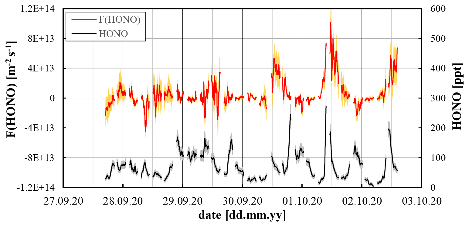
Figure 5 HONO mixing ratios and HONO fluxes (30 min running mean data) in Melpitz. The grey and orange shaded areas reflect the accuracy of the data.

Interferences were determined for both the updrafts and downdrafts by regular changing of the allocation of the air masses to the physical channels of the instrument. Mean values of interference${}_{\mathrm{up}}=(\mathrm{7.0}\pm \mathrm{5.5})$ % and interference${}_{\mathrm{down}}=(\mathrm{8.0}\pm \mathrm{7.8})$ % were determined, which were similar in between their combined variability. In addition, similar concentration dependencies of the interferences were observed, which show decreasing interferences with increasing HONO levels, similar to other LOPAP measurements (see Fig. 5 in Kleffmann and Wiesen, 2008). Thus, the applied interference correction, using the interference data only from one channel for both air masses is considered accurate enough to determine HONO fluxes by the three-channel REA-LOPAP system.

The comparison of three methods for calculation of the b values (see Sect. 2, Eqs 4–6) during the field campaign in Melpitz using two K values of 0.9 and 0.6 (see Eq. 2) showed very good agreement, when data from 08:30 to 16:30 LT were used. The average daytime b_w (Eq. 5) was 0.35±0.02 for K=0.9 and 0.43±0.03 for K=0.6. These values are in good agreement with daytime values of b_Proxy determined with the sonic temperature as proxy scalar (see Eq. 4) of 0.34±0.06 and 0.38±0.05, respectively. Finally, when a typical experimentally determined value of b₀=0.56 (Katul et al., 1996; Baker et al., 1992) was used in Eq. (6), the parameterized b_model values were 0.36 and 0.39, respectively.

5.2 HONO fluxes

The HONO fluxes showed a clear diurnal trend with low fluxes during night-time and a maximum around noon. The positive daytime fluxes were increasing to the end of the campaign (see Fig. 5), which is explained by the previous strong rain period and the slowly drying soil surfaces during the following dry period. Since HONO is very soluble in water – particularly when in contact with slightly alkaline soil surfaces – high HONO emissions were initially prevented by the wet surfaces and increased only when the soil surfaces dried. During the last days a clear diurnal flux profile was observed showing low, partially negative fluxes (deposition) during night-time and higher positive fluxes (emission) around noon. During the campaign, the HONO fluxes varied in the range $-\mathrm{4}\times {\mathrm{10}}^{\mathrm{13}}$ to $+\mathrm{1.0}\times {\mathrm{10}}^{\mathrm{14}}$ molecules m⁻² s⁻¹ (see Fig. 5).

For a better description of the general trends, a mean diurnal profile was calculated from the 30 min mean data of all instruments for the last four days, which is shown in Fig. 6. As already described above for the single days, low and partially negative fluxes were observed during night-time, which were increasing to $\sim \mathrm{4}\times {\mathrm{10}}^{\mathrm{13}}$ molecules m⁻² s⁻¹ during daytime around noon.

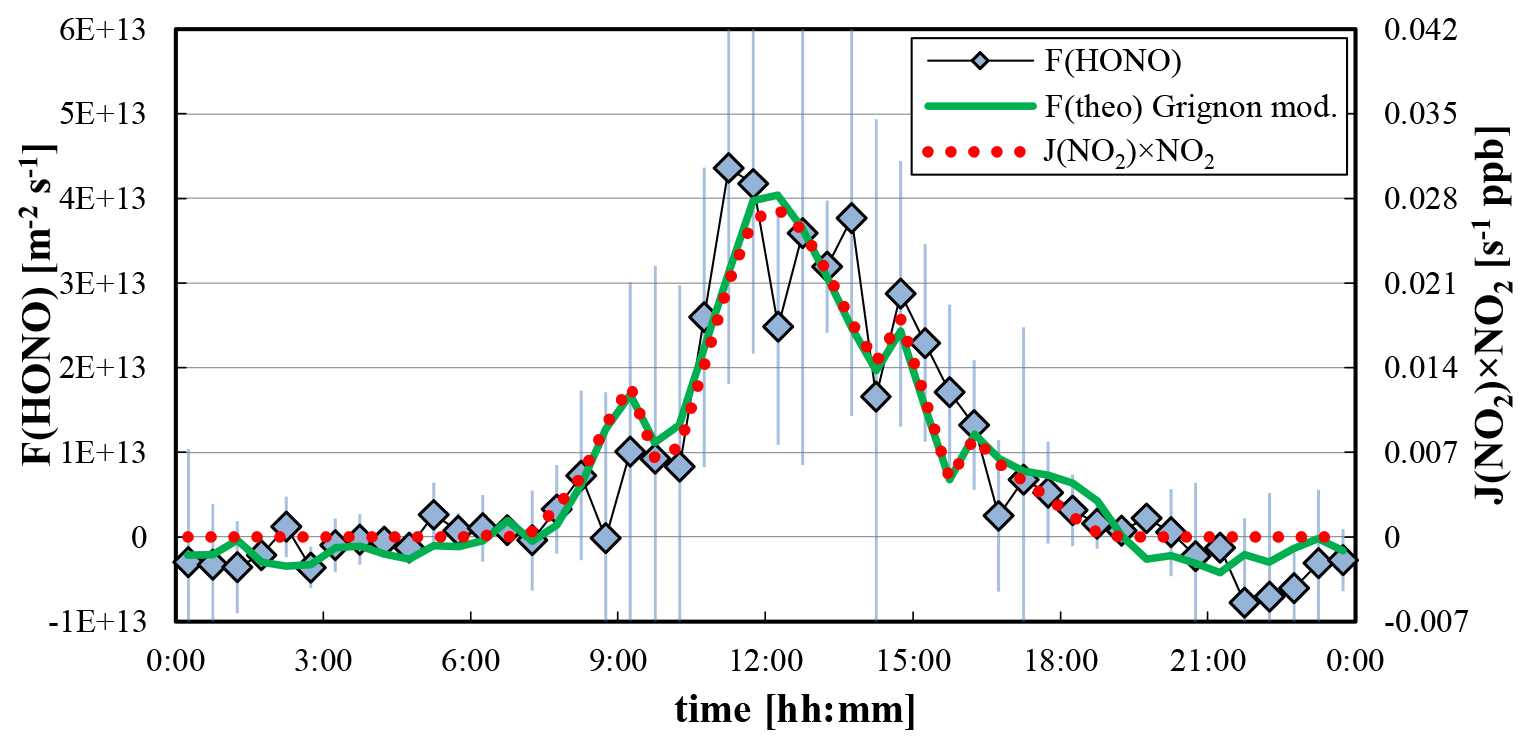
Figure 6 Average diurnal day of the HONO fluxes of the last four days of the campaign in comparison to a modified parameterization from former gradient measurements in Grignon, France (Laufs et al., 2017); see Sect. 5.4. Error bars represent the standard deviation of the HONO fluxes of the 4 d. In addition, the scaled product J(NO₂)⋅[NO₂] is also shown.

In other studies, very similar diurnal trends of the HONO flux were observed, which are following the diurnal trend of the radiation (Ren et al., 2011; Zhou et al., 2011; Zhang et al., 2012; Laufs et al., 2017). However, the average maximum HONO fluxes of typically $\sim \mathrm{1}\times {\mathrm{10}}^{\mathrm{14}}$ molecules m⁻² s⁻¹ were higher by factors of 2–3 in these studies compared to the data shown in Fig. 6. Only during the BEARPEX 2009 campaign (Ren et al., 2011) and in a forest clearing (Sörgel et al., 2015) were lower daytime HONO fluxes observed compared to the present study. Reasons for the low HONO fluxes in Melpitz may be the solubility of HONO on the wet surfaces, as mentioned above, or lower nitrogen content in the non-fertilized soils of the Melpitz grass land compared to the other studies. In recent flux studies using twin open-top soil chambers in China, HONO fluxes up to 2 orders of magnitude higher were observed shortly after strong fertilization of the soil surfaces (Tang et al., 2019; Xue et al., 2019).

5.3 Potential HONO formation mechanisms

To identify potential HONO formation mechanisms, the diurnal averaged HONO fluxes were plotted against different potential precursors and parameters. The best correlation was observed between the HONO flux and the product J(NO₂)⋅[NO₂] (R²=0.86; see also Fig. 6), which is in excellent agreement with REA flux measurements during the CalNex 2010 campaign (Ren et al., 2011) and gradient measurements in Grignon, France (Laufs et al., 2017). The results are also in good qualitative agreement with field studies, in which the daytime source of HONO was determined by the photostationary state (PSS) approach. In these studies, good correlations of the HONO source were observed with radiation (J(NO₂) or irradiance) and/or the product of radiation ⋅[NO₂] (Vogel et al., 2003; Elshorbany et al., 2009; Sörgel et al., 2011; Villena et al., 2011; Wong et al., 2012; Lee et al., 2016; Meusel et al., 2016). These results point to a HONO formation mechanism identified in the laboratory by the photosensitized conversion of NO₂ on organic surfaces, e.g. on humic acids (George et al., 2005; Stemmler et al., 2006, 2007; Bartels-Rausch et al., 2010; Han et al., 2016a, b, 2017; Yang et al., 2021a).

Based on laboratory and field studies, other HONO sources are also discussed, for example the photolysis of nitrate $/$ HNO₃ adsorbed on surfaces (Zhou et al., 2003, 2011), which requires shorter UV wavelengths compared to the photosensitized conversion of NO₂ (see above). Unfortunately, nitrate concentrations on the soil and leaf surfaces were not measured in the present study. However, it is expected that the maximum of this HONO source typically appears in the afternoon, since HNO₃ mainly forms by the oxidation of NO₂ by OH radicals in the gas phase during daytime, followed by the dry deposition of gaseous HNO₃ to ground surfaces. The diurnal maximum of gas-phase HNO₃ in the afternoon was confirmed for the present field campaign (see Fig. 7), and an even later maximum is expected for deposited HNO₃ on ground surfaces. Since the highest HONO fluxes were observed around noon (Fig. 7), the main HONO formation by nitrate $/$ HNO₃ photolysis is unlikely for the present field site. In addition, the correlation of the HONO flux with the product J(O¹D)⋅[HNO₃] (R²=0.60) was weaker compared to the product J(NO₂)⋅[NO₂] (R²=0.86). Here J(O¹D) was used for the nitrate $/$ HNO₃ photolysis because of the expected similar spectral ranges of the action spectra of HNO₃ and O₃ in the atmosphere (290–330 nm). Finally, only low photolysis frequencies J(HNO₃) of adsorbed nitrate $/$ HNO₃ were observed in recent laboratory studies (Laufs et al., 2017; Shi et al., 2021), confirmed by a field study, for which the nitrate photolysis was also excluded as a main HONO source in the atmosphere (Romer et al., 2018).

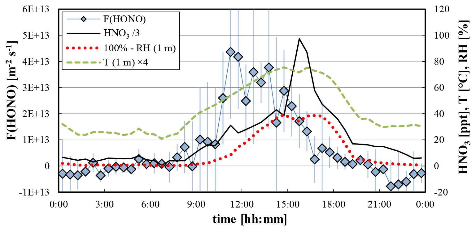
Figure 7 Average diurnal profiles of the HONO flux, HNO₃ mixing ratio, and the relative humidity (100 % − RH) and temperature of the air at 1 m height. Error bars represent the standard deviation of the HONO fluxes of the four days.

The microbiological formation of nitrite in soils was proposed in laboratory studies as a further HONO daytime source (Su et al., 2011; Oswald et al., 2013). For this HONO source a strong negative humidity dependence was observed, which was explained by the solubility of HONO in soil water. In addition, the temperature of the upper layer of the soil was identified as an important parameter, for which the HONO emissions should increase with the soil temperature. Unfortunately, the soil water content and temperature were not measured in the present field campaign. Due to the heat capacity of the soil, it is expected that the diurnal profiles of both parameters follow those of the air temperature and humidity. Since the highest air temperature and lowest relative humidity were observed at 15:00–17:00 LT (see Fig. 7), the maximum of a potential biological soil source is expected at a similar or even later time of the day. In contrast, the highest fluxes were observed around noon near the maximum of the solar radiation (see Fig. 6). In addition, low correlations of the HONO fluxes were observed with the inverse of the relative humidity at 1 m height (R²=0.26), with the difference (100 % − RH) (R²=0.31) and with the near ground (1 m) air temperature (R²=0.46), again contradicting a main HONO source by microbiological formation of nitrite in the soil. In a field study by the group, which originally proposed the biological source, a strong correlation of the HONO emissions with radiation was also observed and, therefore, their former laboratory results could not be confirmed (Oswald et al., 2015).

A further proposed daytime HONO source is the replacement of night-time adsorbed HONO $/$ nitrite by strong acids on soil surfaces, for example after deposition of HNO₃ (Donaldson et al., 2014; VandenBoer et al., 2014, 2015). However, this mechanism also seems to be not very plausible in the present study because of the main formation mechanism of HNO₃ and its diurnal mixing ratio profile, with a maximum in the late afternoon (see Fig. 7). Caused by the subsequent dry deposition of HNO₃, an even later maximum is expected for the HONO source by acid replacement, in contrast to the observed HONO flux profile.

In a very recent study at the same measurement site in Melpitz, HONO emissions by evaporation of nitrite containing dew water was proposed (Ren et al., 2020). The nitrite was explained by the dry deposition and solubility of HONO in dew water during the preceding night but could not be confirmed by parallel dew and gas-phase measurements. At first glance, this mechanism could be also plausible for the present field study, since the increase in the HONO concentration in the late morning on 30 September to 2 October 2020 (see above) appeared at the same time, when the relative humidity decreased from saturation values (100 % RH), indicating the start time of dew evaporation. At the same time also the average HONO fluxes started to increase (see Fig. 7). Dew measurements were not available for the present field study to confirm the proposed mechanism, which is, however, ranked unlikely here, because of the smaller integrated deposition of HONO during the night compared to the positive daytime fluxes (see Fig. 6). Integrated night-time deposition of HONO of only 5.9×10¹⁶ molecules m⁻² was determined for the average day, much smaller than the integrated average daytime HONO emissions of 7.0×10¹⁷ molecules m⁻². Thus, even when assuming an unreasonable quantitative re-emission of night-time deposited HONO, only ∼8 % of the observed daytime fluxes could be explained by the proposed dew evaporation mechanism, which is thus considered unlikely for the present field campaign. The same quantitative argument is another hint to also exclude the above-mentioned acid replacement mechanism.

For this quantitative comparison the deposition of HONO may underestimate the nitrite levels adsorbed on the ground or in the dew, since nitrite may be also formed by the deposition and heterogeneous conversion of NO₂ on humid surfaces – the main proposed night-time formation mechanism of HONO on ground surfaces. In contrast, any deposition of HONO formed in the gas phase or on particles would be accounted for by our flux data. Other HONO $/$ nitrite formation mechanisms on ground surfaces (e.g. HNO₃ photolysis, biological production) will be absent or small during night-time. To calculate the maximum nitrite levels accumulated at the end of the night on ground surfaces by heterogenous conversion of NO₂, a reasonable dark reactive uptake coefficient of NO₂ of 10⁻⁶ (Kurtenbach et al., 2001) was considered. For such a small uptake coefficient, transport limitations will not be significant and would only further decrease the accumulated nitrite. If the average NO₂ concentration during night-time of 4.8 ppb in Melpitz is considered for a 12 h night, at maximum an additional 2.35×10¹⁷ m⁻² of nitrite could accumulate on the ground surfaces assuming a HONO yield of 50 % (by $\mathrm{2}{\mathrm{NO}}_{\mathrm{2}}+{\mathrm{H}}_{\mathrm{2}}\mathrm{O}\to \mathrm{HONO}+{\mathrm{HNO}}_{\mathrm{3}}$). Even if an unreasonable quantitative re-emission of the adsorbed nitrite during daytime is assumed, only a third of the observed positive daytime fluxes could be explained by this mechanism. However, a quantitative re-emission of HONO formed by the heterogeneous NO₂ conversion was yet not observed. In the two field studies by Stutz et al. (2002) and Laufs et al. (2017), only 3 % and 2 %–4 % of the deposited NO₂ was re-emitted as HONO, respectively. This may be explained by additional losses of nitrite on ground surfaces, e.g. by oxidation to nitrate or bacterial conversion. If a more reasonable fraction of re-emitted HONO of 4 % is considered, only 2.7 % of the measured positive HONO fluxes during daytime could be explained by this mechanism. Furthermore, even if one assumes any higher night-time NO₂ uptake and a quantitative re-emission during daytime (both are unlikely), it is very reasonable that the daytime fluxes of HONO by this re-emission mechanism would show a peak in the morning, when the ground surfaces are irradiated by sunlight leading to the evaporation of the dew. This was observed in all studies in which the dew evaporation mechanism was investigated (e.g. He et al., 2006; Ren et al., 2020). In contrast, a re-emission of the adsorbed nitrite, following exactly the diurnal shape of the product of radiation and NO₂ concentration throughout the whole day (see Fig. 6), is implausible.

The temporal coincidence of the increasing HONO fluxes with the decreasing relative humidity in the morning and the high correlation with the product J(NO₂)⋅[NO₂] (see Fig. 6) imply HONO formation by photosensitized NO₂ conversion on ground surfaces, but only when the uppermost surface layers get dry after the relative humidity is decreasing below saturation values.

Finally, it has to be highlighted, that most of the discussed processes are still speculative due to the missing measured parameters (adsorbed HNO₃ $/$ nitrate on soil and grass leaf surfaces, humic acid and nitrite concentrations of the soil, soil humidity and temperature, strong acid deposition, etc.). Thus, the discussed sources could not be quantitatively described here. The main focus of this field campaign was the first flux measurements with the new REA-LOPAP system and not the final identification of the most important source and sink processes, which is planned for the future.

5.4 Parameterization of the HONO fluxes

Due to the excellent agreement of the present study with results from former gradient measurements in Grignon, France (Laufs et al., 2017), for which the highest correlations of the HONO fluxes with the product J(NO₂)⋅[NO₂] and low night-time deposition were also observed, similar sources and sinks can be proposed for both rural field sites. In our former study the HONO fluxes were well described by the following parameterization (Laufs et al., 2017):

$$\begin{array}{}\text{(7)}& \begin{array}{rl}F(\mathrm{HONO}{)}_{\mathrm{mod}}=[& (A\cdot J\left({\mathrm{NO}}_{\mathrm{2}}\right)\cdot c\left({\mathrm{NO}}_{\mathrm{2}}\right)+B\cdot c\left({\mathrm{NO}}_{\mathrm{2}}\right))\\ & \cdot \exp \left({\displaystyle \frac{{\mathrm{\Delta }}_{\mathrm{sol}}H}{R\cdot T_{\mathrm{soil}}}}\right)-c\left(\mathrm{HONO}\right)\\ & \cdot \mathit{\nu }(\mathrm{HONO}{)}_{\mathrm{T}}]\cdot {\displaystyle \frac{\text{RH}}{\mathrm{50}\mathit{\%}}}.\end{array}\end{array}$$

The first and most important term in this equation ($A\cdot J\left({\mathrm{NO}}_{\mathrm{2}}\right)\cdot c\left({\mathrm{NO}}_{\mathrm{2}}\right)$) describes the photosensitized conversion of NO₂ during daytime (see above). The second term (B⋅c(NO₂)) is used to parameterize the night-time formation of HONO by heterogeneous conversion of NO₂ on ground surfaces (Arens et al., 2002; Finlayson-Pitts et al., 2003). Because of the solubility of HONO in soil water, both sources were scaled with the temperature by its enthalpy of solvation (Δ_solH). Since the emission of HONO from soil surfaces and not its solubility in water is considered, a positive sign was used for this Arrhenius term. The next term (c(HONO)⋅ν(HONO)_T) considers the temperature-dependent deposition of HONO on the ground, which was observed to increase with decreasing temperature (Laufs et al., 2017). Since it can be expected that both sources and sinks scale with the humidity (Finlayson-Pitts et al., 2003; Stemmler et al., 2006; Han et al., 2016; Su et al., 2011) all terms were finally parameterized by the relative humidity (RH $/$ 50 %).

When using the original parameters from the former study in Grignon (Laufs et al., 2017), but with the air temperature (1 m) instead of the soil temperature, fluxes of a factor of about 3 higher were calculated compared to the measurements in Melpitz, which can be explained by the wet surfaces in the present field campaign (see above). To consider the differences between both campaigns, the constants A and B were decreased to $A=\mathrm{8.807}\times {\mathrm{10}}^{\mathrm{5}}$ m and B=1118.4 m s⁻¹. Other values in Eq. (7) (see Laufs et al., 2017) were not changed. With this modified parameterization an excellent qualitative and quantitative agreement with the measured fluxes was observed (see Fig. 6), indicating that the main source and sink processes identified in Grignon are also active in Melpitz.

6 Conclusion

A relaxed eddy accumulation (REA) system for the quantification of vertical fluxes of nitrous acid (HONO) was developed and tested, which is based on the LOPAP technique. Two fast-acting valves are controlled by the sign of the vertical wind speed and feed the sampled gas flow from the updrafts and downdrafts to two LOPAP channels. The developed PyREA software allows measurement cycles to be controlled, which regularly alternate between REA, zero and parallel ambient measurements. Only small differences of the interferences were identified for the updrafts and downdrafts, excluding significant errors when using only one interference channel. In laboratory experiments, high precision of the two channels and the independence of the dilution corrected HONO concentrations on the length of the valve switching periods were demonstrated.

A field campaign at the TROPOS monitoring station in Melpitz, Germany, showed campaign-averaged diurnal HONO fluxes in the range of $-\mathrm{8}\times {\mathrm{10}}^{\mathrm{12}}$ molecules m⁻² s¹ (deposition) during night-time increasing to $+\mathrm{4.4}\times {\mathrm{10}}^{\mathrm{13}}$ molecules m⁻² s⁻¹ (emission) around noon. The positive HONO emissions during daytime were continuously increasing after an intensive rainy period, which was explained by the drying of the uppermost ground surfaces. Similar to other campaigns the highest correlation of the HONO flux was observed with the product J(NO₂)⋅[NO₂], which implies a HONO formation by photosensitized conversion of NO₂ on organic surfaces, such as humic acids.