Validation and error estimation of AIRS MUSES CO profiles with HIPPO, ATom, and NOAA GML aircraft observations

Single-footprint retrievals of carbon monoxide from the Atmospheric Infrared Sounder (AIRS) are evaluated using aircraft in situ observations. The aircraft data are from the HIAPER Pole-to-Pole Observations (HIPPO, 2009–2011), the first three Atmospheric Tomography Mission (ATom, 2016–2017) campaigns, and the National Oceanic and Atmospheric Administration (NOAA) Global Monitoring Laboratory (GML) Global Greenhouse Gas Reference Network aircraft program in years 2006–2017. The retrievals are obtained using an optimal estimation approach within the MUlti-SpEctra, MUlti-SpEcies, MUlti-SEnsors (MUSES) algorithm. Retrieval biases and estimated errors are evaluated across a range of latitudes from the subpolar to tropical regions over both ocean and land points.

AIRS MUSES CO profiles were compared with HIPPO, ATom, and NOAA GML aircraft observations with a coincidence of 9 h and 50 km to estimate retrieval biases and standard deviations. Comparisons were done for different pressure levels and column averages, latitudes, day, night, land, and ocean observations. We found mean biases of $+\mathrm{6.6}\pm \mathrm{4.6}$ %, $+\mathrm{0.6}\pm \mathrm{3.2}$ %, and $-\mathrm{6.1}\pm \mathrm{3.0}$ % for three representative pressure levels of 750, 510, and 287 hPa, as well as column average mean biases of 1.4±3.6 %. The mean standard deviations for the three representative pressure levels were 15 %, 11 %, and 12 %, and the column average standard deviation was 9 %. Observation errors (theoretical errors) from the retrievals were found to be broadly consistent in magnitude with those estimated empirically from ensembles of satellite aircraft comparisons, but the low values for these observation errors require further investigation. The GML aircraft program comparisons generally had higher standard deviations and biases than the HIPPO and ATom comparisons. Since the GML aircraft flights do not go as high as the HIPPO and ATom flights, results from these GML comparisons are more sensitive to the choice of method for extrapolation of the aircraft profile above the uppermost measurement altitude. The AIRS retrieval performance shows little sensitivity to surface type (land or ocean) or day or night but some sensitivity to latitude. Comparisons to the NOAA GML set spanning the years 2006–2017 show that the AIRS retrievals are able to capture the distinct seasonal cycles but show a high bias of ∼20 % in the lower troposphere during the summer when observed CO mixing ratios are at annual minimum values. The retrieval bias drift was examined over the same years 2006–2017 and found to be small at <0.5 %.

1 Introduction

Carbon monoxide (CO) is produced by the combustion of fossil fuels and biofuels, wildfires and agricultural biomass burning, and hydrocarbon oxidation. It is a precursor to tropospheric ozone and carbon dioxide and thus plays an important role in both atmospheric pollution and climate. CO is removed from the atmosphere mainly through reactions with the hydroxyl radical (OH) and influences the removal rates of other atmospheric pollutants. CO has a chemical lifetime greater than a week in the troposphere, which allows it to be transported long distances. At the same time the lifetime is short enough that concentrations generally remain spatially inhomogeneous. It is therefore a good tracer species whose uneven distribution can be used to analyze regional-to-global transport processes from pollution sources (e.g., Edwards et al., 2004, 2006; Hegarty et al., 2009, 2010; Petetin et al., 2018; Panagi et al., 2020).

The satellite record of nadir CO observations began in 2000 with the Measurement of Pollution in the Troposphere (MOPITT) instrument on the NASA Terra satellite (Drummond et al., 2010). The nadir satellite CO record now includes data sets from the Atmospheric Infrared Spectrometer (AIRS) on Aqua launched in 2002, the Scanning Imaging Absorption Spectrometer for Atmospheric Chartography (SCIAMACHY) on Envisat launched in 2003, the Tropospheric Emission Spectrometer (TES) on Aura launched in 2004, the Infrared Atmospheric Sounding Interferometer (IASI) on the MetOp series beginning in 2006, the Cross-track Infrared Sounder (CrIS) on Suomi NPP launched in 2011, and most recently the Joint Polar Satellite System series and the TROPOspheric Monitoring Instrument (TROPOMI) on the Sentinel-5 precursor in 2017. Satellite CO data sets have been used extensively in emission source attribution studies (e.g., Kopacz et al., 2010; Jiang et al., 2017) and trend analyses (e.g., Worden et al., 2013a; Buchholz et al., 2021). Among the satellite instruments currently observing CO, AIRS and MOPITT have the longest continuous records, making them the most suitable for trend analysis. Though the MOPITT data record begins 2 years earlier, AIRS has the advantage of a swath width approximately twice as large as MOPITT's, enabling near-global coverage in about a day as compared to about 3 d for MOPITT (Yurganov et al., 2008).

Characterization of uncertainties is key for the effective use of any measurement in emission source attribution and trend studies. Ideally, the characterization of uncertainties in satellite data sets should include both quantification of biases and the validation of the error estimates associated with the remotely sensed products (von Clarmann et al., 2020). In this paper we present an evaluation of these uncertainties for a new set of CO retrievals from AIRS. These retrievals differ from previous AIRS products in that they are derived from single-footprint L1B radiances, rather than from radiances obtained from applying a cloud-clearing algorithm to sets of nine footprints. Therefore, the spatial resolution of this new product is the native spatial resolution of the Level 1B radiances (15 km at nadir). The improved spatial resolution enables better representation of smaller pollution plumes from local strong anthropogenic sources and small wildfires which will enable better pollution tracking and more precise trend analysis. For example, George et al. (2009) found that CO related to fires was systematically ∼17 % lower for AIRS than MOPITT and IASI due to the coarser resolution of the 9-pixel cloud-cleared radiance retrieval used for AIRS (McMillan et al., 2005). Furthermore, Buchholz et al. (2021) using MOPITT found that recent trends in column CO over northeastern China were driven mainly by significant trends in the 75th percentile values, suggesting changes in local emissions rather than transported CO.

The algorithm utilized here is the MUlti-SpEctra, MUlti-SpEcies, MUlti-SEnsors (MUSES) algorithm (Worden et al., 2006, 2013b; Fu et al., 2013, 2016, 2018, 2019) optimal estimation approach (Rodgers, 2000) based on the Aura Tropospheric Emission Spectrometer (TES) retrieval algorithm (Bowman et al., 2006), with enhancements that enable the use of radiances from either one or multiple instruments. MUSES uses a multi-step retrieval process to characterize an atmospheric profile: temperature, water vapor, surface properties, trace gases, and cloud optical depth and height, thus accounting for the radiative impact of clouds. The optimal estimation method provides the vertical sensitivity (i.e., the averaging kernel matrix) and estimates of the uncertainties due to noise and radiative interferences from other geophysical parameters such as temperature and water vapor as described in Sect. 2. We use aircraft in situ observations from the HIAPER Pole-to-Pole Observations (HIPPO) and Atmospheric Tomography Mission (ATom) campaigns as well as the National Oceanic and Atmospheric Administration (NOAA) Global Monitoring Laboratory (GML) Global Greenhouse Gas Reference Network aircraft program (hereafter referred to simply as NOAA GML), taken between 2006 and 2017. The aircraft measurements, described in Sect. 2, span a wide range of latitudes and include observations made over both ocean and land. Our validation methodology is described in Sects. 3 and 4 and closely follows Oetjen et al. (2014) and Kulawik et al. (2021) and includes an evaluation of actual errors and a comparison to theoretical errors. The evaluation of results is presented in Sect. 4.

2 Data

2.1 Aircraft data

Data from all five HIPPO aircraft missions (Wofsy et al., 2017) are used in this study: HIPPO-1 in January 2009, HIPPO-2 in October–November 2009, HIPPO-3 in March–April 2010, HIPPO-4 in June–July 2011, and HIPPO-5 in August–September 2011. During HIPPO, the National Science Foundation's Gulfstream V flew tracks that were primarily over the Pacific Ocean but also crossed over New Zealand, Australia, and western North America at latitudes from 67^∘ S to 87^∘ N. The aircraft made steep ascents and descents along the flight path to construct vertical profiles approximately every 220 km or 20 min. The locations of all the aircraft profiles used in this study are shown in Fig. 1. The profiles had an average top of approximately 290 hPa. CO was measured with a quantum cascade laser spectrometer (QCLS) at 1 Hz frequency with accuracy of 3.5 ppbv and 1σ precision of 0.15 ppbv (McManus et al., 2010; Santoni et al., 2014). The QCLS CO measurements were compared with NOAA flask measurements over 59 HIPPO profiles and had a bias of −1.94 ppb, which is within the accuracy estimate of the QCLS instrument (Santoni et al., 2014). HIPPO QCLS data have also been used to validate MOPITT satellite retrievals of CO (Deeter et al., 2013; Martínez-Alonso et al., 2014).

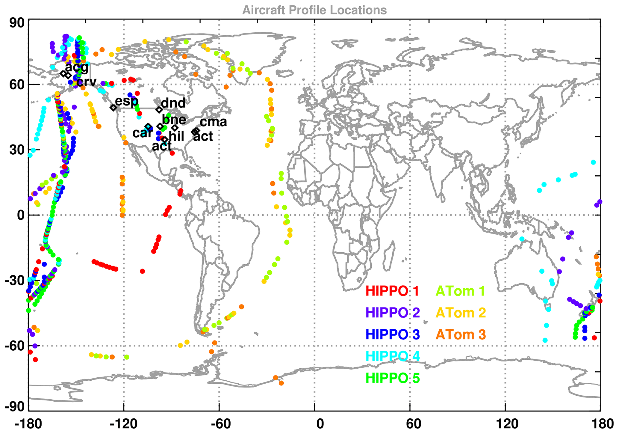
Figure 1 Locations of aircraft profiles used for HIPPO and ATom as colored dots and NOAA GML as black diamonds with a three-character string identifier. Most NOAA GML site codes represent the site name (e.g., “cma” stands for offshore Cape May, New Jersey), while some site codes such as “act” and “crv” represent NOAA GML profiles at various sites near the plotted code collected during campaigns.

Data from ATom aircraft campaigns 1–3 (Wofsy et al., 2018) are also used in this study: ATom-1, July–August 2016; ATom-2, January–February 2017; and ATom-3, September–October 2017. During Atom, the NASA DC-8 aircraft flew tracks with similar latitude coverage as HIPPO but also flew over both the Atlantic and Pacific oceans (Fig. 1). During flights, the aircraft continuously profiled the atmosphere from 0.2 to 12 km altitude with a similar average top to that of HIPPO. For this study, we use CO measurements on ATom from the QCLS instrument, similar to HIPPO, that are calibrated to the WMO X2014A scale (Novelli et al., 1991, 1994, 1998).

The NOAA GML observations are taken mainly at fixed sites in North America (Sweeney et al., 2015). In this study observations from the years 2006–2017 and from nine sites (Fig. 1) are used. The air samples are collected using an automated Programmable Flask Package (PFP) operated on small aircraft. Air samples are collected at several altitudes during a single flight, resulting in a vertical profile for each trace gas measured. The average top of the profiles in the data set used here was at 440 hPa. The CO mixing ratios are reported relative to the WMO X2014A CO scale. Uncertainties on the CO from the flasks are of the order of 1 ppb (Sweeney et al., 2015).

2.2 AIRS single-footprint CO retrievals

AIRS is a nadir-viewing, scanning thermal infrared (TIR) spectrometer launched on board the Aqua satellite on 4 May 2002 into a sun-synchronous polar orbit at an altitude of 705 km with 01:30 and 13:30 local Equator crossing times (Aumann et al., 2003). It measures the thermal radiance between 3 and 12 µm with a spectral resolution of ∼1.8 cm⁻¹ in the 4.6 µm (∼2100 cm⁻¹) CO absorption region. A single AIRS field of view (FOV) has a circular footprint with ∼15 km diameter at nadir, and the AIRS swath width is ∼1650 km, which enables near-global coverage twice daily.

Several algorithm evaluations have been published previously for retrievals of CO from AIRS, using Level 2 cloud-cleared radiances (Susskind et al., 2003) on the 45 km fields of regard (FORs), which encompass nine FOVs. These include the AIRS operational algorithm (first introduced by McMillan et al., 2005, with revisions through to the current v7), the NOAA Unique Combined Atmospheric Processing System (NUCAPS) (Gambacorta et al., 2015), the Community Long-term Infrared Microwave Combined Atmospheric Product System (CLIMCAPS) (Smith and Barnet, 2020), and the optimal estimation algorithm presented by Warner et al. (2010).

Here we present results of CO retrievals from AIRS radiances using the MUSES algorithm (Worden et al., 2006, 2013b; Fu et al., 2013, 2016, 2018, 2019; Kulawik et al., 2021). MUSES uses an optimal estimation approach (Rodgers, 2000) and leverages the algorithm developed for the Aura TES (Bowman et al., 2006). We use L1B radiances on single 15 km AIRS FOVs or footprints rather than cloud-cleared radiances on the 45 km FORs (comprised of nine FOVs) to preserve the original well-characterized radiance noise characteristics for use in our estimates (Irion et al., 2018; DeSouza-Machado et al., 2018). The Optimal Spectral Sampling (OSS) code was used as the forward model (Moncet et al., 2008, 2015). CO is retrieved using the 2181–2200 cm⁻¹ spectral range.

3 Validation methodology

3.1 Coincidence criteria and quality control

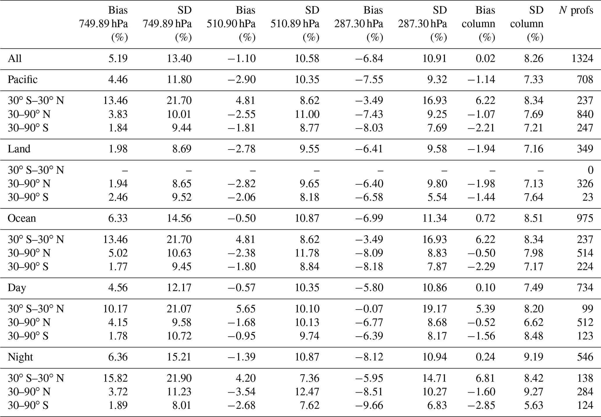
The AIRS and aircraft profiles were matched using time and distance coincidence criteria of 9 h and 50 km. The matched profiles were then subject to several quality control filters to form the final validation set. The aircraft profiles were required to have at least 10 pressure levels with valid CO data, and the difference between the maximum and minimum pressure of the valid data levels had to be at least 400 hPa. The AIRS MUSES algorithm provides a diagnostic retrieval quality flag, and this was used to remove poor or suspect retrievals from the set. While the AIRS MUSES algorithm uses the original single pixel instrument radiances rather than cloud-cleared radiances, the algorithm does retrieve cloud optical thickness following Kulawik et al. (2006) and provides both a spectrally varying and average effective optical depth. The cloud optical depth is retrieved before CO; thus, the effect of clouds is taken into account in the CO retrieval. AIRS MUSES profiles with optically thick clouds were designated as those with an average cloud effective optical depth over the AIRS spectrum and within the CO absorption band greater than 0.1 and were removed from the set. After the quality and cloud screening was applied, there remained 3734 AIRS–HIPPO matches representing 405 unique HIPPO aircraft profiles, 1324 AIRS–ATom matches representing 158 unique ATom aircraft profiles, and 10 044 AIRS–NOAA GML matches representing 747 unique NOAA GML aircraft profiles. Thus, each aircraft profile was compared to a set of AIRS profiles. All the aircraft profiles in the final data sets were interpolated vertically to the 67 AIRS MUSES forward-model levels.

3.2 Approach for error validation

Details of the retrieval error characterization from the optimal estimation (OE) approach of Rodgers (2000) and its application to instruments like AIRS are provided in many publications (e.g., Boxe et al., 2010; Oetjen et al., 2014; Kulawik et al., 2021). Here the details relevant to the error validation in this study are presented.

As described in Oetjen et al. (2014) the OE error covariance can be split up into several terms, as shown in Eq. (1), that represent the various factors contributing to the overall uncertainty S_z of a retrieved CO profile. These factors include smoothing due to limited vertical information content of the satellite instrument measurement (smoothing), instrument measurement noise (noise), uncertainties from parameters not included in the retrieval state vector (systematic), coupling interference or cross correlation between parameters retrieved simultaneously with CO (cross-state), and a residual term (res) that accounts for uncertainties not considered or unknown.

$$\begin{array}{}\text{(1)}& \begin{array}{rl}{\mathbf{S}}_z& =\underset{\text{smoothing}}{\left({\mathbf{A}}_{zz}-\mathbf{I}\right)}{\mathbf{S}}_{\mathrm{s}}{\left({\mathbf{A}}_{zz}-\mathbf{I}\right)}^T+\underset{\text{noise}}{{\mathbf{GS}}_e{\mathbf{G}}^T}\\ & +\underset{\text{systematic}}{\sum {\mathbf{GK}}_b{\mathbf{S}}_b}{\left({\mathbf{GK}}_b\right)}^T+\underset{\text{cross-state}}{\sum {\mathbf{A}}_{xs}{\mathbf{S}}_a^{b_{\mathrm{ret}}}}{\left({\mathbf{A}}_{xs}\right)}^T+\text{res}.\end{array}\end{array}$$

In the smoothing term I is the identity matrix, A_zz is the covariance matrix for CO, and S_s is the smoothing error covariance. In the noise term G is the gain matrix that describes the sensitivity of the retrieved state to changes in measured radiances and S_e is the instrument noise covariance. In the systematic term the subscript b represents parameters that are held constant during the retrieval with respective Jacobians, K_b, and error covariance matrix S_b. In the cross-state term the averaging kernels of the other parameters (x) retrieved simultaneously with CO are A_xs and the corresponding error covariance matrix is ${\mathbf{S}}_a^{b_{\mathrm{ret}}}$.

The averaging kernel matrix describes the vertical sensitivity of a retrieved parameter to its true state in the atmosphere. The vertical sensitivity is dependent on the true state vertical distribution of CO and other trace gases, retrieval constraints, and on the interference of other geophysical parameters such as the profiles of temperature and water vapor. The sum of the rows of the averaging kernel matrix provides information on the location of the peak sensitivity of the retrieval. Figure 2 shows the mean sum of the rows of the averaging kernel matrices for all the AIRS profiles in the validation set binned by latitude band: the level of peak sensitivity is generally between 400 and 500 hPa. The sensitivity peaks at a higher level in the tropical and sub-tropical latitude band of 30^∘ S–30^∘ N and at lower vertical levels in the higher latitude bands of both hemispheres.

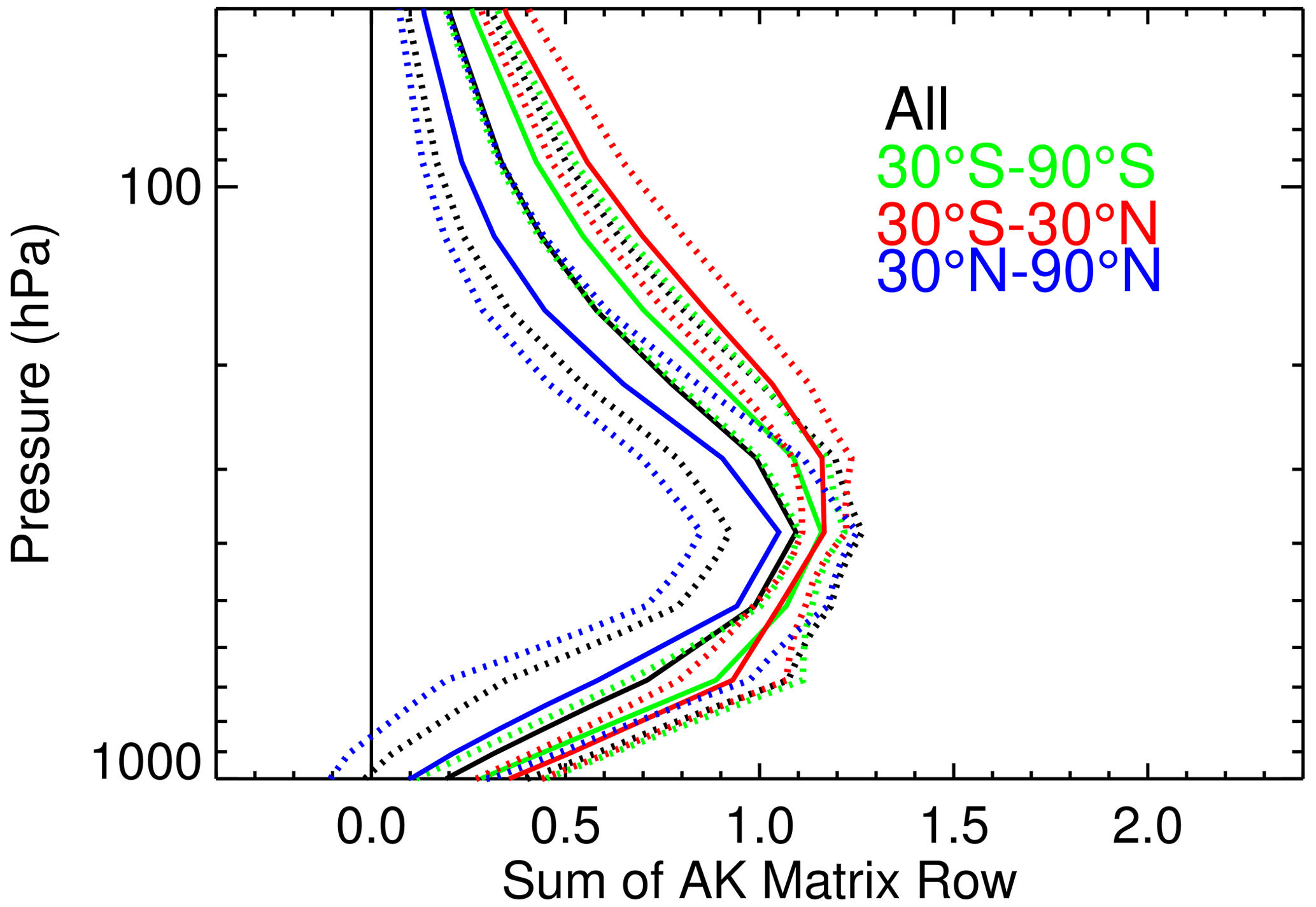
Figure 2 Mean (solid) sum of rows of the AIRS MUSES CO averaging kernels for each latitude band for the HIPPO retrievals. The dotted lines are 1 standard deviation from the mean. The peak of the mean generally corresponds to the vertical level of maximum AIRS sensitivity to the true state CO mixing ratio.

For comparing satellite profiles of trace gases with limited vertical resolution to profiles measured in situ from aircraft, the averaging kernel and an a priori profile is applied to the in situ profiles as in Rodgers and Connor (2003). Through this procedure a new profile $\widehat{\mathbf{Z}}$, representing what the satellite “sees” assuming no retrieval errors, is generated as shown in Eq. (2) from the averaging kernel A_zz applied to the difference between the elements of the original aircraft profile Z_aircraft and the a priori profile Z_apriori. For AIRS MUSES CO retrievals, the a priori profiles are obtained from a monthly climatology, in 30^∘ latitude by 60^∘ longitude boxes produced from the MOZART atmosphere chemistry model for the Aura mission (Brasseur et al., 1998). The a priori constraint used for CO is the same constraint used in the MOPITT CO algorithm (Deeter et al., 2010).

$$\begin{array}{}\text{(2)}& \widehat{\mathbf{Z}}={\mathbf{Z}}_{\mathrm{apriori}}+{\mathbf{A}}_{zz}({\mathbf{Z}}_{\mathrm{aircraft}}-{\mathbf{Z}}_{\mathrm{apriori}}).\end{array}$$

This procedure is also referred to as convolving the in situ profiles with the averaging kernel. Since there are no aircraft observations for the part of the retrieved profile above the aircraft flight levels, numerical techniques must be applied to extrapolate aircraft profiles above the flight levels (e.g., Kulawik et al., 2021); however, the uncertainty of the extrapolated measurements at these levels must be accounted for as it can propagate to the levels where there are actual aircraft observations through the application of the averaging kernel (Tang et al., 2020). For our study we simply fill the true aircraft profile above the aircraft flight levels with the a priori value. If the a priori value is representative of the average true atmosphere, this assumption should be reasonable. We explore the implications of this assumption using the NOAA GML set in Sect. 4.3.

The approach for error validation in this paper will start with a comparison of each AIRS-retrieved profile with the corresponding matched aircraft profile convolved with the averaging kernel; the results will be grouped in latitude bands ranging from the tropics to subpolar regions. Next, theoretical errors represented by all but the smoothing term of the error covariance of Eq. (1) will be evaluated for each retrieval, averaged within the latitude bands, and compared to the retrieval error standard deviation (uncertainty) and the a priori error. Finally, empirical errors calculated from an ensemble of retrieved profiles collocated with an aircraft profile as in Boxe et al. (2010) and Oetjen et al. (2014) will be evaluated for select CO plume and background cases. This approach will be applied separately to the HIPPO, ATom, and NOAA data sets, since each presented different characteristics.

4 Results

4.1 AIRS MUSES validation with HIPPO

The percent differences between AIRS MUSES and the HIPPO aircraft profiles are shown in Fig. 3. The profiles are plotted only up to 200 hPa, as there were few aircraft observations above that level, and are shown as the complete set and binned by latitude bands. For all groupings the mean biases are positive in the lower troposphere; tend toward zero in the middle troposphere, where the retrieval has greatest sensitivity; and become negative in the upper troposphere. The spread of the error profiles also tends to be narrower in the middle of the troposphere. Table 1 shows statistics corresponding to these plots and for the profiles grouped by land/ocean and day/night categories for selected pressure levels. The lowest biases are within plus or minus 3.1 % and occur at the 510 hPa level, while there are larger positive biases of 2 %–21 % at the 750 hPa level and negative biases up to ∼15 % at the 287 hPa level. There were no substantial or consistent differences for the error statics grouped by land vs. ocean and day vs. night, which suggests that these categories can be combined in the error analysis. Partial column average mixing ratios (referred to hereafter as column average mixing ratios) were calculated for each profile between the lowest to the highest aircraft flight level. The column average CO mixing ratios plotted by latitude (Fig. 4, top panel) show that the 30–90^∘ S band was predominantly in a background regime, with mixing ratios generally <70 ppbv, and that mixing ratios increased steadily with latitude to ∼150 ppbv by 30^∘ N. The average column CO mixing ratio bias (Fig. 4 bottom panel) also shows a latitude dependence with higher mean bias of ∼ 10–15 ppbv occurring near the 30^∘ N band. In addition, the error distribution is highly skewed toward positive numbers particularly in the 30–60^∘ N latitude band (skewness =1.36), indicating that the errors are not normally distributed.

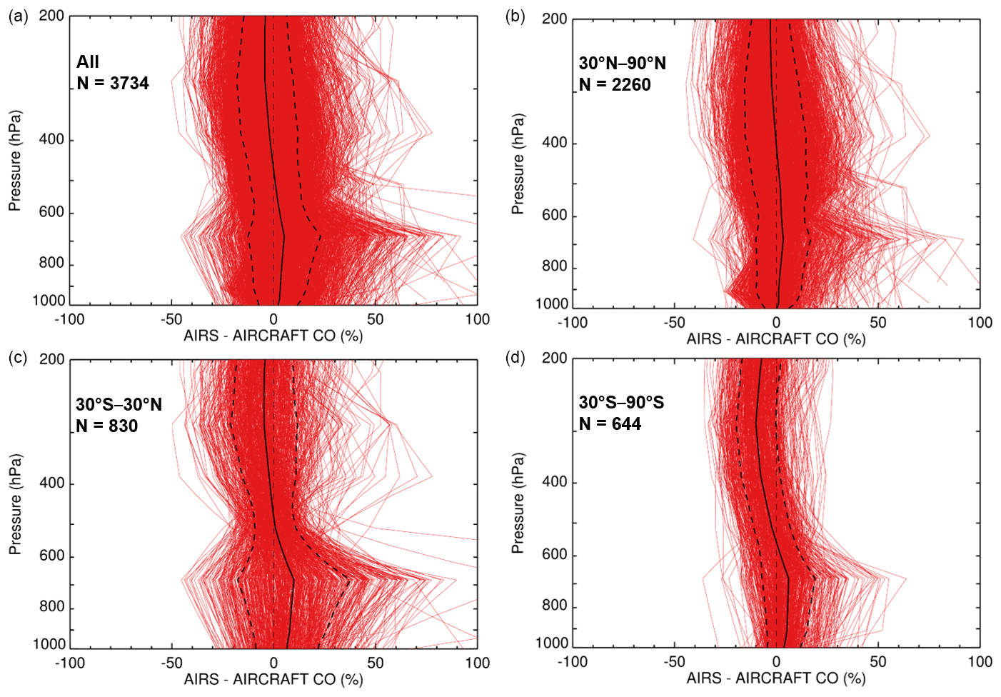
Figure 3 The AIRS MUSES–aircraft percent difference profiles for HIPPO. The number of profiles and the latitude bands are indicated in the upper left of each panel. All HIPPO profiles were convolved with the averaging kernels (Eq. 2) before the differences were calculated. The red lines indicate the individual profiles, the black solid lines the mean difference or bias, and the dashed lines 1 standard deviation from the mean.

Table 1 AIRS–aircraft CO statistics for HIPPO campaign.

Figure 4 The AIRS and HIPPO partial column average CO mixing ratios (a) and AIRS–HIPPO column average CO mixing ratio differences (b) by latitude. The column averages are calculated from the lowest to the highest flight altitudes for each profile. The black dots in panel (b) are the average differences within each 10^∘ latitude bin. The skewness of the error distribution is also shown. Skew values greater (less) than 1 indicate significant positive (negative) skew from a Gaussian distribution.

Beyond examining biases and variability of the retrieved profiles, evaluating the retrieval error estimates is also important, since they provide users with a measure of the reliability of the data. Following Oetjen et al. (2014) and Kulawik et al. (2021) we evaluated the AIRS MUSES retrievals by comparing the theoretical error estimates from the MUSES diagnostics to the actual retrieval error statistics described above. Figure 5 shows the profiles of the fractional estimated observation errors, mean a priori error, AIRS–aircraft standard deviation, and a priori–aircraft standard deviation. The errors are binned by latitude band, and the 30–90^∘ bands have been divided into two bands of 30–60 and 60–90^∘ in both hemispheres to better capture the dependence of error characteristics on latitude. The estimated observational error includes the noise, systematic, and cross-state error terms as shown in Eq. (1), and the mean a priori error is estimated from the square root of the diagonal of the a priori covariance matrix.

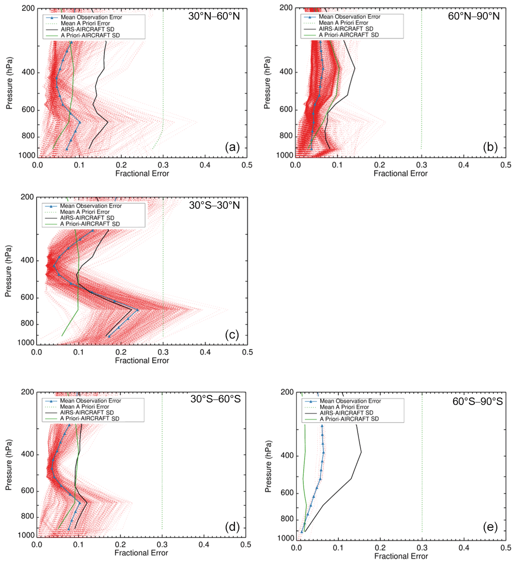
Figure 5 Estimated observational error analysis for the HIPPO data set. Estimated observation errors for each AIRS MUSES CO retrieval (dotted red lines), the mean observation error (solid blue line and triangles), the mean a priori error estimate (green line), and the standard deviation of the AIRS–HIPPO aircraft profiles differences and the standard deviation of the a priori–aircraft profile differences. The profiles are binned by latitudes bands 30–60^∘ N (a), 60–90^∘ N (b), 30^∘ S–30^∘ N (c), 30–60^∘ S (d), and 60–90^∘ S (e).

The estimated observational errors (red lines are individual errors, and the blue lines are the mean) are lowest around 500 hPa, where AIRS sensitivity is greatest, and this pattern is similar to the actual error profiles shown in Fig. 3. The minimum error shifts downwards towards the poles, with the smallest errors occurring lower at about 650 hPa in the Arctic region 60–90^∘ N; however, in the Antarctic region (60–90^∘ S) there were not enough AIRS–aircraft profile matches where the AIRS profiles passed quality screening to provide a reasonable set of statistics.

The standard deviation for the a priori–aircraft differences (green) is lower than the standard deviation for the AIRS–aircraft differences (black); for this data set the a priori profiles appear to be a better estimate of the true profiles than the retrievals; however, the skewness of the column mixing ratio differences suggests that Gaussian statistics do not provide an accurate representation of the error characteristics of this data set; i.e., a simple average of error estimates is not very meaningful. Note also the average estimated error (blue) is significantly lower than the AIRS–aircraft differences (black) except below 600 hPa in the 30^∘ S–60^∘ N band, which is also likely due to the skewness of the data differences.

An alternative approach for evaluating the theoretical error is to compare it to the variability within the set of AIRS profiles collocated with an aircraft profile. If it is assumed that all satellite footprints in the collocated set are basically seeing the same scene, then the variability in the retrieved profiles can be considered an empirical error (Oetjen et al., 2014). In this analysis the empirical error is referred to simply as the AIRS profile variability. Using this approach, plume and background cases were selected for each of the five HIPPO missions. The case profiles were chosen using the maximum and minimum CO mixing ratios for each campaign at the 464.16 hPa pressure level of the remapped aircraft profiles. In addition to the CO mixing ratio criteria a minimum of eight co-located AIRS profiles that met the quality control standards had to be available for the case to be selected. A mean observation error for this set of co-located AIRS profiles is calculated like that in Fig. 5. The AIRS profile variability was estimated as the square root of the diagonal of the covariance matrix of all the coincident AIRS MUSES retrievals. In general, for these cases, the AIRS profile variability was of the same magnitude as the mean observation error, and the absolute differences was less than 10 %. For the background cases the AIRS profile variability is generally comparable to the mean observation error. For the plume cases, we might expect to see larger discrepancies between the mean observation error and the AIRS profile variability due to actual atmospheric variability in the region of the plume.

Illustrative cases for HIPPO-2 and HIPPO-3 are presented in Fig. 6. The plume case for HIPPO-2 is in the Arctic; the aircraft data feature a very high spike (∼270 ppbv) near 400 hPa that the mean AIRS profile does not capture (Fig. 6 bottom left panel). The AIRS profile variability has a large peak >15 % at about the same level that is much larger than the mean observation error (Fig. 6 top left panel). For the HIPPO-3 plume case the observed CO is also high, with peaks greater than 200 ppb in the middle troposphere. In this case, the AIRS mean retrieval does capture a peak (Fig. 6 right bottom panel), and the AIRS profile variability and mean observation error are in reasonable agreement.

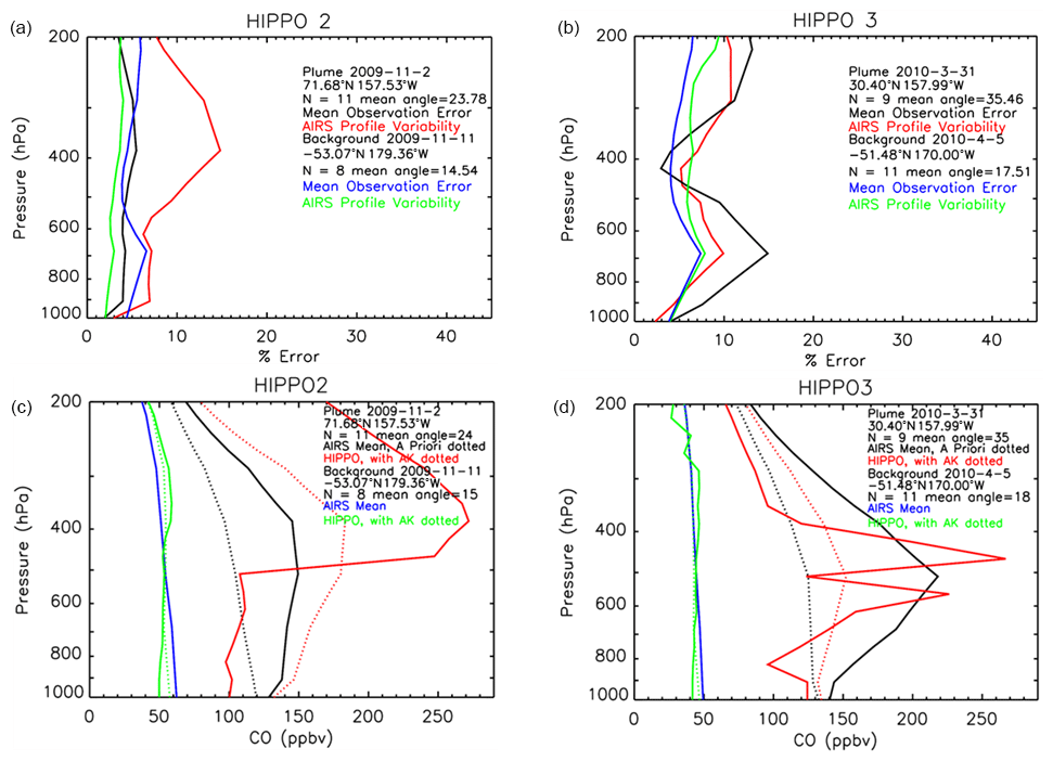
Figure 6 Mean observation error and AIRS profile variability for selected plume and background cases from the HIPPO campaign (a, b). Mean observation errors are black (plume profiles) and blue (background profiles), and AIRS profile variabilities are red (plume profiles) and green (background profiles). In panels (c) and (d) the plume (red) and background (green) HIPPO and average AIRS profiles (plume black, background blue) corresponding to the mean observation error and AIRS profile variability profiles in panels (a) and (b) are shown. The HIPPO profiles are shown without (solid) and with (dotted) the application of the AIRS averaging kernel. The average AIRS a priori profiles are shown for the plume cases only as black dots.

4.2 AIRS MUSES validation with ATom

The same steps were followed for the analysis of the ATom data set. The percent differences between AIRS MUSES and the ATom aircraft profiles are shown in Fig. 7 for different latitude bands, and the error statistics corresponding to these plots are shown in Table 2. As with HIPPO the smallest biases are in the middle troposphere and cover a similar range (from $\sim -\mathrm{4}$ % to +5 % vs. −3 % to +3 %). Like HIPPO, the average column mixing ratios (Fig. 8) show the same general dependence on latitude, as do the column errors. However, for HIPPO the aircraft column average CO mixing ratios in the 30^∘ S–10^∘ N band were all less than 100 ppbv (Fig. 4 top), whereas for ATom they were much more variable and were as high as ∼130 ppbv (Fig. 8 top). For 30–40^∘ N the HIPPO column mixing ratios ranged from ∼70 to ∼140 ppbv, whereas for ATom they were lower, ranging from ∼60 to ∼125 ppbv. These differences in air mass CO were associated with ATom errors that were positive in the 30^∘ S–10^∘ N band and negative around 30^∘ N (Fig. 8 bottom), and the opposite sign errors were in the corresponding latitude bands for HIPPO. The estimated observational errors for ATom (Fig. 9) were smallest in the middle troposphere, like HIPPO. However, the standard deviation of the AIRS–aircraft differences is smaller for the ATom comparisons than for the HIPPO comparisons. In the vertical range where AIRS has good sensitivity to CO (∼ 600–200 hPa), the standard deviation of the AIRS–ATom differences is generally less than the standard deviation of the a priori–ATom differences, except south of 30^∘ S, where there are mostly low levels of CO. The distribution of errors for 30–60^∘ N is less skewed than for HIPPO (0.54 vs. 1.36), suggesting that a Gaussian distribution of errors is a reasonable assumption for this data set. The difference between HIPPO and ATom was most evident in the 30–60^∘ N band where for HIPPO the retrieval error standard deviation was ∼4 % larger than the a priori error standard deviation (Fig. 6), whereas for ATom the retrieval error standard deviation was ∼5 % smaller than the a priori error standard deviation.

Figure 7 The AIRS MUSES–aircraft percent difference profiles for ATom campaigns 1–3. The number of profiles and the latitude bands are indicated in the upper left. All ATom profiles were convolved with the averaging kernels (Eq. 2) before the differences were calculated. The red lines indicate the individual profiles, the black solid lines the mean difference or bias, and the dashed lines 1 standard deviation from the mean.

Table 2 AIRS–aircraft CO statistics for ATom campaigns 1–3.

NA: not available.

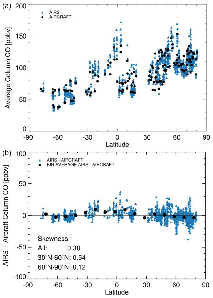
Figure 8 The AIRS and ATom partial column average CO mixing ratios (a, b) and AIRS–ATom column average CO mixing ratio differences (c, d) by latitude. The column averages are calculated from the lowest to the highest flight altitudes for each profile. The black dots in the bottom figure are the average differences within each 10^∘ latitude bin.

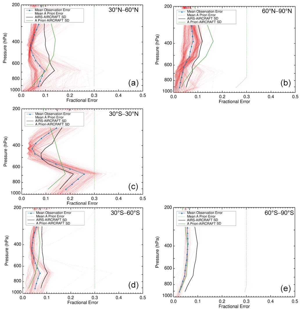
Figure 9 Estimated observational error analysis for the ATom data set. Estimated observation errors for each AIRS MUSES CO retrieval (dotted red lines), the mean observation error (solid blue line and triangles), the mean a priori error estimate (green line), and the standard deviation of the AIRS MUSES–ATom aircraft profiles differences and the standard deviation of the a priori–aircraft profile differences. The profiles are binned by latitudes bands 30–60^∘ N (a), 60–90^∘ N (b), 30^∘ S–30^∘ N (c), 30–60^∘ S (d), and 60–90^∘ S (e).

The reason for the better retrieval performance relative to the prior for the ATom vs. the HIPPO comparisons is not immediately clear. For the 30–60^∘ N latitude band, the mean and standard deviation of the average column CO amounts for HIPPO and ATom were similar at 103 and 108 ppbv and 409 and 445 ppb respectively. The data sets have similar seasonal coverage. There was a significant difference in geographic coverage: the HIPPO flights only covered the Pacific Ocean and adjacent land, whereas ATom additionally flew over the Atlantic Ocean (Fig. 1). To determine if this difference influenced the statistics a subset of the ATom data set was generated that considers only points west of 75^∘ W longitude. The statistics for this case are shown in Table 2 in the row labeled “Pacific”. While the bias at 510 hPa is slightly more negative for the Pacific case at −2.98 % compared to −1.10 % for all cases, the standard deviation of the AIRS–aircraft differences is similar. Furthermore, for the Pacific case there was no significant skew in the column average mixing ratio error distribution (30–60^∘ N skewness =0.29), and the estimated observation error profiles (not shown) were similar to those in Fig. 9. Therefore, it does not appear that the different geographic coverage between HIPPO and ATom was the cause of the differences in the error statistics.

Figure 10 shows example comparisons of mean observation error and AIRS profile variability estimates for selected AIRS–ATom matches (as presented for HIPPO in Fig. 6). The plume in the ATom-1 example is retrieved at a much higher altitude than observed, and the AIRS profile variability is much greater than the mean observation error (Fig. 10 left panels), while in the ATom-2 example there is a better agreement between the retrieved and observed profiles, and the AIRS profile variability and mean observation error are comparable. Overall, this analysis shows similar features to the analysis of estimated observation errors by latitude band in Fig. 9.

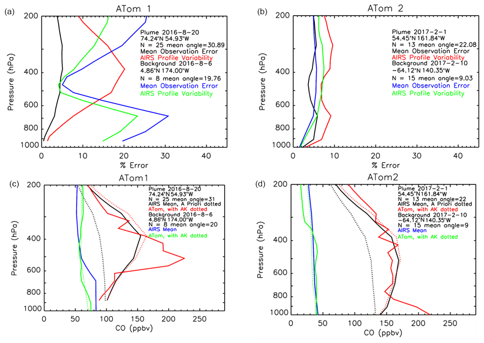
Figure 10 Mean observation error and AIRS profile variability for selected plume and background cases from the ATom campaigns (a, b). Mean observation errors are black (plume profiles) and blue (background profiles), and AIRS profile variabilities are red (plume profiles) and green (background profiles). In panels (c) and (d) the plume (red) and background (green) ATom and average AIRS profiles (plume black, background blue) corresponding to the mean observation error and AIRS profile variability in (a) and (b) are shown. The ATom profiles are shown without (solid) and with (dotted) the application of the AIRS averaging kernel. The average AIRS a priori profiles for the plume cases only are shown as black dots.

4.3 AIRS MUSES validation with NOAA GML

The NOAA GML data set was much larger, spanning a much longer period (2006–2017), but provided results over only a limited number of locations in North America (Fig. 1). For the NOAA GML set the AIRS MUSES retrieval error profiles are shown in Fig. 11 and statistics are shown in Table 3. Table 3 indicates that there are about a third of the matched profiles listed as ocean points, which seems to contradict the map in Fig. 1 that shows all the NOAA GML locations over land. However, the land/ocean classification is based on the MUSES land/ocean flag, and several of the NOAA GML locations are at the coast and one, “cma”, is identified as offshore Cape May. Therefore, a substantial number of the AIRS FOVs within the 50 km radius of the NOAA GML profiles near the coast and those corresponding to “cma” were classed as ocean.

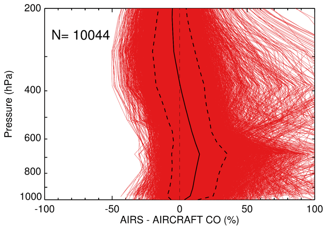
Figure 11 The AIRS MUSES–aircraft percent difference profiles for NOAA GML aircraft observations. All aircraft profiles were convolved with the averaging kernels (Eq. 2) before the differences were calculated. The red lines indicate the individual profiles, the black solid lines the mean difference or bias, and the dashed lines 1 standard deviation from the mean.

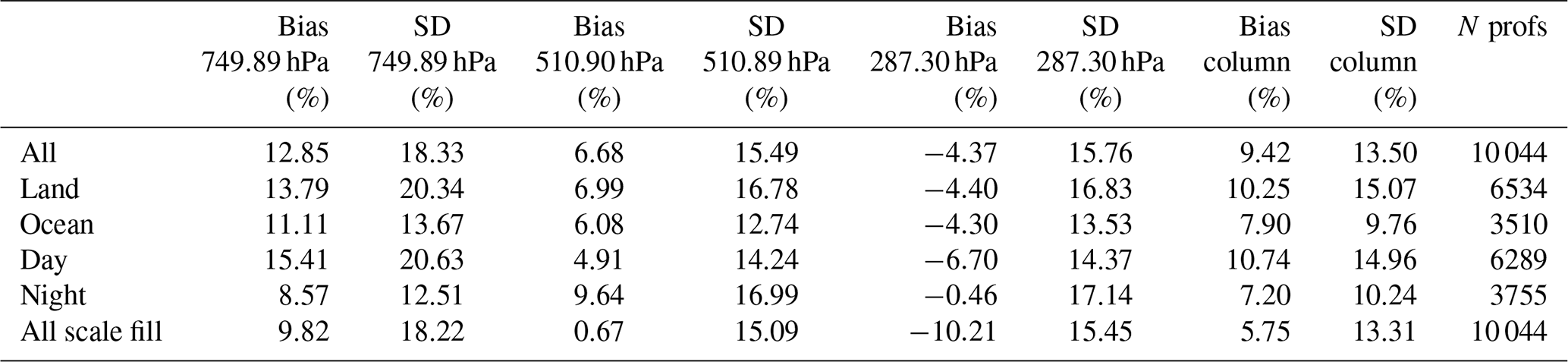
Table 3 AIRS–aircraft CO statistics for the NOAA GML observations. By default, the aircraft profiles are filled above the flight levels with the a priori profile. Additional statistics are generated by filling above the flight level with the a priori scaled by the difference between the a priori and the aircraft value at the highest flight level (All scale fill).

The column average mixing ratio errors by latitude are shown in Fig. 12. Overall, the retrievals have a noticeably larger positive bias in the lower troposphere compared to the HIPPO and ATom sets.

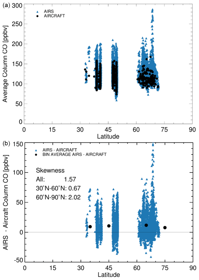
Figure 12 The AIRS and NOAA GML partial column average CO mixing ratios (a) and AIRS–NOAA GML aircraft column average CO mixing ratio differences (b) by latitude. The column averages are calculated from the lowest to the highest flight altitudes for each profile. The black dots in the bottom figure are the average differences within each 10^∘ latitude bin.

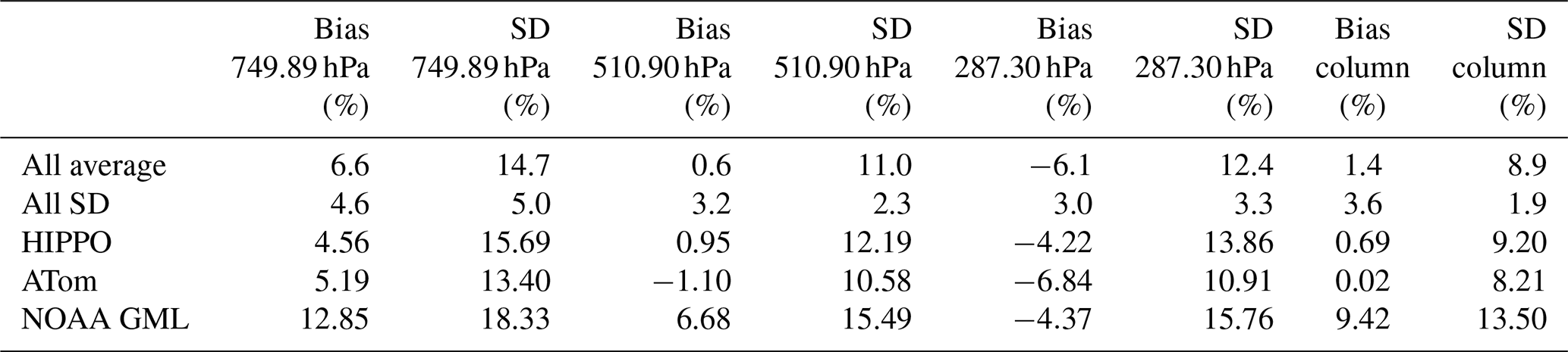
At the 510 hPa level the biases over land/ocean and day/night categories range from 4.9 %–9.6 % for the NOAA GML set (Table 3) compared to less than plus or minus 4 % for the HIPPO and ATom sets in the corresponding 30–90^∘ N latitude band (Tables 1 and 2). The column average mixing ratios are also biased much higher, ranging from 7.2 %–10.7 % for NOAA GML (Table 3) compared to within plus or minus 2 % for the HIPPO and ATom sets (Tables 1 and 2). The higher biases seem consistent across the latitudinal range of the NOAA GML observations as shown in Fig. 12. The theoretical observations errors for the NOAA GML set (Fig. 13) are similar to those of the HIPPO set (Fig. 5) with larger AIRS MUSES–aircraft error standard deviations than the mean observation errors and the a priori error standard deviations. As with HIPPO the column average mixing ratio errors are highly skewed toward positive values with an overall skewness of 1.57. This suggests that the assumption of a Gaussian error distribution upon which the observational error analysis is based is also not valid for the NOAA GML set.

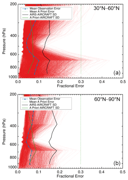
Figure 13 Estimated observational error analysis for the NOAA GML data set. Estimated observation errors for each AIRS MUSES CO retrieval (dotted red lines), the mean observation error (solid blue line and triangles), the mean a priori error estimate (green line), and the standard deviation of the AIRS MUSES–NOAA GML aircraft profiles differences and the standard deviation of the a priori–aircraft profile differences. The profiles are binned by latitudes bands 30–60 (a) and 60–90^∘ N (b).

We hypothesized that the higher retrieval biases for the NOAA GML set may be an artifact of larger errors associated with extrapolation of the aircraft profiles above the uppermost measurement altitude. The NOAA GML profiles have an average highest flight level near 440 hPa compared to 290 hPa for the HIPPO and ATom sets, and therefore there are more retrieval levels to fill in the remapped aircraft profile. These extra fill levels can cause greater error uncertainty in the lower levels when the averaging kernel matrix is applied. Tang et al. (2020) found that errors in MOPITT aircraft CO comparisons were very sensitive in the middle and upper troposphere to the method used to extend the aircraft profile.

To test the sensitivity of the AIRS retrieval statistics to the mixing ratio values used to fill the aircraft profiles, an additional set of statistics was generated using a scaled a priori value to fill the aircraft profiles above the flight levels. The scaled a priori value used a constant scale ratio between the mixing ratio at the highest aircraft level and the a priori at that level. The retrieval statistics for this experiment are shown in the last row of Table 3. For the scaled a priori fill case the bias at 510 hPa is only 0.7 % but the column average mixing ratio bias is still large at 5.8 %. Clearly the choice of fill value has a large impact on the retrieval error statistics.

The 12 years of NOAA GML CO profiles 2006–2017 provided the opportunity to investigate the retrieval performance over time as shown in the AIRS and aircraft time series plot of Fig. 14. There is a distinct seasonal cycle in the NOAA GML observations with high values occurring during the Northern Hemisphere winter and lower values in the summer, which is also captured by the AIRS retrievals. The bias drifts over this period (Fig. 15) are small, <0.5 % yr⁻¹ in magnitude, for all levels and the column average. They are also of approximately the same magnitude as those reported by Deeter et al. (2019) for MOPITT. There is a distinctive seasonal cycle to the bias errors in middle and lower troposphere and column averages with biases as high as 20 % in the summer months and biases approaching zero during the winter months. We hypothesize that this pattern is a result of greater photolytic destruction of the CO in the summer months leading to lower background values not always captured by the retrieval perhaps due to average a priori profiles being too high. We also examined the relationship between retrieval bias and the CO mixing ratio (Fig. 16). The bias sensitivity is greater in the lower troposphere with average biases at the 749 hPa pressure level ranging from positive 20 % at low CO mixing ratios to near zero at higher mixing ratios with an average slope of −0.16 % ppbv⁻¹. At the 510 hPa pressure level and for the column averages there is no marked dependence.

Figure 14 AIRS MUSES CO retrieval (red) and corresponding NOAA GML observations (blue) for select pressure levels and the aircraft column averages.

Figure 15 AIRS MUSES CO retrieval relative bias (%) drift for select pressure levels and the aircraft column averages for the NOAA GML observations.

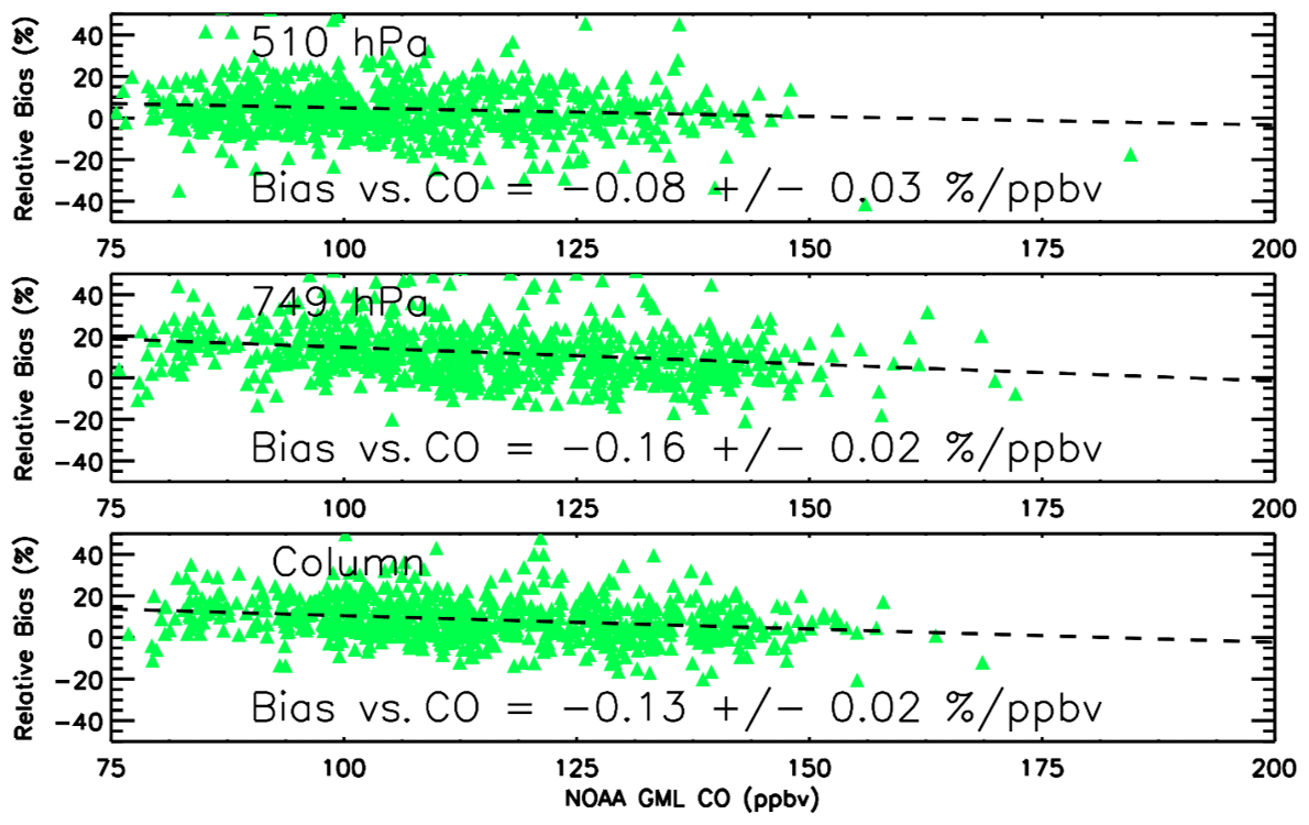
Figure 16 AIRS MUSES CO retrieval relative bias (%) versus CO for select pressure levels and the aircraft column averages for the NOAA GML observations.

5 Discussion and conclusions

A total of 15 112 quality-controlled AIRS single-footprint CO retrievals were evaluated with a total of 1310 aircraft profiles from the HIPPO and ATom aircraft campaigns and the ongoing NOAA GML measurement program. Single-footprint retrievals provide better spatial resolution over the AIRS operational CO product that uses a 3×3 footprint array of cloud-cleared radiances. The enhanced resolution should enable plumes from local anthropogenic sources and small fires to be better resolved and tracked. This evaluation seeks to quantify the error uncertainty in this new product to provide end users a measure of its reliability.

The AIRS CO retrievals were produced using the MUSES optimal estimation algorithm that utilizes techniques first applied to the Aura TES instrument. The AIRS profiles were matched with aircraft profiles with space and time coincidence criteria of 50 km and 9 h. The aircraft profiles of CO mixing ratio were first convolved with the AIRS averaging kernel to account for AIRS vertical sensitivity and then compared with the retrieved profiles. In addition, partial column average CO mixing ratios (referred to as column average mixing ratios for simplicity) defined as those between the highest and lowest aircraft flight level for each profile were estimated and compared to the corresponding AIRS values.

Table 4 Summary AIRS–aircraft CO statistics for all aircraft campaigns and categorizations.

The averaging kernels generated by the MUSES algorithm indicated that the level of greatest AIRS sensitivity to CO was in the middle troposphere at or near the 510 hPa retrieval level. The estimated observation error also showed the lowest values at this level. Overall mean biases were $+\mathrm{6.6}\pm \mathrm{4.6}$ %, $+\mathrm{0.6}\pm \mathrm{3.2}$ %, $-\mathrm{6.1}\pm \mathrm{3.0}$ %, and 1.4±3.6 % for 750, 510, 287 hPa, and the full column, respectively (Table 4). The mean standard deviations were 15 %, 11 %, 12 %, and 9 % at these same pressure levels, respectively. For the HIPPO and ATom profile sets, the overall biases at the 510 hPa level were 0.95 % and −1.10 % respectively. For both HIPPO and ATom, the AIRS CO comparison statistics had little sensitivity to land/ocean or day/night categorization. Column average mixing ratios by latitude for both sets exhibited lower mixing ratios in the 30–90^∘ S band of about 50–70 ppbv, with increasing values toward the north reaching ∼ 125–150 ppbv at 30^∘ N. While the column average errors were similar in both sets, the errors were highly skewed in the positive for HIPPO particularly in the 30–60^∘ N latitude bands. Estimated observation errors from the AIRS MUSES algorithm were generally small as expected in the middle troposphere where AIRS has good sensitivity. However, for HIPPO in the 30–60^∘ N band the retrieval error standard deviation was ∼4 % higher than expected, possibly because the algorithm assumes a Gaussian error distribution and the errors were highly positively skewed in that region. The AIRS retrievals were able to distinguish between plume and background cases in the HIPPO case but were not always able to capture sharp vertical gradients or pinpoint the vertical location of the plume feature.

The retrieval errors for the NOAA GML profiles were considerably higher than those for the HIPPO and ATom sets. The 510 hPa and column average biases were 6.7 % and 9.4 % respectively. Like HIPPO, the column average errors were highly skewed in the positive, suggesting a non-Gaussian distribution of errors and possibly explaining the much higher error standard deviation than the estimated theoretical observation error. The statistics of AIRS–aircraft differences were shown to be very sensitive to the values used to fill the aircraft profiles above the flight level due to the propagation of error uncertainty to lower retrieval levels through the averaging kernel convolution procedure. Using a scaled a priori profile for the fill value resulted in a considerably smaller bias at the 510 hPa level of 0.7 % and a slightly smaller column average bias of 5.8 %.

The results of the NOAA GML comparisons were more strongly affected by the choice of fill value above the flight level than the HIPPO or ATom comparisons since the NOAA GML profiles had a lower top with an average of 440 hPa compared to HIPPO and ATom with an average top at 290 hPa.

The 12 years of NOAA GML CO profiles 2006–2017 provided the opportunity to evaluate the AIRS MUSES retrieval performance over time. The AIRS MUSES retrievals mostly capture the distinct observed seasonal cycle that featured higher mixing ratios in the winter and lower mixing ratios in the summer. However, the AIRS CO mixing ratios seemed to be biased high by ∼20 % in the summer in the lower troposphere. The bias drift for 2006 to 2017 was also evaluated using the NOAA GML set and shown to be small (<0.5 % yr⁻¹).

Overall, these validation results show no appreciable latitudinal dependence in the bias and that the bias drift over time is small. This suggests that the retrieval data can be used reliably to compare regional differences in CO mixing ratios and to track trends over time. Furthermore, the higher spatial resolution compared to the operational product should enable better detection and tracking of small plumes and more robust trend analysis of the higher end mixing ratios that are likely to be muted due to smoothing in the coarser product. An important finding for future algorithm development was that the algorithm-diagnosed observation errors were underestimating the actual retrieval errors. The cause of this underestimation requires further investigation.