the Creative Commons Attribution 4.0 License.
the Creative Commons Attribution 4.0 License.
 | 03 Jan 2022
Towards operational multi-GNSS tropospheric products at GFZ Potsdam
Galina Dick
Florian Zus
Jens Wickert
The assimilation of global navigation satellite system (GNSS) data has been proven to have a positive impact on weather forecasts. However, the impact is limited due to the fact that solely the zenith total delays (ZTDs) or integrated water vapor (IWV) derived from the GPS satellite constellation are utilized. Assimilation of more advanced products, such as slant total delays (STDs), from several satellite systems may lead to improved forecasts. This study shows a preparation step for the assimilation, i.e., the analysis of the multi-GNSS tropospheric advanced parameters: ZTDs, tropospheric gradients and STDs. Three solutions are taken into consideration: GPS-only, GPS–GLONASS (GR) and GPS–GLONASS–Galileo (GRE). The GNSS estimates are calculated using the operational EPOS.P8 software developed at GFZ. The ZTDs retrieved with this software are currently being operationally assimilated by weather services, while the STDs and tropospheric gradients are being tested for this purpose. The obtained parameters are compared with the European Centre for Medium-Range Weather Forecasts (ECMWF) ERA5 reanalysis. The results show that all three GNSS solutions show similar level of agreement with the ERA5 model. For ZTDs, the agreement with ERA5 results in biases of approx. 2 mm and standard deviations (SDs) of 8.5 mm. The statistics are slightly better for the GRE solution compared to the other solutions. For tropospheric gradients, the biases are negligible, and SDs are equal to approx. 0.4 mm. The statistics are almost identical for all three GNSS solutions. For STDs, the agreement from all three solutions is very similar; however it is slightly better for GPS only. The average bias with respect to ERA5 equals approx. 4 mm, with SDs of approx. 26 mm. The biases are only slightly reduced for the Galileo-only estimates from the GRE solution. This study shows that all systems provide data of comparable quality. However, the advantage of combining several GNSS systems in the operational data assimilation is the geometry improvement by adding more observations, especially for low elevation and azimuth angles.
- Article
(9226 KB) - Full-text XML
- BibTeX
- EndNote


During the past decades, the number of heavy rainfall, flash floods and other severe weather events has been increasing. One way to improve the forecasts of such phenomena is to assimilate more meteorological observation data into the numerical weather models (NWMs) (Poli et al., 2007; Zus et al., 2011; Bennitt and Jupp, 2012; Rohm et al., 2019). In addition to the typical data sources for the assimilation such as radiosonde profiles, satellite and ground-based meteorological observations or aviation data, global navigation satellite system (GNSS) data can also provide valuable information. Studies show that the assimilation of the GNSS zenith total delays (ZTDs) or integrated water vapor (IWV) can have a positive impact on the weather forecasts. Case-based studies show an increase of the quality of the humidity and precipitation forecasts (Cucurull et al., 2007; Boniface et al., 2009; Kawabata et al., 2013; Saito et al., 2017; Rohm et al., 2019). Nowcasting studies also show an improvement in forecasts, especially for water vapor while using the GNSS estimates (Smith et al., 2000; Benevides et al., 2015; Benjamin et al., 2016).
Some meteorological agencies such as the UK Met Office, German Weather Service (DWD) or Japan Meteorological Agency (JMA) are operationally assimilating the GNSS tropospheric products. The challenge in the operational assimilation of the GNSS data is that the weather systems are already assimilating many observations from other data sources. Thus, in the related assimilation studies, the impact of GNSS data is reported just as slightly positive or neutral (Poli et al., 2007; Bennitt and Jupp, 2012; Lindskog et al., 2017). Moreover, these studies are only focused on the use of tropospheric parameters in the zenith direction, i.e., ZTD or IWV. More advanced products, such as tropospheric gradients or slant total delays (STDs), are of interest, since information on the horizontal distribution is provided by these parameters. A positive impact of the STD assimilation on forecasts is to be expected, as it provides tropospheric information in many different directions. The first assimilation experiments using tropospheric gradients were undertaken by Zus et al. (2019).
This study is conducted within the recent research project Advanced MUlti-GNSS Array for Monitoring Severe Weather Events (AMUSE) of the German Research Foundation (DFG). The main objectives of this project are (1) developments to provide high-quality slant tropospheric delays instead of only zenith delays, (2) developments to provide multi-GNSS products instead of GPS-only, (3) developments to provide ultra-rapid tropospheric information and (4) monitoring and assimilation of the tropospheric products. Here, we focus on the two first objectives. We show the comparisons of multi-GNSS tropospheric products, obtained using three satellite systems: the US American Global Navigation System (GPS), Russian GLONASS and European Galileo. We calculate the tropospheric parameters from three systems for the stations located worldwide, with special emphasis on Germany using the in-house-developed software Earth Parameter and Orbit determination System (EPOS.P8). We compare our estimates with the European Centre for Medium-Range Weather Forecasts (ECMWF) ERA5 reanalysis. The outcomes of this study will be assimilated in an operational manner by the DWD. This study is thus a preparation step for the assimilation that shows the tropospheric parameters from the operational software EPOS.P8 developed and run at GFZ. Moreover, the GFZ is one of the analysis centers for the EUMETNET EIG GNSS Water Vapour Programme (E-GVAP; http://egvap.dmi.dk/, last access: 17 December 2021) and, as such, provides the ZTD and in the future STD estimates to the weather agencies for the assimilation.
Many previous studies compared the tropospheric parameters from GNSS and NWM data for ZTD or IWV (Vedel et al., 2001; Teke et al., 2011; Wilgan et al., 2015; Douša et al., 2016; Hadaś et al., 2020; Lu et al., 2020; Bosser and Bock, 2021), the tropospheric gradients (Li et al., 2015b; Lu et al., 2016; Douša et al., 2017; Elgered et al., 2019; Kačmařík et al., 2019) or STD (de Haan et al., 2002; Bender et al., 2008; Li et al., 2015a; Kačmařík et al., 2017). However, the majority of these studies are focused on the comparisons in the zenith direction, and the estimates were calculated from the GPS-only data, sometimes GPS–GLONASS combination. This study shows a comprehensive comparison of all three tropospheric parameters, i.e., ZTDs, tropospheric gradients and STDs, with a main focus on the multi-GNSS estimates. It is also one of the first works showing all three tropospheric parameters from multi-GNSS solution with fully operational Galileo constellation. A detailed comparison with some selected studies covering similar aspects is shown in Sect. 5 – Discussion.
This Introduction is followed by Sect. 2 explaining the tropospheric parameters. Section 3 describes the GNSS and NWM data. Section 4 shows the comparison of three different tropospheric parameters, Sect. 5 discusses our findings in view of the previous studies and the results are summarized in Sect. 6.
The microwave signals propagating through the atmosphere are delayed in its lowest part, the neutral atmosphere, which consists of the troposphere, stratosphere and a part of the mesosphere (and is here called “troposphere” for shortness). The delay is caused by the propagation medium, which is characterized by meteorological parameters: temperature, air pressure and water vapor. The impact can be expressed by the refraction index n. Since this index is very close to unity, usually a parameter called total refractivity N is used (Essen and Froome, 1951):
The total refractivity can be calculated from the meteorological parameters using the following equation (Thayer, 1974):
where p is the atmospheric air pressure (hPa); e is the water vapor partial pressure (hPa); T is the temperature (K), k1=77.60 (K hPa−1), k2=70.4 (K hPa−1) and k3=373 900 (K hPa−2) are the refractivity coefficients, here taken from Bevis et al. (1994); and and are the inverse compressibility factors for dry air and water vapor, respectively, usually assumed to be 1.
From the total refractivity, a tropospheric delay in either the zenith (ZTD) or slant direction (STD) can be calculated:
where Δ denotes the delay, S denotes the arc-length of the ray path and g denotes the geometric distance between the station and the satellite. In the GNSS analysis, the slant tropospheric delay is approximated according to
where ZHD and ZWD are the hydrostatic and wet parts of the ZTD, respectively; GN and GE denote the north–south and east–west gradient components; MFh, MFw and MFg are the mapping functions for the hydrostatic, wet part (e.g., Böhm et al., 2006) and gradients (e.g., Bar-Sever et al., 1998; Chen and Herring, 1997), respectively; el is the elevation angle; A the azimuth angle; and res is the post-fit phase residuals.
We have processed the initial data from three multi-GNSS solutions and ERA5 for the entire year of 2020. In this section, we describe the data sources in more detail.
3.1 GNSS data
Our study incorporates GNSS data from three systems: GPS (G), GLONASS (R) and Galileo (E) for 663 stations worldwide from the German national network SAPOS, the International GNSS Service (IGS; http://www.igs.org, last access: 17 December 2021, Johnston et al., 2017) network, the EUREF Permanent Network (EPN; http://www.epncb.oma.be, last access: 17 December 2021) and the GFZ network (Ramatschi et al., 2019). Unfortunately, not all used stations are adapted to receive all types of GNSS signals yet. The number of stations capable of receiving particular signals for the whole world and specifically for Germany is given in Table 1. Figure 1 shows the map of all stations for the whole world and Fig. 2 for Germany. For most of our comparisons (for ZTDs and tropospheric gradients), we consider only the GRE-capable stations.
Table 1Number of stations capable of receiving particular GNSS signals used in this study.
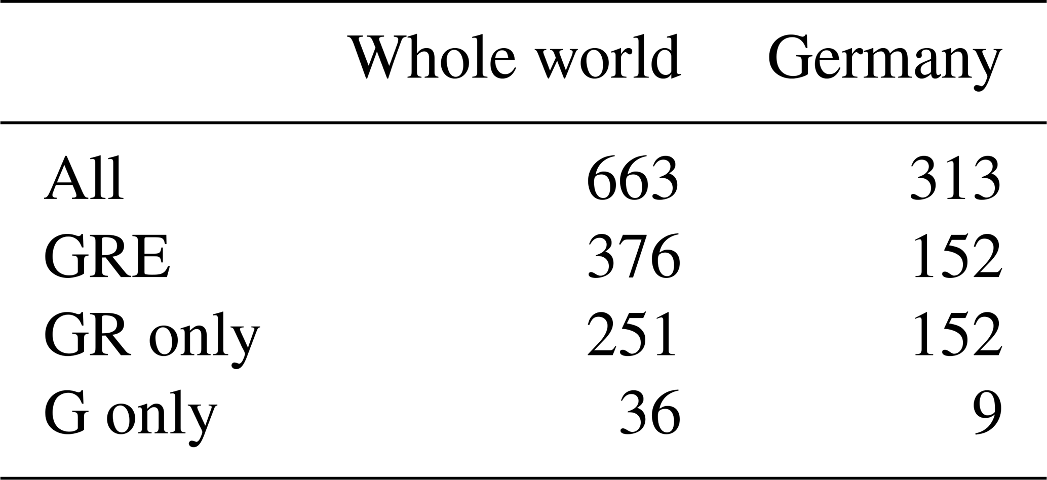
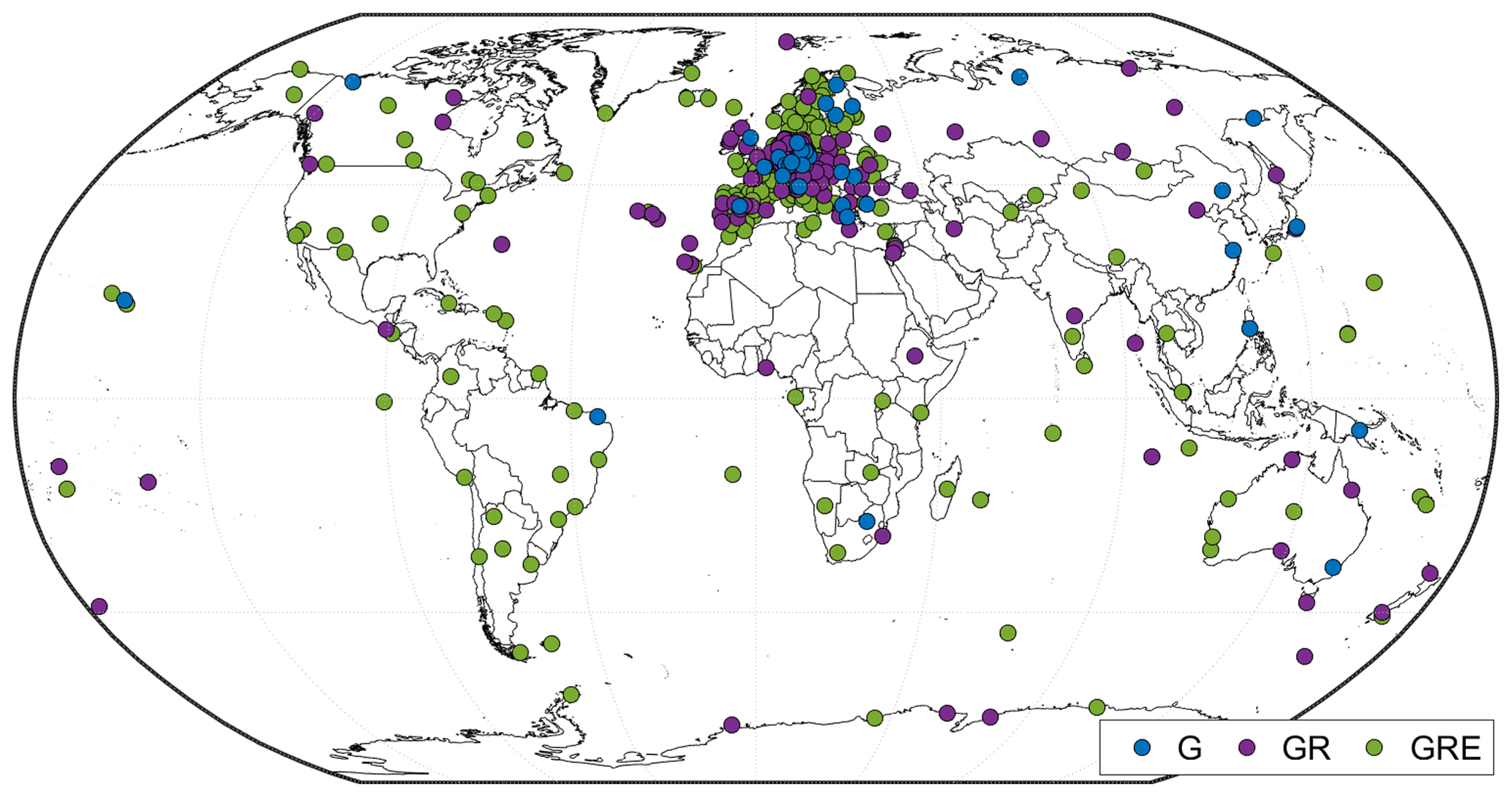
Figure 1Global map showing all stations used in this study. The colors indicate the capability to receive signals from the particular GNSS.
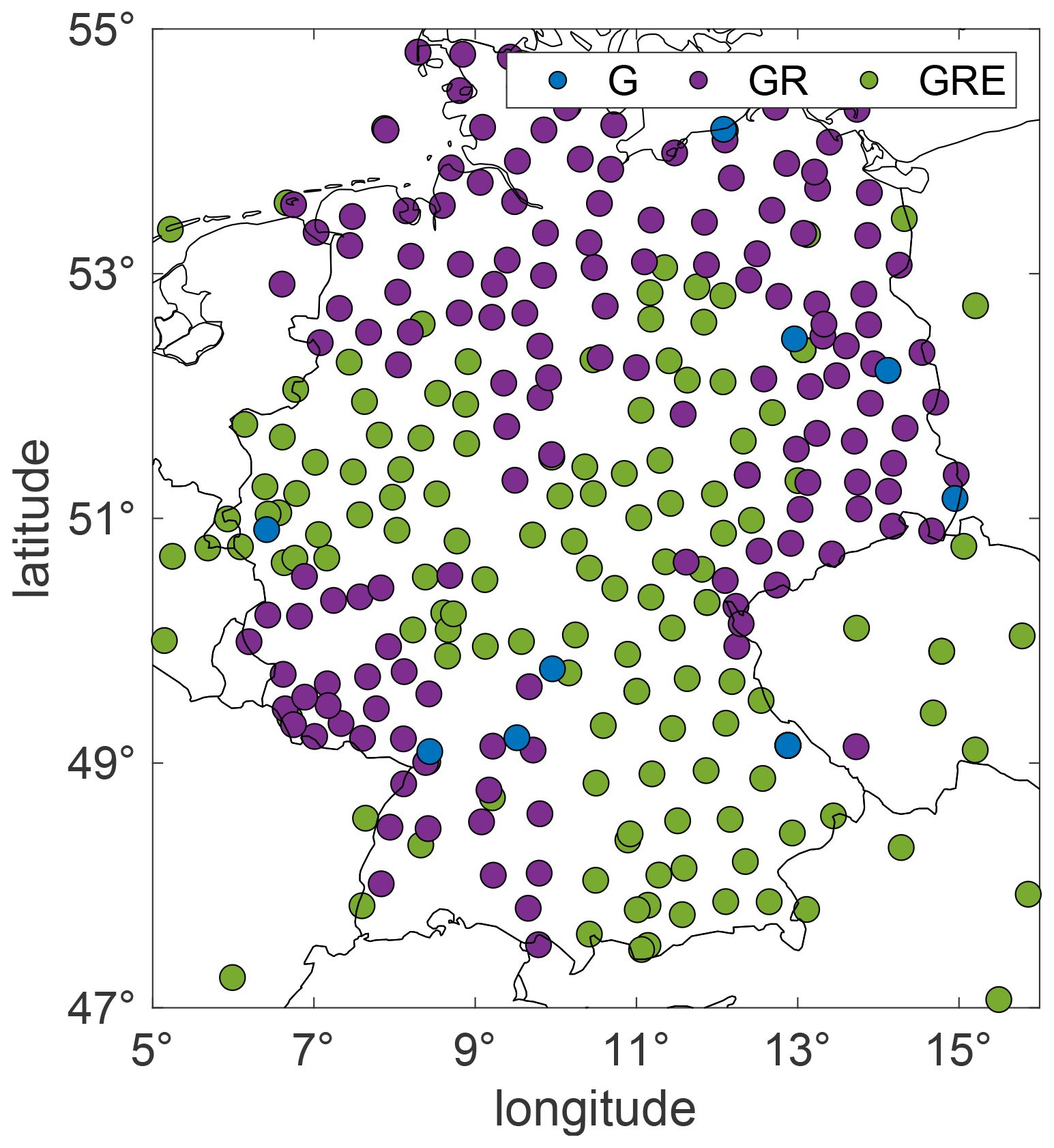
Figure 2Map of the stations used for Germany. The colors indicate the capability to receive signals from the particular GNSS.
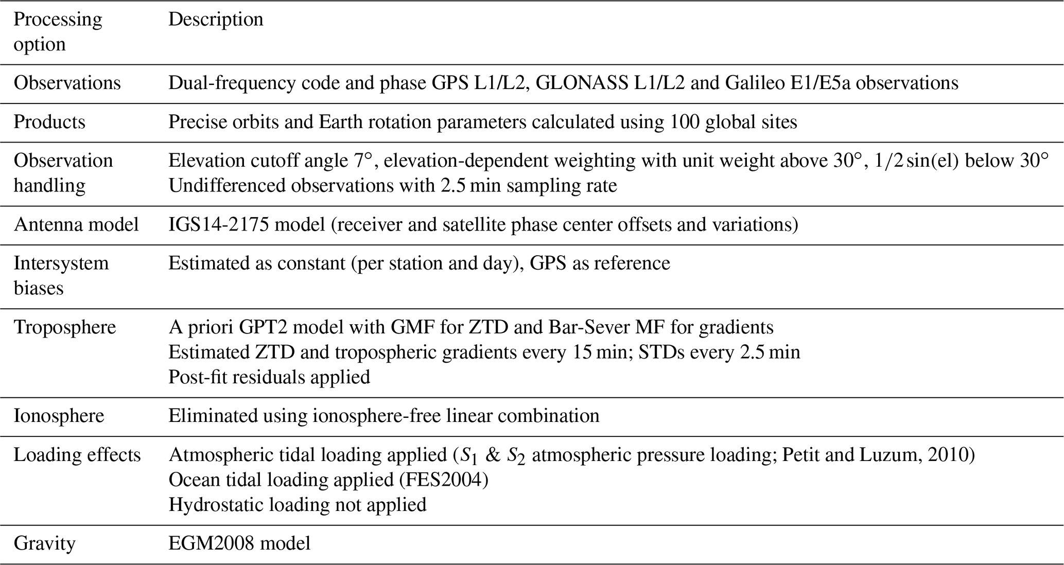
The data are processed with the EPOS.P8 software developed at GFZ (Dick et al., 2001; Gendt et al., 2004; Wickert et al., 2020) in the post-processing mode using the precise point positioning (PPP) technique. The tropospheric parameters are adjusted using the 24 h data intervals with the sampling rate of 15 min for ZTD and tropospheric gradients. The post-fit residuals are used for the calculation of STDs with a 2.5 min sampling rate. In the preprocessing step, the GFZ high-quality orbits and clocks are estimated using a base of approx. 100 stations located uniformly around the world. The a priori ZHDs are taken from the Global Pressure Temperature 2 (GPT2) model (Böhm et al., 2007; Lagler et al., 2013), and the mapping function for the ZTD is the Global Mapping Function (GMF) (Böhm et al., 2006). The mapping function for tropospheric gradients is calculated according to Bar-Sever et al. (1998); i.e., the wet mapping function is multiplied by the cotangent of the respective elevation angle. More processing information can be found in Table 2.
Petit and Luzum, 2010Table 2Characteristics of the multi-GNSS processing at GFZ for this study.
3.2 NWM data
The GNSS estimates are compared with the data from the fifth-generation ECMWF reanalysis (ERA5; http://www.ecmwf.int/en/forecasts/datasets/reanalysis-datasets/era5, last access: 17 December 2021). The ERA5 data are provided with a horizontal resolution of 0.25∘ × 0.25∘ on 31 pressure levels. The data are provided with a 3-month delay; however the preliminary data sets are published with a delay of 5 d. The temporal resolution used in this study is 1 h for ZTDs and tropospheric gradients and 6 h for STDs (to reduce the computational cost and the data volume). There is no ground-based GNSS data assimilation in the model, but the GNSS radio occultation (RO) data are assimilated (Healy et al., 2005).
The ERA5 provides gridded pressure, temperature and humidity fields. Hence, in the first step, the gridded refractivity field is computed using Eq. (2). Then, the refractivity at any arbitrary point is obtained by interpolation; i.e., for some arbitrary point, the four surrounding refractivity profiles are identified, and for each refractivity profile, a logarithmic interpolation adjusts the refractivity vertically, and then a bilinear interpolation including the vertically adjusted refractivity values is performed (Zus et al., 2012). This interpolation routine is the prerequisite to the computation of the tropospheric delays for arbitrary station locations (Zus et al., 2014).
The STDs for each GNSS satellite–receiver pair are calculated using the GFZ-developed ray-tracing software described in detail by Zus et al. (2014). The horizontal gradients from the ERA5 are calculated by the least-squares adjustment. The used gradient mapping function is the one proposed by Bar-Sever et al. (1998) to match the gradient mapping function that is utilized in the GNSS analysis. The exact description of the methodology of calculating gradients is presented by Zus et al. (2019).
We present the comparison of tropospheric parameters: ZTDs, tropospheric gradients and STDs obtained from three GNSS solutions with ERA5 estimates. We acknowledge that the NWMs are an imperfect reference data source; however, their global coverage makes it convenient to see how the agreement between them and the particular GNSS solutions changes. The comparisons are made for the entire year of 2020.
4.1 Comparisons of zenith total delays
At first, we show the intra-comparisons of the three GNSS solutions, and then we compare the solutions with ERA5. In the following comparisons, we take into account only the stations that are GRE compatible, i.e., 376 stations for the entire world and 152 for Germany.
4.1.1 Intra-comparisons of the GNSS solutions
We compare the GNSS estimates from the three solutions, GPS-only (G), GPS–GLONASS (GR) and GPS–GLONASS–Galileo (GRE). At first, we take a look at the formal errors of ZTDs from the three solutions. Figure 3 shows the errors averaged for each station from the entire year of 2020 as well as one value for each system, averaged from all the epochs and stations. We can see that adding GLONASS reduces the formal error from 1.22 to 0.99 mm, and adding Galileo reduces it further to 0.93 mm.
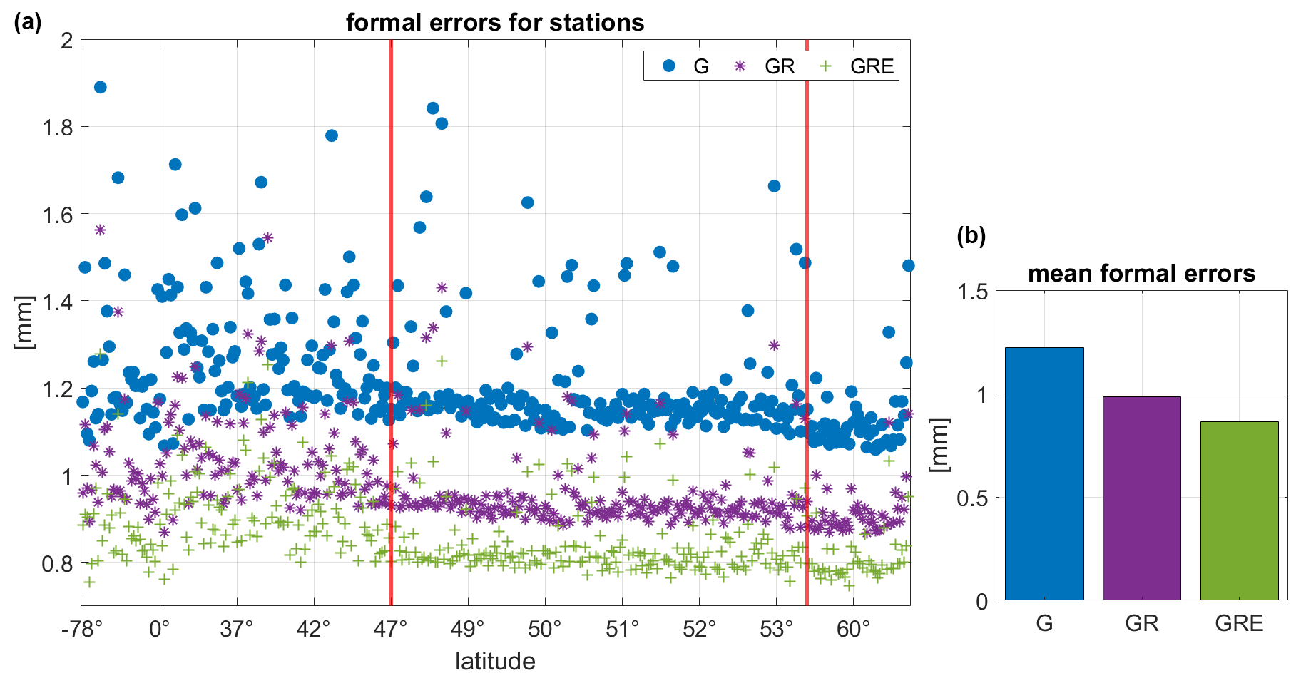
Figure 3Average formal errors of ZTD for each station in the processing (sorted by latitude, Southern Hemisphere first) (a) and the mean formal error averaged from all stations and epochs (b). The red lines indicate the latitude band that includes Germany. Please note that the labeling of the x axis is non-equidistant. The values are calculated for the year 2020.
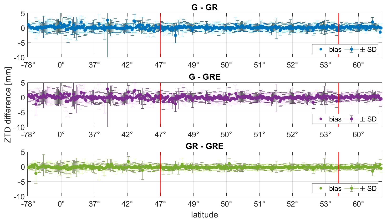
Figure 4The ZTD biases and SDs for each station (sorted by latitude, Southern Hemisphere first) between the three different GNSS solutions. The red lines indicate the latitude band that includes Germany. Please note that the labeling of the x axis is non-equidistant. The statistics are calculated for the year 2020.
Figure 4 shows the biases plus/minus their respective standard deviations (SDs) for each station (sorted by latitude, Southern Hemisphere first), and Table 3 shows the mean biases and SDs averaged from all stations.
Table 3Statistics between the particular GNSS ZTD solutions averaged from all stations for the entire year of 2020.

Figure 4 shows that the largest differences can be observed for the Southern Hemisphere and around the Equator, where the ZTD values are in general larger. The differences between particular solutions are small but existent. Table 3 shows that the biases are the largest between GR and GRE solutions for the whole world, and between GPS and GRE, as well as between GR and GRE for Germany. The SDs are the largest between GPS and GRE in both cases.
4.1.2 Comparisons with NWMs
We compare the three GNSS solutions with the ERA5 estimates. Figure 5 shows the box plots of the differences between the GNSS and ERA5. As shown in the plot, the differences between ERA5 and the GNSS for each solution exhibit similar patterns. However, the number of outliers is reduced for the GR and GRE solutions compared to the GPS-only solution. It shows that the GR and GRE solutions are less noisy. Table 4 shows the overall statistics of the differences between ERA5 and particular GNSS solutions. Figure 6 shows the biases and SDs for each station between the ERA5 model and GNSS solutions. For better visualization of the results, Fig. 7 shows the statistics for each station on a map for the entire world and Fig. 8 for Germany.
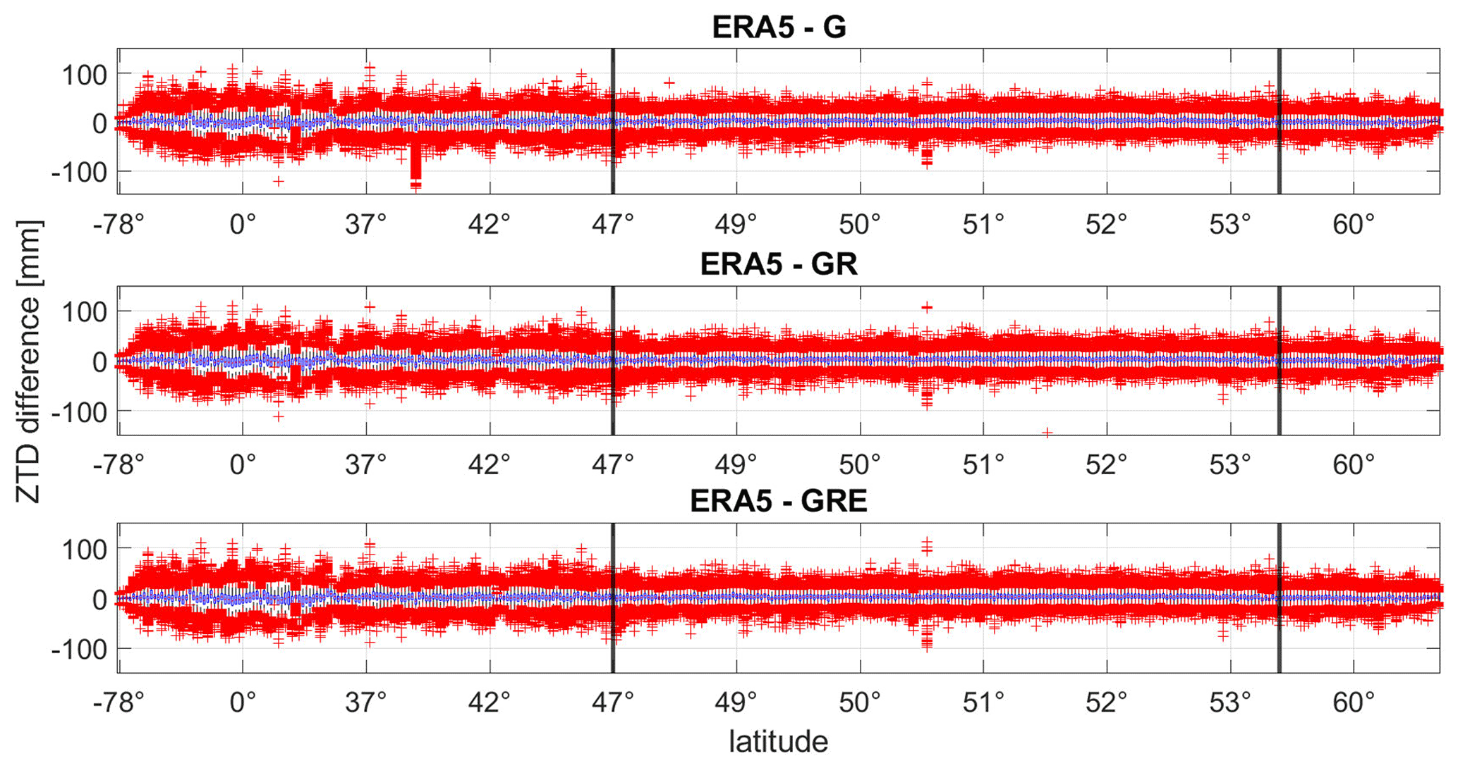
Figure 5The box plots of the ZTD differences between ERA5 and three GNSS solutions for each station. The blue boxes denote the 25th and 75th percentile. The median is marked inside the boxes. The red crosses denote outliers. The stations are sorted by latitude, and the black lines indicate the latitude band that includes Germany. Please note that the labeling of the x axis is non-equidistant. The values are calculated for the year 2020.
Table 4Statistics between the ZTD from ERA5 and GNSS solutions averaged from the year 2020 and all stations.

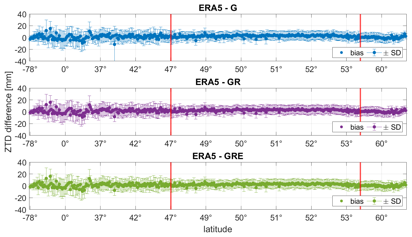
Figure 6The ZTD biases and SDs for each station (sorted by latitude, Southern Hemisphere first) between the ERA5 model and three different GNSS solutions. The red lines indicate the latitude band that includes Germany. Please note that the labeling of the x axis is non-equidistant. The statistics are calculated for the year 2020.

Figure 7The map of ZTD biases and SDs for each station between the ERA5 model and three different GNSS solutions. The statistics are calculated for the year 2020.
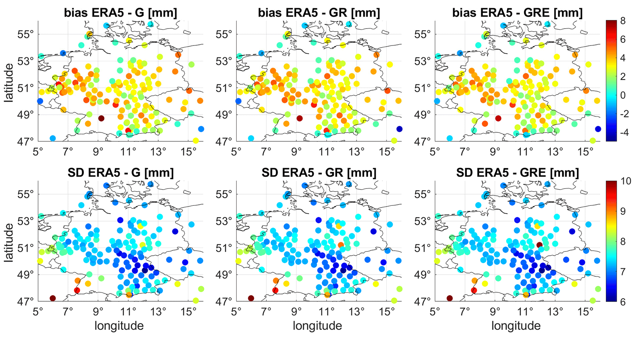
Figure 8The map of ZTD biases and standard deviations between ERA5 and the three GNSS solutions for Germany. The values are averaged from the year 2020. The map shows only the GRE capable stations; thus there are gaps for some regions.
Figure 6 shows that at the first glance, all three solutions are very similar. However, taking a closer look to the statistics in Table 4 we can see some differences. For the whole world, the biases are similar for GPS-only and GRE solutions, while for GR they are slightly larger. The SDs are slightly reduced for GR and GRE compared to the GPS-only solution. For Germany, the GRE solution has the smallest bias, but the SDs from all solutions are basically the same. Figure 7 shows the distribution of the biases and SDs on the world map. For the Northern Hemisphere, the biases are small and positive except for a few stations. The positive bias means that the ERA5 model is producing conditions that are too wet compared to the GNSS estimates. Close to the Equator, the biases are larger and negative. Here, the ERA5 model is producing conditions that are too dry with respect to the GNSS estimates. The pattern we find, i.e., the underestimation of the NWM delays around the Equator and the overestimation of the NWM delays at midlatitudes, is in good agreement with the results reported by Bock and Parracho (2019). The SDs are also larger close to the Equator, where the values of the ZTDs are in general larger due to higher humidity, which makes it more difficult to predict the values from NWMs as well as estimate them with GNSS data.

Figure 9The ZTD difference values for station POTS (Potsdam, Germany) between the three GNSS solutions: GPS-only, GR and GRE and ERA5 model (top) and histograms of the differences between the particular solutions and models (bottom). The plots are shown for the year 2020.
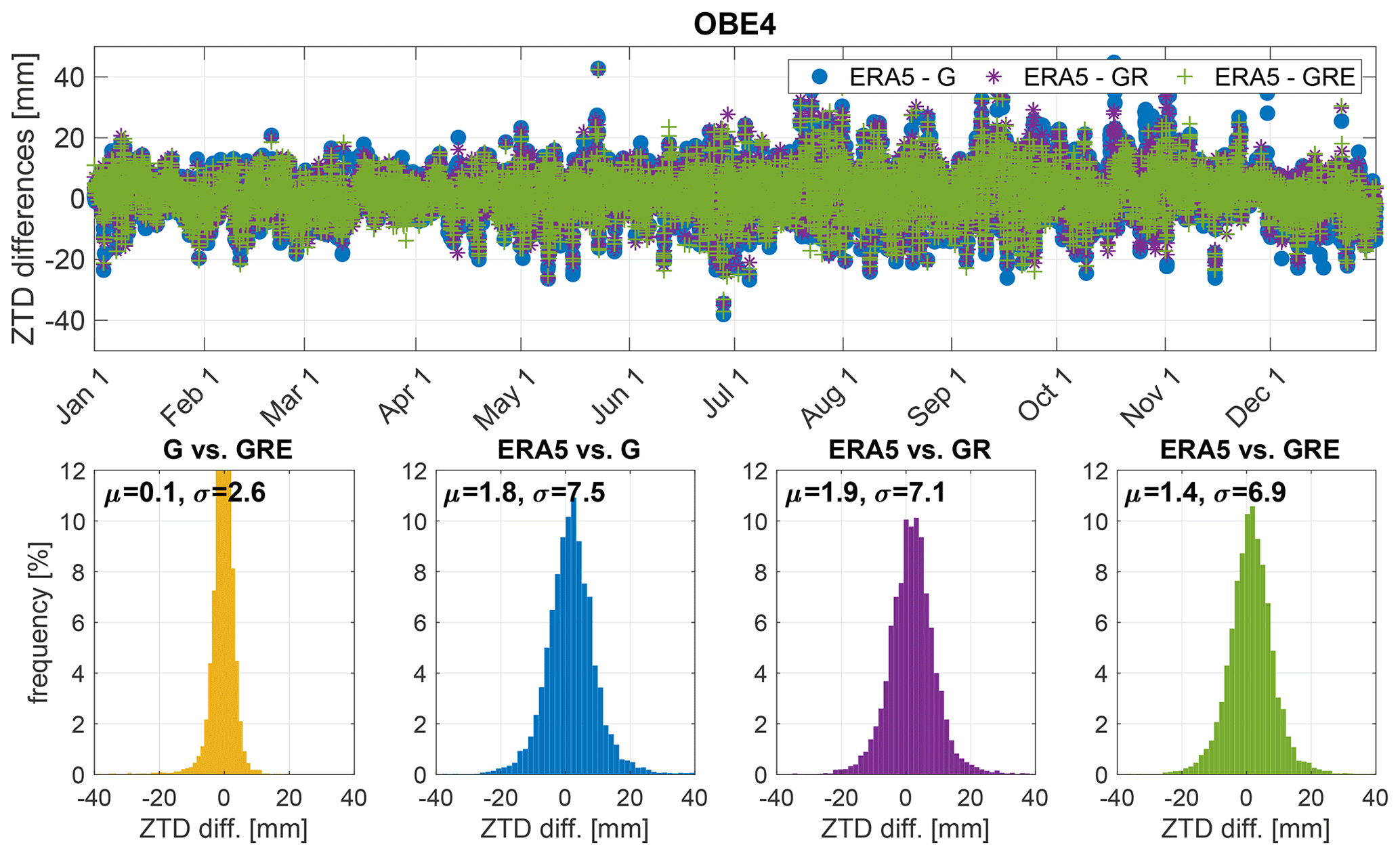
Figure 10The ZTD difference values for station OBE4 (Oberpfaffenhofen, Germany) between the three GNSS solutions: GPS-only, GR and GRE and ERA5 model (top) and histograms of the differences between the particular solutions and models (bottom). The plots are shown for the year 2020.
Figure 8 shows larger, positive biases for the western part of Germany, while in the eastern part they are smaller. Only for a few stations are the biases negative. The SDs are almost identical for most of Germany (about 6–8 mm). The differences between particular solutions are not large, but for some stations, especially in the south and west of Germany, both biases and SDs are slightly reduced for the GRE solution. Figures 9 and 10 show the ZTD differences between the three GNSS solutions and ERA5, as well as the histograms of the residuals for two sample stations: POTS (Potsdam, Germany) and OBE4 (Oberpfaffenhofen, Germany), respectively.
Both POTS and OBE4 have large, positive biases and SDs with respect to the ERA5. For the station POTS (Fig. 9), we can observe a reduction of bias of around 1.5 mm for GRE compared to the GPS-only solution, while the SDs remain at the same level. For the station OBE4 (Fig.10) there is a small reduction of both the biases and SDs.
4.2 Comparisons of tropospheric gradients
The tropospheric gradients are a measure of anisotropy in the north–south (GN) and east–west (GE) directions. The gradients are of small magnitude, typically below 3 mm. Table 5 shows the biases, SDs and Pearson's correlation coefficients (R) between the three GNSS solutions averaged from all the stations and epochs, and Table 6 shows the same statistics but between ERA5 and the three GNSS solutions.
Table 5Biases, SDs and Pearson's correlations between the three GNSS solutions for tropospheric gradients averaged from the year 2020 and all stations.

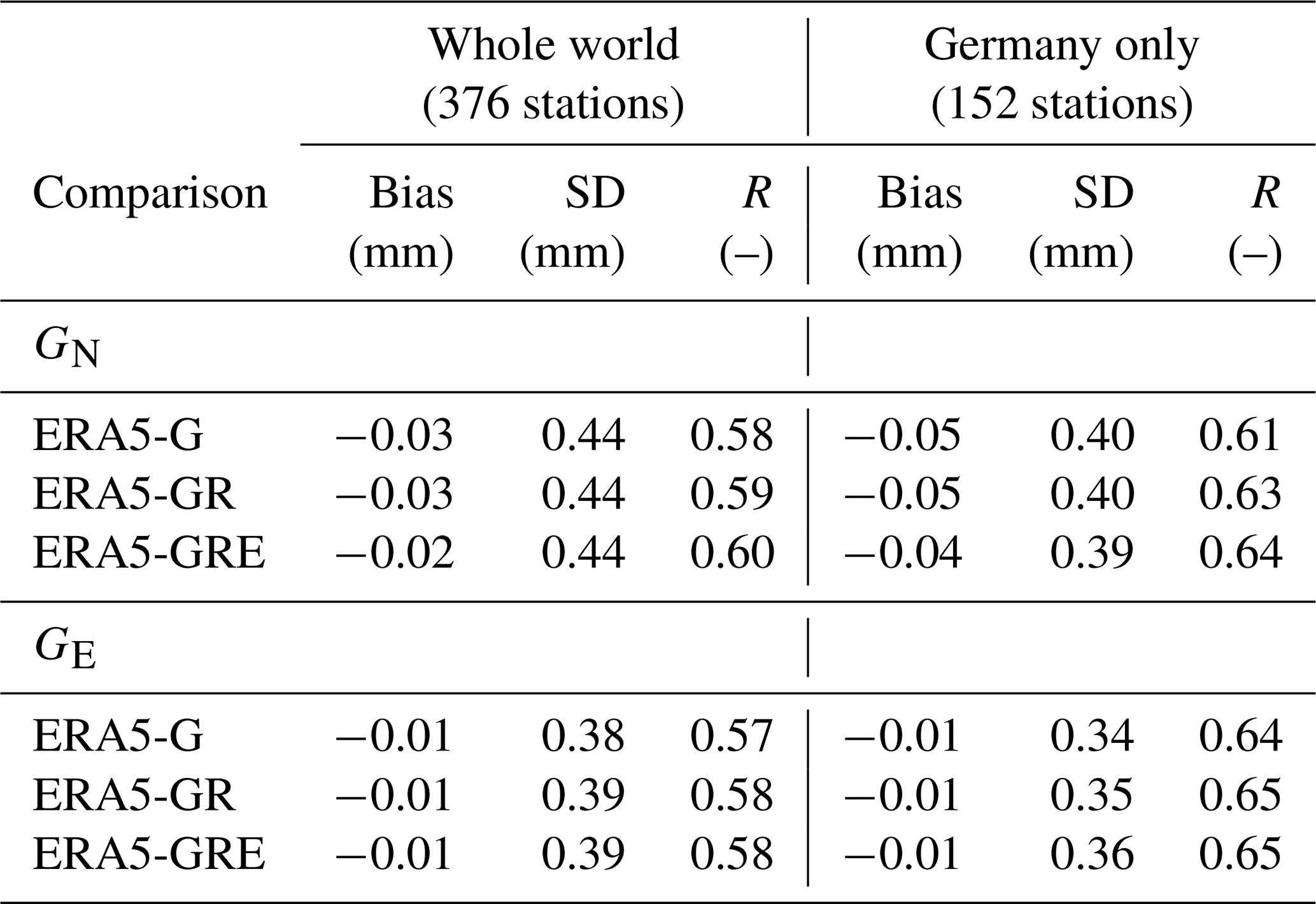
Table 6Biases, SDs and Pearson's correlations between the ERA5 and GNSS solutions for tropospheric gradients averaged from the year 2020.
As shown in Table 5, the biases between the particular solutions are very close to zero, and SDs are of 0.1–0.2 mm. The largest SDs are between GRE and GPS-only solutions, which was expected. For Germany, the SDs are slightly smaller than for the whole world. The correlations between the solutions are high, around 0.9–1.0, and are the highest between GR and GRE solutions and the lowest between GPS-only and GRE.
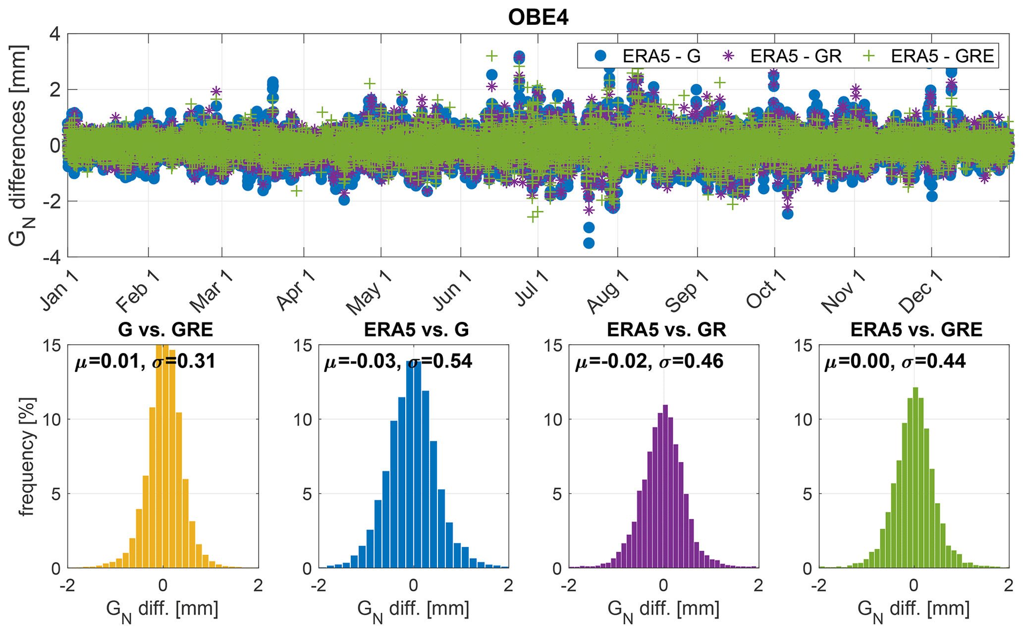
Figure 11The GN differences between the three GNSS solutions: GPS-only, GR and GRE and ERA5 for station OBE4 (Oberpfaffenhofen, Germany) (top) and the histograms of the differences (bottom). The statistics were calculated from the year 2020.

Figure 12The GE differences between the three GNSS solutions: GPS-only, GR and GRE and ERA5 for station OBE4 (Oberpfaffenhofen, Germany) (top) and the histograms of the differences (bottom). The statistics were calculated from the year 2020.
The values in Table 6 are a few times larger than in Table 5. They may still seem small, but please note that, with the exception of severe weather conditions, the values of gradients are usually below 1 mm. The SD of around 0.4 mm can actually constitute 40 % or more of the entire gradient value. Thus, the differences between ERA5 and GNSS gradients are considered significant. The biases are however still rather small. Moreover, the differences between the particular GNSS solutions are not pronounced. The correlation coefficients are slightly higher for the GRE solution. For Germany, the biases are larger than for the entire world, but the SDs are smaller. The correlation coefficients are also a bit larger for Germany, where the gradients are more consistent. We do not show the plots analogical to Figs. 4 and 6 but would like to mention that the statistics (mostly SDs) are also larger for the Southern Hemisphere and close to the Equator, but the magnitude is smaller than for ZTDs. To give an example of the gradients' behavior, we plot them for a sample station OBE4. Figure 11 shows the differences between ERA5 and GNSS for the north–south gradient and Fig. 12 for the east–west gradient.
Figures 11 and 12 do not show a visible offset between the ERA5 and GNSS values like in the case of ZTD. The tropospheric gradients, especially from the GNSS, are much more varying and harder to predict than ZTDs. For this particular station (OBE4), there is a slight reduction of bias and a larger reduction of SD for the both GR and GRE solution compared to the GPS-only solution for GN, as well as a reduction of bias and SDs for the GE. This shows that for some particular stations, using more systems is more beneficial than just using GPS also for tropospheric gradients.
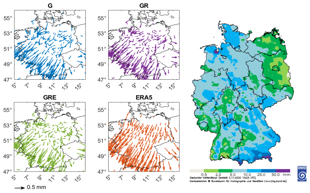
Figure 13The tropospheric gradients from the three GNSS solutions and ERA5 for Germany for a chosen date: 29 October 2020, 12:00 UTC (left panel). The right panel shows a map of precipitation for Germany on that day (source: DWD).
Both gradient components form a vector which points to the local maxima of tropospheric correction, and this usually corresponds to the increasing water vapor content (Douša et al., 2016). To visualize that, Fig. 13 shows gradients for one chosen date, 29 October 2020, 12:00 UTC. On that day, a considerable amount of rain, especially in the southwest of Germany, was observed (up to 50 mm d−1 in southern Bavaria). The figure also contains a map of the precipitation for Germany on that day.
The tropospheric gradients from ERA5, as shown in Fig. 13, exhibit a clear pattern, pointing to the southeast direction for almost the entire country. The GNSS gradients appear more noisy, especially in northeastern Germany. However, all the GNSS solutions are very similar. In general, they also point in the same direction as the ERA5 gradients, especially in southeastern Germany, where the gradient magnitudes are much larger. For this part of the country, all the ERA5 gradients clearly changed direction, but the GNSS gradients do not reconstruct this behavior so clearly.
4.3 Comparisons of slant total delays
From the information in the zenith direction, the tropospheric gradients and the post-fit residuals, the GNSS STDs are derived (Eq. 4). We compare the STDs from the three GNSS solutions with the ray-traced STDs from ERA5 model. Please note that due to the coarse temporal resolution of ERA5 and computational costs, the ray-traced STDs are calculated only four times per day. Moreover, we take the information from all the stations depicted in Figs. 1 and 2 (i.e., 663 stations for the entire world and 313 stations for Germany) because for STDs we have a separate solution for each satellite–station pair; thus there is no need to exclude any specific stations. Figure 14 shows the differences between the three solutions and the ERA5 estimates for each elevation angle and the statistics derived from the comparison.
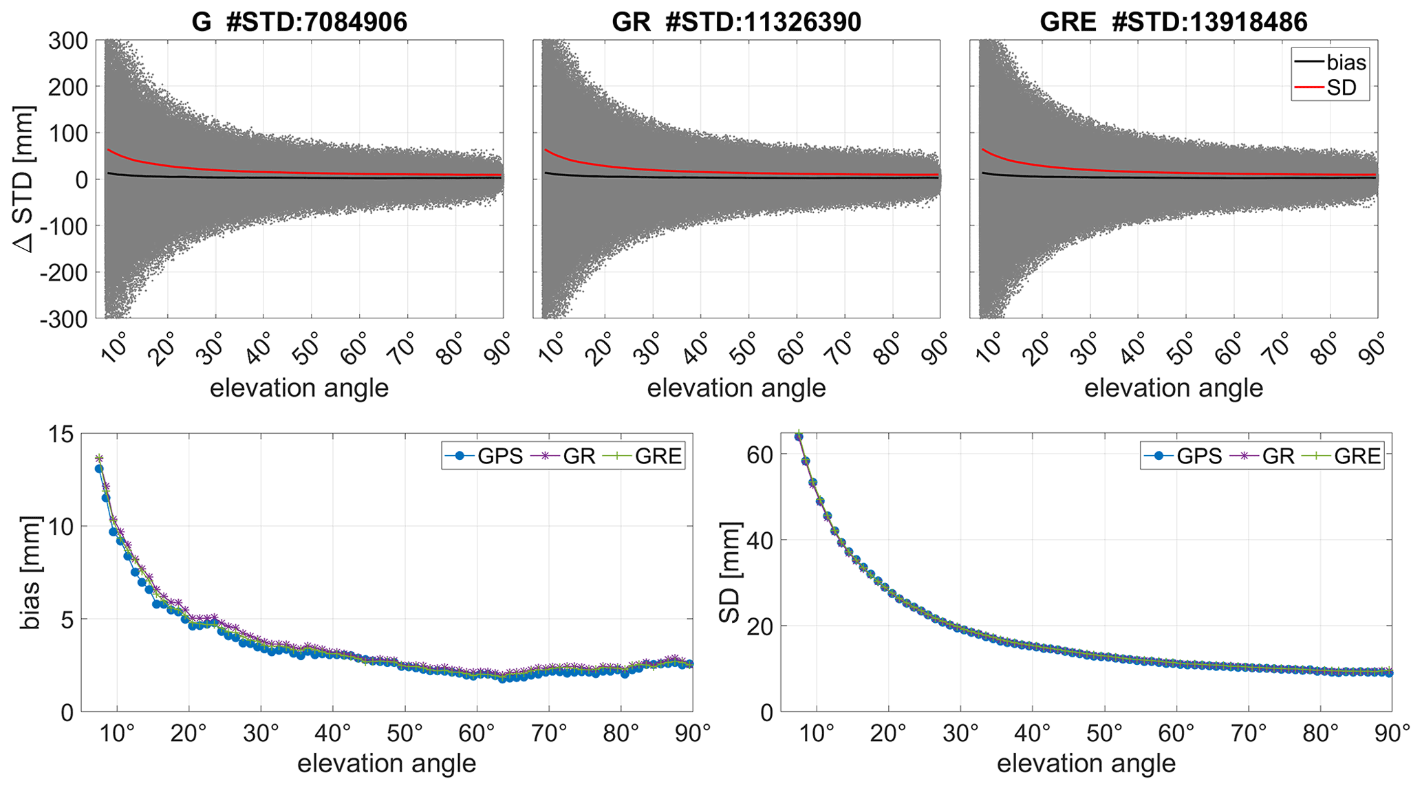
Figure 14The STD differences between ERA5 and three GNSS solutions for the year 2020 for all 663 stations with marked average biases and SDs (top) and the averaged biases and SDs from all solutions altogether (bottom).
Figure 14 shows larger differences for low elevation angles than close to the zenith. This is due to the fact that the STDs for low elevation angles (here the cutoff angle is 7∘) are around 10 times larger than at zenith. Thus, also the residuals for the low elevation angles are much larger. We can also see that the number of observations is higher for GRE or GR than for GPS-only, but the shape of the curves is very similar for all three solutions. The average SDs are also almost identical for all solutions; however, the biases differ slightly, with the smallest biases obtained from the GPS-only and GRE solutions and the largest from GR.
Table 7The STD biases and standard deviations between ERA5 and three GNSS solutions (whole world: 663 stations). The statistics are calculated four times per day (at 00:00, 06:00, 12:00, and 18:00 UTC) and averaged over the year 2020.
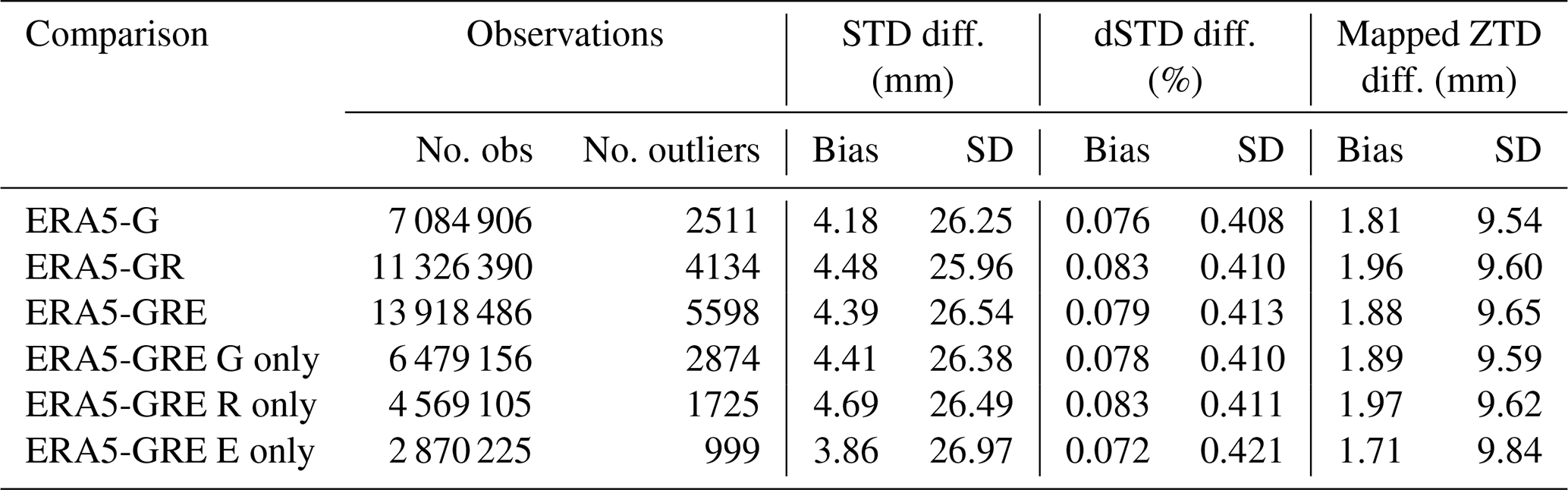
Table 7 shows the statistics for the entire world for the differences between the GNSS solutions and ERA5 model. Due to the fact that the STD values are much larger for low elevation angles, we also show the statistics for the relative differences (dSTDs), which are obtained by dividing the differences by the GNSS STD value as well as for the mapped ZTDs. These ZTDs are calculated using a simple mapping function; i.e., . The simple MF is used here just to project the results to the zenith direction to make them more comparable. To calculate the STDs, the GMF is used as described in Sect. 3.1. Table 7 also consists of the statistics for the GPS-, GLONASS- and Galileo-only products that are extracted from the GRE solution. Table 9 shows the analogous parameters but averaged from the German stations.
Table 8The STD biases and standard deviations between ERA5 and the GRE solution with and without post-fit residuals. The statistics are calculated four times per day (at 00:00, 06:00, 12:00, and 18:00 UTC) and averaged over October 2020.
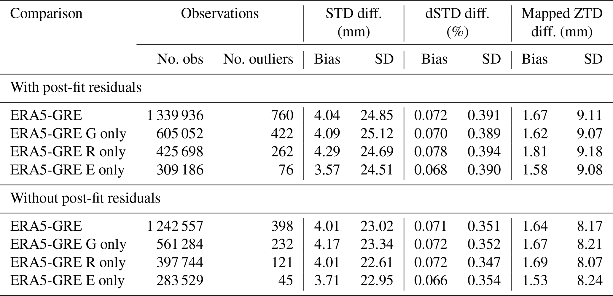
Table 9The STD biases and standard deviations between ERA5 and different GNSS solutions (for Germany: 313 stations). The statistics are calculated four times per day (at 00:00, 06:00, 12:00, and 18:00 UTC) and averaged over the year 2020.

As shown in Table 7, the agreement is at a similar level for all solutions. However, it is slightly worse for the GR and GRE solutions, compared to GPS-only solution. If we consider each system separately (from the GRE solution), we can see that actually the Galileo-only solution has the smallest biases. The biases and SDs in Table 7 may appear quite large, but when we calculate the average relative statistics, the biases from different solutions are around 0.07 % and SDs around 0.4 %. They are following the same patterns as the absolute statistics; i.e., the GPS-only solution has the best agreement, but the bias is the smallest from the Galileo-only solution. The biases for the mapped ZTDs are very similar to the ones presented in Sect. 4.1, but the SDs are a bit larger. One reason is the usage of the simple mapping function, which may deteriorate the results (Shehaj et al., 2020). The other possible reason may be adding the phase post-fit residuals, which may introduce more noise to the solution. The usage of the post-fit residuals may also be the reason why the biases from Galileo-only solution are the smallest. The Galileo clocks are more stable than GPS and GLONASS, which is beneficial for the PPP approach, and consequently the Galileo residuals are smaller and contain less noise. However, not all studies consistently conclude that post-fit residuals should be added when reconstructing the STDs (e.g., Zus et al., 2012; Kačmařík et al., 2017). The post-fit residuals contain some tropospheric information, but the residuals can also be noisy, hence deteriorating the reconstruction of STDs. To show the impact of the post-fit residuals, we calculate the STDs with and without the residuals for the month of October 2020 for the GRE solution. Table 8 shows the statistics for the two solutions.
Table 8 shows that the differences between ERA5 and GNSS solutions are in general smaller without the post-fit residuals. This is due to two facts: (1) ERA5 has a sparse horizontal resolution, so it does not resolve small-scale water vapor well; and (2) residuals contain mostly noise, especially for high elevation angles. However, in cases of severe weather events, there may be more tropospheric information in the residuals, which can have more positive influence on the NWM assimilation. Thus, we keep the post-fit residuals in our operational computations. Moreover, the usage of post-fit residuals has the largest impact on the Galileo solutions. We can see that when using the post-fit residuals, the bias for the Galileo-only solution is more significantly reduced compared to the solutions from other systems. For the solution without residuals, the biases for Galileo-only are also reduced but less significantly. Thus, the post-fit residuals from the Galileo system contain less noise and more information than from the other systems.
Table 7 also shows the total number of observations and detected outliers calculated using Chauvenet's criterion. Most of the outliers are found in the GRE solution for GPS observations, even though for the GPS-only processing there were not that many of them, which shows that processing GPS-only data and extracting the GPS-only data from the GRE solution results in different estimates.
For Germany only, as shown in Table 9, we have slightly worse biases than for the whole world (because here the residuals mostly have the same sign, so the biases do not cancel out), but the SDs are somewhat smaller. The statistics are following a similar pattern as for the entire world: the best agreement is still for the GPS-only solution. However, for the separate systems in the GRE solution, the GPS has the best agreement and not Galileo as in the case of the entire world. The statistics for the relative STDs and mapped ZTDs do not show the same agreement as for the absolute STDs. Here, the biases for GPS-only and GRE solutions are more similar, and only for GR are they higher, while the SDs are similar for GR and GRE. The reason may be that for GR we have more observations for low elevation angles, which being mapped with the simple MF can give larger discrepancies.
Figure 14 shows that the differences between the ERA5 and GNSS estimates depend strongly on the elevation angle. To remove this dependence, we plot in Fig. 15 the relative differences between the model and the GNSS solutions, as well as the number of observations for each elevation angle batch.

Figure 15The STD relative differences between ERA5 and the three different GNSS solutions: GPS-only, GR and GRE (top panels) and the number of observations with respect to the elevation angle for each solution (bottom). The differences are calculated for the entire year of 2020.
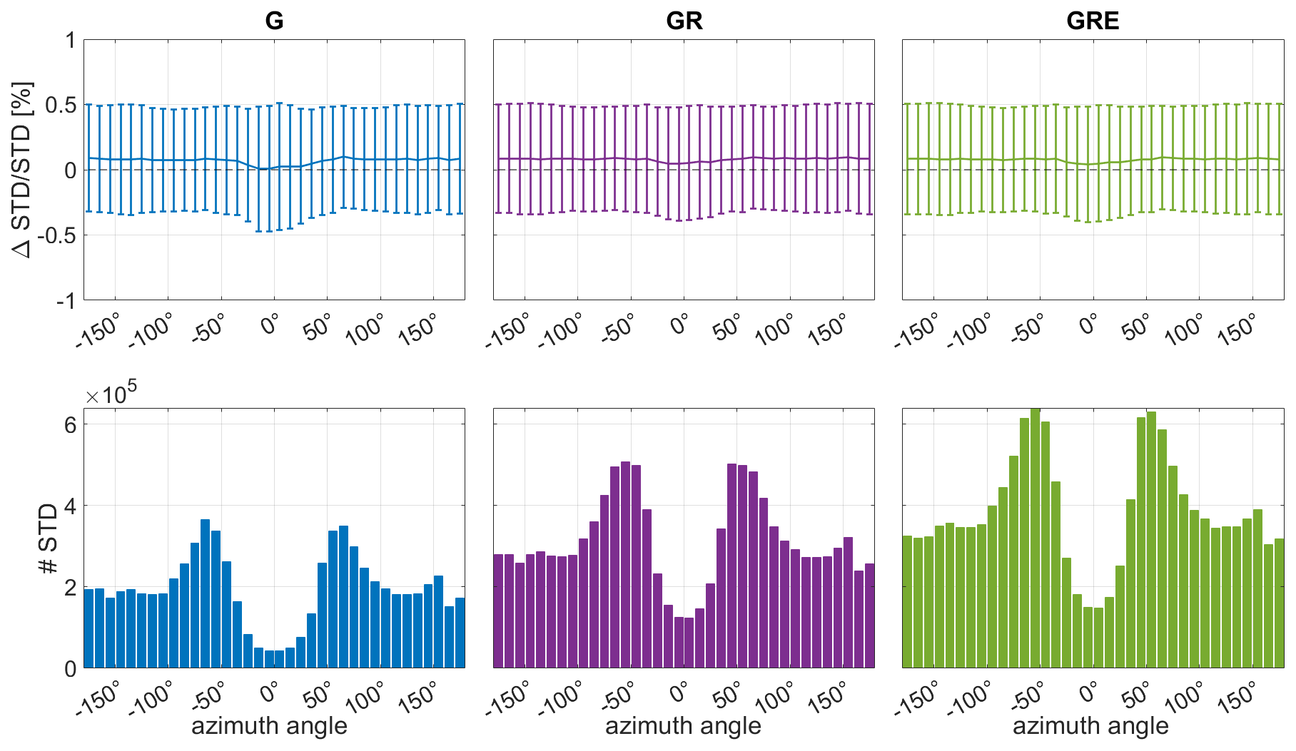
Figure 16The STD relative differences between ERA5 and the three different GNSS solutions: GPS-only, GR and GRE (top panels) and the number of observations with respect to the azimuth angle for each solution (bottom). The differences are calculated for the entire year of 2020.
Figure 15 shows that the relative differences are almost independent from the elevation angle, which means that the solutions are of equal quality for all angles. Only close to zenith do the solutions tend to deteriorate due to the limited number of observations for such angles. The differences between the solutions are rather small as shown in Table 7. Furthermore, one of the advantages of combining the solutions is the increase of the number of observations. Figure 15 shows that adding particular systems increases the number of observations significantly. For this yearly comparison with 6 h resolution, we use over 7 million GPS, 4 million GLONASS and 3 million Galileo observations. Thus, the total number of GRE observations has doubled compared to the GPS-only observations. It is especially important that the number of observations for lower elevation angles is increased. For the lowest bin in Fig. 15, there are around 110 000 observations for GPS, 170 000 for GR and 230 000 observations for GRE. But also the middle bins are significantly improved, from around 100 000 observations for GPS-only to around 250 000 for GRE. The STDs depend not only on the elevation angle, but also on the azimuth angle of the satellite (see Eq. 4). Figure 16 shows the relative differences with respect to the azimuth angle and the number of observations for each angle bin.
Figure 16 shows that the relative differences depend on the azimuth angle, especially for the GPS-only solution and low azimuth angles. The reason is, as shown in the bottom panel, that there are only very few observations for azimuth angles close to 0. Adding GLONASS and Galileo observations fills this gap a little and makes the differences less dependent on the azimuth angle. Thus, adding more systems to the solution increases not only the number of low elevation angle observations but also low azimuth angle, making the observations more uniformly distributed. To sum up, we can conclude that even though adding more systems does not significantly improve the agreement between the GNSS and ERA5 solutions, it increases the number of observations, especially for low elevation and azimuth angles. This addition may lead to more precise information about the tropospheric state obtained via, e.g., water vapor tomography.
Comparisons of the GNSS and NWM estimates have already been vastly described in the literature. The majority of the studies focus on the parameters in the zenith direction, either ZTDs or IWV. Examples have been given in the Introduction of this article. Some of these studies have been conducted at GFZ or use the GFZ products. In this section, we would like to summarize a few selected studies and compare our outcomes with theirs.
Douša et al. (2017) compared the tropospheric GPS-only products calculated at 172 stations from almost 20 years of data (1996–2014) of the second EUREF reprocessing (Repro2). The ZTD comparisons with ERA-Interim reanalysis for almost all variants showed biases of 2 mm and SDs of 8 mm, which exactly corresponds with the findings of this study for the whole world. For Germany only, the biases are 3 mm with 7 mm SDs. For the GN gradient, the bias was very close to 0, with a SD of 0.4 mm, and for the GE gradient, it was −0.05 mm, with a SD of 0.4 mm. The SDs in this study correspond with the Repro2 study by Douša et al. (2017); however, our GN absolute biases are slightly larger (−0.03 mm), and the GE biases are smaller (−0.01 mm).
Kačmařík et al. (2019) studied different settings of tropospheric gradients for a COST Action ES1206 benchmark period (May–June 2013) for 430 stations in central Europe. The settings included eight different variants of processing gradients with different mapping functions, elevation cutoff angle, GNSS constellation, observations' elevation-dependent weighting and the processing mode. One of the variants concerned the GPS-only vs. the GPS–GLONASS solutions. The comparison with the NWM showed that a small decrease in the SD of the estimated gradients (2 %) was observed when using GPS–GLONASS instead of GPS-only. In our study, there is no general improvement while taking the GR or GRE solutions with respect to the GPS-only solutions. However, some selected stations, e.g., OBE4, showed a decrease of the SDs. Lu et al. (2016) compared gradients from multi-GNSS solution validated with the ECMWF NWM from 120 stations for 3 months in 2014. At that time, only eight Galileo satellites were in use. The results demonstrated that GLONASS gradients achieved comparable accuracy to the GPS gradients but had slightly more noise and outliers. Compared to the GPS- and GLONASS-only estimates, the correlation for the multi-GNSS processing was improved by about 21.1 % and 26.0 %, respectively. These results do not correspond fully with the findings of our study, where the gradients from all three solutions exhibit a similar level of agreement with the NWM. The correlation between GNSS and NWM data is improved by only 3 % for GRE compared to GPS-only solution. The reason for higher reduction in these studies and smaller reduction in our study is most probably the usage of different ways of constraining the parameters. Kačmařík et al. (2019) and Lu et al. (2016) used loose constraining, while in our study the gradients are more tightly constrained between epochs but more loose in the general magnitude.
Kačmařík et al. (2017) showed the comparisons of STDs from seven different institutions. The authors validated 11 solutions obtained using five different GNSS processing software packages. They checked different processing strategies, elevation cutoff angle, mapping functions, products used, intervals of calculating the parameters or the usage of post-fit residuals. The tests were performed for 10 reference stations of the COST Action ES1206 benchmark in 2013. This study was restricted to GPS-only and GPS–GLONASS solutions. Amongst the comparisons of many different aspects, it also showed that changing the setting from GPS-only to GPS–GLONASS resulted in the mapped ZTD bias of 0.18 mm and SD of 1.95 mm between the solutions, which is very similar to the current study. GFZ also provided their contribution to the study of Kačmařík et al. (2017), although at that time with a GPS-only solution. This was compared to the NWMs (the GFS and ERA-Interim models). The biases for the mapped ZTDs varied for different stations between 4–12 mm with SDs of 7–12 mm for GFS and 0–6 mm with 10–17 mm SDs for ERA5. The agreement is worse than in the current study (for Germany, the mapped ZTDs biases are 3 mm with SDs of 7.5 mm), probably due to the usage of the data in the warm season (and not the entire year like in this study) and possibly also due to the different way of calculating the STDs from NWMs (the assembled and not the ray-traced tropospheric delays were utilized). The study of Kačmařík et al. (2017) also showed the impact of using the post-fit residuals. The SDs between the solution with and without residuals were at a level of 4 mm with almost zero bias. In our study, we calculate the statistics between the ERA5 and the two solutions. They show that the impact of the post-fit residuals is somehow smaller and that the biases differ only by less than 0.5 mm and the SDs by about 2 mm.
Li et al. (2015a) described real-time comparisons of ZTDs, gradients, STDs and IWVs from 100 globally distributed stations and a 180 d period in 2014 and compared them to the ECMWF operational analysis. In this study, the data from four systems were considered: GPS, GLONASS, Galileo and Beidou (GREC). However, the Galileo data were very limited; there were only four satellites in the constellation. Our study is an extension of this previous study with a fully developed Galileo constellation. Moreover, Li et al. (2015a) used real-time PANDA software, while we use the operational EPOS.P8 software. The ECMWF vs. GREC ZTD comparisons resulted in a fractional bias of 0.1 % and SD of 0.5 % (corresponding to around 2 and 12 mm), which is a bit worse than in the current study (with the biases of also 2 mm and SDs of 8.5 mm). For gradients (although calculated every 12 h, not every 15 min like in this study), the authors calculated the root-mean-square error (RMSE), which equaled 0.34 mm for GREC and 0.38 mm for GPS-only, which was an 11.8 % improvement. We do not see such a behavior for our gradients; they are at a similar level for all solutions. The reason may again be that the gradients from Li et al. (2015a) are very loosely constrained, like in Kačmařík et al. (2019) and Lu et al. (2016), and this is not the case for our analysis. For the STDs, the authors do not give specific numbers, but visually the GPS-only and GREC solutions are close to each other. The SDs equaled approx. 1 cm close to the zenith and 10 cm at 7∘, which corresponds with the findings of this paper.
This study is generally in agreement with the findings of the described previous studies. The differences between NWMs and the tropospheric delays, i.e., ZTDs and STDs, are comparable. The main difference concerns the multi-GNSS gradients, which is most likely due to the different ways of constraining the gradient values. In the previous studies, mostly the estimates from GPS and GLONASS were considered, while this study additionally uses the fully operational Galileo constellation. Moreover, the software used in this study (EPOS.P8) is used to provide the tropospheric parameters to the weather services in an operational way.
This study presented a comparison of tropospheric parameters: ZTDs, tropospheric gradients and STDs from three GNSS solutions – GPS-only, GPS–GLONASS and GPS–GLONASS–Galileo with the global ERA5 reanalysis. The GNSS estimates were calculated using the GFZ-developed software EPOS.P8, providing the parameters to the weather services operationally (e.g., DWD, Met Office). The three tropospheric parameters calculated using EPOS.P8 software and the full Galileo constellation were presented in a publication for the first time. For the ZTDs, the formal error was reduced from 1.22 mm for GPS-only solution to 0.93 mm for GRE. Global comparisons with ERA5 showed biases of around 2 mm with 8.5 mm SDs. The comparisons for Germany resulted in biases of 3 mm and SDs of 7 mm, which is to be expected as for Germany the biases do not cancel out as in the case of the global network, but the estimates are more consistent. All three GNSS solutions were very similar; however, the statistics were slightly better for the GRE solution. There are some stations, e.g., POTS or OBE4, for which adding GLONASS and further Galileo reduced the biases and SDs. For the tropospheric gradients, the results from all solutions were almost identical. For GN and the global comparisons, the average bias was of around −0.03 mm with SDs of 0.4 mm and for GE the bias of −0.01 mm with 0.4 mm SDs. For Germany, the behavior was similar to the ZTDs'; i.e., the biases were slightly larger and SDs smaller. For STDs, the differences were strongly dependent on the elevation angle, with larger differences for low elevation angles and smaller values close to the zenith. The average bias was around 4 mm with 26 mm SDs, which corresponds to 0.08 % with 0.4 % SDs for the relative values. Unfortunately, for STDs, adding GLONASS and Galileo did not improve the agreement but even slightly worsened it. However, if we consider only the Galileo observations in the GRE solution, the bias was slightly reduced. For Germany, the statistics were again worse for biases and better for SDs. We also analyzed the relative differences between GNSS and ERA5 estimates. The dependence on the elevation angle was reduced almost to zero. For the relative differences, the worst agreement was obtained for the values close to the zenith, where there are fewer observations. Moreover, the dependence on the azimuth angle was tested. For the GPS-only solution, there was a deterioration of the agreement with ERA5 for azimuth angles close to zero, where there were not so many data. Adding GLONASS and Galileo increased the number of observations for such low azimuth angles and resulted in better agreement for these angles. In conclusion, the estimates from all three solutions showed a very similar agreement with respect to the ERA5. We conclude that they are of similar quality. Nonetheless, adding more systems results in better sky coverage, especially for low elevation and azimuth angles, which leads to a better geometry for future assimilation and tomography studies.
The GNSS data are processed using the GFZ-developed software EPOS.P8. GFZ owns the intellectual property rights to the EPOS.P8 software.
The ECMWF provided the ERA5 data (https://www.ecmwf.int/en/forecasts/datasets/reanalysis-datasets/era5, Zus, 2021). The GNSS observation data are provided by the following global networks: IGS (http://www.igs.org, IGS, 2021), EPN (http://www.epncb.oma.be, EPN, 2021) and GFZ (https://doi.org/10.5880/GFZ.1.1.2020.001, Ramatschi et al., 2019). The station and satellite metadata are taken from the GFZ SEnsor Meta Information SYStem (SEMISYS, https://doi.org/10.5880/GFZ.1.1.2020.005, Bradke, 2020). The GNSS analysis results from this study can be made available upon request.
All authors contributed to the conceptualization of this study. The methodology was provided by KW, GD and FZ. KW and FZ validated the results. The investigations were performed by KW, GD and FZ. Data curation was done by GD and FZ. The original draft was written by KW and reviewed by JW, FZ and GD. The visualizations were made by KW and FZ. The project was administrated by JW, and the funding was acquired by JW and GD. All authors read and approved the final paper.
The contact author has declared that neither they nor their co-authors have any competing interests.
Publisher's note: Copernicus Publications remains neutral with regard to jurisdictional claims in published maps and institutional affiliations.
This study was performed under the framework of the Deutsche Forschungsgemeinschaft (DFG) project Advanced MUlti-GNSS Array for Monitoring Severe Weather Events (AMUSE), grant no. 418870484.
This research has been supported by the Deutsche Forschungsgemeinschaft (grant no. 418870484).
This paper was edited by Roeland Van Malderen and reviewed by three anonymous referees.
Bar-Sever, Y. E., Kroger, P. M., and Borjesson, J. A.: Estimating horizontal gradients of tropospheric path delay with a single GPS receiver, J. Geophys. Res.-Sol. Ea., 103, 5019–5035, https://doi.org/10.1029/97jb03534, 1998. a, b, c
Bender, M., Dick, G., Wickert, J., Schmidt, T., Song, S., Gendt, G., Ge, M., and Rothacher, M.: Validation of GPS slant delays using water vapour radiometers and weather models, Meteorol. Z., 17, 807–812, https://doi.org/10.1127/0941-2948/2008/0341, 2008. a
Benevides, P., Catalao, J., and Miranda, P. M. A.: On the inclusion of GPS precipitable water vapour in the nowcasting of rainfall, Nat. Hazards Earth Syst. Sci., 15, 2605–2616, https://doi.org/10.5194/nhess-15-2605-2015, 2015. a
Benjamin, S. G., Weygandt, S. S., Brown, J. M., Hu, M., Alexander, C. R., Smirnova, T. G., Olson, J. B., James, E. P., Dowell, D. C., Grell, G. A., Lin, H., Peckham, S. E., Smith, T. L., Moninger, W. R., Kenyon, J. S., and Manikin, G. S.: A North American hourly assimilation and model forecast cycle: The Rapid Refresh, Mon. Weather Rev., 144, 1669–1694, https://doi.org/10.1175/MWR-D-15-0242.1, 2016. a
Bennitt, G. V. and Jupp, A.: Operational assimilation of GPS zenith total delay observations into the Met Office numerical weather prediction models, Mon. Weather Rev., 140, 2706–2719, 2012. a, b
Bevis, M., Businger, S., Chiswell, S., Herring, T., Anthes, R., Rocken, C., and Ware, R.: GPS meteorology: Mapping zenith wet delays onto precipitable water, J. Appl. Meteorol., 33, 379–386, https://doi.org/10.1175/1520-0450(1994)033<0379:GMMZWD>2.0.CO;2, 1994. a
Bock, O. and Parracho, A. C.: Consistency and representativeness of integrated water vapour from ground-based GPS observations and ERA-Interim reanalysis, Atmos. Chem. Phys., 19, 9453–9468, https://doi.org/10.5194/acp-19-9453-2019, 2019. a
Böhm, J., Niell, A., Tregoning, P., and Schuh, H.: Global Mapping Function (GMF): A new empirical mapping function based on numerical weather model data, Geophys. Res. Lett., 33, 3–6, https://doi.org/10.1029/2005GL025546, 2006. a, b
Böhm, J., Heinkelmann, R., and Schuh, H.: Short note: A global model of pressure and temperature for geodetic applications, J. Geodesy, 81, 679–683, https://doi.org/10.1007/s00190-007-0135-3, 2007. a
Boniface, K., Ducrocq, V., Jaubert, G., Yan, X., Brousseau, P., Masson, F., Champollion, C., Chéry, J., and Doerflinger, E.: Impact of high-resolution data assimilation of GPS zenith delay on Mediterranean heavy rainfall forecasting, Ann. Geophys., 27, 2739–2753, https://doi.org/10.5194/angeo-27-2739-2009, 2009. a
Bosser, P. and Bock, O.: IWV retrieval from ground GNSS receivers during NAWDEX, Adv. Geosci., 55, 13–22, https://doi.org/10.5194/adgeo-55-13-2021, 2021. a
Bradke, M.: SEMISYS – Sensor Meta Information System, V. 4.1, GFZ Data Services [data set], https://doi.org/10.5880/GFZ.1.1.2020.005, 2020. a
Chen, G. and Herring, T. A.: Effects of atmospheric azimuthal asymmetry on the analysis of space geodetic data, J. Geophys. Res.-Sol. Ea., 102, 20489–20502, https://doi.org/10.1029/97jb01739, 1997. a
Cucurull, L., Derber, J. C., Treadon, R., and Purser, R. J.: Assimilation of Global Positioning System Radio Occultation Observations into NCEP's Global Data Assimilation System, Mon. Weather Rev., 135, 3174–3193, https://doi.org/10.1175/MWR3461.1, 2007. a
de Haan, S., van der Marel, H., and Barlag, S.: Comparison of GPS slant delay measurements to a numerical model: case study of a cold front passage, Phys. Chem. Earth Pt. A/B/C, 27, 317–322, https://doi.org/10.1016/S1474-7065(02)00006-2, 2002. a
Dick, G., Gendt, G., and Reigber, C.: First experience with near real-time water vapor estimation in a German GPS network, J. Atmos. Sol.-Terr. Phy., 63, 1295–1304, https://doi.org/10.1016/S1364-6826(00)00248-0, 2001. a
Douša, J., Dick, G., Kačmařík, M., Brožková, R., Zus, F., Brenot, H., Stoycheva, A., Möller, G., and Kaplon, J.: Benchmark campaign and case study episode in central Europe for development and assessment of advanced GNSS tropospheric models and products, Atmos. Meas. Tech., 9, 2989–3008, https://doi.org/10.5194/amt-9-2989-2016, 2016. a, b
Dousa, J., Vaclavovic, P., and Elias, M.: Tropospheric products of the second GOP European GNSS reprocessing (1996–2014), Atmos. Meas. Tech., 10, 3589–3607, https://doi.org/10.5194/amt-10-3589-2017, 2017. a, b, c
Elgered, G., Ning, T., Forkman, P., and Haas, R.: On the information content in linear horizontal delay gradients estimated from space geodesy observations, Atmos. Meas. Tech., 12, 3805–3823, https://doi.org/10.5194/amt-12-3805-2019, 2019. a
EPN: Daily GNSS data, EUREF Permanent Network, available at: http://www.epncb.oma.be, last access: 5 November 2021. a
Essen, L. and Froome, K.: The refractive indices and dielectric constants of air and its principal constituents at 24 000 Mc/s, P. Phys. Soc. Lond. B, 64, 862–875, https://doi.org/10.1038/167512a0, 1951. a
Gendt, G., Dick, G., Reigber, C., Tomassini, M., Liu, Y., and Ramatschi, M.: Near real time GPS water vapor monitoring for numerical weather prediction in Germany, J. Meteorol. Soc. Jpn., 82, 361–370, https://doi.org/10.2151/jmsj.2004.361, 2004. a
Hadaś, T., Hobiger, T., and Hordyniec, P.: Considering different recent advancements in GNSS on real-time zenith troposphere estimates, GPS Solutions, 24, 1–14, https://doi.org/10.1007/s10291-020-01014-w, 2020. a
Healy, S. B., Jupp, A. M., and Marquardt, C.: Forecast impact experiment with GPS radio occultation measurements, Geophys. Res. Lett., 32, 1–4, https://doi.org/10.1029/2004GL020806, 2005. a
IGS: Daily GNSS data, International GNSS Service, available at: http://www.igs.org, last access: 5 November 2021. a
Johnston, G., Riddell, A., and Hausler, G.: The international GNSS service, in: Springer handbook of global navigation satellite systems, Springer, Cham, Switzerland, 967–982, 2017. a
Kačmařík, M., Douša, J., Dick, G., Zus, F., Brenot, H., Möller, G., Pottiaux, E., Kapłon, J., Hordyniec, P., Václavovic, P., and Morel, L.: Inter-technique validation of tropospheric slant total delays, Atmos. Meas. Tech., 10, 2183–2208, https://doi.org/10.5194/amt-10-2183-2017, 2017. a, b, c, d, e
Kačmařík, M., Douša, J., Zus, F., Václavovic, P., Balidakis, K., Dick, G., and Wickert, J.: Sensitivity of GNSS tropospheric gradients to processing options, Ann. Geophys., 37, 429–446, https://doi.org/10.5194/angeo-37-429-2019, 2019. a, b, c, d
Kawabata, T., Shoji, Y., Seko, H., and Saito, K.: A numerical study on a mesoscale convective system over a subtropical island with 4D-var assimilation of GPS slant total delays, J. Meteorol. Soc. Jpn., 91, 705–721, https://doi.org/10.2151/jmsj.2013-510, 2013. a
Lagler, K., Schindelegger, M., Böhm, J., Krásná, H., and Nilsson, T.: GPT2: Empirical slant delay model for radio space geodetic techniques, Geophys. Res. Lett., 40, 1069–1073, https://doi.org/10.1002/grl.50288, 2013. a
Li, X., Zus, F., Lu, C., Dick, G., Ning, T., Ge, M., Wickert, J., and Schuh, H.: Retrieving of atmospheric parameters from multi-GNSS in real time: Validation with water vapor radiometer and numerical weather model, J. Geophys. Res., 120, 7189–7204, https://doi.org/10.1002/2015JD023454, 2015a. a, b, c, d
Li, X., Zus, F., Lu, C., Ning, T., Dick, G., Ge, M., Wickert, J., and Schuh, H.: Retrieving high-resolution tropospheric gradients from multiconstellation GNSS observations, Geophys. Res. Lett., 42, 4173–4181, https://doi.org/10.1002/2015GL063856, 2015b. a
Lindskog, M., Ridal, M., Thorsteinsson, S., and Ning, T.: Data assimilation of GNSS zenith total delays from a Nordic processing centre, Atmos. Chem. Phys., 17, 13983–13998, https://doi.org/10.5194/acp-17-13983-2017, 2017. a
Lu, C., Li, X., Li, Z., Heinkelmann, R., Nilsson, T., Dick, G., Ge, M., and Schuh, H.: GNSS tropospheric gradients with high temporal resolution and their effect on precise positioning, J. Geophys. Res., 121, 912–930, https://doi.org/10.1002/2015JD024255, 2016. a, b, c, d
Lu, C., Feng, G., Zheng, Y., Zhang, K., Tan, H., Dick, G., Wickert, J., and Wickert, J.: Real-time retrieval of precipitable water vapor from Galileo observations by using the MGEX network, IEEE T. Geosci. Remote, 58, 4743–4753, https://doi.org/10.1109/TGRS.2020.2966774, 2020. a
Petit, G. and Luzum, B.: IERS conventions, Tech. rep., International Earth Rotation and Reference Systems Service, Central Bureau, Frankfurt am Main, Germany, 2010. a
Poli, P., Moll, P., Rabier, F., Desroziers, G., Chapnik, B., Berre, L., Healy, S. B., Andersson, E., and Guelai, F.-Z. E.: Forecast impact studies of zenith total delay data from European near real-time GPS stations in Météo France 4DVAR, J. Geophys. Res., 112, D06114, https://doi.org/10.1029/2006JD007430, 2007. a, b
Ramatschi, M., Bradke, M., Nischan, T., and Männel, B.: GNSS data of the global GFZ tracking network, V. 1, GFZ Data Services [data set], https://doi.org/10.5880/GFZ.1.1.2020.001, 2019. a, b
Rohm, W., Guzikowski, J., Wilgan, K., and Kryza, M.: 4DVAR assimilation of GNSS zenith path delays and precipitable water into a numerical weather prediction model WRF, Atmos. Meas. Tech., 12, 345–361, https://doi.org/10.5194/amt-12-345-2019, 2019. a, b
Saito, K., Shoji, Y., Origuchi, S., and Duc, L.: GPS PWV assimilation with the JMA nonhydrostatic 4DVAR and cloud resolving ensemble forecast for the 2008 August Tokyo metropolitan area local heavy rainfalls, in: Data Assimilation for Atmospheric, Oceanic and Hydrologic Applications, vol. III, 383–404, Springer, https://doi.org/10.1007/978-3-319-43415-5_17, 2017. a
Shehaj, E., Wilgan, K., Frey, O., and Geiger, A.: A collocation framework to retrieve tropospheric delays from a combination of GNSS and InSAR, Navigation, J. Inst. Navig., 67, 823–842, https://doi.org/10.1002/navi.398, 2020. a
Smith, T. L., Benjamin, S. G., Schwartz, B. E., and Gutman, S. I.: Using GPS-IPW in a 4-D data assimilation system, Earth Planets Space, 52, 921–926, https://doi.org/10.1186/BF03352306, 2000. a
Teke, K., Böhm, J., Nilsson, T., Schuh, H., Steigenberger, P., Dach, R., Heinkelmann, R., Willis, P., Haas, R., García-Espada, S., Hobiger, T., Ichikawa, R., and Shimizu, S.: Multi-technique comparison of troposphere zenith delays and gradients during CONT08, J. Geodesy, 85, 395–413, https://doi.org/10.1007/s00190-010-0434-y, 2011. a
Thayer, G. D.: An improved equation for the radio refractive index of air, Radio Sci., 9, 803–807, https://doi.org/10.1029/RS009i010p00803, 1974. a
Vedel, H., Mogensen, K., and Huang, X.-Y.: Calculation of zenith delays from meteorological data comparison of NWP model, radiosonde and GPS delays, Phys. Chem. Earth Pt. A, 26, 497–502, https://doi.org/10.1016/S1464-1895(01)00091-6, 2001. a
Wickert, J., Dick, G., Schmidt, T., Asgarimehr, M., Antonoglou, N., Arras, C., Brack, A., Ge, M., Kepkar, A., Männel, B., Nguyen, C., Oluwadare, T. S., Schuh, H., Semmling, M., Simeonov, T., Vey, S., Wilgan, K., and Zus, F.: GNSS Remote Sensing at GFZ: Overview and Recent Results, ZfV: Zeitschrift für Geodäsie, Geoinformation und Landmanagement, 145, 266–278, https://doi.org/10.12902/zfv-0320-2020, 2020. a
Wilgan, K., Rohm, W., and Bosy, J.: Multi-observation meteorological and GNSS data comparison with Numerical Weather Prediction model, Atmos. Res., 156, 29–42, https://doi.org/10.1016/j.atmosres.2014.12.011, 2015. a
Zus, F., Wickert, J., Bauer, H. S., Schwitalla, T., and Wulfmeyer, V.: Experiments of GPS slant path data assimilation with an advanced MM5 4DVAR system, Meteorol. Z., 20, 173–184, 2011. a
Zus, F., Bender, M., Deng, Z., Dick, G., Heise, S., Shang-Guan, M., and Wickert, J.: A methodology to compute GPS slant total delays in a numerical weather model, Radio Sci., 47, 1–15, https://doi.org/10.1029/2011RS004853, 2012. a, b
Zus, F., Dick, G., Douša, J., Heise, S., and Wickert, J.: The rapid and precise computation of GPS slant total delays and mapping factors utilizing a numerical weather model, Radio Sci., 49, 207–216, https://doi.org/10.1002/2013RS005280, 2014. a, b
Zus, F.: Tropospheric parameters based on ERA5 data, ECMWF, available at: https://www.ecmwf.int/en/forecasts/datasets/reanalysis-datasets/era5, last access: 5 November 2021. a
Zus, F., Douša, J., Kačmařík, M., Václavovic, P., Dick, G., and Wickert, J.: Estimating the impact of Global Navigation Satellite System horizontal delay gradients in variational data assimilation, Remote Sens., 11, 41, https://doi.org/10.3390/rs11010041, 2019. a, b