the Creative Commons Attribution 4.0 License.
the Creative Commons Attribution 4.0 License.
 | 13 Apr 2022
Investigation of spaceborne trace gas products over St Petersburg and Yekaterinburg, Russia, by using COllaborative Column Carbon Observing Network (COCCON) observations
Frank Hase
Maria V. Makarova
Konstantin Gribanov
Stefani C. Foka
Vyacheslav Zakharov
Thomas Blumenstock
Michael Buchwitz
Christopher Diekmann
Benjamin Ertl
Matthias M. Frey
Hamud Kh. Imhasin
Dmitry V. Ionov
Farahnaz Khosrawi
Sergey I. Osipov
Maximilian Reuter
Matthias Schneider
Thorsten Warneke
This work employs ground- and space-based observations, together with model data, to study columnar abundances of atmospheric trace gases (XH2O, XCO2, XCH4 and XCO) in two high-latitude Russian cities, St. Petersburg and Yekaterinburg. Two portable COllaborative Column Carbon Observing Network (COCCON) spectrometers were used for continuous measurements at these locations during 2019 and 2020. Additionally, a subset of data of special interest (a strong gradient in XCH4 and XCO was detected) collected in the framework of a mobile city campaign performed in 2019 using both instruments is investigated. All studied satellite products (TROPOMI, OCO-2, GOSAT, MUSICA IASI) show generally good agreement with COCCON observations. Satellite and ground-based observations at high latitudes are much sparser than at low or mid latitudes, which makes direct coincident comparisons between remote-sensing observations more difficult. Therefore, a method of scaling continuous Copernicus Atmosphere Monitoring Service (CAMS) model data to the ground-based observations is developed and used for creating virtual COCCON observations. These adjusted CAMS data are then used for satellite validation, showing good agreement in both Peterhof and Yekaterinburg. The gradients between the two study sites (ΔXgas) are similar between CAMS and CAMS-COCCON datasets, indicating that the model gradients are in agreement with the gradients observed by COCCON. This is further supported by a few simultaneous COCCON and satellite ΔXgas measurements, which also agree with the model gradient. With respect to the city campaign observations recorded in St Petersburg, the downwind COCCON station measured obvious enhancements for both XCH4 (10.6 ppb) and XCO (9.5 ppb), which is nicely reflected by TROPOMI observations, which detect city-scale gradients of the order 9.4 ppb for XCH4 and 12.5 ppb for XCO.
- Article
(12133 KB) - Full-text XML
-
Supplement
(1137 KB) - BibTeX
- EndNote


Since human beings have existed on the Earth's surface, their activities have deteriorated the environment in several ways. The increase in the global population, the globalization of the economy, the growing industry and the transport sector are only some of the most important causes, which have increased anthropogenic emissions. These activities require the use of huge amounts of energy, among which fossil fuels such as coal, oil and natural gas are the main sources since the industrial era. Global warming is one of the most discussed negative effects caused by the anthropogenic emissions of greenhouse gases (GHGs), mainly carbon dioxide (CO2), methane (CH4) and nitrous oxide (N2O). These gases absorb part of the infrared emission of the Earth, corresponding to their molecular structure. Consequently, the Earth's surface temperature increases, resulting in melting of glaciers and the Greenland and Antarctic ice sheets, sea level rise, droughts, and other negative effects. Global warming leads to a climate change which, in turn, leads to a disruption of the hydrological cycle, resulting in unpredictable weather patterns (IPCC, 2018, 2021). Therefore, huge efforts are needed on all levels; local, national and global efforts are required in order to slow down the GHGs emission tendency. Such efforts require not only a panel of scientists and engineers but also politicians, policymakers or decision-makers for implementing effective measures. In that regard, countries have debated for more than 3 decades, and such meetings produced several important agreements. In 1992, the first global deal that focused on climate change was created: the UN Framework Convention on Climate Change (UNFCCC), which established the annual Conference of the Parties (COP). Based on this meeting, the Kyoto Protocol and the Paris Agreement were created. The Kyoto Protocol began in 2005 and its main aim was committing industrialized economies to reduce the emission of GHGs for defined and agreed targets. Unfortunately, after several years the global anthropogenic emissions of GHGs continued increasing (Harris et al., 2012). The Paris Agreement came into force on November 2016, which aims to limit global warming below 2 ∘C or even below 1.5 ∘C. Such an objective can only be possible through reducing the GHGs emitted into the atmosphere. Although the majority of cities have enacted initiatives to measure and control pollution, the majority of developed interventions are localized (Miller et al., 2013; Seinfeld and Pandis, 2016). In general, the governments of most countries globally have failed to enact effective measures of addressing anthropogenic pollution (Meetham et al., 2016).
In summary, we need to know more about the natural sources and sinks of GHGs into the atmosphere to better understand climate change, which will in turn allow for better projections of their future under climate change conditions. Additionally, we need to monitor the anthropogenic emissions, e.g. in the context of the Paris Agreement. CO2, which is the most important GHG, is long lived as it has an atmospheric lifetime which spans from centuries to millennia (IPCC, 2018).
Both applications require measuring relatively small changes over a large background concentration, which requires high accuracy instrumentation and calls for continuous efforts on improving the instrumental and data processing state of the art (Alberti et al., 2021). On that framework, national and international consortiums and agencies have been measuring GHGs in the atmosphere with different sampling methods, different spatial resolutions and accuracies. Remote sensing is one of the approaches through which GHGs can be continuously measured on a global scale. Such measurements can be made with space-based techniques by using satellites, like SCanning Imaging Absorption spectroMeter for Atmospheric CHartographY (SCIAMACHY), Greenhouse Gases Observing Satellite (GOSAT), Orbiting Carbon Observatory-2 (OCO-2), the Tropospheric Monitoring Instrument (TROPOMI) onboard of Sentinel-5 Precursor (S5-P), and the Chinese Carbon Dioxide Observation Satellite (TanSat) (Liu et al., 2018). For the validation of data products from these spaceborne sensors, remote-sensing observations are performed by ground-based networks: the Network for the Detection of Atmospheric Composition Change (NDACC) with high-resolution Fourier transform infrared (FTIR) spectrometers network (https://www.ndaccdemo.org/, last access: 11 July 2021) and the Total Column Carbon Observing Network (TCCON) (http://www.tccon.caltech.edu/, last access: 11 July 2021), which is regarded as the reference network for column GHG measurements, recently supplemented by the COllaborative Column Carbon Observing Network (COCCON) (Frey et al., 2019). The current constellation of satellites provides highly accurate results with a global coverage; nevertheless, for these and future GHG satellite missions, the aforementioned highly accurate ground-based FTIR measurements are crucial for their calibration and validation. TCCON was established in 2004. However, the expensive instrumentation and required maintenance effort limit the number of stations. Recently, TCCON has been complemented by COCCON, which uses low-resolution Bruker EM27/SUN FTIR spectrometers (in the following referred to as COCCON instrument), developed by Karlsruhe Institute of Technology (KIT) in collaboration with Bruker (Gisi et al., 2012; Hase et al., 2016). This instrument is a portable unit and easy to operate for non-experts. It has been shown in several peer-review studies that COCCON instruments enable users to retrieve GHGs with high precision and accuracy, and several campaigns have been carried out even at remote sites.
The EU project VERIFY (https://verify.lsce.ipsl.fr/, last access: 2 July 2021) aims to quantify and estimate the anthropogenic and natural GHG emissions based on atmospheric measurements, emission inventories and ecosystem data. Within this project, two cities in Russia (St. Petersburg and Yekaterinburg) were selected with the objective of improving our understanding of a key important region with anticipated huge biosphere fluxes and potentially extensive carbon sinks (Reuter et al., 2014). Because only a few measurements are available in this region, two different campaigns were carried out there in the framework of VERIFY: continuous measurements at fixed locations in both places and also a mobile city campaign targeting St Petersburg emissions (Emission Monitoring Mobile Experiment, EMME). In the city campaign, two COCCON spectrometers were placed upwind and downwind of St Petersburg in 2019. With the obtained results, the emission ratios for the city emissions were quantified and compared with the bottom-up estimation as presented in Makarova et al. (2021). From these campaign data, the CO2, CH4, NOx and CO fluxes were estimated as well. Estimation of the anthropogenic CO2 emissions using Open-Data Inventory for Anthropogenic Carbon dioxide (ODIAC) and the FTIR measurements are presented by Timofeyev et al. (2020), while the CH4 emission intensities are presented by Foka et al. (2020). Additionally, the EMME campaign was extended in 2020 with only one spectrometer moved between the upwind and downwind sides. The integral CO2 city emission data for both periods are investigated by Ionov et al. (2021).
In contrast to the papers above, this paper focuses on the complete set of COCCON measurements collected in the framework of VERIFY to validate and compare TROPOMI, OCO-2, GOSAT, MUSICA IASI and Copernicus Atmosphere Monitoring Service (CAMS). Additionally, a scaling method is developed, and its results are used to better inter-compare satellite products. This method is based on COCCON measurements at both sites to scale CAMS XCO2, XCH4 and XCO. The effectiveness of this method is proved by using different subsets of XCH4 retrieved from the densest observations from the reference COCCON spectrometer (FTS#37) at Karlsruhe during the period of January 2018–December 2020. Because GHGs surface fluxes are imprinted in the atmospheric concentrations, in order to learn about them it is imperative to accurately estimate their respective atmospheric gradients. In that regard, the gradients for XCO2, XCH4 and XCO are calculated between both studied cities during the shared measurement period. Finally, a city-scale transport event occurred during the city campaign and tracked by TROPOMI is presented in this study.
Within the VERIFY project, two cities in Russia (St Petersburg and Yekaterinburg) were chosen as target regions. The main aim was to collect observations for evaluating XCO2 gradients and the ratios in a very important region with high emissions and large biosphere fluxes in eastern Europe. To achieve the foreseen objectives two different activities were carried out: a mobile city campaign (see Sect. 2.2) and continuous measurements in two fixed locations: Peterhof (15 months) and Yekaterinburg (6 months) (see Sect. 2.3).
2.1 Stability of the COCCON spectrometers during the campaign period
Measurements of very high precision and accuracy are required for correctly retrieving the columnar GHG abundances in the atmosphere. This can be well achieved with the portable FTIR spectrometers as the EM27/SUN spectrometer. To ensure the optimum level of accuracy, prior to the campaign the two instruments were checked, characterized and calibrated, and the residual instrument-specific calibration factors of XCO2, XCO, XCH4 and XH2O with respect to the COCCON reference were determined. For demonstrating the stability of the spectrometers, the calibration has been carried out again after the campaign. This calibration work is described in the next subsections.
2.1.1 Instrumental line shape (ILS) characterization
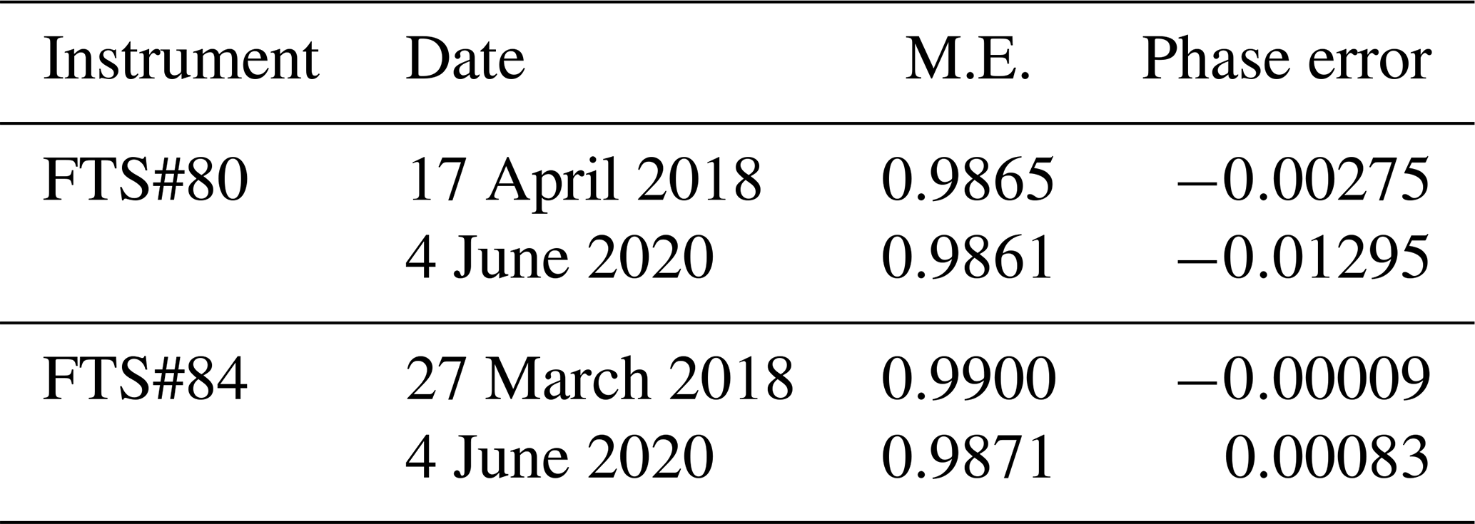
An important step to find any kind of instrumental malfunction is the laboratory calibration. Open-path measurements described by Frey et al. (2015) and Alberti et al. (2021) were performed for recognizing channelling effects, increased noise levels and out-of-band artefacts and for characterizing the instrumental line shape (ILS). The ILS for both instruments was determined at KIT before and after the campaign in order to track their stability and thus their performance. The ILS is given in terms of modulation efficiency (M.E.) and phase error (Table 1).
Table 1ILS in terms of modulation efficiency (M.E.) and phase error calculated before and after the campaign for instruments FTS#80 and FTS#84.
2.1.2 Side-by-side measurements
After the instruments were calibrated, solar side-by-side measurements between the instruments used in the campaign (FTS#80 and FTS#84), the COCCON reference and the TCCON spectrometer operated at the same location were carried out at KIT. These measurements served to find the instrument-specific calibration factors for each retrieved gas. These factors are calculated with respect to the COCCON reference and help to harmonize the results for all COCCON spectrometers. Such measurements took place before (18 and 19 April 2018) and during (12 April 2019) the campaign. The later one served for crosschecking whether the instruments kept the same behaviour and performance. These results can be seen in Figs. 1 and 2, respectively, and the correction factors are listed in Table 2.

Figure 1Side-by-side measurements before the instruments were shipped to Russia. Comparisons between instrument no. 1 (FTS#37), which is the COCCON reference unit operated at KIT, and instruments FTS#80 and FTS#84.
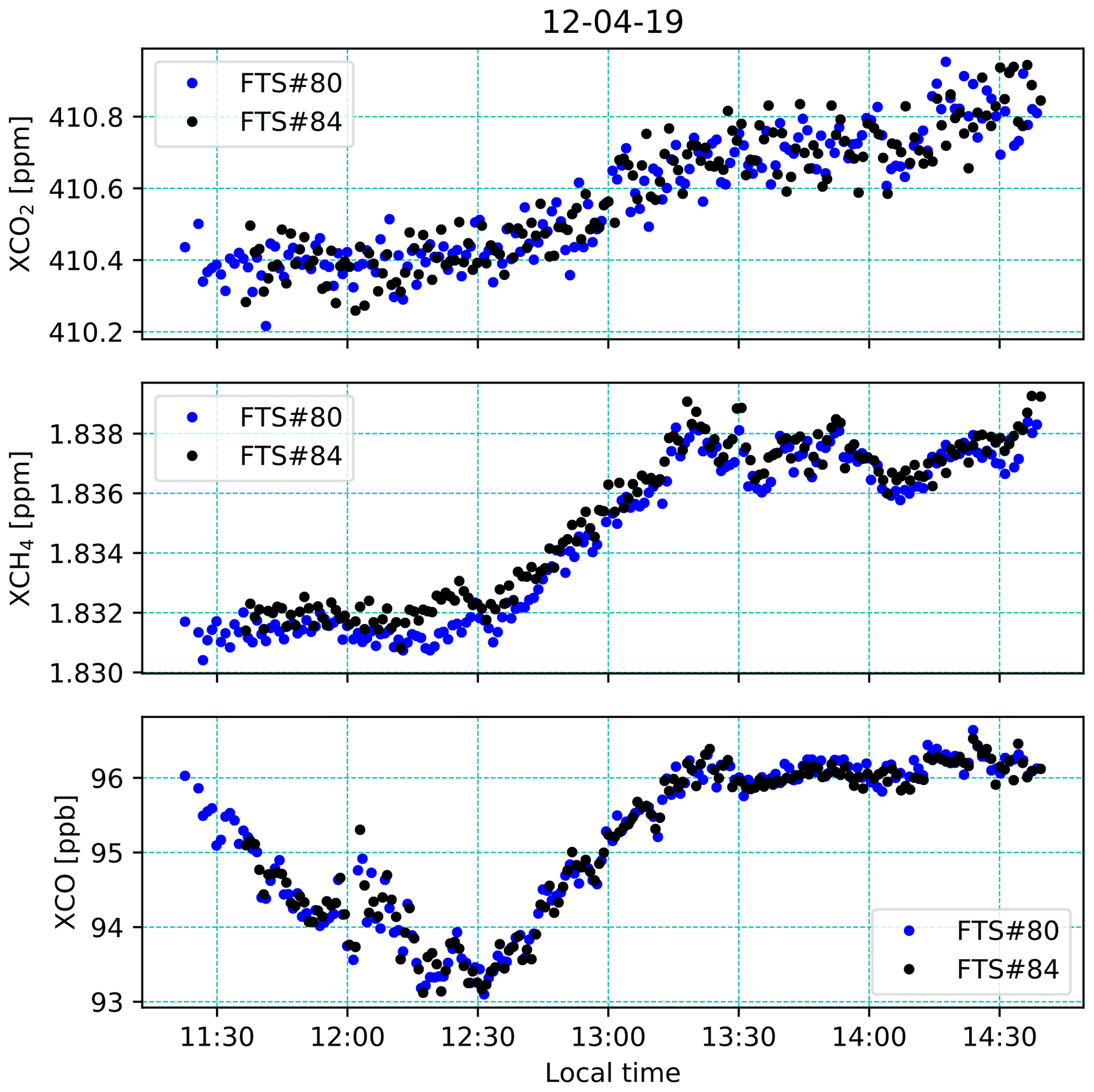
Figure 2Side-by-side measurements during the campaign but only with instruments FTS#80 and FTS#84.
Table 2Correction factors for instruments FTS#80 and FTS#84. The italicized values show the small drift of the instruments and the used values on the analysis.
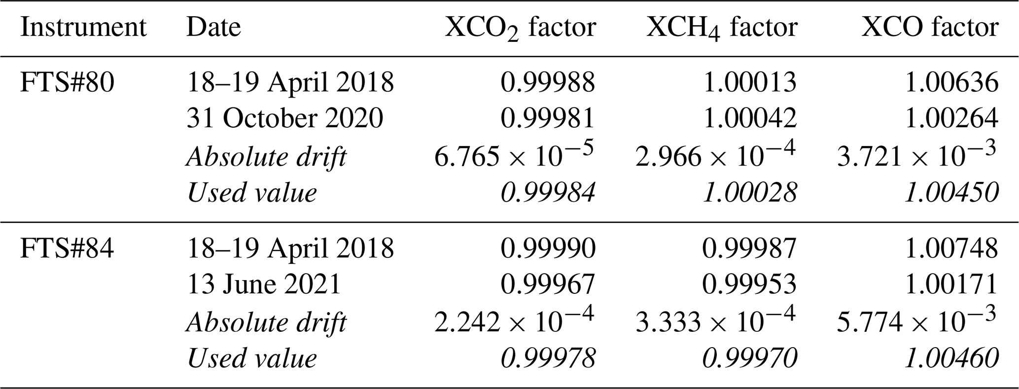
From the measurements shown in Fig. 1, the correction factors for XCO2, XCO and XCH4 measured by the two instruments are calculated as described in Frey et al. (2019) and Alberti et al. (2021). These results are averaged and later used for scaling the results for each of the retrieved GHGs analysed in this study as presented in Table 2.
2.2 EMME campaign
The EMME campaign is described in detail by Makarova et al. (2021), and here we summarize only the most relevant details of it. Because the aim of this campaign was to quantify the CO2 emissions; emission ratios; and the estimation of the CO2, CH4, and CO fluxes, two mobile COCCON FTIR spectrometers were used in order to retrieve the required GHG species. Both instruments were located in the upwind and downwind regions of the St Petersburg city ring. This campaign was not made in a continuous acquisition mode, but the active phases were scheduled according to the weather forecast. The basic idea is to select the deployment position of each instrument a day before good meteorological conditions appeared. The wind forecast, and the orientation of the city's NO2 plume as modelled by HYSPLIT (HYbrid Single-Particle Lagrangian Integrated Trajectory) (https://www.ready.noaa.gov/HYSPLIT_traj.php, last access: 4 August 2021) were used as prediction tools, and the positions of the COCCON spectrometers were selected accordingly. In addition, during a measuring day, the Russian partners carried out mobile zenith DOAS (differential optical absorption spectroscopy) measurements in order to measure the NO2 total column flux over the city in a near-real time manner. The second input helped to readjust the location of one or both spectrometers in case of deviations from the predicted plume orientation. Following this approach, a total of 11 successful measurement days were carried out during March to April 2019. An overview of the collected COCCON data is presented in Fig. 3; from that figure the enhancement on 25 April 2019 is remarkable. This measurement day is presented as a plume transport event in a city-scale domain tracked by TROPOMI as a complement of the results shown by Makarova et al. (2021).

Figure 3General overview of the full campaign results collected with the COCCON spectrometers (Makarova et al., 2021).
2.3 Ground-based FTIR measurements at Peterhof and Yekaterinburg
For the continuous, long-baseline campaign, the instrument FTS#80 remained at Peterhof station at the Saint Petersburg State University and continued operation there, while the other spectrometer (FTS#84) was moved to Yekaterinburg.
2.3.1 Peterhof (59.88∘ N, 29.83∘ E)
Peterhof is a suburb of St. Petersburg located approximately 35 km southwest from the city centre. The instrument in Peterhof was operated by the Russian partners at the Atmospheric Physics Department of the Faculty of Physics at Saint Petersburg State University. The instrument was set up on every sunny day (outside the city campaign period) at the second floor of the FTIR remote-sensing group (see Fig. 4). Eighty-four measurement days were collected between January 2019 and March 2020 as can be seen in Fig. 5. From that figure, the larger XCO observed values on 6 August 2019 in comparison to all the other days is remarkable. For more details, see Fig. A1a and b, where the spatial distribution of TROPOMI XCH4 and XCO, as well as wind speed and direction, respectively, for this day are presented. Additionally Fig. A1c shows the time series for COCCON XCO2, XCH4 and XCO for that day, and the enhancements are all observed in the three species. It seems that these large values could be related to a plume transport from a heavily industrialized area coming from Lappeenranta, which is located in the southeast of Finland and approximately 160 km away from Peterhof (see Fig. A2a). In order to confirm this, Fig. A2a shows the yearly CO emissions coming from the “Combustion from manufacturing sector” taken from the EDGAR V05 inventory (latest available: 2015), together with the backward trajectories calculated by using the HYSPLIT model and arrived in Peterhof on that day (see Fig. A2b). This confirms that the wind comes from the area where huge anthropogenic CO sources are located. Another possibility could be an even closer local source, like a small fire.
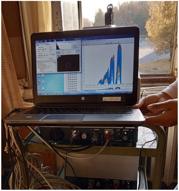
Figure 4Instrument set-up at Peterhof. A huge window allowed for measurements from ∼ 10:00 to ∼ 15:30 LT (local time) every day.
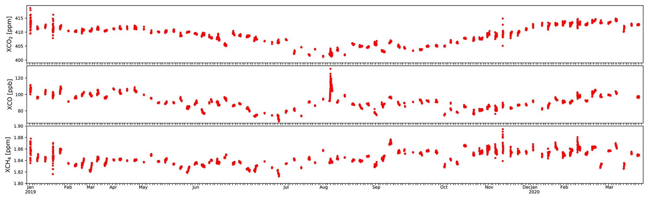
Figure 5Time series for XCO2, XCO and XCH4 obtained in Peterhof during the continuous campaign.
2.3.2 Yekaterinburg (56.8∘ N, 60.6∘ E)
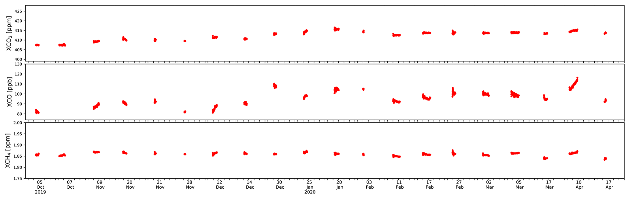
It was planned that immediately after the EMME campaign the instrument FTS#84 would be transported to Yekaterinburg. Unfortunately, unforeseen organizational problems significantly delayed moving the instrument from St. Petersburg to Yekaterinburg. The instrument was finally operational in Yekaterinburg in October 2019 and kept measuring until the very last day before being shipped back to KIT (April 2020). The instrument was operated at the Climate and Environmental Physics Laboratory INSMA of the Ural Federal University (UrFU). The instrument was set up in an internal yard of the UrFU building. However, the building structure, which blocked the sunlight, was a limitation. Sometimes high trucks passing through the yard blocked the field of view of the instrument (see Fig. 6). The spectrometer rested on the windowsill of the basement, so it was located exactly at ground level ∼260 m. Under good weather conditions, measurements were carried out approximately between 11:00 and 14:30 LT. In total, 22 d of measurements were collected as can be seen in Fig. 7.

Figure 6Instrument set-up at Yekaterinburg. The time interval of the daily measurements was constrained by the building structure, which blocked the sunlight.
In the following subsections, all the datasets used for this study are summarized, and a quick overview of them can be found in Table A1 in Appendix A.
3.1 Ground-based data
COCCON
Recently, COCCON (https://www.imk-asf.kit.edu/english/COCCON.php, last access: 13 May 2021; Frey et al., 2019) was established by continuous support granted by the European Space Agency (ESA). COCCON provides a supporting infrastructure for GHG measurements using the EM27/SUN spectrometer and ensures common standards for instrumental quality management and data analysis. The EM27/SUN spectrometer was developed by KIT in cooperation with the Bruker company in 2011 (Gisi et al., 2012). A second detector channel for XCO observations was added in 2015 (Hase et al., 2016). The EM27/SUN spectrometers are widely used, and there are currently about 78 instruments globally operated by different research groups. It has been shown in several studies that the results for these GHGs observed by COCCON instruments are in good agreement with official TCCON results (Frey et al., 2021; Sha et al., 2020). With the characteristics of compactness, robustness and portability, these instruments have been successfully used in several field campaigns and continuous deployments (Hase et al., 2015; Klappenbach et al., 2015; Chen et al., 2016; Butz et al., 2017; Sha et al., 2020; Vogel et al., 2019; Tu et al., 2020, 2021, 2022; Jacobs et al., 2020; Frey et al., 2021; Dietrich et al., 2021; Jones et al., 2021). A preprocessing tool and the PROFFAST non-linear least squares fitting algorithm are used for data retrieval. This processing software was created in the framework of the ESA COCCON-PROCEEDS and COCCON-PROCEEDS II projects. The solar zenith angle (SZA) range of COCCON data used in this study is restricted to ≤70∘ in order to limit uncertainties connected with spectra recorded at very high air masses.
3.2 Spaceborne data
3.2.1 TROPOMI
The Sentinel-5 Precursor (S5-P) satellite with the Tropospheric Monitoring Instrument (TROPOMI) on board as a single payload was launched in October 2017. S5-P is a low-Earth-orbit polar satellite. It aims at monitoring air quality, climate and ozone layer with high spatio-temporal resolution and daily global coverage during an operational lifespan of 7 years (Veefkind et al., 2012). TROPOMI is a nadir-viewing grating-based imaging spectrometer, measuring backscattered solar radiation spectra with an unprecedented resolution of 7×7 km2 (upgraded to 5.5×7 km2 in August 2019; Lorente et al., 2021b). In this study, we use the improved TROPOMI XCH4 product derived with the RemoTeC full-physics algorithm (Lorente et al., 2021b) and apply the recommended quality value (qa) =1.0 to the data. For CO, SICOR (Shortwave Infrared CO Retrieval algorithm) is deployed to retrieve the total column density of CO from TROPOMI spectra at 2.3 µm (Landgraf et al., 2016; Borsdorff et al., 2018a, b). XCO is computed by dividing the CO total column by the dry air column extracted from the co-located TROPOMI CH4 file. This dry air column is obtained from the surface pressure and water vapour column as provided by the European Centre for Medium-Range Weather Forecasts (ECMWF) analysis (Schneising et al., 2019; Lorente et al., 2021b). H2O retrievals are also performed with the SICOR algorithm. A similar quality filter is applied to the H2O product as used in Schneider et al. (2020).
3.2.2 OCO-2
The Orbiting Carbon Observatory-2 (OCO-2) is a NASA satellite, launched in July 2014, providing space-based measurements of atmospheric CO2 (Eldering et al., 2017). These observations have the potential capability to detect CO2 sources and sinks with unprecedented spatial and temporal coverage and resolution (Crisp, 2015). The OCO-2 mission carries a single instrument incorporated with three high-resolution imaging grating spectrometers, collecting spectra from reflected sunlight by the surface of Earth in the molecular oxygen (O2) A band at 0.764 µm and two CO2 bands at 1.61 and 2.06 µm (Osterman et al., 2020). The OCO-2 satellite has three viewing modes (nadir, glint and target) and a near-repeat cycle of 16 d (98.8 min per orbit, 233 orbits in total). It samples at a local time of about 13:30 LT. The current version (V10r) of the OCO-2 Level 2 (L2) data product, containing bias-corrected XCO2, is used in this study.
In addition to the operational XCO2 product derived from OCO-2 observations described above, the data product generated using the Fast atmOspheric traCe gAs retrievaL (FOCAL) algorithm described in Reuter et al. (2017a, b) had been used. Compared with co-located TCCON observations, the OCO-2 FOCAL data show a regional-scale bias of about 0.6 ppm and single measurement precision of 1.5 ppm (Reuter and Buchwitz, 2021). In this study, the latest version (v09) covering the time period of 2015–2020 is utilized for further comparison with the COCCON results.
3.2.3 MUSICA IASI
The Infrared Atmospheric Sounding Interferometer (IASI) is a payload on board the EMETSAT Metop series of polar-orbiting satellites (Clerbaux et al., 2009). The IASI instrument is a Fourier transform spectrometer that measures infrared radiation emitted from the Earth and emitted and absorbed by the atmosphere. It provides unprecedented accuracy and resolution on atmospheric humidity profile, as well as total column-integrated CO, CH4 and other compounds twice a day. There are currently three IASI instruments in operation on Metop-A, Metop-B and Metop-C, launched in 2006, 2012 and 2018, respectively. The MUSICA IASI retrievals are based on a nadir version of PROFFIT (Schneider and Hase, 2009), which has been developed in support of the MUSICA project. More details can be found in Schneider and Hase (2011) and Schneider et al. (2022). A validation of the MUSICA IASI H2O profile data is presented by Borger et al. (2018).
3.2.4 GOSAT
The Greenhouse Gases Observing Satellite (GOSAT) was launched in January 2009, equipped with two instruments (the Thermal And Near-infrared Sensor for carbon Observation Fourier Transform Spectrometer, TANSO-FTS, and the TANSO Cloud and Aerosol Imager, TANSO-CAI) (Kuze et al., 2009). The satellite is placed on a Sun-synchronous orbit and passes the same point on Earth every 3 d. GOSAT is the first mission to monitor the global distribution and sinks and sources of GHGs. For this study, GOSAT FTS shortwave infrared (SWIR) level-2 data, version V02.90, from the National Institute for Environmental Studies (NIES) are used.
3.3 CAMS data
3.3.1 CAMS inversion
Copernicus Atmosphere Monitoring Service (CAMS) is operated by the European Centre for Medium-Range Weather Forecasts (ECMWF), providing global inversion-optimized GHG concentration products which are updated once or twice per year. For XCO2 and XCH4, the latest version datasets (v20r1 for XCO2 and v19r1 for XCH4) using surface air-sample as observations input are used in this study. The CAMS global CO2 atmospheric inversion product is generated by the inversion system, called PyVAR (Python VARiational), with a horizontal resolution of and temporal resolution of 3 h (Chevallier, 2020a, b). The latest version (V20r1) was released in December 2020, covering the period from January 1979 to May 2020. The V20r1 model data fit TCCON retrievals well with less than 1 ppm of absolute biases (Chevallier, 2020b).
For XCH4, we used the latest version V19r1 based on inversion of surface observations only, covering the period between January 1990 and December 2019. The CAMS XCH4 inversion product is based on the TM5-4DVAR (four-dimensional variational) inverse modelling system (Bergamaschi et al., 2010, 2013; Meirink et al., 2008) with a horizontal resolution of and temporal resolution of 6 h (Segers, 2020a, b). Compared to previous releases, v19r1 data have been adjusted by using new atmospheric CH4 sinks and updated wetland emissions, and the monthly bias is usually less than 10 ppb with respect to TCCON (Segers, 2020b).
3.3.2 CAMS reanalysis (control run)
This study aims to compare XCO retrieved from the COCCON measurements with XCO from different satellite and CAMS datasets as well. However, no XCO data are available from the before-mentioned CAMS data. Fortunately, CAMS also provides reanalysis datasets, covering the period of 2003–June 2020. The standard CAMS reanalysis data use 4DVar data assimilation in CY42R1 of ECMWF's Integrated Forecast System (IFS) (Flemming et al., 2017; Inness et al., 2019). The CAMS reanalysis CO profiles under a control run, i.e. without any data assimilation, is obtained from Copernicus Support team. This control run reanalysis CO profiles are using only one IFS cycle with a latitude × longitude resolution, 3 h of temporal resolution and 25 pressure levels. XCO is obtained when integrating the profiles from the lowest to the highest pressure level.
4.1 Seasonal variability of GHGs
4.1.1 Peterhof
The seasonal patterns of the retrieved GHGs are shown in Fig. 8, which illustrates the time series of daily mean XCO2, XCH4, XCO and XH2O from different data products at Peterhof. The CAMS-COCCON data product presented in Figs. 8 and 9 is discussed in Sect. 4.3. The TROPOMI satellite has a higher spatial resolution and therefore, the available retrieved species from TROPOMI were daily averaged within a collection radius of 50 km around Peterhof. For the GOSAT and MUSICA IASI datasets, a collection radius of 100 km around Peterhof is used, and for OCO-2 data, a collection radius of 200 km is used. The choice of collecting radius is considered based on the available satellite observations and the bias between a single satellite observation and the coincident COCCON observation (see Fig. A3). The measurements from the different ground- and space-based observations and model data generally show good agreements and similar seasonal variability.
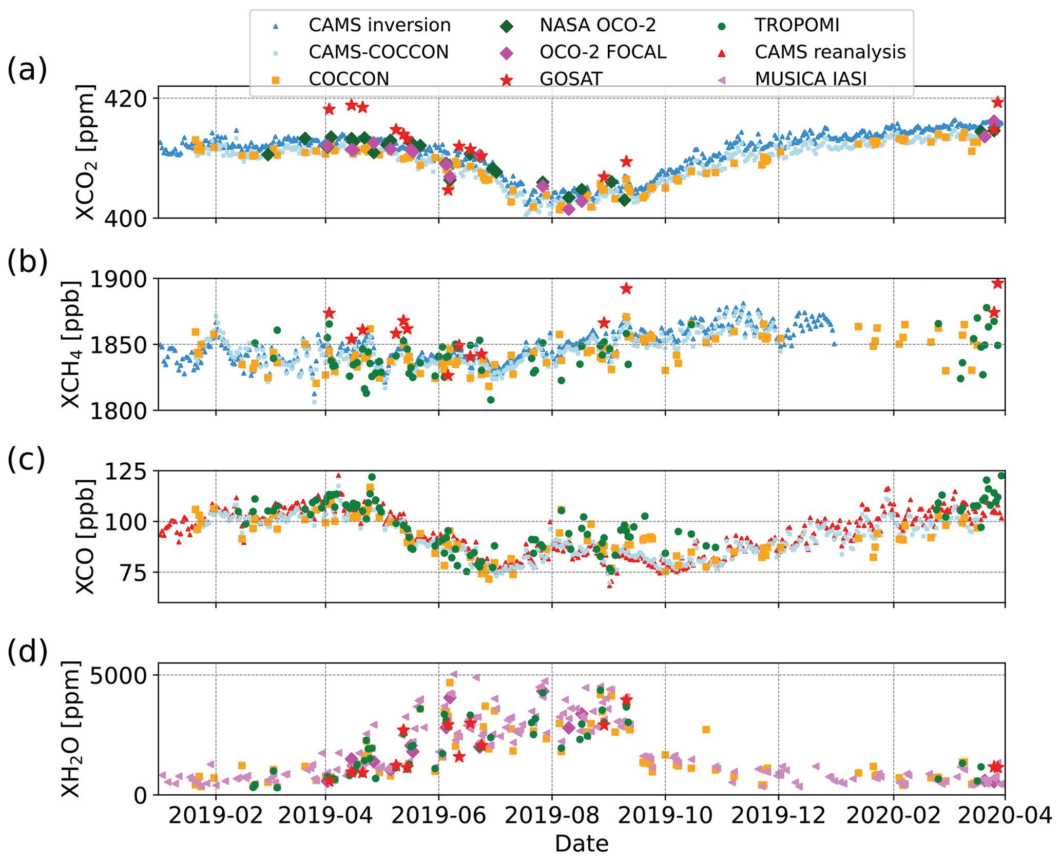
Figure 8Time series of daily mean (a) XCO2, (b) XCH4, (c) XCO and (d) XH2O for different data products at Peterhof.
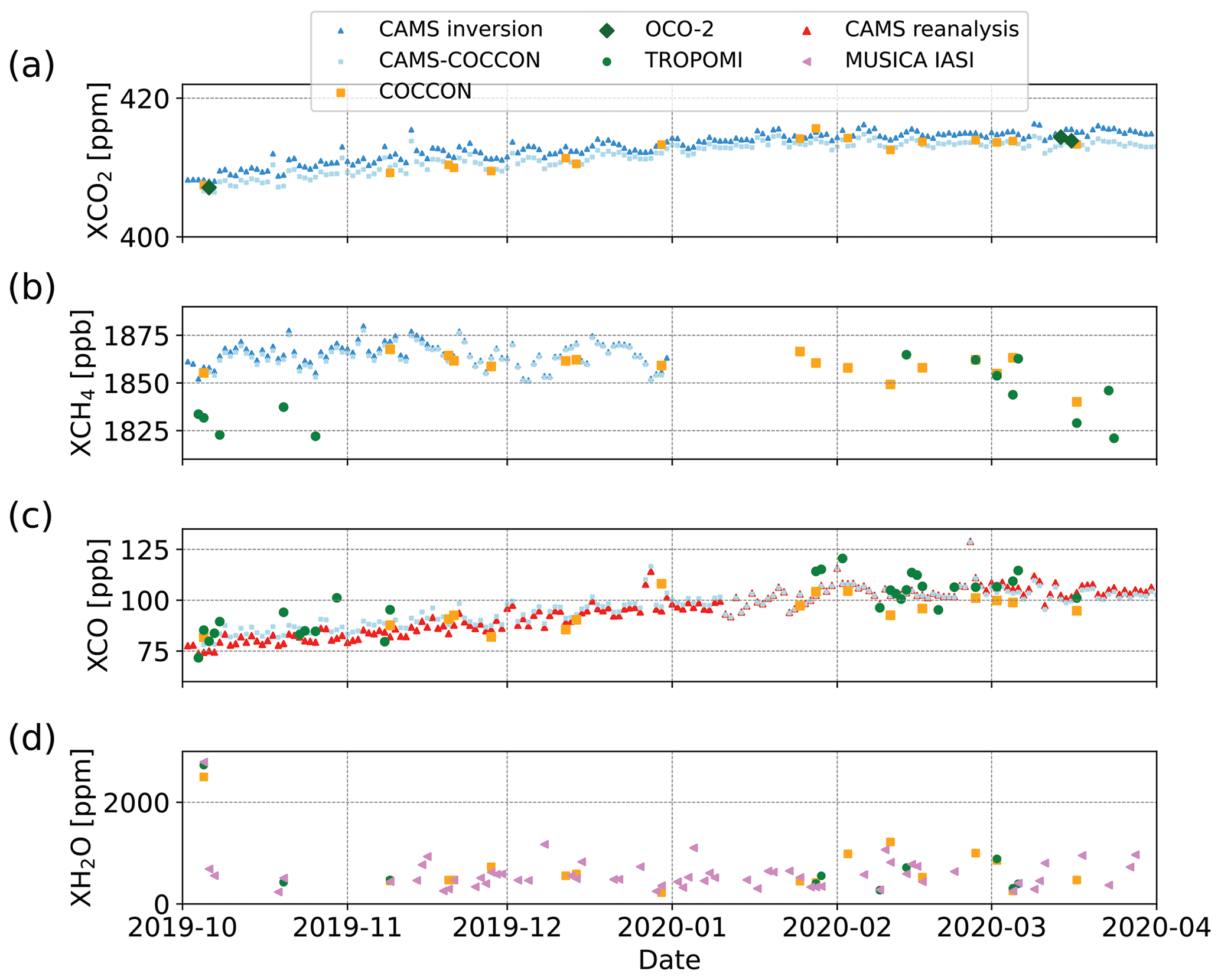
Figure 9Time series of daily mean (a) XCO2, (b) XCH4, (c) XCO and (d) XH2O for different data products at Yekaterinburg.
CAMS and the satellite products show a high bias of about 0.81 to −3.1 with respect to COCCON. GOSAT (Fig. 8a) also shows some obvious outliers compared to the other products, which have similar behaviours. The amount of XCO2 varies along the year, and much of this variation is driven by respiration, which never stops but increases between autumn and winter due to reduced uptake (no photosynthesis). In this case the atmospheric XCO2 concentration is stable between January and April. It started to decrease from May to end of July, during which the growing season and the photosynthetic activities increase. Similar behaviour in 2019 was also observed by Timofeyev et al. (2021) and in previous years by Timofeyev et al. (2019) and Nikitenko et al. (2020). The amount of XCO2 stays around 403 ppm between the end of July and middle of September and starts to increase afterwards.
For XCH4, COCCON shows a similar behaviour as TROPOMI and CAMS. Slightly higher mean values and variability can be seen in GOSAT XCH4 with a few outliers. Compared to XCO2, XCH4 shows generally less seasonal variabilities with more short-term enhancements of about a week duration, probably related to synoptic variations. The seasonal variation is comparable to the results of Gavrilov et al. (2014), Makarova et al. (2015a, b) and Timofeyev et al. (2016). A slightly higher XCH4 is observed at the end of 2019 for all data products.
XCO shows seasonal variability with a maximal value of 110 ppb in late April and decreases by nearly 40 % to 70 ppb in the beginning of July. A secondary local maximal reaching ∼95 ppb occurs in August. This feature needs further investigation. The COCCON XCO matches well to the CAMS reanalysis data. Moreover, COCCON agrees better with the TROPOMI data in summer than in spring and late autumn, when TROPOMI measured higher values.
XH2O shows a strong seasonal cycle with a maximal amount of ∼4700 ppm in summer and minimal amount of ∼320 ppm in winter. All products show quite similar behaviour with high variability, which is similar to those in Semenov et al. (2015), Timofeyev et al. (2016) and Virolainen et al. (2016, 2017). The GOSAT data have higher mean values since the measurement period covers only the time range from later spring to summer, during which higher XH2O is observed.
4.1.2 Yekaterinburg
The measurement period covered winter and spring, from 5 October 2019 to 17 April 2020 at Yekaterinburg (Fig. 9). Here we use a larger radius (100 km) to collect the TROPOMI observations, because there are much fewer overpasses at Yekaterinburg during this period. Table A2 in Appendix A lists the number of coincidences (pixel-wise) for 50 and 100 km radius, and the number of coincident satellite pixels is reduced by a factor of 3 to 5 for the narrower radius. From Fig. A4 in Appendix A, we do see a tendency of slightly reduced differences with better co-location within the 100 km limit in case of XCH4 but not clearly for the other species. Due to the low number of coincident measurements when using 50 km, we decided to accept the 100 km distance criterion for the Yekaterinburg observations.
XCO2 shows a clearly increasing tendency from October of 408 ppm to a maximal value of 415 ppm in the middle of February, which covers later autumn and winter. This is because on top of the increase due to the anthropogenic emissions there are variations due to photosynthesis and respiration (https://atmosphere.copernicus.eu/carbon-dioxide-levels-are-rising-it-really-simple, last access: 2 July 2021). During that period the plants notably reduce or stop the photosynthesis processes which could increase the amount of CO2 in the atmosphere. Later this maximal value stays constant until the middle of March. It tends to decrease, and a similar behaviour is observed in Peterhof.
For XCH4, COCCON shows a good agreement with CAMS data, though there are not so many COCCON observations. XCH4 shows generally decreasing tendency but with more short-term variabilities. Such variabilities are observed in Peterhof as well. A few TROPOMI observations in October are deviating from the other two datasets, and it seems that TROPOMI underestimates XCH4. This might be because most TROPOMI measurements are located in the rim of the collecting radius and thus away from the location of Yekaterinburg, introducing some errors (see Fig. A5). Further, this underestimation could be due to the difficulty for retrieving CH4 in low- and high-albedo scenes (Lorente et al., 2021b).
XCO shows in general a similar behaviour of XCO2, with a steady increase during late autumn and winter. It seems that the increasing behaviour of XCO has an inverse relationship with XCH4. This is probably due to the fact that atmospheric CO is mainly produced by incomplete combustion of fossil fuels (Kasischke and Bruhwiler, 2002) and the oxidation of methane (Cullis and Willatt, 1983).
As expected, most XH2O values are below 1000 ppm, similar to Peterhof in that period. This can be explained by the saturation concentration of water vapour in air, which reduces for lower temperatures.
4.2 Removal of the smoothing error bias
Because we aim at comparing different data products (such as spaceborne and COCCON products) and each of them use different sensitivities and different a priori profiles, it is important to account for these differences when comparing a defined Xgas species as described by Rodgers and Connor (2003) and Connor et al. (2008). Such procedures have been applied in similar studies (Hedelius et al., 2016; Yang et al., 2020; Sha et al., 2021). In this study, we used the method described in Connor et al. (2008). We took as starting point their Eq. (13); then the state vector can be written as
where VMR represents the volume mixing ratio. The left-hand term of the equation represent the retrieved value, while the right-hand term represents the VMR calculated based on the a priori profiles plus the effect of the averaging kernel matrix A applied to the difference of the VMR between the true atmospheric gas concentration and the a priori profiles. By dividing the atmosphere into k layers, this equation can be written as follows:
where with y being a defined a priori profile used and hk being the pressure-weighting function in a defined layer k (Connor et al., 2008), i.e.
By using Eq. (2) with “new” and “old” satellite a priori profiles, we obtain (*) and as follows:
Then we subtract (*) from :
which turns into
where in Eq. (4) becomes the smoothed satellite product, which takes into account the a priori profiles used for the COCCON retrievals.
When using Eq. (4), both a priori profiles need to be resampled on the same pressure grid. The vertical profiles used for the COCCON analysis are interpolated to the pressure levels of different satellite products (TROPOMI CO, GOSAT CO2 and CH4, OCO-2 CO2, and OCO-2 FOCAL CO2) by using the mass conservation method described in Langerock et al. (2015).
The smoothing correction is not applied to XH2O, because the natural variability of XH2O is very high anyway.
4.3 Correlation between COCCON and satellite products
All satellite XCO2, XCH4 and XCO data used in this section were adjusted for the COCCON a priori profile (TCCON a priori profiles were used) as described above. In addition, in the Supplement of this paper, the comparisons with the original COCCON products (see Figs. S1 to S4 in the Supplement) and without taking into account the averaging kernels when comparing with satellite products are presented.
Figures 10 to 13 show the correlations between COCCON and different satellite products at Peterhof (triangle symbols) and at Yekaterinburg (dot symbols). The satellite products and CAMS generally agree well with COCCON. Figure 14 illustrates the averaged bias and standard deviation of each product of the coincident Xgas (XCO2, XCH4 and XCO) values (in space-time) with respect to COCCON for the available gases at both sites. In order to find the coincident COCCON data, the mean value of the observations 2 h before and after a centralized time reference is taken. Such a time reference differs for each of the products as follows: the overpass time for satellite and each of the timestamps for CAMS.

Figure 10Correlation plots between TROPOMI and COCCON for XCH4, XCO and XH2O at Peterhof (a–c) and at Yekaterinburg (d–f). All satellite data except XH2O were adjusted for the COCCON a priori profile (TCCON a priori profiles were used).

Figure 11Correlation plots (a–b) between NASA's operational and the FOCAL OCO-2 product and COCCON for XCO2 and (c) between OCO-2 FOCAL and COCCON for XH2O at Peterhof. All satellite data except XH2O were adjusted for the COCCON a priori profile (TCCON a priori profiles were used).
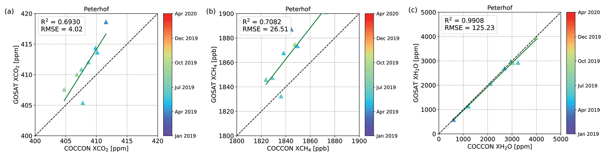
Figure 12Correlation plots between GOSAT and COCCON for (a) XCH4, (b) XCO and (c) XH2O at Peterhof. All satellite data except XH2O were adjusted for the COCCON a priori profile (TCCON a priori profiles were used).

Figure 13Correlation plots of XH2O between MUSICA IASI and COCCON at (a) Peterhof and (b) Yekaterinburg.
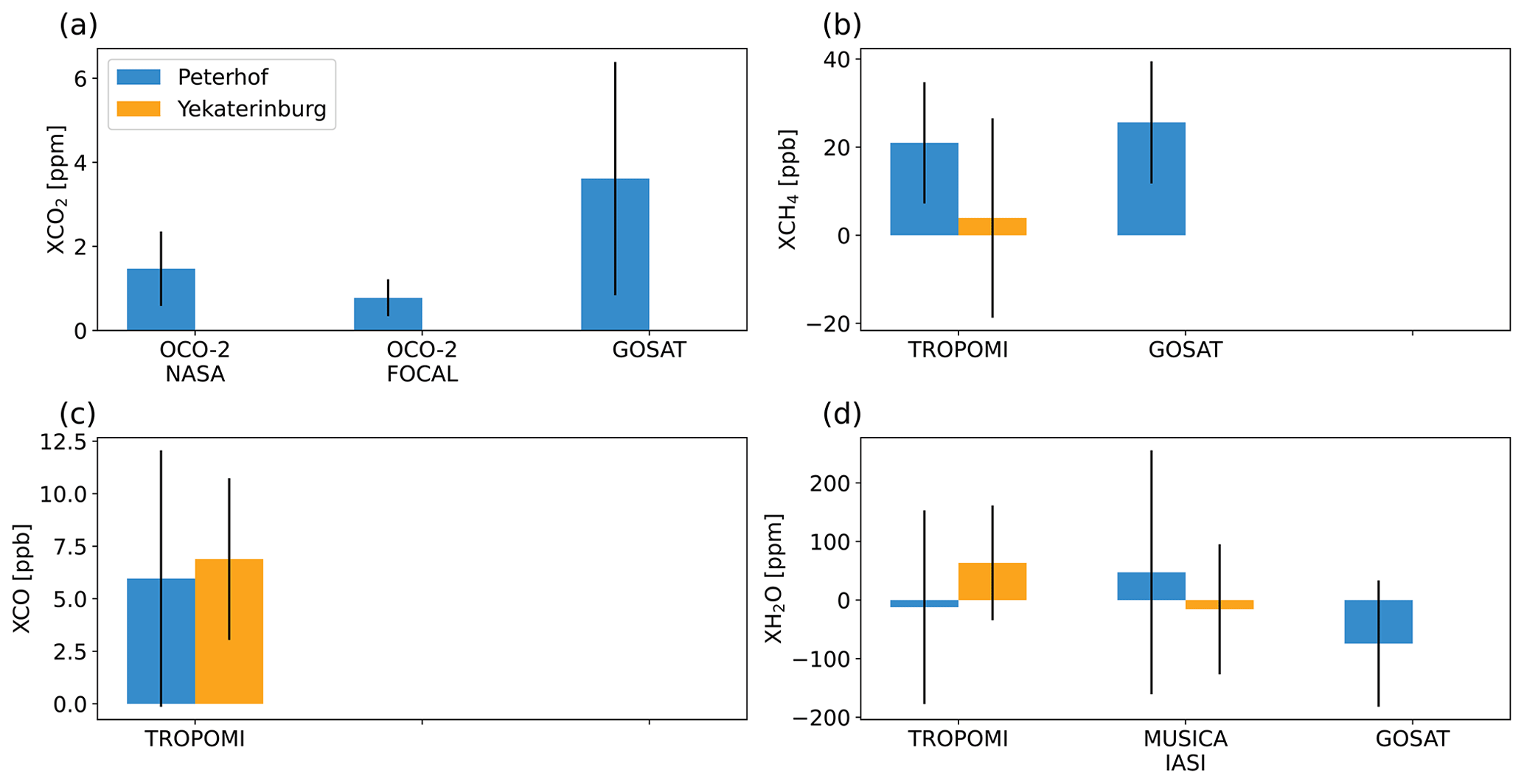
Figure 14Bar plots of the averaged bias derived from different products with respect to COCCON for (a) XCO2, (b) XCH4, (c) XCO and (d) XH2O at Peterhof and Yekaterinburg. The error bars represent the standard deviation of the averaged bias.
The measuring period at Yekaterinburg for COCCON was mostly in winter and early spring, from October 2019 to April 2020, in which there were fewer sunny days. This results in fewer COCCON and satellite observations. There is only one coincident point between COCCON and NASA operational OCO-2 (Fig. 11c) and no coincident points between COCCON and OCO-2 FOCAL or GOSAT products at Yekaterinburg. Even a much larger collection circle with a radius of 100 km is used for TROPOMI at Yekaterinburg, and there are fewer coincidence measurements than those in Peterhof, where more than 1 year of measurements were performed.
Due to the short period of ground-based measurements, poor weather condition, and poorer coverage of satellites at high latitudes in the winter hemisphere (OCO-2; Patra et al., 2017, and GOSAT; https://data2.gosat.nies.go.jp/gallery/fts_l2_swir_co2_gallery_en.html, last access: 28 June, 2021), it becomes more difficult to validate satellite products with ground-based measurements at locations like Yekaterinburg.
At Peterhof OCO-2 FOCAL XCO2 data have the lowest bias with respect to COCCON, while GOSAT data show the highest bias and standard deviation (3.6 ppm ± 2.8 ppm, Fig. 14). NASA operational OCO-2 and CAMS show similar biases. CAMS, TROPOMI and GOSAT measure higher XCH4 than COCCON, among which GOSAT has the highest biases at Peterhof. The high negative bias in TROPOMI at Yekaterinburg is mainly due to the underestimation of the TROPOMI product in October 2019. At both sites TROPOMI XCO shows higher biases than CAMS with respect to COCCON, which can be seen in Figs. 8c and 9c – TROPOMI with higher values than COCCON. TROPOMI and GOSAT generally measure lower XH2O than COCCON, whereas MUSICA IASI shows high bias and standard deviation. However, good correlations can be found between satellite XH2O and COCCON in Figs. 10c, f, 12c and 13.
4.4 Using CAMS model fields for upscaling COCCON observations
Unfortunately, during the continuous campaign carried out at Peterhof and Yekaterinburg, there are just a few coincident measurement days with satellite observations, especially in comparison to GOSAT and OCO-2 (see Fig. 14). Although these satellites offer a global coverage, for our measurement period (even with quite relaxed coincidence criteria), the comparisons do not use the majority of the ground-based observations. This is especially the case in Yekaterinburg during the observations from October 2019 to April 2020, i.e. GOSAT and OCO-2 have none or just a couple of measurements in the winter and early spring period at high latitudes. Even in Peterhof where more than 1 year of measurements were taken, the number of coincident measurements between the aforementioned satellites is rather few.
For that reason, we employ a novel method which uses model fields for upscaling the ground-based FTIR measurements, thereby generating additional virtual coincidences. Such upscaling does not use one global scaling factor but a time-resolved one, as shown in Figs. A6, A7 and A8 in Appendix A. Although some noise is superimposed on the temporal evolution of scaling factors, a seasonal cycle becomes apparent.
In a first step, CAMS model data are adjusted to match the value for COCCON. Then, the adjusted model fields are compared with the available satellite results data for XCO2, XCH4 and XCO. The assumption of this method is that the bias of the model field is a smooth function in space and time, which seems well justified due to the long atmospheric lifetime of the gases under consideration. Since the model considers all relevant aspects of dynamics (advection, changes in tropopause altitude) and attempts to even reproduce abundance changes due to sources and sinks, we expect that our approach is superior to ad hoc schemes typically used for enlarging the co-location area (e.g. using the potential temperature; see Keppel-Aleks et al., 2011). In order to avoid circular reasoning in the validation based on the adjusted model fields, the method should avoid model simulations which include the assimilation of satellite data.
4.4.1 Generation of the CAMS fields adjusted to COCCON observations
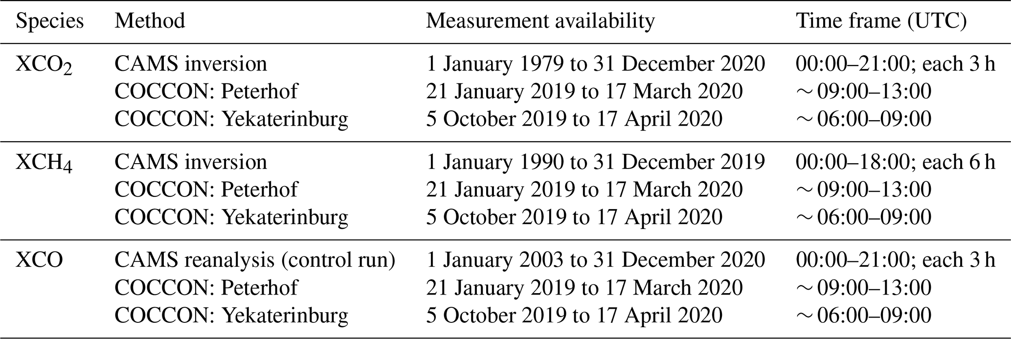
CAMS inversion results with surface air-sampled observations as input have been used for XCO2 and XCH4 (Segers, 2020a). Unfortunately, no XCO data are available on that model run. No XCO product from CAMS limits us from comparing one of the main data products of S5-P (XCO), which offers a greater number of measurements with a high horizontal resolution in comparison to any other satellite. Instead, the CAMS team has provided special profiles of CO from CAMS reanalysis data (control run). On that run, two important points have to be mentioned: (1) no total columns for CO2 and CH4 were available from this special dataset, and (2) no satellite data have been assimilated. Such results are available on a daily basis as described in Table 3. CAMS inversion is available on a daily basis for XCO2 and XCH4 but with different time frames. Unfortunately, there are no XCH4 results from CAMS for 2020, which adds a new constraint when simply comparing both results, especially for Yekaterinburg where approximately 4 out of 6 months were measured in 2020.
Table 3Time range and usual daily time frame of the analysed results from CAMS and COCCON.
As explained before, the main idea is to adjust XCO2, XCH4 and XCO from CAMS by using COCCON results. This is achieved by performing a time-resolved scaling of the model data, which is informed by the available ground-based observations. The detailed workflow encompasses the following steps, which are represented in Fig. 15.
-
As shown in Table 3, CAMS XCO2 and XCH4 are available on a daily basis in different prescribed time frames, while COCCON results are only available when specific conditions were fulfilled: good weather conditions (sunny or almost sunny conditions), no mobile campaign or manpower available to start the measurements, because the instruments were manually operated. These conditions made the measurements rather sparse, but nevertheless there still is a significant number of measurements available. Therefore, the first step is to find the coincident days between CAMS and COCCON and then the COCCON results are averaged around each CAMS time if available. As the COCCON observations require sunlight, all CAMS points before 06:00 UTC and later than 18:00 UTC were filtered out. For the aforementioned, each averaged CAMS time was considered reference, and all the COCCON results ±2 h were averaged as the coincident data. After these steps, we have both results on the same time gridding.
-
The outputs from the first step are time series with coincident measurement days and time frames. These time series, which have the same date boundaries, are then divided into n smaller intervals or sub-windows. These sub-windows have the characteristics of being non-overlapping, and they form equally sized bins on the time axis, as defined in the Eq. (5), where “DT” stands for “Date–Time”, which goes from the first to the last point of the measurement period. The user only needs to define the number of sub-windows n.
-
Additionally, a sliding sub-window, with the same size described in step 2, is run over both time series with the main difference being shifted by half of the size of the initial sub-window but still being not overlapping between them. Therefore, after step 2, step 3 is done in order to look at the neighbours.
-
In each of these sub-windows (described above, steps 2 and 3), a correlation analysis is carried out independently of the other sub-windows. In order to make the COCCON time series adjust better to CAMS results, a linear correlation with the intercept forced to zero is carried out; therefore, the slope gives the scaling factor for the CAMS data.
-
Each sub-window defined in step 2 is taken as a base with its slope calculated in step 4. After that, the slopes in the neighbourhood are also calculated in each overlapping sub-window defined in step 3, Finally, all the slopes are then averaged. Such averaged slope represents the scaling factor in that sub-window. It is important to mention that this number of sub-windows (and then its size) was adjusted until good results were achieved as described below.
-
Finally, with the scaling factor calculated in step 5, the original CAMS fields keeping their original temporal sampling are scaled in the whole range of each sub-window.
4.4.2 Selection criteria for the best number of windows
In order to choose the best number of windows, the scaling code is run starting from windows =1 and stops when two different conditions are fulfilled:
-
The root-mean-square deviation (RMSD), which is calculated with the Eq. (6), where k stands for the number of points considered during the scaling in each sub-window, between COCCON and the CAMS-COCCON data, must be the lowest possible.
-
The number of measurement points in each of the windows must be larger than four.
The second condition is very important, because if the number of windows increases, the window size (number of measurement points) decreases until no more points are available in some windows as the distribution of measurement points in the time domain is non-homogeneous.
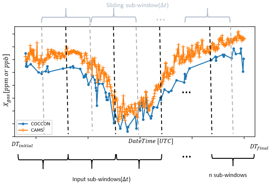
Figure 15Principle of the scaling method. Sub-windows are separated with black dotted lines and sliding sub-windows with grey dotted lines. The window size (Δt) is defined in Eq. (5).
4.4.3 Verification of the method
In order to test the method before it is applied to the study area, a much denser dataset in COCCON is used to prove its performance. Two years of measurements (January 2018–December 2020) taken in Karlsruhe with the instrument FTS#37, which is the reference in COCCON, were selected for this purpose. For the sensitivity study, three different subsets were generated from the original dataset. Such subsets consist of a percentage (40 %, 60 % and 80 %) of the total amount of measurement days, which are randomly selected. This is done in order to simulate the reduced number of observations available in the study area. The GHG used for this short sensitivity study is XCH4, because a comparison between each of the scaling results (for each dataset) can be compared with TROPOMI as well. The main results of this verification exercise are presented in Figs. A9 to A11 in Appendix A. In Fig. A9, a plot showing RMSD as a function of the number of windows is presented for each subset. Such results are used in order to decide the best number of windows. The correlations between CAMS and the original COCCON XCH4 measurements are presented in Fig. A10a, whereas Fig. A10b, c and d show the results between COCCON XCH4 and its CAMS-COCCON for 40 %, 60 % and 80 % of the original COCCON data, respectively. The satellite comparisons of the original COCCON XCH4 with TROPOMI are shown in Fig. A11a, whilst Fig. A11b, c and d show the TROPOMI XCH4 comparison but for CAMS-COCCON by using 40 %, 60 % and 80 % of the original COCCON measurement days. The most important conclusion can be drawn from Figs. A11 and A6. Figure A11 indicates a small bias between CAMS and COCCON (of about 0.12 %), which is successfully removed in the CAMS-COCCON fields, so the latter data approximate the missing observational value in an optimal sense. Figure A6 shows the scaling factor as a function of time, clarifying that the correction is not just the trivial removal of a constant bias factor but that some seasonal variation in the model – observation difference can be corrected as well. Note that we do not require in our approach that the COCCON values are superior over the CAMS values. This test is performed to clarify that the CAMS fields adjusted in the manner we described before provide the best prediction for what COCCON would have observed on a certain date.
4.5 Combined data results by using the scaling method
In order to generate the CAMS-COCCON product, we reprocessed the COCCON observations with the CAMS-Xgas a priori data. Additionally, in Figs. S6–S10, the comparisons with the original CAMS-COCCON, generated by using TCCON a priori data and without taking into account the smoothing error when comparing with satellite products, and a summary table are presented (see Table S1 in the Supplement).
The scaling method described above is applied to XCO2, XCH4 and XCO at Peterhof and Yekaterinburg. The numbers of selected windows for XCO2, XCH4, and XCO were 11, 10, and 11 at Peterhof and 5, 2, and 4 at Yekaterinburg, respectively. These scaled results are then compared with all the available satellite products as described in this study.
In order to correctly compare each of the satellite products to the CAMS-COCCON ones, the a priori profiles of the satellite retrievals were adjusted (replacing the original a priori profile by CAMS profiles) using the method described in Sect. 4.2.
4.5.1 Peterhof
After using the scaling method, the COCCON-adjusted CAMS data show close agreement with COCCON for XCO2, XCH4 and XCO (see Fig. A12 and Table A3). From Table A3 in Appendix A, it can be observed that the bias and the standard deviation between scaled CAMS and COCCON is significantly smaller than the CAMS variability of the original dataset. This further demonstrates the “close agreement” between adjusted model and observation.
The CAMS-COCCON data fill the gap during the measurements, providing a continuous period of a new intermediate or combined (CAMS-COCCON) data product, which helps to have more coincident data with satellite observations. Figures 16 to 18 show the CAMS-COCCON data in comparison to the available observations from different satellite products. There are more coincident data points for the operational OCO-2 product than OCO-2 FOCAL XCO2, which could be because the OCO-2 product has approximately 3 times more soundings (https://climate.esa.int/sites/default/files/ATBDv1_OCO2_FOCAL.pdf, last access: 2 July 2021). However, their correlations and patterns are quite similar, whereas OCO-2 FOCAL shows better agreement with CAMS-COCCON data. GOSAT XCO2 has a similar correlation with CAMS-COCCON as found for OCO-2 data but with some outliers. For XCH4, the CAMS-COCCON data are mostly higher than TROPOMI but lower than GOSAT, and this shows a good agreement with GOSAT with R2∼0.7, contrary to TROPOMI where R2∼0.12. The CAMS-COCCON XCO agrees well with TROPOMI data with an R2∼0.7.
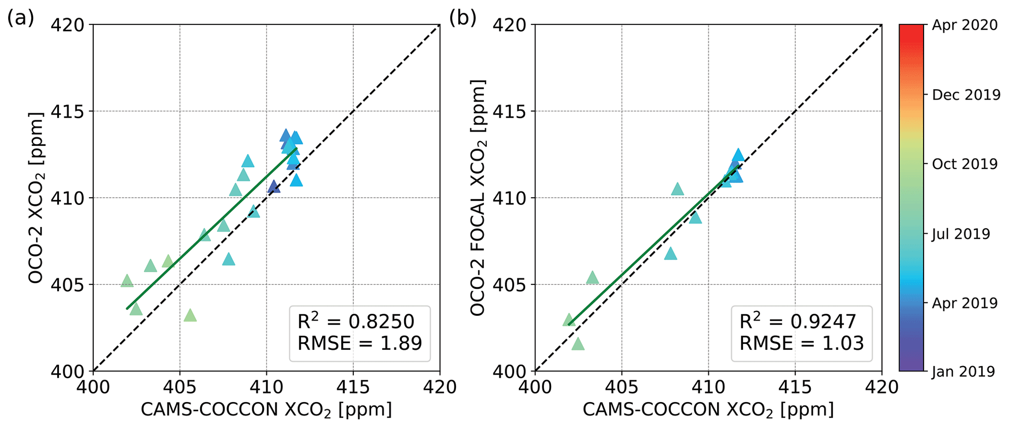
Figure 16Correlation plots of (a) OCO-2 and (b) OCO-2 FOCAL with respect to CAMS-COCCON XCO2 at Peterhof. All satellite data were adjusted for the CAMS a priori profile.
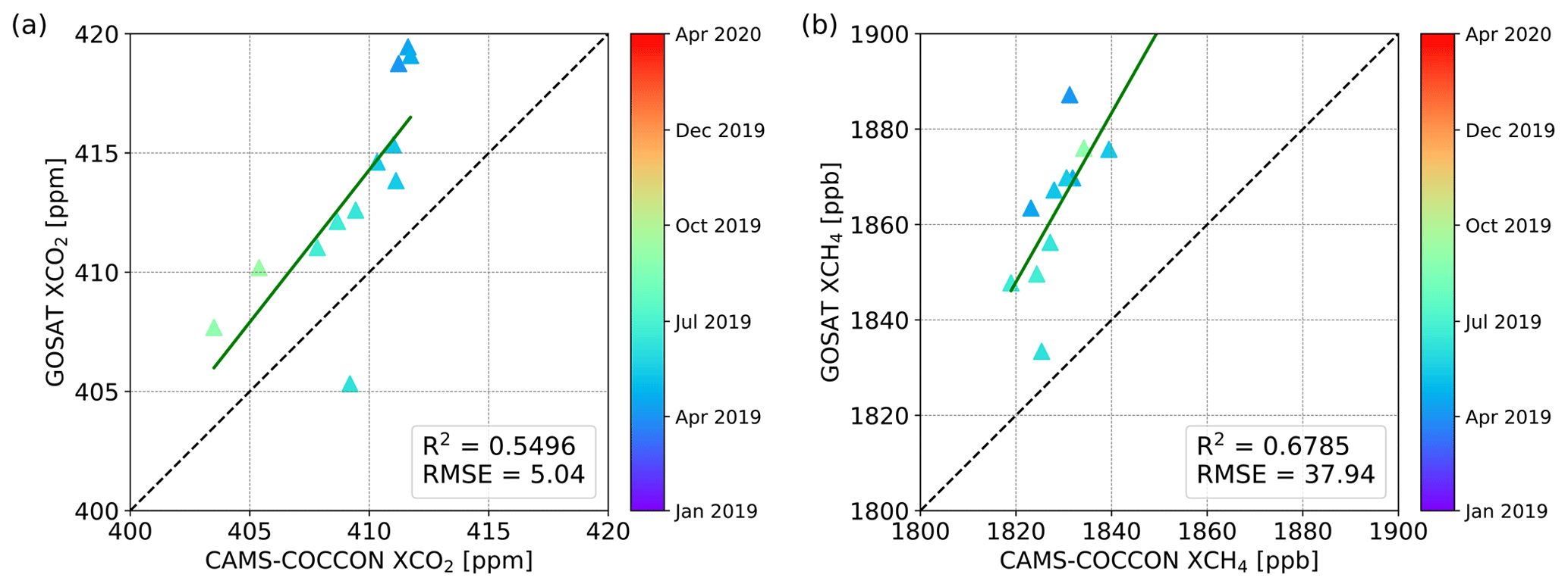
Figure 17Correlation plots of (a) GOSAT XCO2 and (b) GOSAT XCH4 with respect to CAMS-COCCON at Peterhof. All satellite data were adjusted for the CAMS a priori profile.
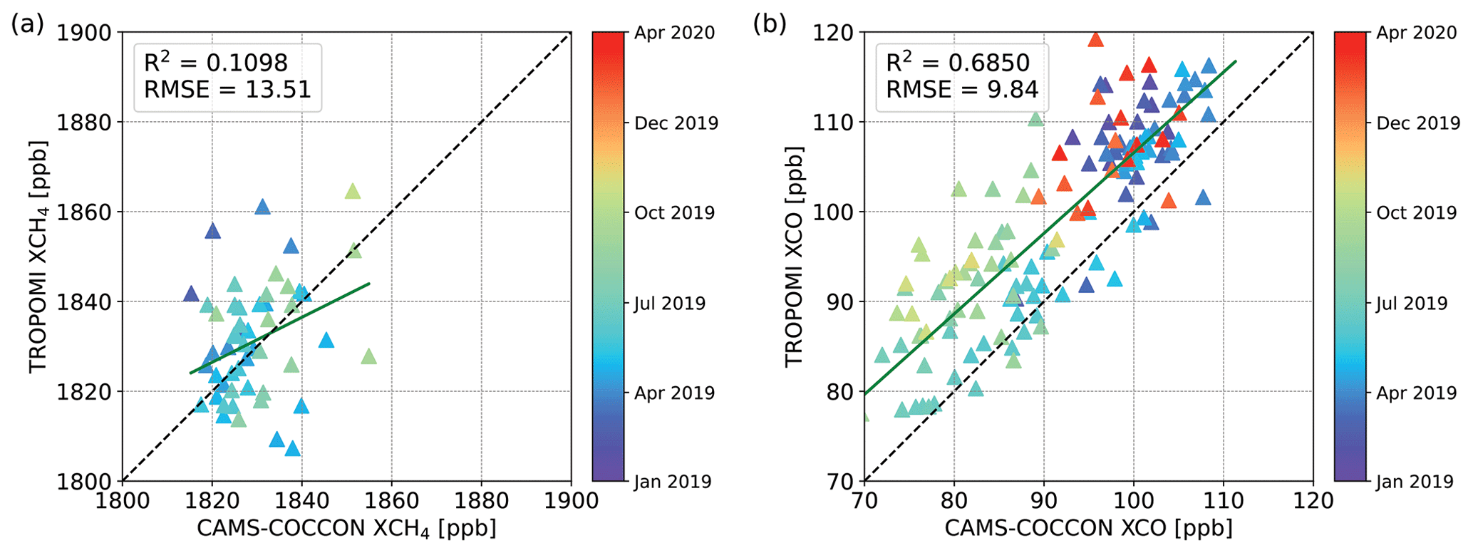
Figure 18Correlation plots of (a) TROPOMI XCH4 and (b) TROPOMI XCO with respect to CAMS-COCCON at Peterhof. All satellite data were adjusted for the CAMS a priori profile.
4.5.2 Yekaterinburg
The scaled data are much more important in Yekaterinburg, because in this city there are just a few coincident measurement days between the COCCON spectrometer and satellite results, mainly because of the season of the measurements taken in winter and spring. That makes a real challenge in finding the best number of sub-windows to better adjust COCCON to CAMS results, which is rather small (between 2 and 3). Nevertheless, as can be seen in Fig. A13 and Table A3, the CAMS-COCCON data agree better with the coincident COCCON observations, which indicates that the scaling improves the compatibility of CAMS data with COCCON, although the number of sampling points is extremely small.
The correlations between CAMS-COCCON and the OCO-2 and TROPOMI data are presented in Fig. 19. There are not too many coincident data points than those at Peterhof due to the lesser COCCON and satellite observations and mostly poor weather condition in winter. The COCCON measurement ended on 17 April 2020. Here we use a larger radius (100 km) to collect TROPOMI data for coincident COCCON observations.
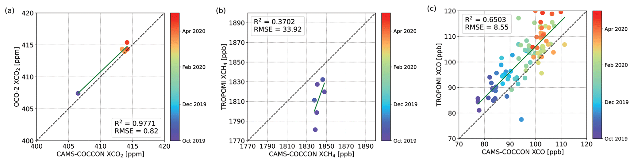
Figure 19Correlation plots of (a) XCO2 between OCO-2 and CAMS-COCCON, (b) XCH4 between TROPOMI and CAMS-COCCON, and (c) XCO between TROPOMI and CAMS-COCCON observations at Yekaterinburg. All satellite data were adjusted for the CAMS a priori profile.
The averaged biases between satellite products with respect to CAMS-COCCON are presented in Fig. 20. Table 4 summarizes selected biases and standard deviations of satellite products compared to COCCON and CAMS-COCCON data. Here, only when the coincident data between satellite observations and COCCON and CAMS-COCCON are both available (at least at one site) are they shown. For XCO2, the biases decrease slightly when OCO-2 is compared with COCCON and to CAMS-COCCON. The absolute bias between TROPOMI XCH4 and CAMS-COCCON increased mostly twice at both sites in comparison to the direct TROPOMI XCH4 to COCCON comparison. The increased low bias at Peterhof is mainly driven by the TROPOMI outliers in April (Fig. 8b). The increased low bias at Yekaterinburg is due to the fact that the CAMS-COCCON data are only available up to the end of 2019, and all TROPOMI data in autumn 2019 are biased low (Fig. 9b). For XCO, the bias increased slightly at Peterhof and decreased by nearly half at Yekaterinburg when using CAMS-COCCON as the reference instead of COCCON at both sites.
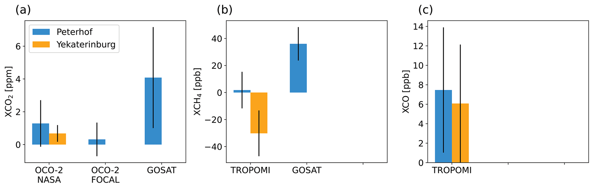
Figure 20Bar plots of the averaged bias derived from different products with respect to CAMS-COCCON for (a) XCO2, (b) XCH4 and (c) XCO at Peterhof and Yekaterinburg. The error bars represent the standard deviation of the bias.
Table 4Selected averaged bias and standard deviation between satellite products and COCCON and between satellite products and CAMS-COCCON at Peterhof and Yekaterinburg. The number of coincident results is shown in parentheses.
* No CAMS XCH4 in 2020.
4.5.3 Gradients between Peterhof and Yekaterinburg
For the comparison shown in this section, the COCCON-CAMS product by using CAMS-Xgas a priori data have been used. This choice removes the comparisons for XCH4 in 2020 for both cities, because no XCH4 from CAMS is available by now.
The gradients (ΔXgas) are the difference of each product between the two sites during the same time period. The gradients between Peterhof and Yekaterinburg (Peterhof–Yekaterinburg) are presented in Fig. 21. The measuring time of COCCON at Yekaterinburg is less than that at Peterhof. We therefore use monthly means at each site to compute the gradients. A collecting circle with a radius of 100 km is used for TROPOMI at both sites. The coincident measurement days at both sites start from October 2019 until April 2020.
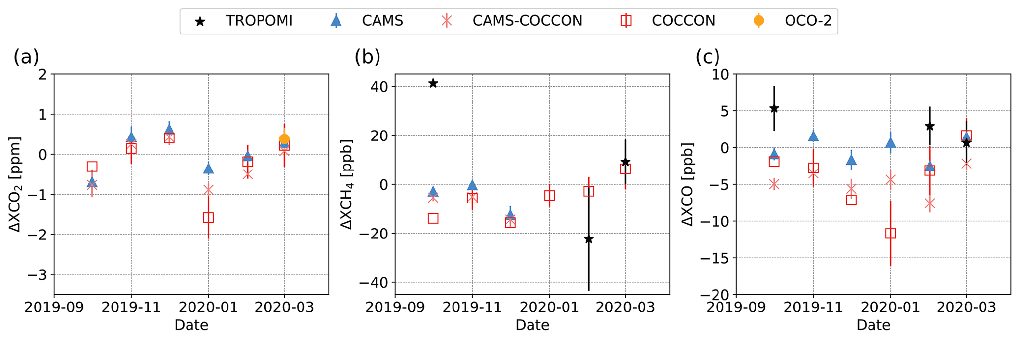
Figure 21Monthly mean of gradients for different gases (ΔXgas) between Peterhof and Yekaterinburg (Peterhof–Yekaterinburg) for different products. The error bars are calculated based on the standard deviation at two sites.
For XCO2, the gradients between COCCON at both sites are mostly negative and lower than those of CAMS and CAMS-COCCON datasets. Higher absolute gradients are observed in the early part of the year for COCCON. In November and December both CAMS and CAMS-COCCON ΔXCO2 show positive values, whereas COCCON has negative values. This discrepancy might be due to the limited number of COCCON observations during winter in Yekaterinburg (only 12 d of measurements from November to Mach were available). The gradients of different datasets generally fit well for XCH4, except that of TROPOMI in October due to the low number of observations in winter. COCCON ΔXCO shows highest absolute value in January, when the CAMS value is near to zero. The large variations in ΔXCO are in reasonable agreement with the COCCON gradients.
4.5.4 St Petersburg city emission transport event tracked by TROPOMI
The results of the EMME campaign are described in detail and analysed in Makarova et al. (2021) and Ionov et al. (2021); nevertheless, none of these studies performed any satellite comparison so far. Therefore, in this subsection we show how a satellite with a high temporal and spatial resolution can measure and track a large transport of pollutants in a megacity like St Petersburg. During the EMME campaign, we have been lucky to have the overpass of the TROPOMI satellite during one of the days with strong transport gradient as presented in Makarova et al. (2021). Such results are presented in Fig. 22, which illustrates the XCH4 and XCO observations on a sample day on 25 April 2019 when the wind flowed from northeast to east before noon. The coincident TROPOMI data are the mean value collected within a circle of 15 km radius. The downwind COCCON instrument FTS#84 measured significant enhancements of XCH4 and XCO around 09:00 UTC. The higher XCH4 measured by FTS#84 than that by FTS#80 is later observed by TROPOMI as well at 10:40 UTC, though the absolute values are lower in TROPOMI than the corresponding COCCON observations. When comparing the observations with COCCON and TROPOMI at the two locations where the spectrometers were set up on that day, the measured differences are about 10.6 ppb and 9.4 ppb for COCCON and TROPOMI, respectively (Fig. 22e – bottom panel). For XCO, TROPOMI observes higher values than COCCON. The difference between the two locations at 10:40 UTC is 9.5 ppb for COCCON and 12.5 ppb for TROPOMI. The increase in XCO at the FTS#80 location measured by COCCON can also be detected by TROPOMI, as it increased from 107.0 to 115.7 ppb.
When comparing the observations with COCCON and TROPOMI in each of two places where the spectrometers were setup on that day, at the TROPOMI overpassing time 10:40 UTC, the measured difference (delta) is 10.6 ppb and 9.5ppb for COCCON and TROPOMI respectively.
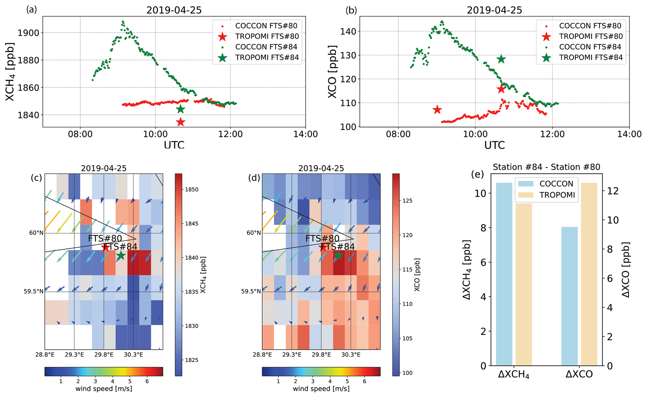
Figure 22Time series of COCCON and coincident TROPOMI observations for XCH4 (a) and XCO (b); spatial distribution of XCH4 (c) and XCO (d) on a latitude × longitude grid together with the ERA5 wind at 12:00 UTC; (e) bar plot for XCH4 and XCO gradients by COCCON and TROPOMI on 25 April 2019.
The present study analyses ground-based COCCON and space-based TROPOMI, OCO-2, OCO-2 FOCAL, GOSAT and MUSICA IASI observations (XCO2, XCH4, XCO, XH2O), supported by CAMS model data (XCO2, XCH4, XCO) in Peterhof and Yekaterinburg cities located at high latitudes. Such stationary observations were performed during 2019–2020, and a mobile city campaign was carried out in St Petersburg in 2019 within the framework of the VERIFY project.
All the data products in Peterhof show similar seasonal variability. However, for XCO2, the COCCON dataset is generally lower than the other available datasets, among which GOSAT has the highest standard deviation compared to the other datasets. TROPOMI observes slightly lower XCH4 but slightly higher XCO than the other products. The largest seasonal variability is seen in XH2O. Higher amounts of XH2O are observed in summer, mostly due to higher evaporation and precipitation, which is expected. The averaged GOSAT XH2O is higher than the other products due to its short measurement period, which is mostly in summer. There is a shorter measurement period in Yekaterinburg, covering mostly winter and spring, from October 2019 to April 2020. Similar seasonality and concentrations are observed to those in Peterhof at the same time period.
The satellite observations are sparser in the high-latitude regions than in mid- and low-latitude regions, while models provide continuous datasets. The ground-based COCCON observations have proven to be highly accurate by many previous studies. To combine the advantages of CAMS and COCCON datasets, we developed an upscaling method by adjusting CAMS data to the COCCON observations collected at Peterhof and Yekaterinburg to obtain a continuous data of virtual COCCON observations (as demonstrated using different subsets of COCCON measurements at Karlsruhe). This method is more important for Yekaterinburg, where we face three different problems: (1) fewer measurements in general (around 6 months compared to 15 months in Peterhof), (2) fewer measurement days per month (mostly in winter) and (3) shorter daily period of measurements. As expected, the CAMS-COCCON data show better correlations with COCCON observations than the original CAMS datasets. The CAMS-COCCON data are then compared with satellite products, showing good agreements as well and generally similar biases to those between satellite products and COCCON observations. This method was also used for the observations at Yekaterinburg where fewer COCCON measurements were taken. The gradients between the two study sites (ΔXgas) are similar between CAMS and CAMS-COCCON datasets. There are a few COCCON and satellite ΔXgas measurements fitting well to those of CAMS-COCCON. The results presented in this study indicate that our scaling method is working reliably.
In addition, the XCH4 and XCO observations recorded during one of the mobile city campaign days (25 April 2019) were analysed. In the city campaign, two COCCON instruments were set up in the upwind and downwind sites, and the wind flowed from northeast to east before noon on the sample day. The downwind COCCON instrument measured obvious enhancements in both XCH4 (10.6 ppb) and XCO (9.5 ppb), which is also observed by TROPOMI (9.4 ppb in XCH4 and 12.5 ppb XCO, respectively).
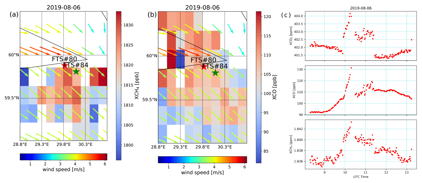
Figure A1Spatial distribution of XCH4 (a) and XCO (b) on a latitude × longitude grid together with the ERA5 wind at 12:00 UTC, and (c) daily time series of XCO2, XCO and XCH4 (top, middle and bottom panels, respectively) on 6 August 2019.
Table A1Overview of the satellite and model data products used in this study.
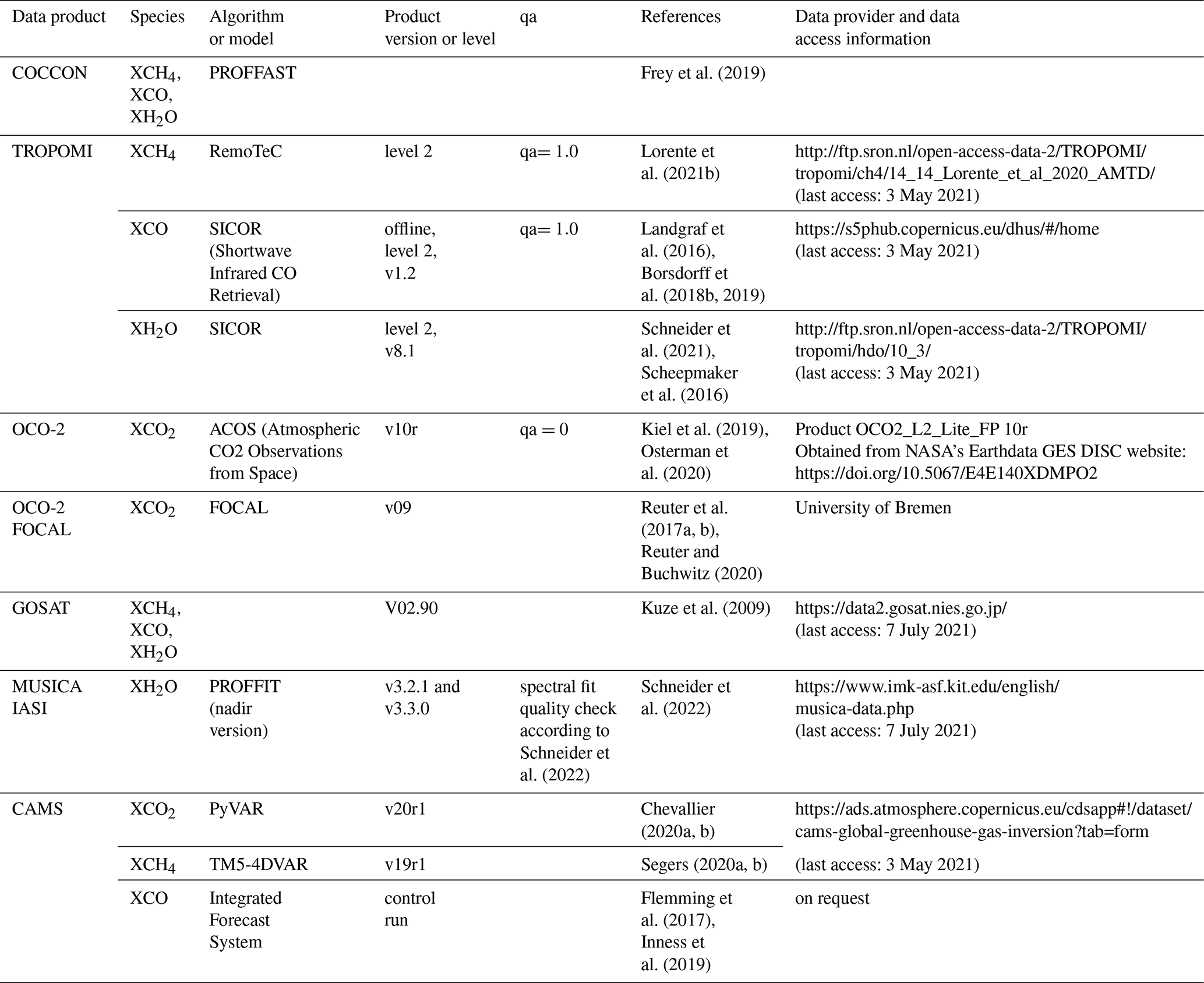

Figure A2(a) Spatial distribution of CO emissions (tonnes per ∘ yr−1) from “Sector-Specific Gridmaps”: combustion for manufacturing. Data source: EDGAR v5.0, 2015 (https://edgar.jrc.ec.europa.eu/dataset_ap50, last access: 4 August 2021); the map was generated with Python basemap toolkit by using ArcGIS from a world shaded relief model; (b) backward trajectories arriving in Peterhof on 6 August 2019, calculated by using the HYSPLIT model.
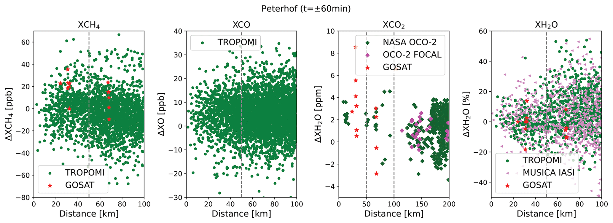
Figure A3Difference between a single satellite measurement with the averaged COCCON measurement (±1 h of satellite overpass) with respect to their distance.
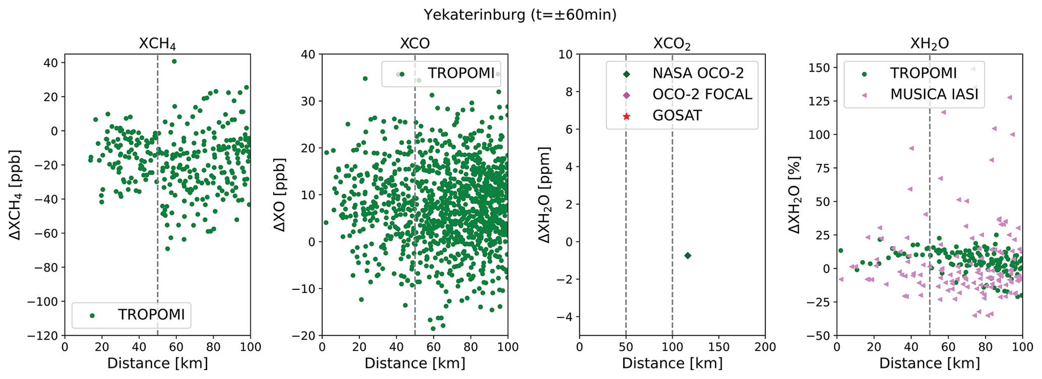
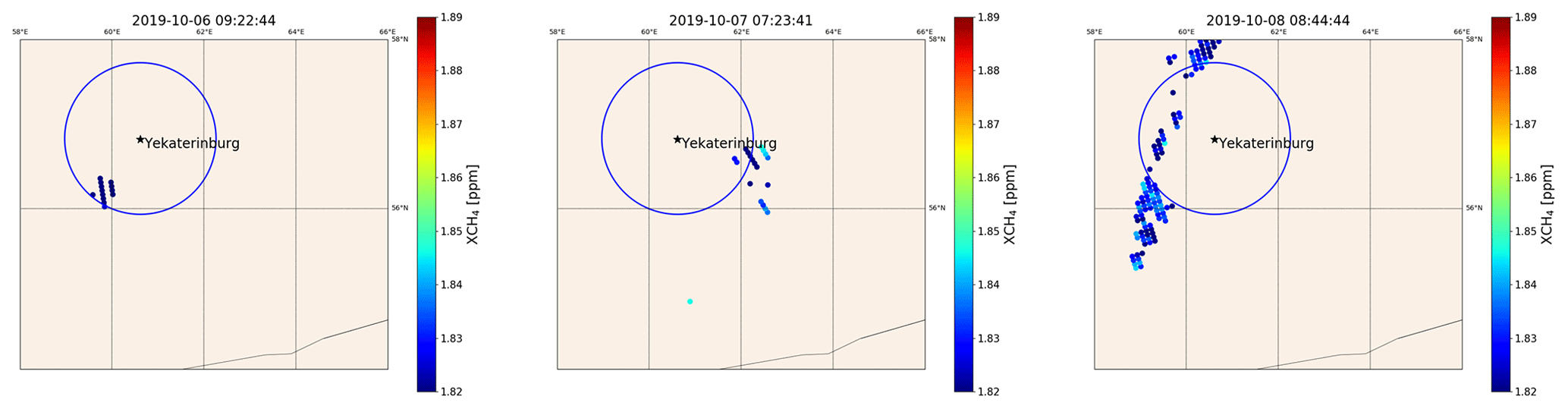
Figure A5Sample days for TROPOMI measurements (qa =1.0) in October 2019. The circle has a radius of 100 km, centred at Yekaterinburg. The colour represents the value of XCH4.
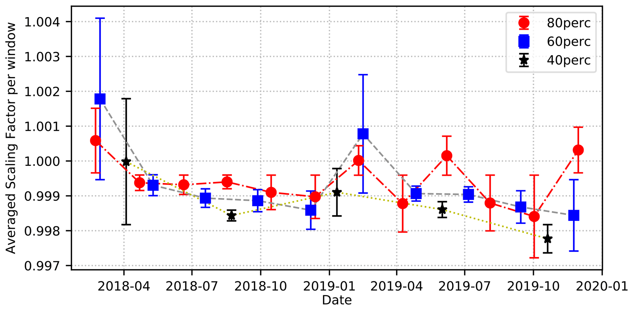
Figure A6Temporal variation of the averaged scaling factors in each sub-window for the number of windows selected for each subset of COCCON measurements at Karlsruhe (40 %, 60 % and 80 % of the total measurement days with FTS#37). The error bar represents the standard deviation calculated in each sub-window.
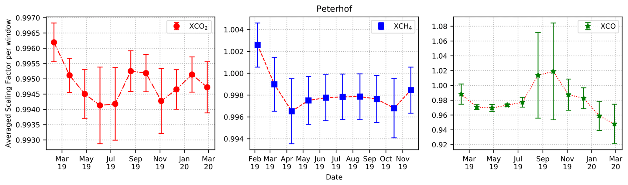
Figure A7Temporal variation of the averaged scaling factors per window for each studied gas: XCO2, XCH4 and XCO at Peterhof.
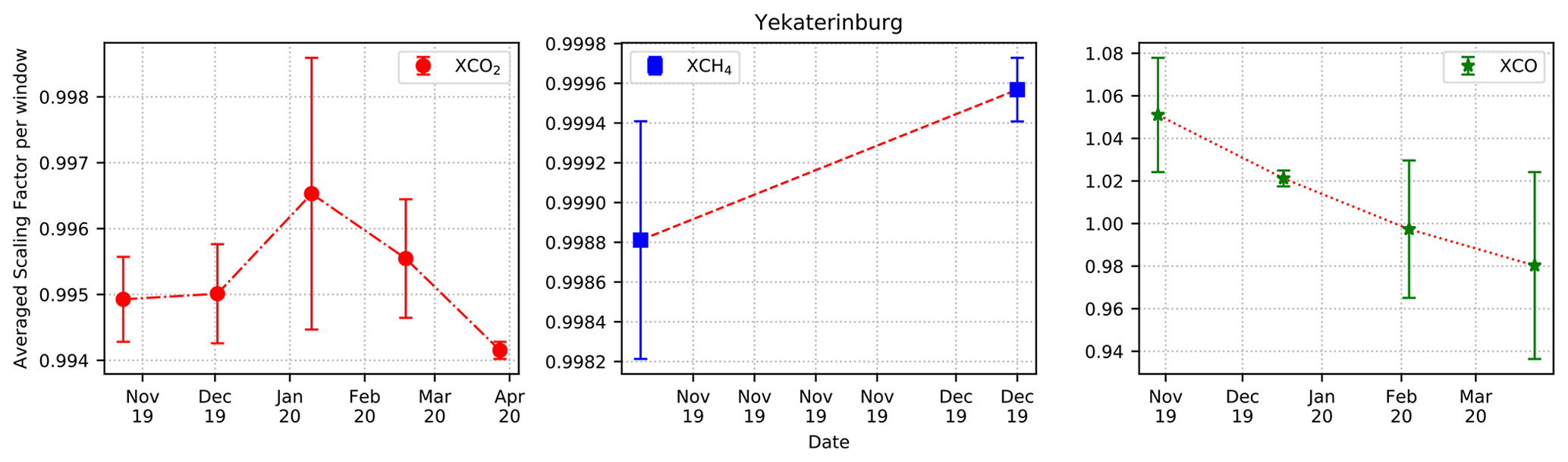
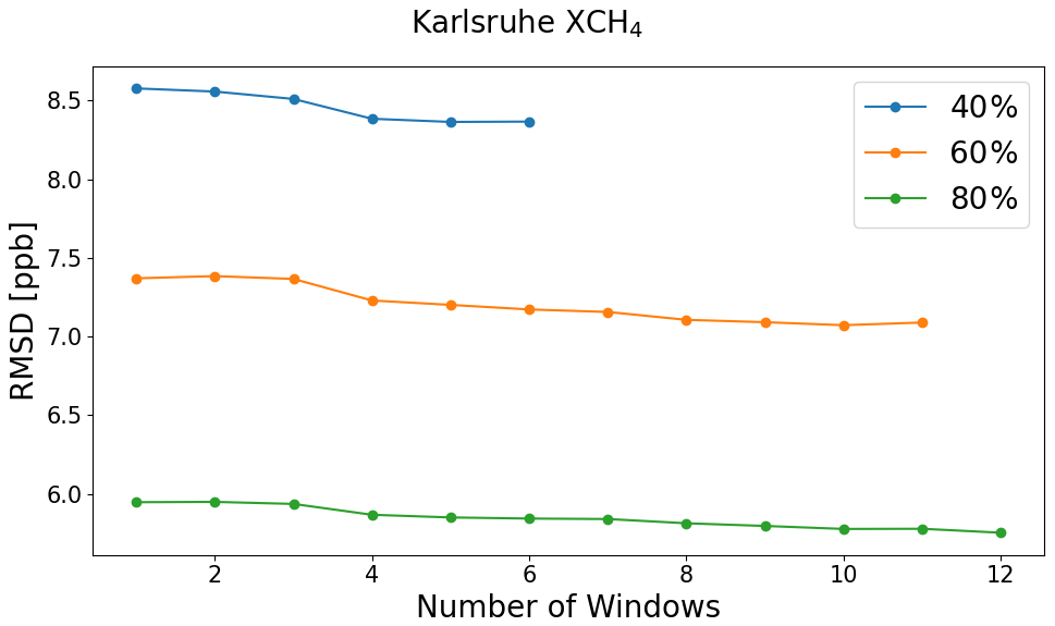
Figure A9Root-mean-square deviation between CAMS-COCCON and COCCON with respect to number of windows for XCH4 according to 40 %, 60 % and 80 % COCCON data points at Karlsruhe.
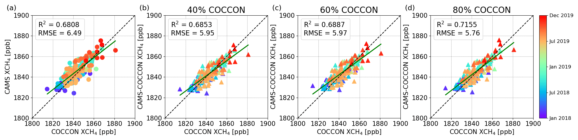
Figure A10Correlation plots of (a) CAMS and (b–d) CAMS-COCCON with respect to COCCON XCH4 at Karlsruhe. The CAMS-COCCON datasets are based on 40 %, 60 % and 80 % of COCCON measurement days.
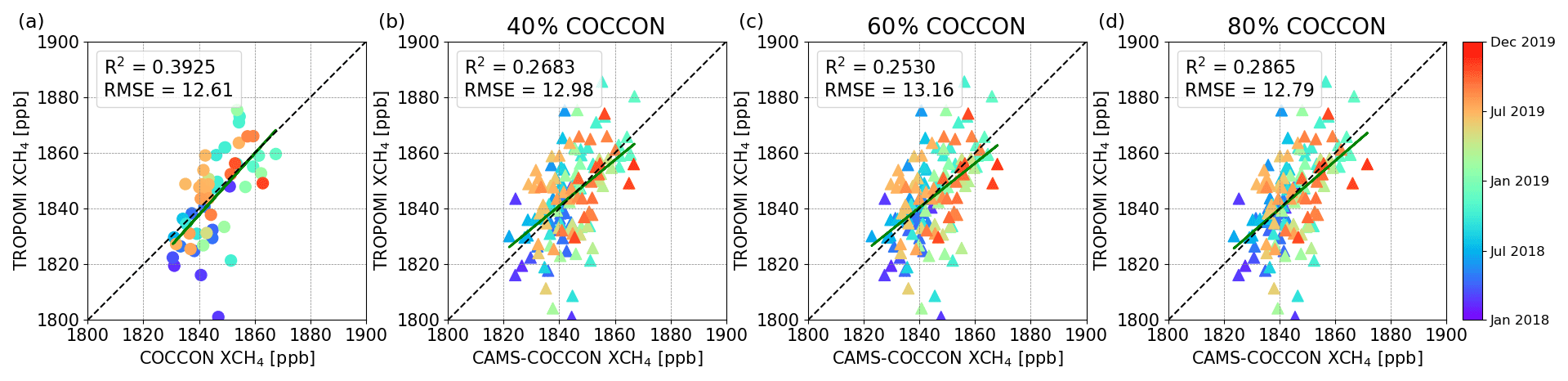
Figure A11Correlation plots of (a) COCCON and (b–d) CAMS-COCCON with respect to TROPOMI XCH4 at Karlsruhe. The CAMS-COCCON datasets are based on 40 %, 60 % and 80 % of COCCON measurement days.
Table A2Number of TROPOMI measurements within 50 km and within 100 km.
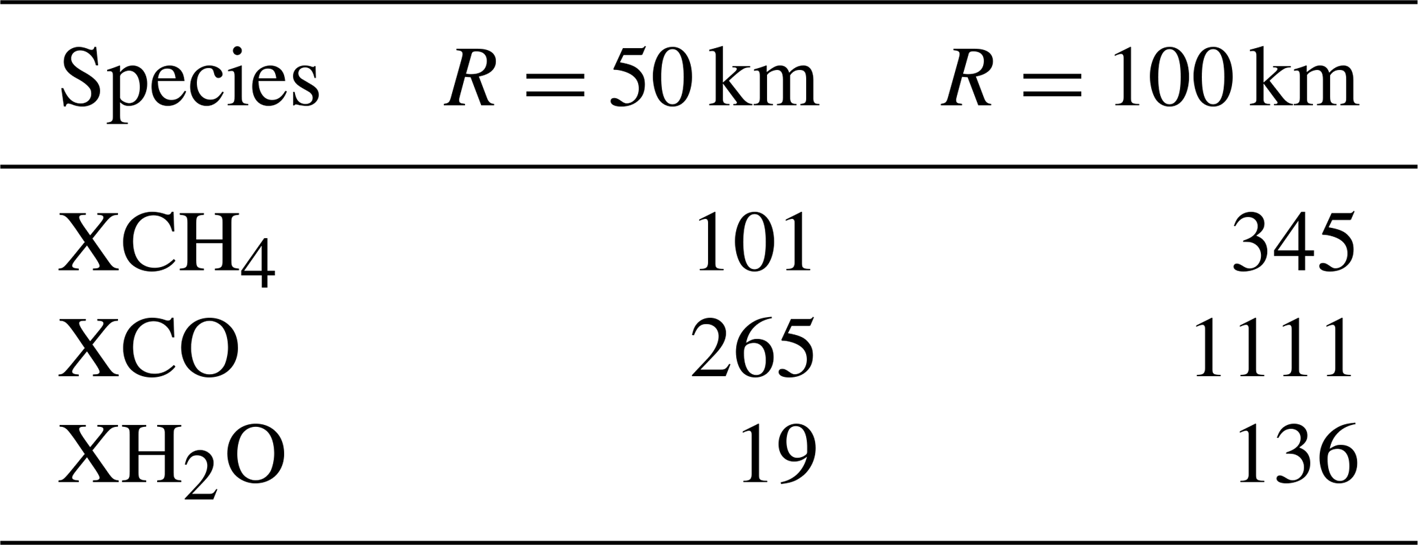
Table A3The variability (standard deviation) of the original CAMS products during the COCCON measurement period in each city and bias and standard deviation for the difference between CAMS and COCCON, as well as between scaled CAMS and COCCON.
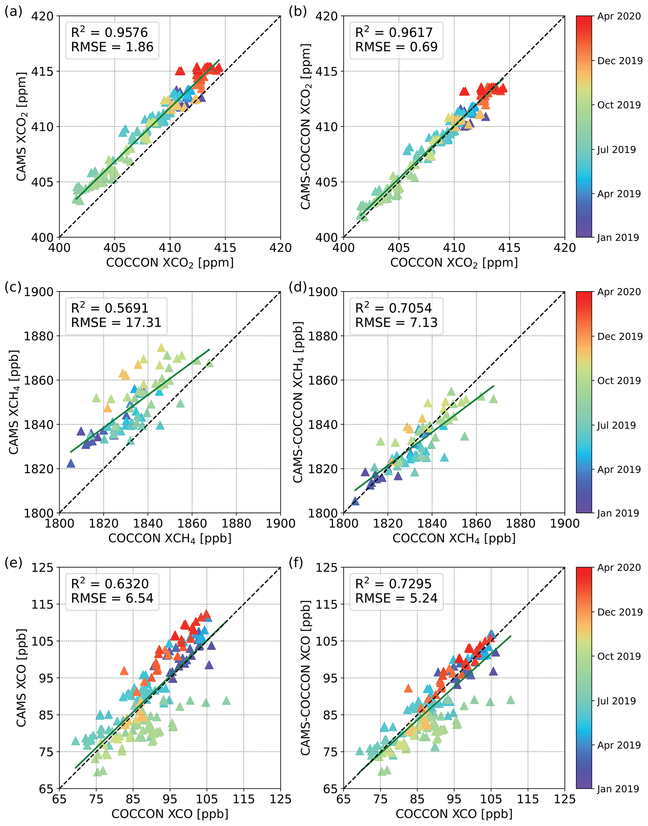
Figure A12Correlation plots of CAMS (a, c, e) and CAMS-COCCON (b, d, f) with respect to COCCON for XCO2 (a, b), XCH4 (c, d) and XCO (e, f) at Peterhof.
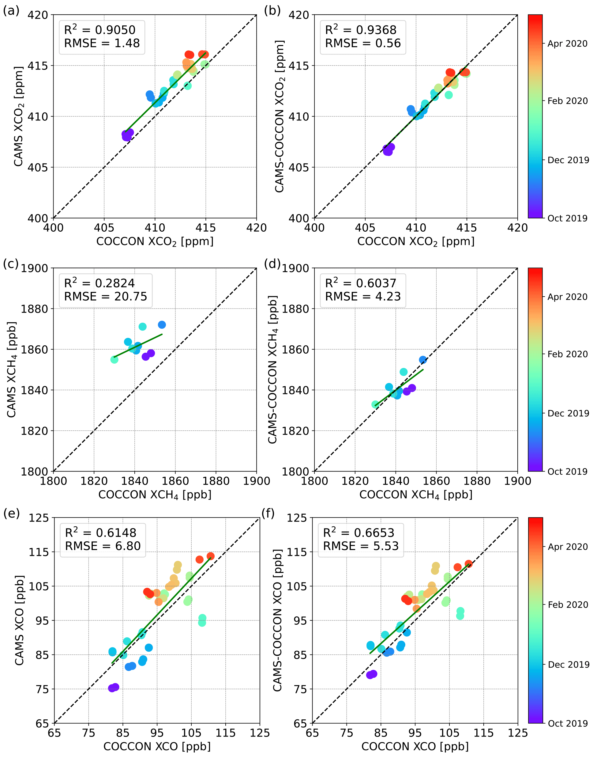
Figure A13Correlation plots of CAMS (a, c, e) and CAMS-COCCON (b, d, f) with respect to COCCON for XCO2 (a, b), XCH4 (c, d) and XCO (e, f) at Yekaterinburg.
The data are accessible by contacting the authors (carlos.alberti@kit.edu and qiansi.tu@kit.edu). The OCO-2 data product is publicly available through the NASA Goddard Earth Science Data and Information Services Center (GES DISC) for distribution and archiving (http://disc.sci.gsfc.nasa.gov/OCO-2; last access: 6 May 2021). The OCO-2 FOCAL XCO2 v09 product can be obtained from the OCO-2 FOCAL website (http://www.iup.uni-bremen.de/~mreuter/focal.php, last access: 3 August 2021). The SRON S5P-RemoTeC scientific TROPOMI CH4 dataset from this study is available for download at https://doi.org/10.5281/zenodo.4447228 (Lorente et al., 2021a). The S5-P H2O dataset from this study is available for download at http://ftp.sron.nl/open-access-data-2/TROPOMI/tropomi/hdo/10_3/ (last access: 6 May 2021; Schneider et al., 2021; https://doi.org/10.5194/amt-2021-141). The S5-P CH4 and CO datasets are publicly available from https://scihub.copernicus.eu/ (last access: 6 April 2022; Copernicus Open Access Hub, 2020). The access and use of any Copernicus Sentinel data available through the Copernicus Open Access Hub are governed by the legal notice on the use of Copernicus Sentinel Data and Service Information, which is given here: https://sentinels.copernicus.eu/documents/247904/690755/Sentinel_Data_Legal_Notice (last access: 6 May 2021; European Commission, 2020). The GOSAT TANSO-FTS SWIR L2 data are available from the GOSAT Data Archive Service (GDAS) at https://data2.gosat.nies.go.jp/ (last access: 6 April 2022; GDAS, 2022).
CA and QT developed the research question, performed the data analysis and wrote the article with support from FH. MS, BE, CD and FK provided the MUSICA data. MMF supported the instrument calibration at KIT before the campaign. MVM, SCF and SIO carried out stationary observations at the Peterhof site (SPbU) and processed raw EM27/SUN data. MB and MR revised and contributed to the improvement of the article. MVM, KG, VZ, DVI, FK, MMF, MS, MR, MB, TB and TW proofread the manuscript.
The contact author has declared that neither they nor their co-authors have any competing interests.
The CAMS results were generated using Copernicus Atmosphere Monitoring Service (2017–2020) information. Neither the European Commission nor ECMWF is responsible for any use that may be made of the Copernicus information or
data it contains.
Publisher’s note: Copernicus Publications remains neutral with regard to jurisdictional claims in published maps and institutional affiliations.
We thank Michela Giusti in the Data Support Team at ECMWF for retrieving and providing comments about the CAMS data. We are grateful to Yuri Timofeyev for his insightful comments on the manuscript.
This research has been supported by the European Commission, Horizon 2020 Framework Programme (VERIFY (grant no. 776810)),
the University of Bremen received co-funding from ESA (GHG-CCIC+ project) for the generation and data analysis of the FOCAL product. Activity by Konstantin
Gribanov was partially supported in the framework of the state assignment project FEUZ-2020-0057, and the activity of Vyacheslav Zakharov was supported in the framework of the Russian Science Foundation (grant no. 18-11-00024-Π).
The article processing charges for this open-access publication were covered by the Karlsruhe Institute of Technology (KIT).
This paper was edited by Kimberly Strong and reviewed by three anonymous referees.
Alberti, C., Hase, F., Frey, M., Dubravica, D., Blumenstock, T., Dehn, A., Surawicz, G., Harig, R., Orphal, J., and the EM27/SUN-partners team: Improved calibration procedures for the EM27/SUN spectrometers of the COllaborative Carbon Column Observing Network (COCCON), Atmos. Meas. Tech. Discuss. [preprint], https://doi.org/10.5194/amt-2021-395, in review, 2021.
Bergamaschi, P., Krol, M., Meirink, J. F., Dentener, F., Segers, A., van Aardenne, J., Monni, S., Vermeulen, A. T., Schmidt, M., Ramonet, M., Yver, C., Meinhardt, F., Nisbet, E. G., Fisher, R. E., O'Doherty, S., and Dlugokencky, E. J.: Inverse modeling of European CH4 emissions 2001–2006, J. Geophys. Res., 115, D22309, https://doi.org/10.1029/2010JD014180, 2010.
Bergamaschi, P., Houweling, S., Segers, A., Krol, M., Frankenberg, C., Scheepmaker, R. A., Dlugokencky, E., Wofsy, S. C., Kort, E. A., Sweeney, C., Schuck, T., Brenninkmeijer, C., Chen, H., Beck, V., and Gerbig, C.: Atmospheric CH4 in the first decade of the 21st century: Inverse modeling analysis using SCIAMACHY satellite retrievals and NOAA surface measurements, J. Geophys. Res.-Atmos., 118, 7350–7369, https://doi.org/10.1002/jgrd.50480, 2013.
Borger, C., Schneider, M., Ertl, B., Hase, F., García, O. E., Sommer, M., Höpfner, M., Tjemkes, S. A., and Calbet, X.: Evaluation of MUSICA IASI tropospheric water vapour profiles using theoretical error assessments and comparisons to GRUAN Vaisala RS92 measurements, Atmos. Meas. Tech., 11, 4981–5006, https://doi.org/10.5194/amt-11-4981-2018, 2018.
Borsdorff, T., Aan de Brugh, J., Hu, H., Aben, I., Hasekamp, O., and Landgraf, J.: Measuring Carbon Monoxide With TROPOMI: First Results and a Comparison With ECMWF-IFS Analysis Data, Geophys. Res. Lett., 45, 2826–2832, https://doi.org/10.1002/2018GL077045, 2018a.
Borsdorff, T., aan de Brugh, J., Hu, H., Hasekamp, O., Sussmann, R., Rettinger, M., Hase, F., Gross, J., Schneider, M., Garcia, O., Stremme, W., Grutter, M., Feist, D. G., Arnold, S. G., De Mazière, M., Kumar Sha, M., Pollard, D. F., Kiel, M., Roehl, C., Wennberg, P. O., Toon, G. C., and Landgraf, J.: Mapping carbon monoxide pollution from space down to city scales with daily global coverage, Atmos. Meas. Tech., 11, 5507–5518, https://doi.org/10.5194/amt-11-5507-2018, 2018b.
Borsdorff, T., aan de Brugh, J., Schneider, A., Lorente, A., Birk, M., Wagner, G., Kivi, R., Hase, F., Feist, D. G., Sussmann, R., Rettinger, M., Wunch, D., Warneke, T., and Landgraf, J.: Improving the TROPOMI CO data product: update of the spectroscopic database and destriping of single orbits, Atmos. Meas. Tech., 12, 5443–5455, https://doi.org/10.5194/amt-12-5443-2019, 2019.
Butz, A., Dinger, A. S., Bobrowski, N., Kostinek, J., Fieber, L., Fischerkeller, C., Giuffrida, G. B., Hase, F., Klappenbach, F., Kuhn, J., Lübcke, P., Tirpitz, L., and Tu, Q.: Remote sensing of volcanic CO2, HF, HCl, SO2, and BrO in the downwind plume of Mt. Etna, Atmos. Meas. Tech., 10, 1–14, https://doi.org/10.5194/amt-10-1-2017, 2017.
Chen, J., Viatte, C., Hedelius, J. K., Jones, T., Franklin, J. E., Parker, H., Gottlieb, E. W., Wennberg, P. O., Dubey, M. K., and Wofsy, S. C.: Differential column measurements using compact solar-tracking spectrometers, Atmos. Chem. Phys., 16, 8479–8498, https://doi.org/10.5194/acp-16-8479-2016, 2016.
Chevallier, F.: Description of the CO2 inversion production chain, CAMS deliverable CAMS73_2018SC2_D73.5.2.1-2020_202004_CO2 inversion production chain_v1, https://atmosphere.copernicus.eu/ (last access: 6 April 2022), 2020a.
Chevallier, F.: Validation report for the CO2 fluxes estimated by atmospheric inversion, v20r1 Version 1.0, CAMS deliverable CAMS73_2018SC2_D73.1.4.1-2019_v4_202011_Validation inversion CO2, https://atmosphere.copernicus.eu/ (last access: 6 April 2022), 2020b
Clerbaux, C., Boynard, A., Clarisse, L., George, M., Hadji-Lazaro, J., Herbin, H., Hurtmans, D., Pommier, M., Razavi, A., Turquety, S., Wespes, C., and Coheur, P.-F.: Monitoring of atmospheric composition using the thermal infrared IASI/MetOp sounder, Atmos. Chem. Phys., 9, 6041–6054, https://doi.org/10.5194/acp-9-6041-2009, 2009.
Connor, B. J., Boesch, H., Toon, G., Sen, B., Miller, C., and Crisp, D.: Orbiting Carbon Observatory: Inverse method and prospective error analysis, J. Geophys. Res., 113, D05305, https://doi.org/10.1029/2006JD008336, 2008.
Copernicus Open Access Hub: https://scihub.copernicus.eu/, last access: 6 April 2022.
Crisp, D.: Measuring atmospheric carbon dioxide from space with the Orbiting Carbon Observatory-2 (OCO-2), Proc. SPIE 9607, Earth Observing Systems XX, 960702 (8 September 2015), https://doi.org/10.1117/12.2187291, 2015.
Cullis, C. F. and Willatt, B. M.: Oxidation of methane over supported precious metal catalysts, J. Catal., 83, 267–285, https://doi.org/10.1016/0021-9517(83)90054-4, 1983.
Dietrich, F., Chen, J., Voggenreiter, B., Aigner, P., Nachtigall, N., and Reger, B.: MUCCnet: Munich Urban Carbon Column network, Atmos. Meas. Tech., 14, 1111–1126, https://doi.org/10.5194/amt-14-1111-2021, 2021.
Eldering, A., Wennberg, P. O., Crisp, D., Schimel, D. S., Gunson, M. R., Chatterjee, A., Liu, J., Schwandner, F. M., Sun, Y., O'Dell, C. W., Frankenberg, C., Taylor, T., Fisher, B., Osterman, G. B., Wunch, D., Hakkarainen, J., Tamminen, J., and Weir, B.: The Orbiting Carbon Observatory-2 early science investigations of regional carbon dioxide fluxes, Science, 358, eaam5745, https://doi.org/10.1126/science.aam5745, 2017.
Flemming, J., Benedetti, A., Inness, A., Engelen, R. J., Jones, L., Huijnen, V., Remy, S., Parrington, M., Suttie, M., Bozzo, A., Peuch, V.-H., Akritidis, D., and Katragkou, E.: The CAMS interim Reanalysis of Carbon Monoxide, Ozone and Aerosol for 2003–2015, Atmos. Chem. Phys., 17, 1945–1983, https://doi.org/10.5194/acp-17-1945-2017, 2017.
Foka, S. C., Makarova, M. V., Ionov, D. V., Poberovskiy, A. V., Paramonova, N. N., and Ivakhov, V. M.: Evaluation of methane emission intensities for agglomeration territory of Saint-Petersburg, in: Proc. SPIE, 11560, https://doi.org/10.1117/12.2573232, 2020.
Frey, M., Hase, F., Blumenstock, T., Groß, J., Kiel, M., Mengistu Tsidu, G., Schäfer, K., Sha, M. K., and Orphal, J.: Calibration and instrumental line shape characterization of a set of portable FTIR spectrometers for detecting greenhouse gas emissions, Atmos. Meas. Tech., 8, 3047–3057, https://doi.org/10.5194/amt-8-3047-2015, 2015.
Frey, M., Sha, M. K., Hase, F., Kiel, M., Blumenstock, T., Harig, R., Surawicz, G., Deutscher, N. M., Shiomi, K., Franklin, J. E., Bösch, H., Chen, J., Grutter, M., Ohyama, H., Sun, Y., Butz, A., Mengistu Tsidu, G., Ene, D., Wunch, D., Cao, Z., Garcia, O., Ramonet, M., Vogel, F., and Orphal, J.: Building the COllaborative Carbon Column Observing Network (COCCON): long-term stability and ensemble performance of the EM27/SUN Fourier transform spectrometer, Atmos. Meas. Tech., 12, 1513–1530, https://doi.org/10.5194/amt-12-1513-2019, 2019.
Frey, M. M., Hase, F., Blumenstock, T., Dubravica, D., Groß, J., Göttsche, F., Handjaba, M., Amadhila, P., Mushi, R., Morino, I., Shiomi, K., Sha, M. K., de Mazière, M., and Pollard, D. F.: Long-term column-averaged greenhouse gas observations using a COCCON spectrometer at the high-surface-albedo site in Gobabeb, Namibia, Atmos. Meas. Tech., 14, 5887–5911, https://doi.org/10.5194/amt-14-5887-2021, 2021.
Gavrilov, N. M., Makarova, M. V., Poberovskii, A. V., and Timofeyev, Yu. M.: Comparisons of CH4 ground-based FTIR measurements near Saint Petersburg with GOSAT observations, Atmos. Meas. Tech., 7, 1003–1010, https://doi.org/10.5194/amt-7-1003-2014, 2014.
Gisi, M., Hase, F., Dohe, S., Blumenstock, T., Simon, A., and Keens, A.: XCO2-measurements with a tabletop FTS using solar absorption spectroscopy, Atmos. Meas. Tech., 5, 2969–2980, https://doi.org/10.5194/amt-5-2969-2012, 2012.
GOSAT Data Archive Service (GDAS): https://data2.gosat.nies.go.jp/index_en.html, last access: 6 April 2022.
Harris, P. G., Chow, A. S. Y., and Symons, J.: Greenhouse gas emissions from cities and regions: International implications revealed by Hong Kong, Energ. Policy, 44, 416–424, https://doi.org/10.1016/j.enpol.2012.02.012, 2012.
Hase, F., Frey, M., Blumenstock, T., Groß, J., Kiel, M., Kohlhepp, R., Mengistu Tsidu, G., Schäfer, K., Sha, M. K., and Orphal, J.: Application of portable FTIR spectrometers for detecting greenhouse gas emissions of the major city Berlin, Atmos. Meas. Tech., 8, 3059–3068, https://doi.org/10.5194/amt-8-3059-2015, 2015.
Hase, F., Frey, M., Kiel, M., Blumenstock, T., Harig, R., Keens, A., and Orphal, J.: Addition of a channel for XCO observations to a portable FTIR spectrometer for greenhouse gas measurements, Atmos. Meas. Tech., 9, 2303–2313, https://doi.org/10.5194/amt-9-2303-2016, 2016.
Hedelius, J. K., Viatte, C., Wunch, D., Roehl, C. M., Toon, G. C., Chen, J., Jones, T., Wofsy, S. C., Franklin, J. E., Parker, H., Dubey, M. K., and Wennberg, P. O.: Assessment of errors and biases in retrievals of , , XCO, and from a 0.5 cm−1 resolution solar-viewing spectrometer, Atmos. Meas. Tech., 9, 3527–3546, https://doi.org/10.5194/amt-9-3527-2016, 2016.
Inness, A., Ades, M., Agustí-Panareda, A., Barré, J., Benedictow, A., Blechschmidt, A.-M., Dominguez, J. J., Engelen, R., Eskes, H., Flemming, J., Huijnen, V., Jones, L., Kipling, Z., Massart, S., Parrington, M., Peuch, V.-H., Razinger, M., Remy, S., Schulz, M., and Suttie, M.: The CAMS reanalysis of atmospheric composition, Atmos. Chem. Phys., 19, 3515–3556, https://doi.org/10.5194/acp-19-3515-2019, 2019.
Ionov, D. V., Makarova, M. V., Hase, F., Foka, S. C., Kostsov, V. S., Alberti, C., Blumenstock, T., Warneke, T., and Virolainen, Y. A.: The CO2 integral emission by the megacity of St Petersburg as quantified from ground-based FTIR measurements combined with dispersion modelling, Atmos. Chem. Phys., 21, 10939–10963, https://doi.org/10.5194/acp-21-10939-2021, 2021.
IPCC: Global Warming of 1.5 ∘C. An IPCC Special Report on the impacts of global warming of 1.5 ∘C above pre-industrial levels and related global greenhouse gas emission pathways, in the context of strengthening the global response to the threat of climate change, sustainable development, and efforts to eradicate poverty, edited by: Masson-Delmotte, V., Zhai, P., Pörtner, H.-O., Roberts, D., Skea, J., Shukla, P. R., Pirani, A., Moufouma-Okia, W., Péan, C., Pidcock, R., Connors, S., Matthews, J. B. R., Chen, Y., Zhou, X., Gomis, M. I., Lonnoy, E., Maycock, T., Tignor, M., and Waterfield, T., 2019 Intergovernmental Panel on Climate Change, in press, 2018.
IPCC: Summary for Policymakers, in: Climate Change 2021: The Physical Science Basis. Contribution of Working Group I to the Sixth Assessment Report of the Intergovernmental Panel on Climate Change, edited by: Masson-Delmotte, V., Zhai, P., Pirani, A., Connors, S. L., Péan, C., Berger, S., Caud, N., Chen, Y., Goldfarb, L., Gomis, M. I., Huang, M., Leitzell, K., Lonnoy, E., Matthews, J. B. R., Maycock, T. K., Waterfield, T., Yelekçi, O., Yu, R., and Zhou, B., Cambridge University Press, in press, 2021.
Jacobs, N., Simpson, W. R., Wunch, D., O'Dell, C. W., Osterman, G. B., Hase, F., Blumenstock, T., Tu, Q., Frey, M., Dubey, M. K., Parker, H. A., Kivi, R., and Heikkinen, P.: Quality controls, bias, and seasonality of CO2 columns in the boreal forest with Orbiting Carbon Observatory-2, Total Carbon Column Observing Network, and EM27/SUN measurements, Atmos. Meas. Tech., 13, 5033–5063, https://doi.org/10.5194/amt-13-5033-2020, 2020.
Jones, T. S., Franklin, J. E., Chen, J., Dietrich, F., Hajny, K. D., Paetzold, J. C., Wenzel, A., Gately, C., Gottlieb, E., Parker, H., Dubey, M., Hase, F., Shepson, P. B., Mielke, L. H., and Wofsy, S. C.: Assessing urban methane emissions using column-observing portable Fourier transform infrared (FTIR) spectrometers and a novel Bayesian inversion framework, Atmos. Chem. Phys., 21, 13131–13147, https://doi.org/10.5194/acp-21-13131-2021, 2021.
Kasischke, E. S. and Bruhwiler, L. P.: Emissions of carbon dioxide, carbon monoxide, and methane from boreal forest fires in 1998, J. Geophys. Res., 107, 8146, https://doi.org/10.1029/2001JD000461, 2002.
Keppel-Aleks, G., Wennberg, P. O., and Schneider, T.: Sources of variations in total column carbon dioxide, Atmos. Chem. Phys., 11, 3581–3593, https://doi.org/10.5194/acp-11-3581-2011, 2011.
Kiel, M., O'Dell, C. W., Fisher, B., Eldering, A., Nassar, R., MacDonald, C. G., and Wennberg, P. O.: How bias correction goes wrong: measurement of affected by erroneous surface pressure estimates, Atmos. Meas. Tech., 12, 2241–2259, https://doi.org/10.5194/amt-12-2241-2019, 2019.
Klappenbach, F., Bertleff, M., Kostinek, J., Hase, F., Blumenstock, T., Agusti-Panareda, A., Razinger, M., and Butz, A.: Accurate mobile remote sensing of XCO2 and XCH4 latitudinal transects from aboard a research vessel, Atmos. Meas. Tech., 8, 5023–5038, https://doi.org/10.5194/amt-8-5023-2015, 2015.
Kuze, A., Suto, H., Nakajima, M., and Hamazaki, T.: Thermal and near infrared sensor for carbon observation Fourier-transform spectrometer on the Greenhouse Gases Observing Satellite for greenhouse gases monitoring, Appl. Optics, 48, 6716–6733, https://doi.org/10.1364/AO.48.006716, 2009.
Landgraf, J., aan de Brugh, J., Scheepmaker, R., Borsdorff, T., Hu, H., Houweling, S., Butz, A., Aben, I., and Hasekamp, O.: Carbon monoxide total column retrievals from TROPOMI shortwave infrared measurements, Atmos. Meas. Tech., 9, 4955–4975, https://doi.org/10.5194/amt-9-4955-2016, 2016.
Langerock, B., De Mazière, M., Hendrick, F., Vigouroux, C., Desmet, F., Dils, B., and Niemeijer, S.: Description of algorithms for co-locating and comparing gridded model data with remote-sensing observations, Geosci. Model Dev., 8, 911–921, https://doi.org/10.5194/gmd-8-911-2015, 2015.
Liu, Y., Wang, J., Yao, L., Chen, X., Cai, Z., Yang, D., Yin, Z., Gu, S., Tian, L., Lu, N., and Lyu, D.: The TanSat mission: preliminary global observations, Sci. Bull., 63, 1200–1207, https://doi.org/10.1016/j.scib.2018.08.004, 2018.
Lorente, A., Borsdorff, T., aan de Brugh, J., Landgraf, J., and Hasekamp, O.: SRON S5P - RemoTeC scientific TROPOMI XCH4 dataset, Zenodo [data set], https://doi.org/10.5281/zenodo.4447228, 2021a.
Lorente, A., Borsdorff, T., Butz, A., Hasekamp, O., aan de Brugh, J., Schneider, A., Wu, L., Hase, F., Kivi, R., Wunch, D., Pollard, D. F., Shiomi, K., Deutscher, N. M., Velazco, V. A., Roehl, C. M., Wennberg, P. O., Warneke, T., and Landgraf, J.: Methane retrieved from TROPOMI: improvement of the data product and validation of the first 2 years of measurements, Atmos. Meas. Tech., 14, 665–684, https://doi.org/10.5194/amt-14-665-2021, 2021b.
Makarova, M. V., Kirner, O., Timofeev, Yu. M., Poberovskii, A. V., Imkhasin, Kh. Kh., Osipov, S. I., and Makarov, B. K.: Analysis of methane total column variations in the atmosphere near St. Petersburg using ground-based measurements and simulations. Izv. Atmos. Ocean. Phys., 51, 177–185, https://doi.org/10.1134/S0001433815010089, 2015a.
Makarova, M. V., Kirner, O., Timofeev, Yu. M., Poberovskii, A. V., Imkhasin, Kh. Kh., Osipov, S. I., and Makarov, B. K.: Annual cycle and long-term trend of the methane total column in the atmosphere over the St. Petersburg region, Izv. Atmos. Ocean. Phys., 51, 431–438, https://doi.org/10.1134/S0001433815040088, 2015b.
Makarova, M. V., Alberti, C., Ionov, D. V., Hase, F., Foka, S. C., Blumenstock, T., Warneke, T., Virolainen, Y. A., Kostsov, V. S., Frey, M., Poberovskii, A. V., Timofeyev, Y. M., Paramonova, N. N., Volkova, K. A., Zaitsev, N. A., Biryukov, E. Y., Osipov, S. I., Makarov, B. K., Polyakov, A. V., Ivakhov, V. M., Imhasin, H. Kh., and Mikhailov, E. F.: Emission Monitoring Mobile Experiment (EMME): an overview and first results of the St. Petersburg megacity campaign 2019, Atmos. Meas. Tech., 14, 1047–1073, https://doi.org/10.5194/amt-14-1047-2021, 2021.
Meetham, A. R., Bottom, D. W., and Cayton, S.: Atmospheric Pollution: Its History, Origins, and Prevention, Elsevier, ISBN 9781483135847, 2016.
Meirink, J. F., Bergamaschi, P., and Krol, M. C.: Four-dimensional variational data assimilation for inverse modelling of atmospheric methane emissions: method and comparison with synthesis inversion, Atmos. Chem. Phys., 8, 6341–6353, https://doi.org/10.5194/acp-8-6341-2008, 2008.
Miller, S. M., Wofsy, S. C., Michalak, A. M., Kort, E. A., Andrews, A. E., Biraud, S. C., Dlugokencky, E. J., Eluszkiewicz, J., Fischer, M. L., Janssens-Maenhout, G., Miller, B. R., Miller, J. B., Montzka, S. A., Nehrkorn, T., and Sweeney, C.: Anthropogenic emissions of methane in the United States, P. Natl. Acad. Sci. USA, 110, 20018–20022, https://doi.org/10.1073/pnas.1314392110, 2013.
Nikitenko, A. A., Timofeev, Y. M., Berezin, I. A., Poberovskii, A. V, Virolainen, Y. A., and Polyakov, A. V: The Analysis of OCO-2 Satellite Measurements of CO2 in the Vicinity of Russian Cities, Atmos. Ocean. Opt., 33, 650–655, https://doi.org/10.1134/S1024856020060111, 2020.
Osterman, G., O'Dell, C., Eldering A., Fisher, B., Crisp, D., Cheng, C., Frankenberg, C., Lambert, A., Gunson, M., Mandrake, L., and Wunch, D.: Orbiting Carbon Observatory-2 and 3 (OCO-2 & OCO-3), Data Product User's Guide, Operational Level 2 Data Versions 10 and Lite File Version 10 and VEarly, Technical Report National Aeronautics and Space Administration, Jet Propulsion Laboratory, California Institute of Technology, Pasadena, USA, https://docserver.gesdisc.eosdis.nasa.gov/public/project/OCO/OCO2_OCO3_B10_DUG.pdf (last access: 3 May 2021), 2020.
Patra, P. K., Crisp, D., Kaiser, J. W., Wunch, D., Saeki, T., Ichii, K., Sekiya, T., Wennberg, P. O., Feist, D. G., Pollard, D. F., Griffith, D. W. T., Velazco, V. A., De Maziere, M., Sha, M. K., Roehl, C., Chatterjee, A., and Ishijima, K.: The Orbiting Carbon Observatory (OCO-2) tracks 2–3 peta-gram increase in carbon release to the atmosphere during the 2014–2016 El Niño, Scientific Reports, 7, 13567, https://doi.org/10.1038/s41598-017-13459-0, 2017.
Reuter, M. and Buchwitz, M.: Product User Guide Version 3 (PUGv3) for the FOCAL XCO2 OCO-2 Data Product CO2_OC2_FOCA (v09) for the Essential Climate Variable (ECV) Greenhouse Gases (GHG) ESA Climate Change Initiative “Plus” (CCI+), 2020.
Reuter, M. and Buchwitz, M.: Product User Guide Version 3 (PUGv3) for the FOCAL XCO2 OCO-2 Data Product CO2_OC2_FOCA (v09) for the Essential Climate Variable (ECV) Greenhouse Gases (GHG) ESA Climate Change Initiative “Plus” (CCI+), Version 3, 17 pp., https://www.iup.uni-bremen.de/carbon_ghg/docs/GHG-CCIplus/CRDP5/PUGv2_GHG-CCI_CO2_OC2_FOCA_v08.pdf (last access: 6 April 2022), 2021.
Reuter, M., Buchwitz, M., Hilker, M., Heymann, J., Schneising, O., Pillai, D., Bovensmann, H., Burrows, J. P., Bösch, H., Parker, R., Butz, A., Hasekamp, O., O'Dell, C. W., Yoshida, Y., Gerbig, C., Nehrkorn, T., Deutscher, N. M., Warneke, T., Notholt, J., Hase, F., Kivi, R., Sussmann, R., Machida, T., Matsueda, H., and Sawa, Y.: Satellite-inferred European carbon sink larger than expected, Atmos. Chem. Phys., 14, 13739–13753, https://doi.org/10.5194/acp-14-13739-2014, 2014.
Reuter, M., Buchwitz, M., Schneising, O., Noël, S., Rozanov, V., Bovensmann, H., and Burrows, J. P.: A Fast Atmospheric Trace Gas Retrieval for Hyperspectral Instruments Approximating Multiple Scattering – Part 1: Radiative Transfer and a Potential OCO-2 XCO2 Retrieval Setup, Remote Sens., 9, 1159, https://doi.org/10.3390/rs9111159, 2017a.
Reuter, M., Buchwitz, M., Schneising, O., Noël, S., Bovensmann, H., and Burrows, J. P.: A Fast Atmospheric Trace Gas Retrieval for Hyperspectral Instruments Approximating Multiple Scattering – Part 2: Application to XCO2 Retrievals from OCO-2, Remote Sens., 9, 1102, https://doi.org/10.3390/rs9111102, 2017b.
Rodgers, C. D. and Connor, B. J.: Intercomparison of remote sounding instruments, J. Geophys. Res.-Atmos., 108, 4116, https://doi.org/10.1029/2002JD002299, 2003.
Scheepmaker, R. A., aan de Brugh, J., Hu, H., Borsdorff, T., Frankenberg, C., Risi, C., Hasekamp, O., Aben, I., and Landgraf, J.: HDO and H2O total column retrievals from TROPOMI shortwave infrared measurements, Atmos. Meas. Tech., 9, 3921–3937, https://doi.org/10.5194/amt-9-3921-2016, 2016.
Schneider, A., Borsdorff, T., aan de Brugh, J., Aemisegger, F., Feist, D. G., Kivi, R., Hase, F., Schneider, M., and Landgraf, J.: First data set of H2O/HDO columns from the Tropospheric Monitoring Instrument (TROPOMI), Atmos. Meas. Tech., 13, 85–100, https://doi.org/10.5194/amt-13-85-2020, 2020.
Schneider, A., Borsdorff, T., aan de Brugh, J., Lorente, A., Aemisegger, F., Noone, D., Henze, D., Kivi, R., and Landgraf, J.: Retrieving H2O/HDO columns over cloudy and clear-sky scenes from the Tropospheric Monitoring Instrument (TROPOMI), Atmos. Meas. Tech. Discuss. [preprint], https://doi.org/10.5194/amt-2021-141, in review, 2021 (data available at: http://ftp.sron.nl/open-access-data-2/TROPOMI/tropomi/hdo/10_3/, last access: 6 May 2021).
Schneider, M. and Hase, F.: Ground-based FTIR water vapour profile analyses, Atmos. Meas. Tech., 2, 609–619, https://doi.org/10.5194/amt-2-609-2009, 2009.
Schneider, M. and Hase, F.: Optimal estimation of tropospheric H2O and δD with IASI/METOP, Atmos. Chem. Phys., 11, 11207–11220, https://doi.org/10.5194/acp-11-11207-2011, 2011.
Schneider, M., Ertl, B., Diekmann, C. J., Khosrawi, F., Weber, A., Hase, F., Höpfner, M., García, O. E., Sepúlveda, E., and Kinnison, D.: Design and description of the MUSICA IASI full retrieval product, Earth Syst. Sci. Data, 14, 709–742, https://doi.org/10.5194/essd-14-709-2022, 2022.
Schneising, O., Buchwitz, M., Reuter, M., Bovensmann, H., Burrows, J. P., Borsdorff, T., Deutscher, N. M., Feist, D. G., Griffith, D. W. T., Hase, F., Hermans, C., Iraci, L. T., Kivi, R., Landgraf, J., Morino, I., Notholt, J., Petri, C., Pollard, D. F., Roche, S., Shiomi, K., Strong, K., Sussmann, R., Velazco, V. A., Warneke, T., and Wunch, D.: A scientific algorithm to simultaneously retrieve carbon monoxide and methane from TROPOMI onboard Sentinel-5 Precursor, Atmos. Meas. Tech., 12, 6771–6802, https://doi.org/10.5194/amt-12-6771-2019, 2019.
Segers, A.: Description of the CH4 Inversion Production Chain, CAMS deliverable CAMS73_2018SC3_D73.5.2.2-2020_202012_production_chain_v1, https://atmosphere.copernicus.eu/ (last access: 6 April 2022), 2020a.
Segers, A.: Validation of the CH4 surface flux inversion – reanalysis 1990–2019, CAMS deliverable CAMS73_2018SC2_D73.2.4.1-2019_202012_validation_CH4_1990-2019_v2, https://atmosphere.copernicus.eu/ (last access: 6 April 2022), 2020b.
Seinfeld, J. H. and Pandis, S. N.: Atmospheric chemistry and physics: From air pollution to climate change, 3rd edn., Jon Wiley & Sons, Inc., Hoboken, NJ, ISBN: 1118947401, 2016.
Semenov, A. O., Virolainen, Y. A., Timofeyev, Y. M. and Poberovskii, A. V: Comparison of ground-based FTIR and radio sounding measurements of water vapor total content, Atmos. Ocean. Opt., 28, 121–125, https://doi.org/10.1134/S1024856015020116, 2015.
Sha, M. K., De Mazière, M., Notholt, J., Blumenstock, T., Chen, H., Dehn, A., Griffith, D. W. T., Hase, F., Heikkinen, P., Hermans, C., Hoffmann, A., Huebner, M., Jones, N., Kivi, R., Langerock, B., Petri, C., Scolas, F., Tu, Q., and Weidmann, D.: Intercomparison of low- and high-resolution infrared spectrometers for ground-based solar remote sensing measurements of total column concentrations of CO2, CH4, and CO, Atmos. Meas. Tech., 13, 4791–4839, https://doi.org/10.5194/amt-13-4791-2020, 2020.
Sha, M. K., Langerock, B., Blavier, J.-F. L., Blumenstock, T., Borsdorff, T., Buschmann, M., Dehn, A., De Mazière, M., Deutscher, N. M., Feist, D. G., García, O. E., Griffith, D. W. T., Grutter, M., Hannigan, J. W., Hase, F., Heikkinen, P., Hermans, C., Iraci, L. T., Jeseck, P., Jones, N., Kivi, R., Kumps, N., Landgraf, J., Lorente, A., Mahieu, E., Makarova, M. V., Mellqvist, J., Metzger, J.-M., Morino, I., Nagahama, T., Notholt, J., Ohyama, H., Ortega, I., Palm, M., Petri, C., Pollard, D. F., Rettinger, M., Robinson, J., Roche, S., Roehl, C. M., Röhling, A. N., Rousogenous, C., Schneider, M., Shiomi, K., Smale, D., Stremme, W., Strong, K., Sussmann, R., Té, Y., Uchino, O., Velazco, V. A., Vigouroux, C., Vrekoussis, M., Wang, P., Warneke, T., Wizenberg, T., Wunch, D., Yamanouchi, S., Yang, Y., and Zhou, M.: Validation of methane and carbon monoxide from Sentinel-5 Precursor using TCCON and NDACC-IRWG stations, Atmos. Meas. Tech., 14, 6249–6304, https://doi.org/10.5194/amt-14-6249-2021, 2021.
Timofeyev, Y., Virolainen, Y., Makarova, M., Poberovsky, A., Polyakov, A., Ionov, D., Osipov, S., and Imhasin, H.: Ground-based spectroscopic measurements of atmospheric gas composition near Saint Petersburg (Russia), J. Mol. Spectrosc., 323, 2–14, https://doi.org/10.1016/j.jms.2015.12.007, 2016.
Timofeyev, Y. M., Berezin, I. A., Virolainen, Y. A., Makarova, M. V, Polyakov, A. V, Poberovsky, A. V, Filippov, N. N., and Foka, S. C.: Spatial–Temporal CO2 Variations near St. Petersburg Based on Satellite and Ground-Based Measurements, Izv. Atmos. Ocean. Phy., 55, 59–64, https://doi.org/10.1134/S0001433819010109, 2019.
Timofeyev, Y. M., Nerobelov, G. M., Virolainen, Y. A., Poberovskii, A. V., and Foka, S. C.: Estimates of CO2 Anthropogenic Emission from the Megacity St. Petersburg, Dokl. Earth Sci., 494, 753–756, https://doi.org/10.1134/S1028334X20090184, 2020.
Timofeyev, Y. M., Nerobelov, G. M., Poberovskii, A. V., and Filippov, N. N.: Determining Both Tropospheric and Stratospheric CO2 Contents Using a Ground-Based IR Spectroscopic Method, Izv. Atmos. Ocean. Phy., 57, 286–296, https://doi.org/10.1134/S0001433821020110, 2021.
Tu, Q., Hase, F., Blumenstock, T., Kivi, R., Heikkinen, P., Sha, M. K., Raffalski, U., Landgraf, J., Lorente, A., Borsdorff, T., Chen, H., Dietrich, F., and Chen, J.: Intercomparison of atmospheric CO2 and CH4 abundances on regional scales in boreal areas using Copernicus Atmosphere Monitoring Service (CAMS) analysis, COllaborative Carbon Column Observing Network (COCCON) spectrometers, and Sentinel-5 Precursor satellite observations, Atmos. Meas. Tech., 13, 4751–4771, https://doi.org/10.5194/amt-13-4751-2020, 2020.
Tu, Q., Hase, F., Blumenstock, T., Schneider, M., Schneider, A., Kivi, R., Heikkinen, P., Ertl, B., Diekmann, C., Khosrawi, F., Sommer, M., Borsdorff, T., and Raffalski, U.: Intercomparison of arctic XH2O observations from three ground-based Fourier transform infrared networks and application for satellite validation, Atmos. Meas. Tech., 14, 1993–2011, https://doi.org/10.5194/amt-14-1993-2021, 2021.
Tu, Q., Hase, F., Schneider, M., García, O., Blumenstock, T., Borsdorff, T., Frey, M., Khosrawi, F., Lorente, A., Alberti, C., Bustos, J. J., Butz, A., Carreño, V., Cuevas, E., Curcoll, R., Diekmann, C. J., Dubravica, D., Ertl, B., Estruch, C., León-Luis, S. F., Marrero, C., Morgui, J.-A., Ramos, R., Scharun, C., Schneider, C., Sepúlveda, E., Toledano, C., and Torres, C.: Quantification of CH4 emissions from waste disposal sites near the city of Madrid using ground- and space-based observations of COCCON, TROPOMI and IASI, Atmos. Chem. Phys., 22, 295–317, https://doi.org/10.5194/acp-22-295-2022, 2022.
Veefkind, J. P., Aben, I., McMullan, K., Förster, H., de Vries, J., Otter, G., Claas, J., Eskes, H. J., de Haan, J. F., Kleipool, Q., van Weele, M., Hasekamp, O., Hoogeveen, R., Landgraf, J., Snel, R., Tol, P., Ingmann, P., Voors, R., Kruizinga, B., Vink, R., Visser, H., and Levelt, P. F.: TROPOMI on the ESA Sentinel-5 Precursor: A GMES mission for global observations of the atmospheric composition for climate, air quality and ozone layer applications, Remote Sens. Environ., 120, 70–83, doi:https://doi.org/10.1016/j.rse.2011.09.027, 2012.
Virolainen, Y., Timofeyev, Y., Berezin, I., Poberovsky, A., Polyakov, A., Zaitsev, N., and Imhasin, H.: Atmospheric integrated water vapour measured by IR and MW techniques at the Peterhof site (Saint Petersburg, Russia), Int. J. Remote Sens., 37, 3771–3785, https://doi.org/10.1080/01431161.2016.1204025, 2016.
Virolainen, Y. A., Timofeyev, Y. M., Kostsov, V. S., Ionov, D. V., Kalinnikov, V. V., Makarova, M. V., Poberovsky, A. V., Zaitsev, N. A., Imhasin, H. H., Polyakov, A. V., Schneider, M., Hase, F., Barthlott, S., and Blumenstock, T.: Quality assessment of integrated water vapour measurements at the St. Petersburg site, Russia: FTIR vs. MW and GPS techniques, Atmos. Meas. Tech., 10, 4521–4536, https://doi.org/10.5194/amt-10-4521-2017, 2017.
Vogel, F. R., Frey, M., Staufer, J., Hase, F., Broquet, G., Xueref-Remy, I., Chevallier, F., Ciais, P., Sha, M. K., Chelin, P., Jeseck, P., Janssen, C., Té, Y., Groß, J., Blumenstock, T., Tu, Q., and Orphal, J.: XCO2 in an emission hot-spot region: the COCCON Paris campaign 2015, Atmos. Chem. Phys., 19, 3271–3285, https://doi.org/10.5194/acp-19-3271-2019, 2019.
Yang, Y., Zhou, M., Langerock, B., Sha, M. K., Hermans, C., Wang, T., Ji, D., Vigouroux, C., Kumps, N., Wang, G., De Mazière, M., and Wang, P.: New ground-based Fourier-transform near-infrared solar absorption measurements of XCO2, XCH4 and XCO at Xianghe, China, Earth Syst. Sci. Data, 12, 1679–1696, https://doi.org/10.5194/essd-12-1679-2020, 2020.