the Creative Commons Attribution 4.0 License.
the Creative Commons Attribution 4.0 License.
 | 13 Apr 2022
Continuous temperature soundings at the stratosphere and lower mesosphere with a ground-based radiometer considering the Zeeman effect
Witali Krochin
Francisco Navas-Guzmán
David Kuhl
Axel Murk
Gunter Stober
Continuous temperature observations at the stratosphere and lower mesosphere are rare. Radiometry opens the possibility of observing microwave emissions from two oxygen lines to retrieve temperature profiles at all altitudes. In this study, we present observations performed with a temperature radiometer (TEMPERA) at the MeteoSwiss station at Payerne for the period from 2014 to 2017. We reanalyzed these observations with a recently developed and improved retrieval algorithm accounting for the Zeeman line splitting in the line center of both oxygen emission lines at 52.5424 and 53.0669 GHz. The new temperature retrievals were validated against MERRA2 reanalysis and the meteorological analysis NAVGEM-HA. The comparison confirmed that the new algorithm yields an increased measurement response up to an altitude of 53–55 km, which extends the altitude coverage by 8–10 km compared to previous retrievals without the Zeeman effect. Furthermore, we found correlation coefficients comparing the TEMPERA temperatures with MERRA2 and NAVGEM-HA for monthly mean profiles to be in the range of 0.8–0.96. In addition, mean temperature biases of 1 and −2 K were found between TEMPERA and both models (MERRA2 and NAVGEM-HA), respectively. We also identified systematic altitude-dependent cold and warm biases compared to both model data sets.
- Article
(10322 KB) - Full-text XML
- Companion paper
- BibTeX
- EndNote


Continuous and weather independent temperature soundings with high temporal and vertical resolution at the stratosphere and lower mesosphere are experimentally challenging but desirable to measure continuously the temperature at the stratosphere and lower mesosphere and to assess the intermittent behavior of atmospheric waves, which is important for understanding the day-to-day variability of the forcing from below in the ionosphere and thermosphere for space weather applications (Liu, 2016). Continuous observations of atmospheric temperature in the middle atmosphere are crucial to understand the chemistry (e.g., ozone) (Stolarski et al., 2012; Anderson et al., 2017) and to infer dynamics due to thermal wind balance (Matthias and Ern, 2018).
Satellite observations provide global coverage. SABER (Sounding of the Atmosphere using Broadband Emission Radiometry) on board the TIMED (Thermosphere-Ionosphere-Mesosphere-Energy and Dynamics) satellite measures temperatures from the troposphere up to mesosphere and lower thermosphere. The satellite has an orbit around Earth that permits to cover all local times within 60 d and, thus, provides only limited information on the short-term variability of tides and planetary waves. Furthermore, the latitudinal coverage changes in time due to the yaw cycle of the spacecraft (Russell et al., 1999; Remsberg et al., 2008; Rezac et al., 2015). The Microwave Limb Sounder (MLS) (Waters et al., 2006) on the AURA satellite (Schoeberl et al., 2006) is on a sun-synchronous orbit and, thus, passes at fixed local times the same geographic locations making a data analysis of tides and their intermittency unfeasible, although MLS obtains temperatures from the stratosphere up to mesosphere covering all latitudes between 82∘ N and 82∘ S (Panka et al., 2021).
However, for low- and mid-latitudes SABER observations have been utilized to gain some insight into the climatological seasonal behavior of the migrating and nonmigrating diurnal and semidiurnal tides (Oberheide et al., 2011; Dhadly et al., 2018). Furthermore, these satellite observations have been proven to be valuable for data assimilation purposes into general circulation models (GCMs) such as the Navy Global Environment Model – High Altitude (NAVGEM-HA) (Eckermann et al., 2018). NAVGEM-HA temperature and wind fields show reasonable agreement to ground-based observations and the underlying day-to-day variability due to atmospheric tides and planetary waves (McCormack et al., 2017; Stober et al., 2020). Continuous ground-based temperature observations of the stratosphere and mesosphere are challenging and ambitious. There are only a few Rayleigh lidar measurements that are long enough to infer the tidal variability (Baumgarten et al., 2018; Baumgarten and Stober, 2019). This is mainly due to the fact that lidar observations are weather dependent, which essentially limits the measurement time and data availability. Furthermore, some of these lidars have only nighttime capabilities (Wing et al., 2018; Sica and Haefele, 2015), introducing additional ambiguities to infer mean temperatures and to assess the tidal variability.
Microwave radiometry offers a robust remote sensing technique that is almost weather independent to retrieve atmospheric temperature profiles at the stratosphere and lower mesosphere. A few years ago the University of Bern developed a temperature radiometer TEMPERA (temperature radiometer) to perform continuous soundings including the troposphere (Stähli et al., 2013; Navas-Guzmán et al., 2016). Recently, we developed a new retrieval algorithm due to updates in the radiative transfer model ARTS (Buehler et al., 2018; Eriksson et al., 2005) and revised Quantum numbers of HITRAN. The new retrieval algorithm accounts for the Zeeman effect at the line center in both emission lines at 52.5424 and 53.0669 GHz for routine temperature soundings. The advantage of the new retrieval algorithm is an increased altitude coverage. In this study, we present a validation of the new temperature profiles against MERRA2 and NAVGEM-HA for the location Payerne in Switzerland.
The article is structured as follows. Section 2 contains a brief description of the temperature radiometer TEMPERA, and Sect. 3 summarizes the Zeeman effect on the oxygen emission lines. MERRA2 and NAVGEM-HA data sets are presented in Sect. 4. The retrieval algorithm is outlined in Sect. 5. The TEMPERA temperature soundings and validation are shown in Sects. 6 and 7. The results are discussed in Sect. 8. Our conclusions are summarized in Sect. 9.
TEMPERA is a ground-based radiometer that was developed at the University of Bern. It measures atmospheric microwave radiation in the range of the oxygen emission complex at 50–60 GHz. For stratospheric temperature retrievals, two emission lines of the O2 molecule are observed with a high-resolution digital FFT spectrometer at 52.5424 and 53.0669 GHz with a resolution of 30.5 kHz and a bandwidth of 960 MHz. The instrument was located at the aerological station in Payerne (46.82∘ N, 6.95∘ E, 491 m a.s.l.) and was directed westwards with an elevation angle of 60∘. The antenna's half-beam-width (HPBW) is 4∘. A more detailed technical description of the instrument can be found in Stähli et al. (2013). The measured spectra can be inverted into vertically resolved temperature profiles considering the pressure broadening of the spectral emission lines and their radiative transfer. Retrievals presented in this study make use of the Atmospheric Radiative Transfer Simulator (ARTS) (Buehler et al., 2018) and Qpack, the Matlab interface, for ARTS (Eriksson et al., 2005).
Already in 2015 first observations of the Zeeman effect in the line center for atmospheric Oxygen were reported using TEMPERA (Navas-Guzmán et al., 2015). In 2017 Navas-Guzmán et al. (2017) presented a comparison of almost 3 years of continuous TEMPERA observations with radiosondes, the Microwave Limb Sounder (MLS) on board the AURA spacecraft, and a Rayleigh lidar. These former studies inferred stratospheric temperature profiles up to an altitude of 40–45 km altitude blanking the line center to avoid a contamination of the temperature measurements due to Zeeman line broadening, which was not included at this time in the retrievals due to limitations in the available databases for the radiative transfer and quantum numbers in HITRAN that are required to account for the Zeeman effect in both oxygen lines (Larsson et al., 2019).
The observations presented in this study were performed with the laboratory prototype between 2014–2017 (Stähli et al., 2013). The receiver was upgraded in July 2015, which improved the overall performance of the instrument. The upgrade showed much better suppression of the standing waves. However, the new receiver introduced a small temperature offset in the calibrated and tropospheric corrected spectra of about 0.6 K.
The Zeeman effect is a splitting of energy levels in emission and absorption processes due to an interaction of the molecules involved with a magnetic field. Atmospheric oxygen has a permanent magnetic moment that interacts with Earth's magnetic field. Therefore an emission line, coming from rotational transitions, splits up into several lines. The degree of the line splitting depends on the strength of the magnetic field. Earth's magnetic field is rather weak, compared to stellar magnetic fields often analyzed in astronomy, which leads more to a broadening of the line center rather than a visible separation of individual Zeeman lines for each energy level. At mesospheric altitudes where the atmospheric pressure is already low, Zeeman broadening dominates over pressure broadening. Thus, temperature retrievals above 45 km are no longer feasible without taking into account the Zeeman effect. The change of the line shape due to the Earth's magnetic field for both frequencies is demonstrated in Fig. 1 and underlines the importance to include the magnetic field strength in the inversion. The new retrieval algorithm (Larsson et al., 2019) computes the Zeeman effect for both oxygen emission lines.
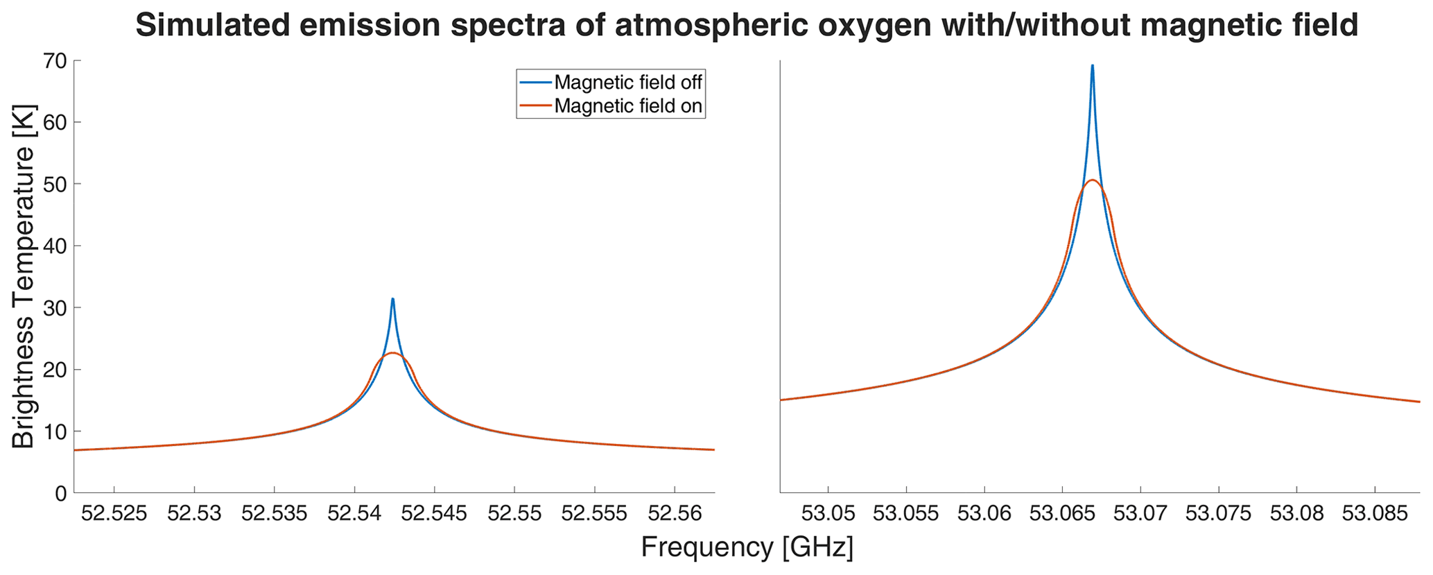
Figure 1Illustration of the Zeeman effect on the line shape for mid-latitude observations on Earth. The line of sight is directed northwards with a zenith angle of 30∘. The tropospheric effect on the brightness temperature has been removed.
Stratospheric and mesospheric temperatures obtained from the new retrieval algorithm are compared to MERRA2 reanalysis (Gelaro et al., 2017) and to the meteorological analysis NAVGEM-HA (Eckermann et al., 2018). The vertical temperature profiles are extracted for the location of Payerne considering the spatial averaging of the radiometer of about 250 km in diameter keeping the temporal resolution of the model fields of 3 h. Only the vertical resolution of the model data was interpolated to a fixed altitude grid with 2 km vertical resolution to simplify the comparisons. MERRA2 reanalysis utilizes a 3DVAR data assimilation (e.g., Gelaro et al., 2017, and references therein), which updates the state vector every 6 h. A detailed description of the hybrid 4-DVAR data assimilation in NAVGEM-HA is provided in Kuhl et al. (2013) and Eckermann et al. (2018). Similarly to MERRA2 the model state vector is updated every 6 h at the mesosphere.
For the comparison with the temperature observations from TEMPERA, the model data was analyzed at the geographic location of Payerne, and all grid points in a 250 km radius were averaged after they had been interpolated to a geometric vertical altitude grid. Daily mean temperatures and tidal amplitudes were derived by an adaptive spectral filter similarly to Pokhotelov et al. (2018), Baumgarten and Stober (2019), and Stober et al. (2020). The geopotential altitudes from NAVGEM-HA were converted into geometric heights (Stober et al., 2021). The temporal resolution of 3 h for both model data was kept.
5.1 Temperature retrievals
The inversion of the forward model is solved with ARTS 2.4 (Atmospheric Radiative Transfer Simulator; Buehler et al., 2018). The mathematical method follows the formalism from Rodgers (2000) and is briefly explained in this section.
Lets be y the measurement vector and x the state vector. In our case, y is the spectrum with n channels, and x is the temperature profile with m grid points. The forward model F(x,b) maps the atmospheric state x to an idealized spectrum, this is usually written as
The vector b contains some other parameters that are not included in the state vector, and ϵ is the measurement error. The challenge is to find an inversion of the forward model F(x,b) that presents an optimal estimate to the observations. The problem is that there is often no unique state x for a given measurement y, which is classified as ill-posed. The inversion (also called retrieval) can be understood as a mapping R of the measurement vector y onto an optimal state vector
where is the best estimate of the forward model parameters, xa denotes the a priori knowledge on the state vector, and c are some additional parameters. The optimal estimation method (OEM) provides the most probable solution in the context of the forward model. To apply this method information about the atmospheric state must be added. This information is included in the a priori state xa, which is a preknowledge background state of the atmosphere. The choice of a certain a priori state is crucial and explained in Sect. 5.2. The error covariance of the a priori state is described in the a priori-covariance matrix Sa, and the measurements errors are described in the measurement-error covariance matrix Sϵ. The optimal solution can be found by maximizing the probability P(x|y) of x under the condition that y is known, or in this case equivalent and most common, minimizing the cost function , which can be written in the form
The derivation of this cost function is based on Bayes' probability theorem, and the assumption that the probability distributions for the a priori covariance Sa and for Sϵ, as well as the posterior distribution x, are Gaussian. The minimum of J(x) is found by the following condition
This equation is solved using several iterations making use of the Levenberg–Marquardt solver. Thus, successive iterations are computed from
where is called the weighting function. The a priori profile was used for the 0th step x0=xa. For γ=0, this method is equivalent to the Gauss–Newton method. The damping term γD ensures the iteration to converge, even under poor conditions, making this method more robust but also slower compared to the Gauss–Newton scheme.
5.2 A priori atmospheric information
The retrieval algorithm is initialized using an ECMWF climatology. The climatology was obtained averaging daily mean ECMWF data between 2014–2017 smoothed by a 30 d running window. The resulting seasonal a priori temperature behavior is shown in Fig. 2. Based on this climatological mean atmospheric state, the radiative transfer equations are solved for several molecular species, e.g., O2, H2O, O3, and N2. However, not all of them contribute significantly to the radiation intensity between 50–60 GHz. Spectroscopic data for O2 was taken from the HITRAN database (Gordon et al., 2017). These quantum numbers are necessary to account for the Zeeman effect in the radiative transfer model. The magnetic field strength for the location of Bern at the altitude of the mesosphere is taken from ARTS.
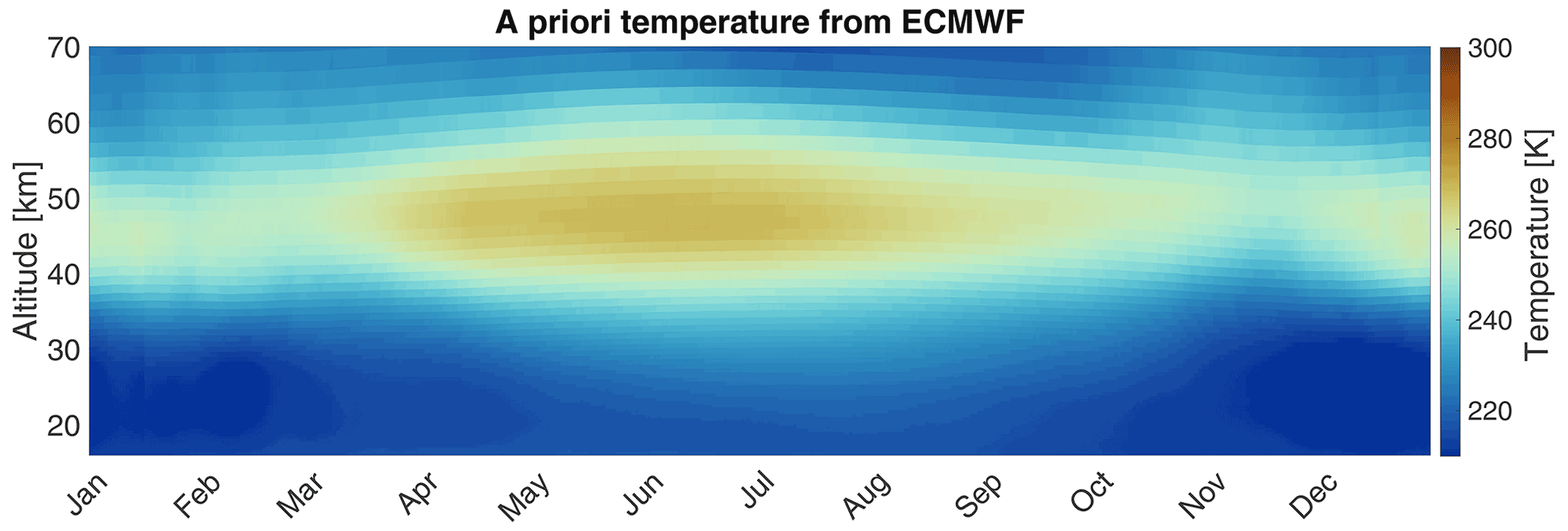
Figure 2Averaged ECMWF temperature profiles for the geolocation of Payerne (CH). A moving window of 31 d was used for smoothing after the average over the 4 years 2014–2017 was taken.
5.3 Tropospheric correction
The new retrieval still incorporates a tropospheric correction. The received signal is the integral along the line of sight of all emitted microwave radiation, also including tropospheric altitudes. However, the main goal of the new retrieval is the improvement of the stratospheric and mesospheric temperature soundings, which requires a higher frequency resolution in the line center at the cost of the much broader tropospheric signal, which still dominates the overall brightness temperature in the line wings and the center. Therefore, the tropospheric signal is separated and removed from the stratospheric and mesospheric intensities by implementing a tropospheric correction. The method is based on the assumption that the troposphere can be approximated by a homogeneous layer with a weighted mean brightness temperature
Where the integral is taken from the ground z1 to the top of the troposphere zt, ν is the frequency, α denotes the absorbing coefficient, τ the opacity, and T(z) is the physical thermal equilibrium temperature. The weighted mean temperature is used to estimate a mean tropospheric opacity τtrop(ν). After estimating all these parameters the brightness temperature on the top of the troposphere is determined by solving the radiative transfer equation. The integrals above are dominated by the lowest altitudes because α is pressure dependent and decreases quickly with increasing altitude. Assuming a linear relationship between the surface temperature Ts and Tm leads to
To determine the coefficients a and b radiosonde measurements at Payerne launched from MeteoSwiss were used. The coefficients for the TEMPERA frequency range are found in Navas-Guzmán et al. (2015) and take values for a=0.8159 and b=47.211. Further details about the method are described in Ingold and Kämpfer (1998). All previous studies based on TEMPERA have applied such a tropospheric correction (Stähli et al., 2013; Navas-Guzmán et al., 2015, 2017). Although, hitherto observations with TEMPERA indicate that the tropospheric correction seems to work well, it represents a coarse approximation that is worth further investigation for various weather conditions. In particular, tropospheric inversion layers might have a more critical impact on the mean tropospheric opacity τtrop(ν).
5.4 Measurement errors
Statistical measurement errors arise from two sources. The first error source is the receiver noise and the second one is atmospheric noise, which originates from fluctuations and turbulent processes in the field of view. Typically, receiver and atmospheric noise are considered as zero-mean Gaussian random processes. Both together, measurement-noise-variance and atmospheric-noise-variance contribute to the measurement-error covariance (Rodgers, 2000). Other systematic errors, such as a systematic frequency shift in the channels, are often hard to identify and, thus, are not taken into account.
In the following, we briefly discuss how the measurement errors are obtained. Considering as the measurement matrix, νi is the frequency of channel number i, and tj is the time of spectrum number j in a time series with N spectra. The channels are assumed to be uncorrelated with the variance . The final measurement spectrum is the mean of yij over time , so that the variance of is related to as
From this, one can calculate by taking the sample variance of . A more stable method is to consider the variance of the differences , which is related to σi as and, hence,
Assuming that all channels are uncorrelated, the measurement error covariance matrix Sϵ takes a diagonal form with entries
5.5 A priori covariance
The a priori covariance determines the uncertainty of the a priori state. For temperature profiles, one usually chooses a constant value for each grid point and a with distance exponentially decreasing correlation. However, varying the a priori covariance with altitude can improve the retrieval significantly with respect to the measurement response obtained. Since the platform altitude was set at 12 km (see tropospheric correction), lower altitudes have to be excluded from the inversion. For this purpose, the a priori covariance σa(zi) was set to 0.1 K up to 12 km (zi is the altitude at the ith grid point). Above the virtual platform altitude, the a priori covariance increases linearly with altitude to a value of 6 K at 50 km, and higher up in the atmosphere, the value increases to 8 K at 60 km and beyond that height, the covariance reaches 12 K at 70 km altitude. A linear increase with altitude avoids numerical oscillations due to sharp “jumps” in the profile, which would occur when a step function is implemented instead. The larger values at the upper altitudes of the retrieval domain are beneficial to optimize the information content of the measurement vector. However, we have to note that this method tends to be more prone to generate some unwanted numerical effects such as spurious oscillations. On the other hand, a smaller choice of the a priori covariance for these altitudes forces the retrieval to stay close to the a priori state, and, thus, information content would be lost. The values described above were optimized through empirical tests prioritizing an optimal balance between numerical stability and high sensitivity of the solution at the stratosphere and lower mesosphere. Considering these aspects, the covariance matrix Sa takes the form
where h is the correlation length, which was set to be h=1 km.
5.6 Other sources of uncertainty
The advantage of the optimal estimation implementation of the retrieval is the possibility to derive the information gain from the observations (Shannon, 1948; Shannon and Weaver, 1949). An important quantity, which is widely used for error analysis in information theory, is the gain matrix given by
The gain matrix can be interpreted as the sensitivity of the retrieval R to the measurement y. Furthermore, the gain matrix can be used to define the averaging kernel matrix by
According to Rodgers (2000) the averaging kernel is the sensitivity of the retrieval to the (unknown) true state. The rows of A provide correlations and a distinct maximum, which defines the altitude of maximum measurement response for a vertical grid point. Their half-width can be regarded as a measure of the effective vertical resolution. The measurement response vector mr is defined as (Rodgers, 2000; Eriksson et al., 2005)
where Ai is row i of the averaging kernel matrix, and xai is the ith entry of the a priori state. For an ideal retrieval, the value of mr equals 1. The lower the measurement response, the more a priori information is included in the solution. Measurement responses below 0.6 indicate that the retrieved state depends mostly on our a priori information.
Weighting the measurement-error covariance matrix Sϵ with Gy one obtains the retrieval noise (or observational error) covariance matrix
Another indicator is the modeling error sM, obtained by weighting the retrieval residuals with Gy
In theory, this vector should be evaluated at the true state x and b, which is, of course, not known. Evaluating this quantity at the retrieved state instead will lead to slightly increased values.

Figure 3Different error components from the retrieval method (a). Units of errors are always Kelvin here. Measurement response (MR) and averaging kernel matrix (AVK) (b). The AVK is multiplied by a factor of 10 for a facilitated comparison with the MR.
As an example, a set of quality control parameters are illustrated in Fig. 3. The modeling error, which is directly related to the forward model residuum, leads to the conclusion that the retrieved profile is underestimated around 30–40 km and overestimated around 45–55 km by about 2 K.
The AVK up to 40 km shows the expected and already documented behavior (Stähli et al., 2013; Navas-Guzmán et al., 2017), where the best performance is reached at an altitude around 30 km. From 40 km upwards the Zeeman calculation leads to a second but lower peak between 40–50 km. The last peak between 60–65 km is due to the increased a priori error in this region. This behavior is also reflected in the measurement response. As a rule of thumb, the altitude range of a retrieved profile is usually defined as the region where the measurement response is above 0.8, which can be found at altitudes between 22–53 km.
The revised temperature retrieval was applied to data collected with TEMPERA in Payerne between 2014–2017. The main differences compared to previous work by Navas-Guzmán et al. (2015, 2017) is the inclusion of the Zeeman effect in the center of the oxygen emission lines and the use of updated a priori and measurement covariances to improve numerical stability and the retrieval sensitivity. Furthermore, there is the new retrieval emphasis on stratospheric and mesospheric altitudes to observe tidal waves and their temporal intermittency. The temporal resolution was slightly decreased from 2 h (Navas-Guzmán et al., 2017) to about 2.5 h. The increased integration time resulted in more robust temperature estimates. On average, we obtained 8–9 integrated spectra per day. Each integrated spectra consists of about 150–160 individual atmospheric soundings and spectra obtained from atmospheric observations lasting 0.5 s (mirror pointing towards sky) using the stratospheric and mesospheric measurement mode with the high-resolution FFT-spectrometer.
We also implemented a quality control before the averaged spectra is computed. Some spectra are removed from the averaging due to increased atmospheric noise, mainly caused by tropospheric weather, e.g., strong precipitation or temporary technical issues with the instrument. On average, about 3.6 % of the integrated spectra are removed from the analysis within the 4 years of observations.

Figure 4Continuous atmospheric temperature profiles, retrieved from TEMPERA measurements in comparison to MERRA2 and NAVGEM-HA data for the years 2014–2017 over the geolocation of Bern (CH). The altitude range is 53 km. Above 53 km the retrieved profiles are dominated by the a priori profiles.
Figure 4 shows temperature soundings for TEMPERA, MERRA2, and NAVGEM-HA for the whole period (2014–2017). The seasonal pattern indicates higher temperatures at all retrieved altitudes during the summer season and lower temperatures at the stratosphere during the winter months. The winter months are characterized by an increased planetary wave activity and the frequent occurrence of sudden-stratospheric-warmings (Scherhag, 1952; Matsuno, 1971; Limpasuvan et al., 2016; Matthias et al., 2013). Also, the spring transition is clearly distinguishable from the temperature data (Matthias et al., 2021).
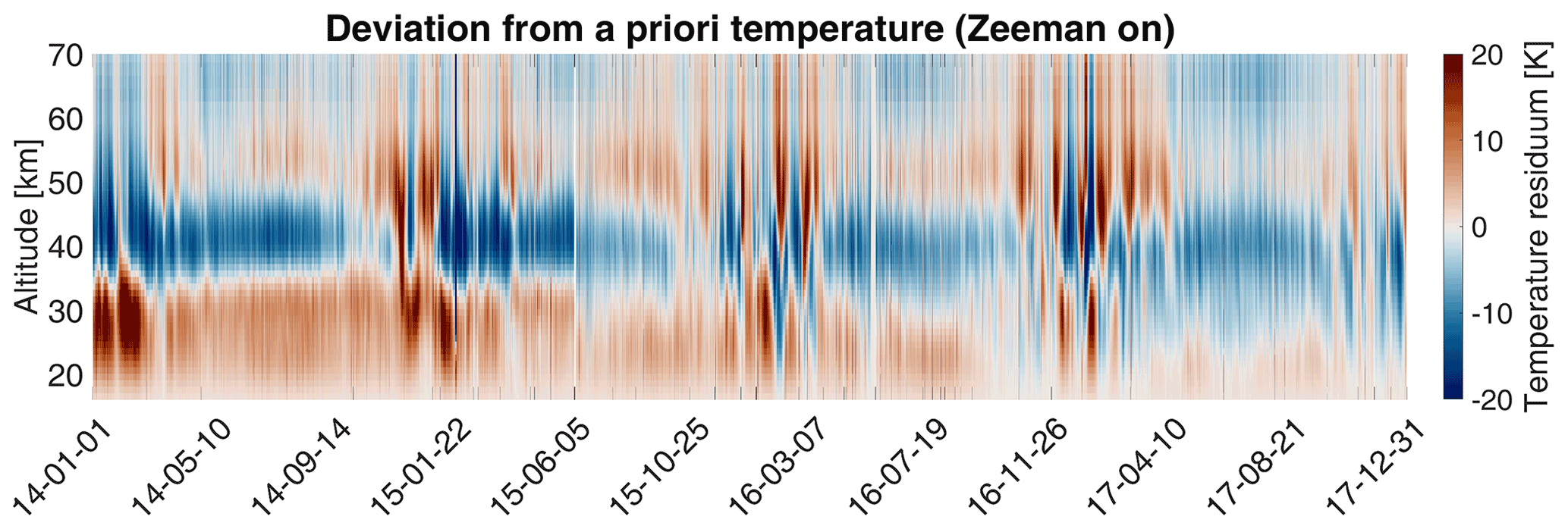
Figure 5Absolute differences between retrieved TEMPERA profiles and a priori profiles. Reddish regions indicate higher values for the retrieved quantities in comparison to the a priori ones. Bluish areas support colder temperatures concerning the a priori state.
First of all, we investigated how critically the final retrieved temperatures depend on our a priori data. Figure 5 shows a difference between TEMPERA and the ECMWF climatology. The larger the differences at some altitudes, the less critical is the choice of the a priori data, which indicates that at these levels, the solution is only given by the measurements. Furthermore, from 60 km and higher up, the colors become brighter, which points out that these heights depend more on the a priori information. This is also reflected by the lower measurement response and is consistent with the averaging kernels presented in Fig. 3 for these altitudes.
The performance of the new temperature retrievals is assessed by comparing our observations to state-of-art reanalysis data from MERRA2 and the meteorological analysis of NAVGEM-HA. Therefore, we compute correlation coefficients based on monthly medians and corresponding variances for all data sets. These monthly medians essentially remove all atmospheric waves on short timescales, such as tides and gravity waves, from the model fields as well as the temperature soundings. However, we have to note that atmospheric time series cannot necessarily be considered as Gaussian random variables. Often, the atmospheric natural variability exceeds the statistical uncertainty of the observations (e.g., Stober et al., 2017, see Fig. 3), and, thus, an overestimation or inflation of the correlation coefficients is the result. Assuming a linear regression model between the TEMPERA profiles TTMP(z) and the profile for cross comparison TCCP(z)
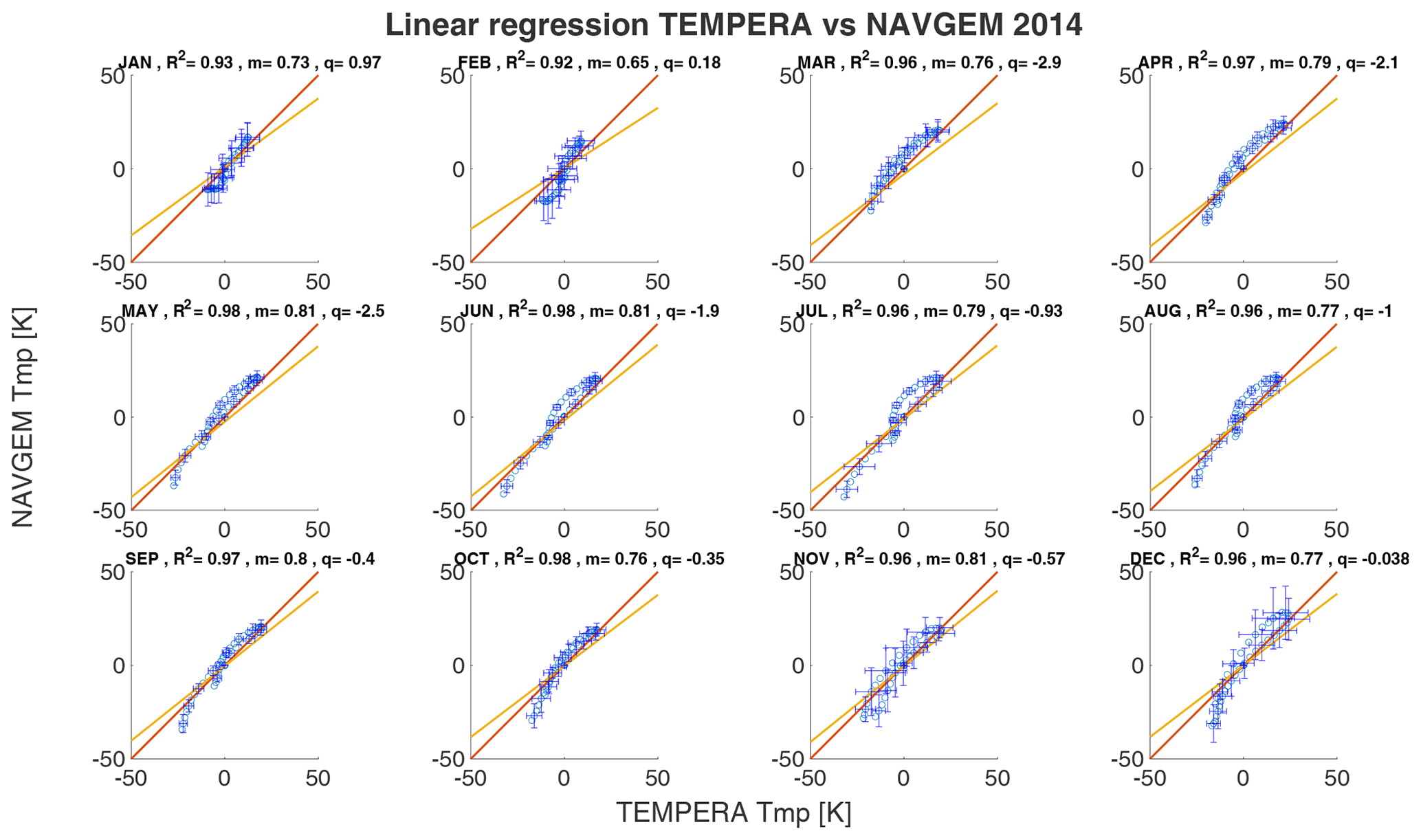
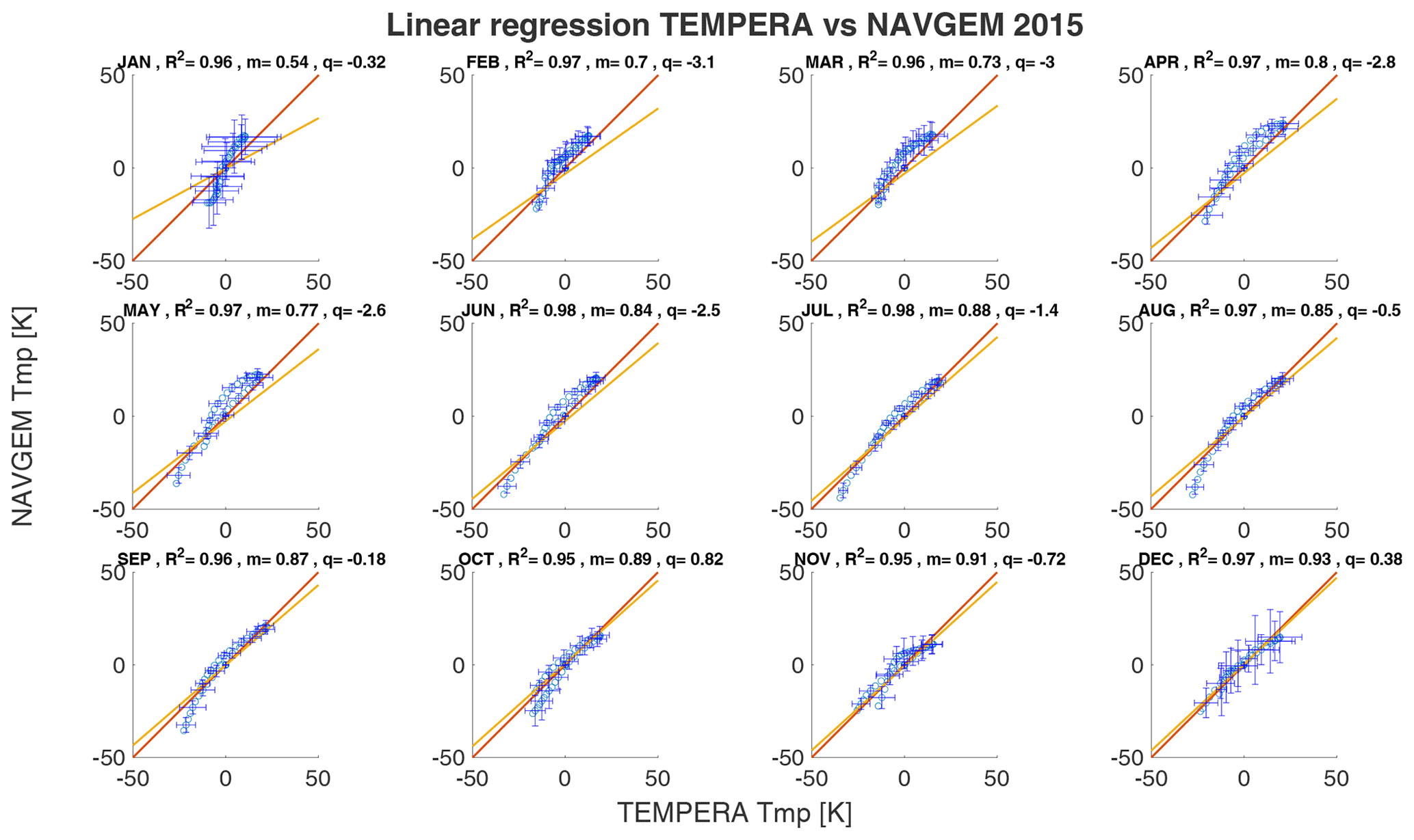
the coefficients m,q were determined through linear regression. For two statistically identical data sets, we would obtain m=1, and q=0. The coefficient q gives an absolute offset of the two profiles, while a slope m above 1 indicates a higher sensibility of the profile TTMP(z) (see Sect. 8) relative to the compared profile TCCP(z). This method gives a quantitative estimation of the absolute offset but provides no information as to at which altitude this occurs. In Figs. 6 and 7 we show linear correlation coefficients of the median monthly temperature profiles for the year 2016 for TEMPERA vs MERRA2 and TEMPERA vs. NAVGEM-HA, respectively. The error bars correspond to the temperature variance for each data set. The correlations are estimated after subtracting the median temperature from each profile, which was estimated to be approximately 250 K
The shift of the temperature profile to lower values is necessary because the linear regression would otherwise falsely give good values for m. The other years can be found in Appendix A.
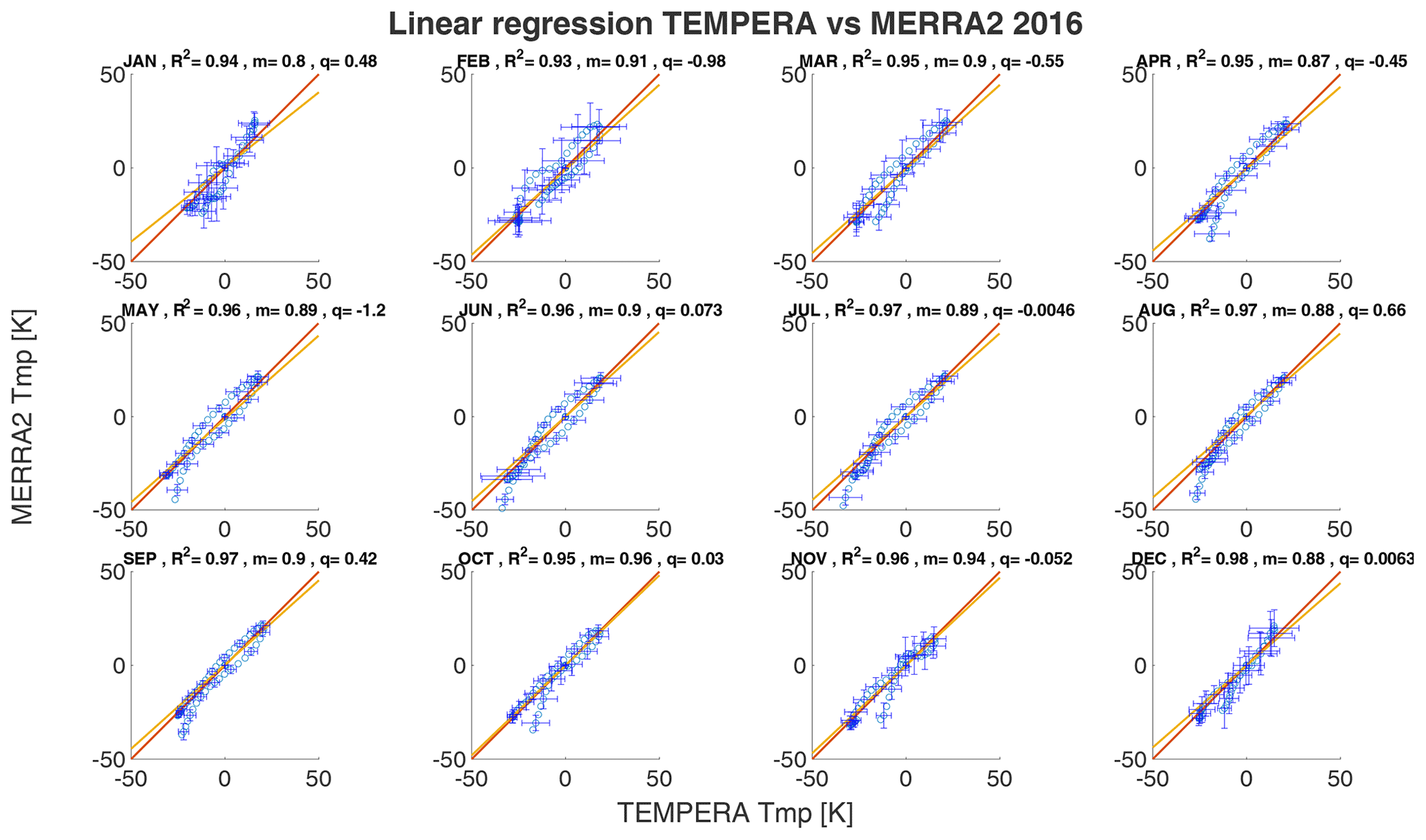
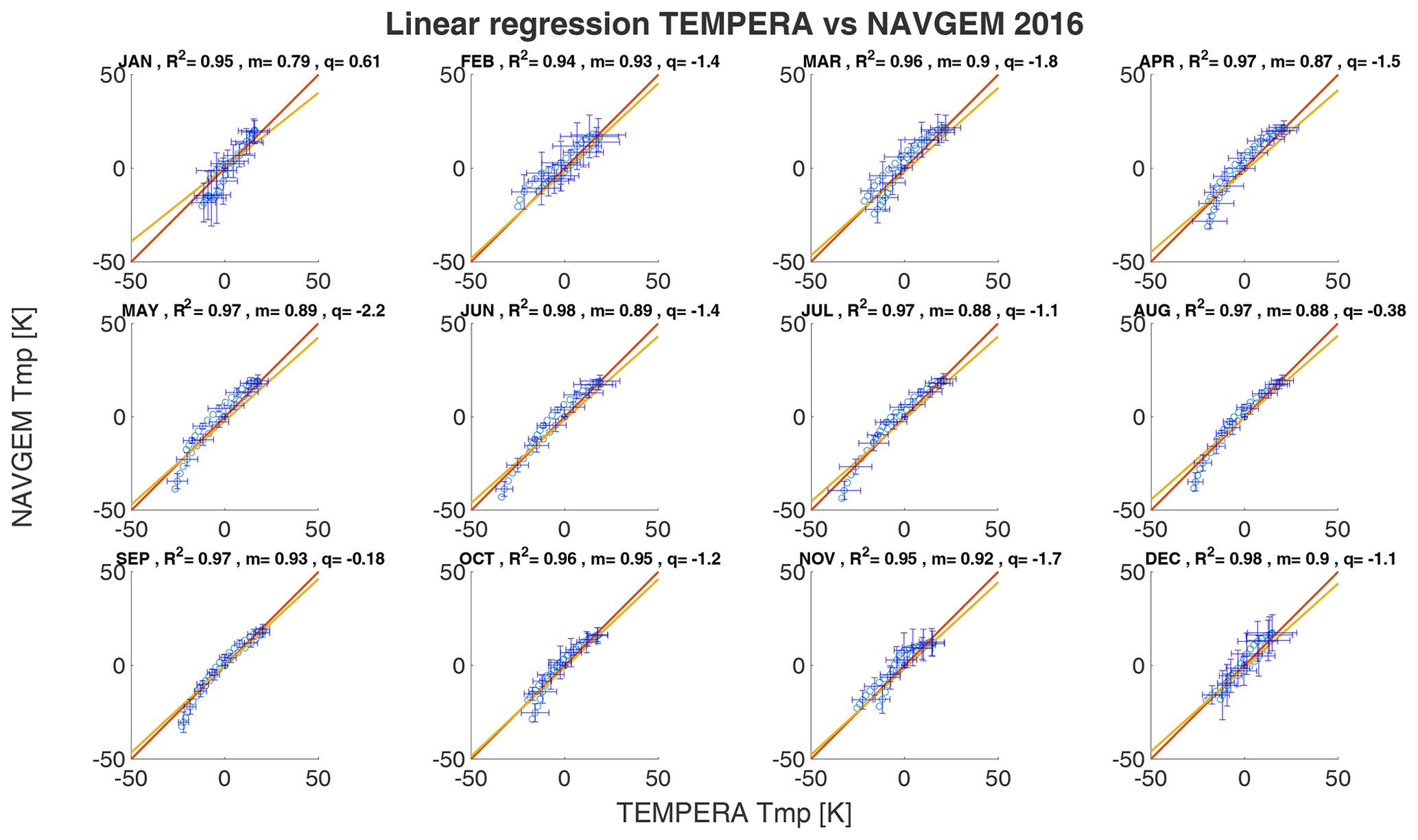
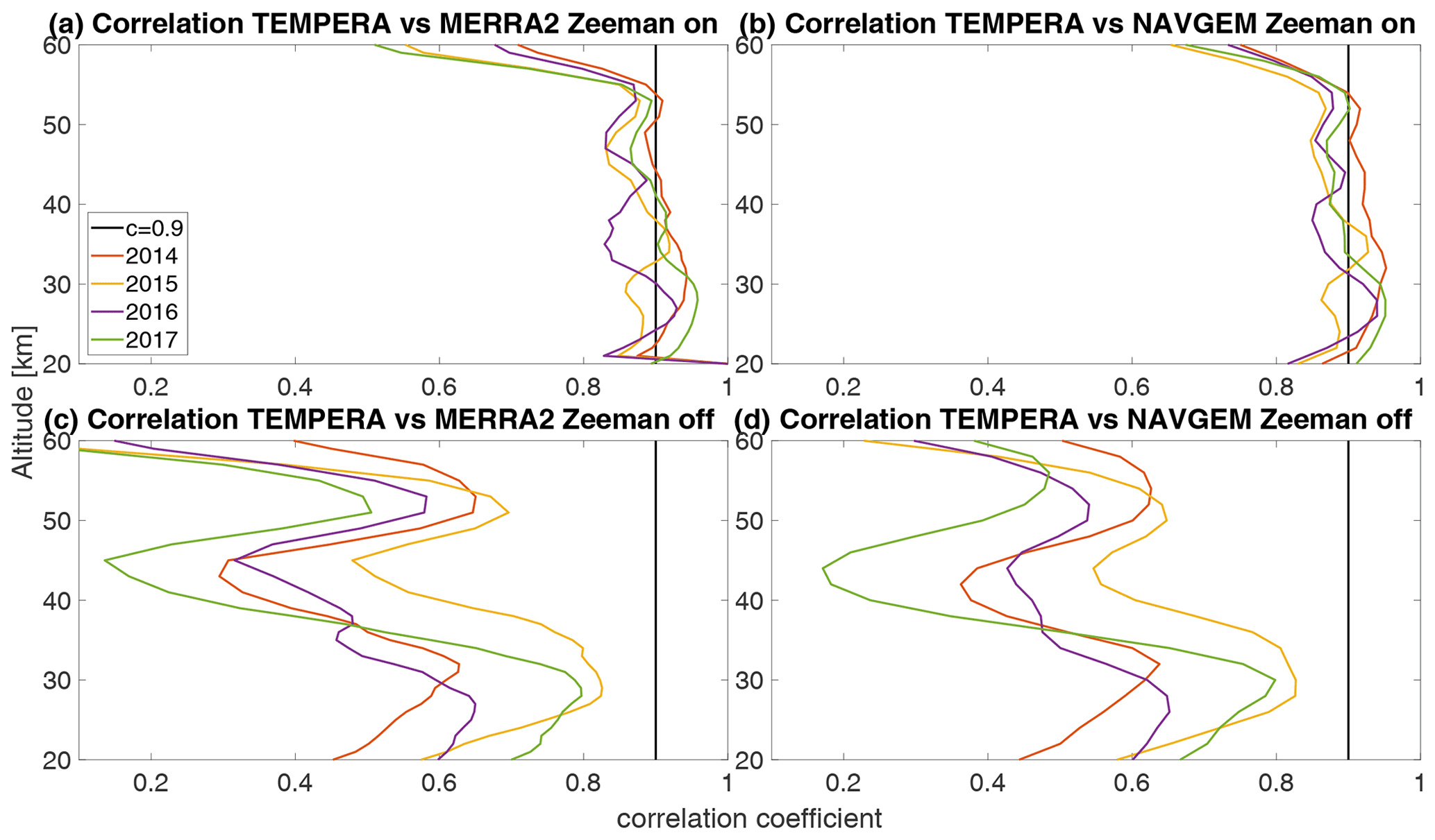
Figure 8Correlation coefficients over altitude between TEMPERA and MERRA2 data (a, c), and TEMPERA and NAVGEM-HA (b, d) data. Calculations were performed with activated Zeeman effect (a, b) and deactivated Zeeman effect but with the full line center included (c, d).
The monthly median temperature correlation coefficients exhibit a range between 0.93–0.98 for the comparison with MERRA2 and about 0.94–0.98 for NAVGEM-HA. The highest correlation coefficients are achieved during the summer months from April to September and in December. The lowest correlations are found during January and February and are the result of the increased planetary wave activity and the more variable polar vortex dynamics in 2016 (Matthias et al., 2016; Stober et al., 2017; Matthias and Ern, 2018). NAVGEM-HA indicates a similar seasonal behavior for the year 2016 and occasionally has minimal larger correlations. The mean temperature bias between the new TEMPERA retrievals and MERRA2 is smaller than 1.5 K. The temperature bias relative to NAVGEM-HA takes values between −0.1 up to −2.2 K (excluding the exceptional January 2016). The slopes m of the linear regression with MERRA2 and NAVGEM-HA are in a range between m=0.8 and m=0.96, indicating a lower sensitivity of TEMPERA to the atmospheric variability relative to the model fields. We also estimated yearly median altitude-resolved Pearson correlation coefficients. These are shown in Fig. 8. It is remarkable that the correlation coefficients for retrievals with activated Zeeman effect (upper panels) are most of the time larger than 0.8 and often exceed 0.9 for MERRA2 and NAVGEM-HA, respectively. Furthermore, the seasonal correlation coefficients reveal a sharp drop off at about 53–55 km, which appears to be the limiting altitude for TEMPERA temperatures and the new retrieval. Above this altitude, the solutions of the retrieval are dominated by a priori information. The comparison also indicates that NAVGEM-HA exhibit a slightly higher correlation concerning TEMPERA temperatures relative to MERRA2.
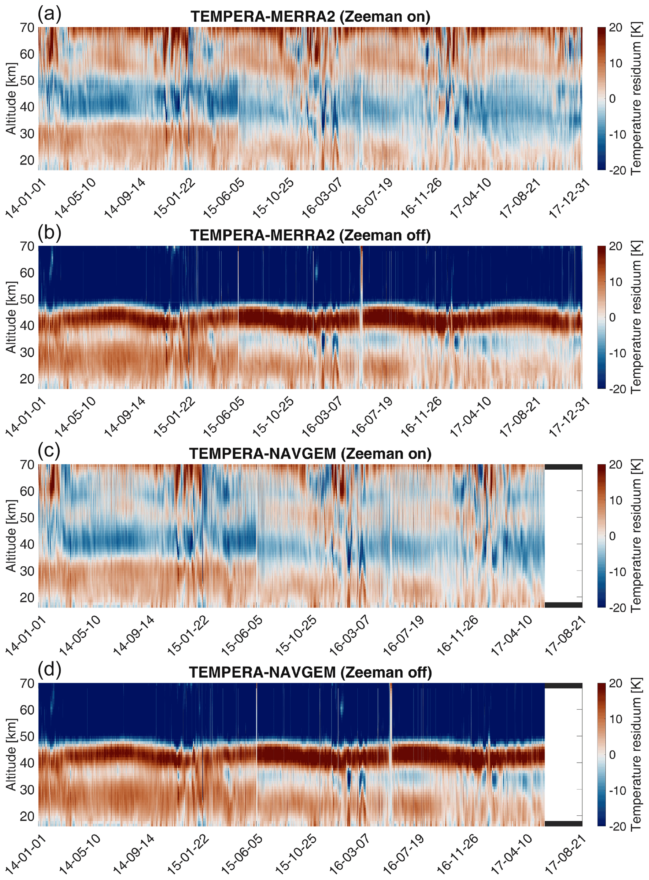
Figure 9Absolute differences between TEMPERA and MERRA2 (a, b), and NAVGEM-HA (c, d). Calculations with Zeeman off were performed including the line center in order to show the influence of the Zeeman broadening on the retrieved profile. Red regions indicates higher values of TEMPERA.
In addition, Fig. 8 (lower panels) show yearly correlation coefficients for TEMPERA retrievals with deactivated Zeeman effect. For calculations without the Zeeman effect, usually the line center is blanked and only the line wings are used. This approach results in retrievals with a limited upper altitude of about 45 km. Above this altitude, the retrieved profile quickly converges towards the a priori profile, because due to the missing line center the measurements do not provide any information beyond these heights. Besides some small effects, the profiles with activated and deactivated Zeeman effect would match up to this altitude. The plots with Zeeman on/off are shown in Figs. 8 and 9. However, we retrieved temperatures keeping the line center but turned off the Zeeman effect by setting the magnetic field essentially to zero to investigate the impact of the Zeeman broadening. Correlation coefficients for retrievals with deactivated Zeeman effect are lower than 0.9 everywhere and even lower than 0.8 for most of the altitudes. This underlines that accounting for the Zeeman effect has not only an impact on the upper altitudes. Due to the energy conservation in the radiative transfer, almost all altitudes are affected with decreasing impact for the lower altitudes.
Another important aspect to compare are altitude-time-dependent systematic differences between MERRA2 and NAVGEM-HA. Therefore, we compute altitude time residuals by subtracting MERRA2 and NAVGEM-HA from the temperatures observed by TEMPERA. Figure 9 shows the resulting temperature residuals for both model data sets and the complete time series. Similarly to the Pearson correlation coefficients MERRA2 and NAVGEM-HA reflect the same characteristic systematic differences. Furthermore, the installation and upgrade of the receiver around 5 June 2015 is clearly visible in the residual comparison. The new receiver reduced the standing wave contamination in the line wings and, thus, mostly affected the data quality below 40 km altitude.
In addition, Fig. 9 shows difference plots for TEMPERA retrievals with deactivated Zeeman effect and the full line center (the same as Fig. 8).
The vertical residuals show some systematic and altitude-dependent differences. Below 35 km there is a tendency for TEMPERA to show warmer temperatures compared to MERRA2 and NVAGEM-HA. Between 35–50, the models seem to have a warm bias compared to the radiometric temperature sounding. Above 53 km MERRA2 indicates a clear tendency to underestimate the temperatures relative to TEMPERA, whereas NAVGEM-HA shows a more variable vertical structure of the residual temperature exhibiting times and altitudes with warmer, but also periods and heights with colder temperatures. It is also evident from the residual comparison that during the winter season the increased planetary wave activity leads to larger differences between our temperature observations and the model data.
The plots with Zeeman effect turned off shows cold biases of 20 K above 45 km and hot biases around 5–20 K below. The cold bias is due to an overestimation of the pressure broadening since the Zeeman broadening is treated as pressure broadening when Zeeman calculations are deactivated. Hot biases occur mainly as an effect of compensation since the total radiation intensity along the beam path has to be preserved.
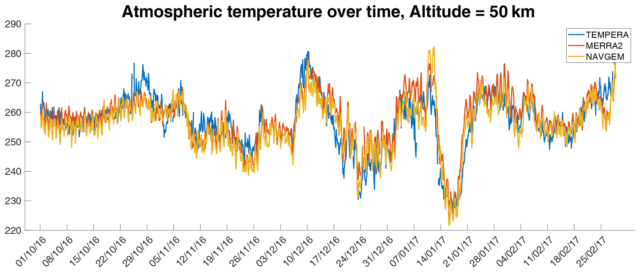
Figure 10Comparison of TEMPERA, MERRA2, and NAVGEM temperatures on a larger timescale (months), at which planetary waves occur, and a smaller timescale (days), which is the timescale of atmospheric tides.
Finally, Fig. 10 presents a comparison of the 3-hourly resolved temperature time series at 50 km altitude. The comparison underlines that the TEMPERA observations still exhibit such a high measurement response at this height that the temperature amplitude and phase of planetary waves is well captured in comparison to MERRA2 and NAVGEM-HA. There is also a characteristic diurnal tidal oscillation in MERRA2, NAVGEM-HA, and the radiometer data visible. Overall the measurements from TEMPERA and the MERRA2 and NAVGEM-HA temperature agree within a few kelvin (5–10 K). Furthermore, the comparison supports that it is feasible to obtain tidal information from the TEMPERA temperature soundings on a daily basis.
The main goal of the new retrieval algorithm was the implementation of the Zeeman effect in the temperature retrievals, which was not available in previous versions of the radiative transfer model for both oxygen emission lines. Thus, the new temperature retrieval yields an increased measurement response and altitude coverage up to 55 km compared to former TEMPERA observations where 45–48 km seemed to be the limiting altitude (Stähli et al., 2013; Navas-Guzmán et al., 2015). Furthermore, the new retrieval was optimized concerning the a priori state vector and covariances, which also led to some improvement at the upper stratosphere and lower mesospheric heights. TEMPERA observations offer the possibility to perform continuous temperature measurements at altitudes between 16–55 km.
While implementing a new retrieval method it is always necessary to achieve a balance between numerical stability and sensitivity to the atmospheric state. A small a priori covariance or a too large measurement error results in low sensitivity of the retrieval, although such a retrieval is stable concerning numerical oscillations. On the other hand, such a retrieval likely underestimates the natural or true variability of the estimated parameters, and the solution would stay tied to the a priori state. A large a priori covariance improves the sensitivity of the retrieval, but at the cost of numerical oscillations, which can dominate the whole retrieved profile. The new retrieval is well balanced to achieve the highest possible sensitivity at 50 km while avoiding numerical instabilities and oscillations.
Statistical measurement errors are known with high precision; the final error on the temperature profile is rather a measure of the information content rather than an error in the classical sense. The state-of-the-art method is a cross comparison of different and independent data sets. Calculations of correlation coefficients or goodness-of-fit values (R2) in a linear regression always requires some information about the uncertainty of the data set. Since this information is missed, usually the sample variation is taken instead. This approach should, however, be used with appropriate caution because atmospheric profiles or time series are not random variables, and natural variations could be bigger than the actual errors. This circumstance leads directly to an overestimation of the correlation coefficients of two compared data sets.
Continuous temperature observations at the stratosphere and mesosphere are rare. Lidars are often limited by the tropospheric weather conditions, and only a few long observations are available (e.g., Stober et al., 2017; Baumgarten and Stober, 2019; Eixmann et al., 2020). However, these lidar studies underline that continuous temperature observations are essential to investigate atmospheric wave and their intermittency covering periods from gravity waves, tides, and planetary waves at the source region, to research wave–wave interactions.
Satellite observations from MLS or SABER provide neither the temporal nor the spatial resolution to resolve all atmospheric waves and their intermittent behavior. Due to the spacecraft orbit and viewing geometry very often only one measurement per day is available for a specific geographic location. However, satellite observations are a key information source for data assimilation into MERRA2 and NAVGEM-HA at the stratosphere and mesosphere for the temperature and dynamical fields (Gelaro et al., 2017; Kuhl et al., 2013; Eckermann et al., 2018). Other meteorological observations such as radiosondes reach only altitudes of about 28–38 km and, thus, provide only temperature, wind, or chemical information at the lower and middle stratosphere. Furthermore, radiosondes are launched every 12 h, or at some stations occasionally every 6 h, which limits their impact to capture atmospheric tides at the stratosphere.
Navas-Guzmán et al. (2017) has already performed an intercomparison of the TEMPERA observations with MLS satellite data, lidar, and radiosondes, as well as WACCM simulations. The Pearson correlation coefficients obtained were between 0.9 to 0.94 for a 3-year-long time series and were interpolated to match the different temporal resolutions and emphasized altitudes between 22–43 km where the measurement response was larger than 0.8. In this study, we have already achieved this degree of correlation using median monthly profiles and for yearly observations for the altitude range from 20–55 km. However, the comparison to MERRA2 and NAVGEM-HA still exhibits a warm bias of TEMPERA for the altitude range between 20–30 and 35 km and a cold bias between 30(35)–48 km, which was already found in Navas-Guzmán et al. (2017). Some of the systematic biases at the lower altitudes as well as at the upper altitudes occur at heights with a low measurement response, and thus we investigated a potential a priori dependence by computing similar climatologies for MERRA2 and NAVGEM-HA as shown in Fig. 2 for ECMWF. A comparison of these a priori climatologies between all three reanalysis data sets revealed similar altitude-dependent offsets to the TEMPERA comparison and explains most of the upper stratospheric bias and at least partly the lower stratospheric offset.
In this study, we reprocessed observations of the TEMPERA radiometer conducted between 2014 and 2017 with a recently developed and updated temperature retrieval. The new algorithm accounts for the Zeeman effect in the line center for both oxygen emission lines and uses revised a priori information for the state vector and covariances. We demonstrate with the new retrievals that TEMPERA temperature soundings can be carried out nearly continuously and with an increased altitude coverage by leveraging the updated radiative transfer model (ARTS) and HITRAN quantum numbers, which were not available previously.
We validated the retrieved temperature against the MERRA2 reanalysis and the meteorological analysis NAVGEM-HA for the years 2014–2017. Seasonal Person correlations coefficients remained between 0.85–0.95 between 20–55 km altitude. Therefore, we conclude that considering the Zeeman effect in the line center together with the revised a priori information resulted in an extended altitude coverage of about 8–10 km compared to the previous algorithm applied to the same TEMPERA measurements while sustaining the temporal resolution (Stähli et al., 2013; Navas-Guzmán et al., 2017).
Furthermore, we assessed the correlation coefficients and mean biases for monthly median temperature profiles of TEMPERA and the validation data MERRA2 and NAVGEM-HA. We obtained correlation values between 0.8–0.96 throughout the course of the year. The smallest correlations are found in January and February during strong planetary wave activity or for stratospheric warming evens, which supports that high-quality local observations could still provide a benefit to studying dynamical processes in more detail. The months from April to September reached correlations between 0.94–0.96. The mean temperature bias between MERRA2 and the radiometric temperatures was smaller than ±1 K and basically vanished for some months. However, the comparison to NAVGEM-HA resulted in a cold bias between 1–2 K for the TEMPERA temperatures.
Altitude-dependent differences were examined by computing temperature residuals of TEMPERA and both model data sets. We identified that the lower altitudes between 20–35 km tend to exhibit a warm bias of approximately 5 K for the radiometer, and from 35–50 km we found a systematic cold bias of approximately 5 K for TEMPERA compared to MERRA2 and NAVGEM-HA. Above 50 km altitude, MERRA2 and NAVGEM-HA also start to show some discrepancies in the vertical temperature structure. During strong planetary wave activity in the winter months the differences between MERRA2, NAVGEM-HA, and TEMPERA exceed ±10 K. However, it remains unclear whether these biases or differences are due to the instrument or due to the sparsity of the assimilated data in the models, which might be not sufficient to capture all dynamical details.


In Fig. B1 we show a differences between MERRA2 and NAVGEM-HA. Both models exhibit a very good agreement up to an altitude of 53 km. Above 53 km a systematic difference is obvious. NAVGEM-HA tends to show larger temperatures compared to MERRA2. However, we did not investigate the nature for the increasing discrepancy between both models above this altitude, which is beyond the scope of the paper. A detailed overview of the assimilated data sets and altitude range can be found in Eckermann et al. (2018) for NAVGEM-HA and for MERRA2 in Gelaro et al. (2017).
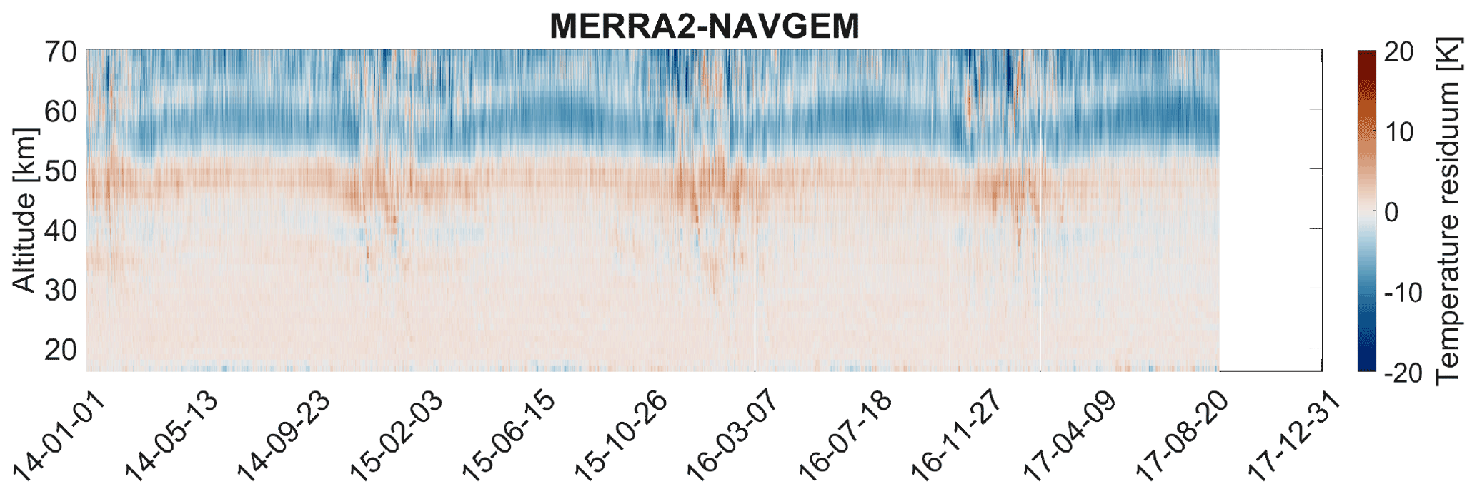
Figure B1Absolute temperature difference between the MERRA2 and NAVGEM-HA datasets shows seasonal patterns above 45 km. The color scale is the same as in Fig. 9.
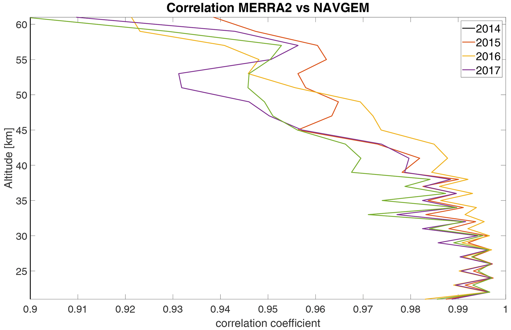
Figure B2Correlation coefficients between the MERRA2 and NAVGEM-HA datasets. Correlation coefficients over all altitudes are above 0.9.
MERRA-2 data are available at MDISC, managed by the NASA Goddard Earth Sciences (GES) Data and Information Services Center (DISC) https://doi.org/10.5067/QBZ6MG944HW0 (GMAO, 2015). TEMPERA temperatures are shared on request (gunter.stober@unibe.ch). The NAVGEM-HA data is available upon request from NRL (https://map.nrl.navy.mil/map/pub/nrl/navgem/, last access: 11 April 2022).
WK and GS conceptualized the content of the manuscript. WK implemented the retrieval and performed the data analysis of TEMPERA observations. GS reduced the MERRA2 and NAVGEM-HA data for the validation. AM, FNG, and DK guided and supported the preparation of the paper. All authors contributed to the editing of the paper.
The contact author has declared that neither they nor their coauthors have any competing interests
Publisher’s note: Copernicus Publications remains neutral with regard to jurisdictional claims in published maps and institutional affiliations.
The authors acknowledge the European Centre for Medium-Range Weather Forecasts (ECMWF) for the data supplied. This research has been supported by the Schweizerischer Nationalfonds zur Förderung der Wissenschaftlichen Forschung (grant no. 200021-200517/1), and the Swiss Polar Institute (SPI) supports the development of the TEMPERA-C radiometer. Francisco Navas-Guzmán received funding from the Ramon y Cajal program (ref. RYC2019-027519-I) of the Spanish Ministry of Science and Innovation. We thank the ARTS developer team for their support in implementing the Zeeman effect into the retrievals. Scientific color maps (Crameri et al., 2020) are used in this study to prevent visual distortion of the data and exclusion of readers with color-vision deficiencies.
This research has been supported by the Schweizerischer Nationalfonds zur Förderung der Wissenschaftlichen Forschung (grant no. 200021-200517/1), Swiss Polar Institute (SPI), and Ramon y Cajal program of the Spanish Ministry of Science and Innovation (grant no. RYC2019-027519-I).
This paper was edited by Christian von Savigny and reviewed by two anonymous referees.
Anderson, J. G., Weisenstein, D. K., Bowman, K. P., Homeyer, C. R., Smith, J. B., Wilmouth, D. M., Sayres, D. S., Klobas, J. E., Leroy, S. S., Dykema, J. A., and Wofsy, S. C.: Stratospheric ozone over the United States in summer linked to observations of convection and temperature via chlorine and bromine catalysis, P. Natl. Acad. Sci. USA, 114, E4905–E4913, https://doi.org/10.1073/pnas.1619318114, 2017. a
Baumgarten, K. and Stober, G.: On the evaluation of the phase relation between temperature and wind tides based on ground-based measurements and reanalysis data in the middle atmosphere, Ann. Geophys., 37, 581–602, https://doi.org/10.5194/angeo-37-581-2019, 2019. a, b, c
Baumgarten, K., Gerding, M., Baumgarten, G., and Lübken, F.-J.: Temporal variability of tidal and gravity waves during a record long 10-day continuous lidar sounding, Atmos. Chem. Phys., 18, 371–384, https://doi.org/10.5194/acp-18-371-2018, 2018. a
Buehler, S. A., Mendrok, J., Eriksson, P., Perrin, A., Larsson, R., and Lemke, O.: ARTS, the Atmospheric Radiative Transfer Simulator – version 2.2, the planetary toolbox edition, Geosci. Model Dev., 11, 1537–1556, https://doi.org/10.5194/gmd-11-1537-2018, 2018. a, b, c
Crameri, F., Shephard, G. E., and Heron, P.: The misuse of colour in science communication, Nat. Commun., 11, 5444, https://doi.org/10.1038/s41467-020-19160-7, 2020. a
Dhadly, M. S., Emmert, J. T., Drob, D. P., McCormack, J. P., and Niciejewski, R. J.: Short-Term and Interannual Variations of Migrating Diurnal and Semidiurnal Tides in the Mesosphere and Lower Thermosphere, J. Geophys. Res.-Space, 123, 7106–7123, https://doi.org/10.1029/2018JA025748, 2018. a
Eckermann, S. D., Ma, J., Hoppel, K. W., Kuhl, D. D., Allen, D. R., Doyle, J. A., Viner, K. C., Ruston, B. C., Baker, N. L., Swadley, S. D., Whitcomb, T. R., Reynolds, C. A., Xu, L., Kaifler, N., Kaifler, B., Reid, I. M., Murphy, D. J., and Love, P. T.: High-Altitude (0-100 km) Global Atmospheric Reanalysis System: Description and Application to the 2014 Austral Winter of the Deep Propagating Gravity Wave Experiment (DEEPWAVE), Mon. Weather Rev., 146, 2639–2666, https://doi.org/10.1175/MWR-D-17-0386.1, 2018. a, b, c, d, e
Eixmann, R., Matthias, V., Höffner, J., Baumgarten, G., and Gerding, M.: Local stratopause temperature variabilities and their embedding in the global context, Ann. Geophys., 38, 373–383, https://doi.org/10.5194/angeo-38-373-2020, 2020. a
Eriksson, P., c. Jiménez, and Buehler, S.: Qpack, a general tool for instrument simulation and retrieval work, J. Quant. Spectrosc. Ra., 91, 47–64, 2005. a, b, c
Gelaro, R., McCarty, W., Suárez, M. J., Todling, R., Molod, A., Takacs, L., Randles, C. A., Darmenov, A., Bosilovich, M. G., Reichle, R., Wargan, K., Coy, L., R., C., C., D., S., A., V., B., A., C., da Silva A. M., Gu, W., Kim, G., Koster, R., Lucchesi, R., Merkova, D., Nielsen, J. E., Partyka, G., Pawson, S., Putman, W., Rienecker, M., Schubert, S. D., Sienkiewicz, M., and Zhao, B.: The Modern-Era Retrospective Analysis for Research and Applications, Version 2 (MERRA-2), J. Climate, 30, 5419–5454, https://doi.org/10.1175/JCLI-D-16-0758.1, 2017. a, b, c, d
Global Modeling and Assimilation Office (GMAO): MERRA-2 inst3_3d_asm_Np: 3d, 3-Hourly, Instantaneous, Pressure-Level, Assimilation, Assimilated Meteorological Fields V5.12.4, Greenbelt, MD, USA, Goddard Earth Sciences Data and Information Services Center (GES DISC) [data set], https://doi.org/10.5067/QBZ6MG944HW0, 2015. a
Gordon, I., Rothman, L., Hill, C., Kochanov, R., Tan, Y., Bernath, P., Birk, M., Boudon, V., Campargue, A., Chance, K., Drouin, B., Flaud, J.-M., Gamache, R., Hodges, J., Jacquemart, D., Perevalov, V., Perrin, A., Shine, K., Smith, M.-A., Tennyson, J., Toon, G., Tran, H., Tyuterev, V., Barbe, A., Császár, A., Devi, V., Furtenbacher, T., Harrison, J., Hartmann, J.-M., Jolly, A., Johnson, T., Karman, T., Kleiner, I., Kyuberis, A., Loos, J., Lyulin, O., Massie, S., Mikhailenko, S., Moazzen-Ahmadi, N., Müller, H., Naumenko, O., Nikitin, A., Polyansky, O., Rey, M., Rotger, M., Sharpe, S., Sung, K., Starikova, E., Tashkun, S., Auwera, J. V., Wagner, G., Wilzewski, J., Wcisło, P., Yu, S., and Zak, E.: The HITRAN2016 molecular spectroscopic database, J. Quant. Spectrosc. Ra., 203, 3–69, https://doi.org/10.1016/j.jqsrt.2017.06.038, 2017. a
Ingold, T. and Kämpfer, N.: Weighted mean tropospheric temperature and transmittance determination at millimeter-wave frequencies for ground-based applications, Radio Sci., 22, 905–918, 1998. a
Kuhl, D., Rosmond, T., Bishop, C., McLay, J., and Baker, N.: Comparison of hybrid ensemble/4DVar and 4DVar within the NAVDAS-AR data assimilation framework, Mon. Weather Rev., 141, 2740–2758, https://doi.org/10.1175/MWR-D-12-00182.1, 2013. a, b
Larsson, R., Lankhaar, B., and Eriksson, P.: Updated Zeeman effect splitting coefficients for molekular oxygen in planetary applications, J. Quant. Spectrosc. Ra., 224, 431–438, 2019. a, b
Limpasuvan, V., Orsolini, Y. J., Chandran, A., Garcia, R. R., and Smith, A. K.: On the composite response of the MLT to major sudden stratospheric warming events with elevated stratopause, J. Geophys. Res.-Atmos., 121, 4518–4537, https://doi.org/10.1002/2015JD024401, 2015JD024401, 2016. a
Liu, H.-L.: Variability and predictability of the space environment as related to lower atmosphere forcing, Adv. Space Res., 14, 634–658, https://doi.org/10.1002/2016SW001450, 2016. a
Matsuno, T.: A Dynamical Model of the Stratospheric Sudden Warming, J. Atmos. Sci., 28, 1479–1494, 1971. a
Matthias, V. and Ern, M.: On the origin of the mesospheric quasi-stationary planetary waves in the unusual Arctic winter 2015/2016, Atmos. Chem. Phys., 18, 4803–4815, https://doi.org/10.5194/acp-18-4803-2018, 2018. a, b
Matthias, V., Hoffmann, P., Manson, A., Meek, C., Stober, G., Brown, P., and Rapp, M.: The impact of planetary waves on the latitudinal displacement of sudden stratospheric warmings, Ann. Geophys., 31, 1397–1415, https://doi.org/10.5194/angeo-31-1397-2013, 2013. a
Matthias, V., Dörnbrack, A., and Stober, G.: The extraordinarily strong and cold polar vortex in the early northern winter 2015/2016, Geophys. Res. Lett., 43, 12287–12294, https://doi.org/10.1002/2016GL071676, 2016. a
Matthias, V., Stober, G., Kozlovsky, A., Lester, M., Belova, E., and Kero, J.: Vertical Structure of the Arctic Spring Transition in the Middle Atmosphere, J. Geophys. Res.-Atmos., 126, e2020JD034353, https://doi.org/10.1029/2020JD034353, 2021. a
McCormack, J., Hoppel, K., Kuhl, D., de Wit, R., Stober, G., Espy, P., Baker, N., Brown, P., Fritts, D., Jacobi, C., Janches, D., Mitchell, N., Ruston, B., Swadley, S., Viner, K., Whitcomb, T., and Hibbins, R.: Comparison of mesospheric winds from a high-altitude meteorological analysis system and meteor radar observations during the boreal winters of 2009–2010 and 2012–2013, J. Atmos. Sol.-Terr. Phy., 154, 132–166, https://doi.org/10.1016/j.jastp.2016.12.007, 2017. a
Navas-Guzmán, F., Kämpfer, N., Murk, A., Larsson, R., Buehler, S. A., and Eriksson, P.: Zeeman effect in atmospheric O2 measured by ground-based microwave radiometry, Atmos. Meas. Tech., 8, 1863–1874, https://doi.org/10.5194/amt-8-1863-2015, 2015. a, b, c, d, e
Navas-Guzmán, F., Kämpfer, N., and Haefele, A.: Validation of brightness and physical temperature from two scanning microwave radiometers in the 60 GHz O2 band using radiosonde measurements, Atmos. Meas. Tech., 9, 4587–4600, https://doi.org/10.5194/amt-9-4587-2016, 2016. a
Navas-Guzmán, F., Kämpfer, N., Schranz, F., Steinbrecht, W., and Haefele, A.: Intercomparison of stratospheric temperature profiles from a ground-based microwave radiometer with other techniques, Atmos. Chem. Phys., 17, 14085–14104, https://doi.org/10.5194/acp-17-14085-2017, 2017. a, b, c, d, e, f, g, h
Oberheide, J., Forbes, J. M., Zhang, X., and Bruinsma, S. L.: Climatology of upward propagating diurnal and semidiurnal tides in the thermosphere, J. Geophys. Res.-Space, 116, A11306, https://doi.org/10.1029/2011JA016784, 2011. a
Panka, P. A., Weryk, R. J., Bruzzone, J. S., Janches, D., Schult, C., Stober, G., and Hormaechea, J. L.: An Improved Method to Measure Head Echoes Using a Meteor Radar, Planet. Sci. J., 2, 197, https://doi.org/10.3847/psj/ac22b2, 2021. a
Pokhotelov, D., Becker, E., Stober, G., and Chau, J. L.: Seasonal variability of atmospheric tides in the mesosphere and lower thermosphere: meteor radar data and simulations, Ann. Geophys., 36, 825–830, https://doi.org/10.5194/angeo-36-825-2018, 2018. a
Remsberg, E. E., Marshall, B. T., Garcia-Comas, M., Krueger, D., Lingenfelser, G. S., Martin-Torres, J., Mlynczak, M. G., Russell III, J. M., Smith, A. K., Zhao, Y., Brown, C., Gordley, L. L., Lopez-Gonzalez, M. J., Lopez-Puertas, M., She, C.-Y., Taylor, M. J., and Thompson, R. E.: Assessment of the quality of the Version 1.07 temperature-versus-pressure profiles of the middle atmosphere from TIMED/SABER, J. Geophys. Res.-Atmos., 113, D17101, https://doi.org/10.1029/2008JD010013, 2008. a
Rezac, L., Kutepov, A., Russell, J., Feofilov, A., Yue, J., and Goldberg, R.: Simultaneous retrieval of T(p) and CO2 VMR from two-channel non-LTE limb radiances and application to daytime SABER/TIMED measurements, J. Atmos. Sol.-Terr. Phy., 130-131, 23–42, https://doi.org/10.1016/j.jastp.2015.05.004, 2015. a
Rodgers, C. D.: Inverse Methods for Atmospheric sounding Theory and Practice, World Scientific, https://doi.org/10.1142/3171, 2000. a, b, c, d
Russell III, J. M., Mlynczak, M. G., Gordley, L. L., Tansock, J., and Esplin, R.: Overview of the SABER experiment and preliminary calibration results, in: Optical Spectroscopic Techniques and Instrumentation for Atmospheric and Space Research III, edited by: Larar, A. M., International Society for Optics and Photonics, SPIE, vol. 3756, 277–288, https://doi.org/10.1117/12.366382, 1999. a
Scherhag, R.: Die explosionsartige Stratosphärenerwärmung des Spätwinters 1951/52, Ber. Deut. Wetterdienst, 38, 51–63, 1952. a
Schoeberl, M., Douglass, A., Hilsenrath, E., Bhartia, P., Beer, R., Waters, J., Gunson, M., Froidevaux, L., Gille, J., Barnett, J., Levelt, P., and DeCola, P.: Overview of the EOS aura mission, IEEE T. Geosci. Remote, 44, 1066–1074, https://doi.org/10.1109/TGRS.2005.861950, 2006. a
Shannon, C. E.: A Mathematical Theory of Communication, Bell Syst. Tech. J., 27, 379–423, https://doi.org/10.1002/j.1538-7305.1948.tb01338.x, 1948. a
Shannon, C. E. and Weaver, W.: The Mathematical Theory of Communication, University of Illinois Press, Urbana, IL, https://doi.org/10.2307/3611062, 1949. a
Sica, R. J. and Haefele, A.: Retrieval of temperature from a multiple-channel Rayleigh-scatter lidar using an optimal estimation method, Appl. Opt., 54, 1872–1889, https://doi.org/10.1364/AO.54.001872, 2015. a
Stober, G., Matthias, V., Jacobi, C., Wilhelm, S., Höffner, J., and Chau, J. L.: Exceptionally strong summer-like zonal wind reversal in the upper mesosphere during winter 2015/16, Ann. Geophys., 35, 711–720, https://doi.org/10.5194/angeo-35-711-2017, 2017. a, b, c
Stober, G., Baumgarten, K., McCormack, J. P., Brown, P., and Czarnecki, J.: Comparative study between ground-based observations and NAVGEM-HA analysis data in the mesosphere and lower thermosphere region, Atmos. Chem. Phys., 20, 11979–12010, https://doi.org/10.5194/acp-20-11979-2020, 2020. a, b
Stober, G., Kuchar, A., Pokhotelov, D., Liu, H., Liu, H.-L., Schmidt, H., Jacobi, C., Baumgarten, K., Brown, P., Janches, D., Murphy, D., Kozlovsky, A., Lester, M., Belova, E., Kero, J., and Mitchell, N.: Interhemispheric differences of mesosphere–lower thermosphere winds and tides investigated from three whole-atmosphere models and meteor radar observations, Atmos. Chem. Phys., 21, 13855–13902, https://doi.org/10.5194/acp-21-13855-2021, 2021. a
Stolarski, R. S., Douglass, A. R., Remsberg, E. E., Livesey, N. J., and Gille, J. C.: Ozone temperature correlations in the upper stratosphere as a measure of chlorine content, J. Geophys. Res.-Atmos., 117, D10305, https://doi.org/10.1029/2012JD017456, 2012. a
Stähli, O., Murk, A., Kämpfer, N., Mätzler, C., and Eriksson, P.: Microwave radiometer to retrieve temperature profiles from the surface to the stratopause, Atmos. Meas. Tech., 6, 2477–2494, https://doi.org/10.5194/amt-6-2477-2013, 2013. a, b, c, d, e, f, g
Waters, J., Froidevaux, L., Harwood, R., Jarnot, R., Pickett, H., Read, W., Siegel, P., Cofield, R., Filipiak, M., Flower, D., Holden, J., Lau, G., Livesey, N., Manney, G., Pumphrey, H., Santee, M., Wu, D., Cuddy, D., Lay, R., Loo, M., Perun, V., Schwartz, M., Stek, P., Thurstans, R., Boyles, M., Chandra, K., Chavez, M., Chen, G.-S., Chudasama, B., Dodge, R., Fuller, R., Girard, M., Jiang, J., Jiang, Y., Knosp, B., LaBelle, R., Lam, J., Lee, K., Miller, D., Oswald, J., Patel, N., Pukala, D., Quintero, O., Scaff, D., Van Snyder, W., Tope, M., Wagner, P., and Walch, M.: The Earth observing system microwave limb sounder (EOS MLS) on the aura Satellite, IEEE T. Geosci. Remote, 44, 1075–1092, https://doi.org/10.1109/TGRS.2006.873771, 2006. a
Wing, R., Hauchecorne, A., Keckhut, P., Godin-Beekmann, S., Khaykin, S., McCullough, E. M., Mariscal, J.-F., and d'Almeida, É.: Lidar temperature series in the middle atmosphere as a reference data set – Part 1: Improved retrievals and a 20-year cross-validation of two co-located French lidars, Atmos. Meas. Tech., 11, 5531–5547, https://doi.org/10.5194/amt-11-5531-2018, 2018. a
- Abstract
- Introduction
- The TEMPERA radiometer
- The Zeeman effect
- MERRA2 and NAVGEM-HA
- Temperature retrieval with optimal estimation
- Temperature retrievals including the Zeeman effect
- Comparison of temperature retrievals to MERRA2 and NAVGEM-HA
- Discussion
- Conclusions
- Appendix A
- Appendix B: Comparison between MERRA2 and NAVGEM-HA
- Data availability
- Author contributions
- Competing interests
- Disclaimer
- Acknowledgements
- Financial support
- Review statement
- References