the Creative Commons Attribution 4.0 License.
the Creative Commons Attribution 4.0 License.
 | 22 Apr 2022
Retrieval of UVB aerosol extinction profiles from the ground-based Langley Mobile Ozone Lidar (LMOL) system
Liqiao Lei
Timothy A. Berkoff
Guillaume Gronoff
Jia Su
Amin R. Nehrir
Yonghua Wu
Fred Moshary
Shi Kuang
Aerosols emitted from wildfires are becoming one of the main sources of poor air quality on the US mainland. Their extinction in UVB (the wavelength range from 280 to 315 nm) is difficult to retrieve using simple lidar techniques because of the impact of ozone (O3) absorption and the lack of information about the lidar ratios at those wavelengths. Improving the characterization of lidar ratios at the abovementioned wavelengths will enable aerosol monitoring with different instruments and will also permit the correction of the aerosol impact on O3 lidar data. The 2018 Long Island Sound Tropospheric Ozone Study (LISTOS) campaign in the New York City region utilized a comprehensive set of instruments that enabled the characterization of the lidar ratio for UVB aerosol retrieval. The NASA Langley High Altitude Lidar Observatory (HALO) produced the 532 nm aerosol extinction product along with the lidar ratio for this wavelength using a high-spectral-resolution technique. The Langley Mobile Ozone Lidar (LMOL) is able to compute the extinction provided that it has the lidar ratio at 292 nm. The lidar ratio at 292 nm and the Ångström exponent (AE) between 292 and 532 nm for the aerosols were retrieved by comparing the two observations using an optimization technique. We evaluate the aerosol extinction error due to the selection of these parameters, usually done empirically for 292 nm lasers. This is the first known 292 nm aerosol product intercomparison between HALO and Tropospheric Ozone Lidar Network (TOLNet) O3 lidar. It also provides the characterization of the UVB optical properties of aerosols in the lower troposphere affected by transported wildfire emissions.
- Article
(2217 KB) - Full-text XML
-
Supplement
(241 KB) - BibTeX
- EndNote


Wildfires produce substantial amounts of gaseous pollutants, such as carbon monoxide (CO), nitrogen oxides (NOx), volatile organic compounds (VOCs), and ozone (O3) as well as biomass burning particulate matter, which significantly impact the climate and air quality (Andreae and Merlet, 2001; Phuleria et al., 2005; Reid et al., 2005; Zauscher et al., 2013). Pollutants directly emitted from wildfires can affect first responders and local residents. In addition, transported wildfire emissions can lead to harmful exposures for populations in regions far away from the source fires (Cottle et al., 2014; Dreessen et al., 2016). Increases in the frequency and severity of North American wildfires significantly affect air quality by increasing the amount of particulates and O3 in the air (Schoennagel et al., 2017). Ground-based lidars have the ability to simultaneously detect O3 and aerosol with a high temporal and vertical resolution in order to better understand air quality exceedances that can be exacerbated by transported wildfire emissions (Aggarwal et al., 2018; Strawbridge et al., 2018; Kuang et al., 2020). On the other hand, the determination of the aerosol properties in the UVB wavelength region is of great importance to understand the effect of aerosol on UV radiation, which is linked to human health and atmospheric chemistry (Bais et al., 1993; Carlund et al., 2017; Moozhipurath and Skiera, 2020). Lidar aerosol measurements at 355 nm are often reported, but UVB aerosol properties are rarely studied by lidar (Müller et al., 2007; Nicolae et al., 2013; Haarig et al., 2018). To bridge that gap in our understanding of the impact of transported wildfire emissions on air quality and the aerosol optical properties in the UVB band, this work describes a technique to retrieve the aerosol extinction at 292 nm by comparing the data from a UV lidar along with the data from a high-spectral-resolution lidar (HSRL).
Retrieval and validation of lidar aerosol profiles in the UVB wavelength range are challenging due to three factors.
First, strong O3 absorption at UVB wavelengths can cause large uncertainty for the retrieval of UVB aerosol. One approach to address this is to use O3 measurements to correct the O3 absorption before the extinction/backscatter retrieval technique is applied (Browell, 1985; Young, 1995).
Second, the aerosol extinction-to-backscatter ratio, also known as the lidar ratio, noted S1, is not well known for different aerosol types at UVB wavelengths. In general, a relative S1 is needed to retrieve an accurate UVB aerosol profile. For example, Kuang et al. (2020) demonstrated the retrieval of aerosol 299 nm backscatter from the O3 lidar raw attenuated backscatter signal using an iteration algorithm and fixed S1 (60 sr) in the presence of smoke. However, it will introduce uncertainty for the aerosol retrieval if we use one S1 value for different aerosol types, as S1 is dependent upon the aerosol type and can exhibit values between approximately 10 and 90 (Omar et al., 2009; Lopes et al., 2013, Müller et al., 2007; Burton et al., 2014; Haarig et al., 2018). Thus, an accurate S1 at the UVB wavelength range is needed to obtain a realistic UVB aerosol profile retrieval.
Finally, available aerosol profiles at the UVB wavelength range to validate the retrieved aerosol result are lacking. However, aerosol profiles provided by a more common 532/355 nm aerosol lidar could be used for validation if the Ångström exponent (AE) between the UVB wavelength and 532/355 nm is available. This work will focus on addressing these three factors and retrieving the aerosol extinction at 292 nm for the Langley Mobile Ozone Lidar (LMOL) system.
The Long Island Sound Tropospheric Ozone Study (LISTOS) campaign was a multiagency collaborative study for the areas of Long Island Sound and the surrounding coastlines in summer 2018 that provided the perfect conditions to perform that work. The LMOL and the airborne NASA Langley High Altitude Lidar Observatory (HALO) system were both operating during the LISTOS campaign. HALO provided the extinction and the S1 value at 532 nm thanks to a high-resolution spectroscopy lidar (HSRL) technique. As Fig. S1 in the Supplement shows, the HALO overpassed LMOL-enabled coincident measurements which, in turn, allowed the characterization of the aerosol S1 and AE (292 and 532 nm), as explained in Sect. 3. The information about the lidar ratio at 292 nm and AE (292 and 532 nm) not only improves our UV aerosol retrieval but also improves our understanding of the aerosol optical properties at those wavelengths. During the LISTOS campaign, the case study of August 2018 was selected as an example of the UVB aerosol retrieval due to the HALO–LMOL coincident aerosol data but also because of the air quality exceedance that was likely caused by the impact of long-range transport of wildfire emissions (Rogers et al., 2020). The evaluation of the aerosol optical properties allows one to better validate their age and, therefore, their wildfire origin when compared to back trajectories.
The instruments and data used in this work are described in the next section. We use the LMOL raw and O3 data products, HALO aerosol backscatter/extinction and S1 data, the City College of New York (CCNY) 532 nm aerosol extinction data, and the CL51 backscatter data. The method to retrieve UVB aerosol extinction and the method used to select the optimized S1 for UVB aerosol retrieval are presented in Sect. 3 (steps A to C in Fig. 1). The comparison between the retrieved LMOL aerosol extinction profile and the HALO aerosol extinction profile using the optimized parameter are presented in Sect. 4. The retrieved LMOL aerosol extinction comparison with the CL51 and CCNY aerosol lidar data is also presented in Sect. 4. The uncertainty for the aerosol extinction retrieval is analyzed in Sect. 5. Finally, the importance of this method is discussed in Sect. 6.
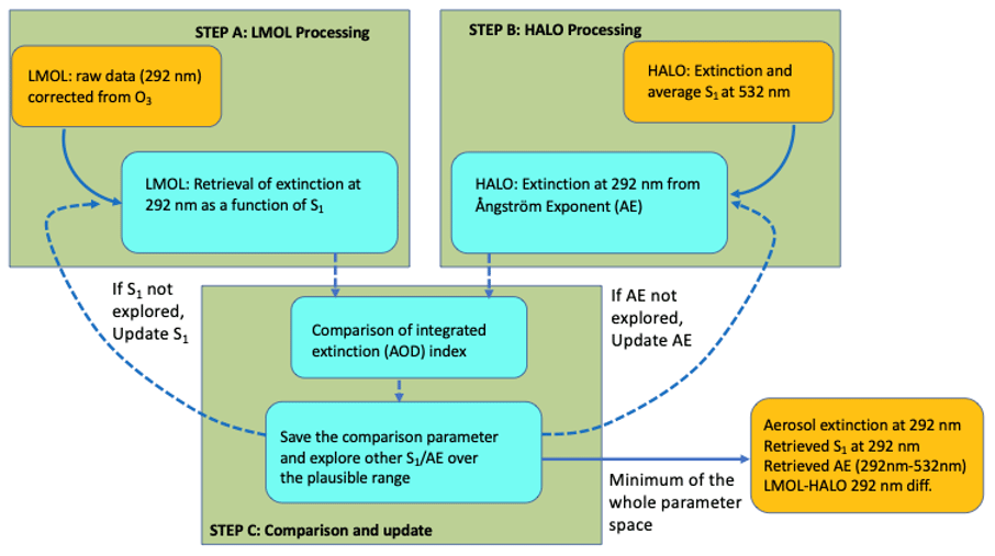
Figure 1Flow chart of the approach used in this work. The cyan section corresponds to the processing needed for the retrieval of the optimal (S1, AE) selection.
2.1 The LMOL system
LMOL is a mobile ground-based O3 differential absorption lidar (DIAL) system that has a transmitter with a 1 kHz diode-pumped Q-switched Nd:YLF 527 nm laser to pump a custom-built Ce:LiCAF tunable UV laser to generate “on” and “off” DIAL wavelengths at 286 and 292 nm. A 40 cm diameter telescope was used to collect the backscatter signal for the far field, and a smaller-diameter wide-field off-axis parabolic mirror was used for the near-field return (De Young et al., 2017; Farris et al., 2019). Both far-field and near-field receiver channels employ analog and photon detection modes using a high-speed Licel data acquisition system to maximize the measurement dynamic range. The current configuration of LMOL can retrieve O3 profiles in the 0.1 to 10 km range at night, with 5 to 10 min temporal averaging (Gronoff et al. 2019, 2021, Farris et al., 2019). During daytime, the maximum altitude reached is typically close to 5 km due to solar background light limitations. LMOL is part of the Tropospheric Ozone Lidar Network (TOLNet), a network of O3 lidars that help evaluate air quality models and complement current and planned satellite retrievals for satellite such as the Tropospheric Emissions: Monitoring of Pollution (TEMPO) mission (Zoogman et al., 2017). LMOL generates data products following the TOLNet protocol for the acquisition, processing, and archiving of the data, thereby assuring the quality and consistency of the data products (Leblanc et al., 2016a, 2016b, 2018). For LMOL data products, the vertical resolution (110 to 990 m) of the O3 profiles varies with altitude to preserve a retrieval uncertainty of within ±10 %, the uncertainty of which is calculated using Poisson statistics of the backscattered photons. LMOL has been used in several campaigns, such as the Ozone Water–Land Environmental Transition Study (OWLETS) I and II, LISTOS (Berkoff et al., 2019; Sullivan et al., 2019; Dacic et al., 2020), the Fire Influence on Regional to Global Environments and Air Quality (FIREX-AQ) joint venture, and the Southern California Ozone Observation Project (SCOOP) (Leblanc et al., 2018). In the context of LISTOS (Wu et al., 2021), and more specifically for the present study, LMOL was deployed at Sherwood Island Park, Westport, CT (41.1182∘ N, 73.3368∘ W; 2.5 m a.s.l.), and obtained measurements between 12 July and 29 August 2018. To obtain the aerosol products, we used the LMOL raw data at 292 nm and the LMOL O3 data.
2.2 The ceilometer located nearby LMOL
A ceilometer (Vaisala CL51) was installed at the Westport site co-located with LMOL (41.1173∘ N, 73.3369∘ W; 3 m a.s.l.) during the LISTOS campaign. A ceilometer is a single-wavelength backscatter lidar system used to monitor cloud base height and aerosol structures (Wang et al., 2018). A semiconductor laser (InGaAs diode laser) with a 3.0 µJ pulse energy and a repetition rate of 6.5 kHz retrieves the atmospheric backscatter at 910 nm to infer the vertical distribution of clouds and aerosols up to 15 km (Lee et al., 2018; Jin et al., 2015). The measured backscatter signal was integrated over 5 s. It is an autonomous eye-safe system that makes 24/7 observations. Although the molecular signal returns are weak because of the low-energy laser and the near-infrared wavelength, the stronger returns from aerosols and clouds can be detected. The CL51 signal is impacted by dark-current noise and daytime solar background, but it is still sufficient to measure signals from boundary layer aerosols up to 3 km (Jin et al., 2015). As a result, the ceilometer can provide the boundary layer evolution and aerosol retrievals up to 3 km for qualitative comparison with the LMOL.
2.3 The HALO aerosol measurement
The NASA airborne High Altitude Lidar Observatory (HALO) is a combined high-spectral-resolution lidar (HSRL) and H2O- and CH4-differential absorption lidar (DIAL) (Nehrir et al., 2017; Wu et al., 2021). HALO employs 1 KHz Nd:YAG pumped optical parametric oscillators to generate the DIAL wavelength for the H2O and CH4 observations. The residual energy from the conversion process is employed for the HSRL technique. HALO employs the HSRL technique at 532 nm, the backscatter technique at 1064nm, and measures depolarization at both 532 and 1064 nm. An I2 vapor cell is used in the receiver to separate the molecular scattering from the total scattering (Hair et al., 2008). This allows for discrimination of aerosol scattering from molecular scattering as well as the independent retrieval of the aerosol extinction and backscatter coefficient (Burton et al., 2013, 2014, 2015; Hair et al., 2008). The lidar extinction-to-backscatter ratio is then available from the HALO-determined aerosol extinction and backscatter coefficients. HALO data are sampled at 0.5 s temporal and 1.25 m vertical resolution. This vertical resolution for the aerosol measurement is increased to 15 m in post-processing to increase the signal-to-noise (SNR) ratio of the intensive and extensive aerosol retrievals. Aerosol backscatter and depolarization products are averaged over 10 s horizontally, and aerosol extinction products are averaged over 60 s horizontally and 150 m vertically. The polarization and HSRL gain ratios are calculated as described in Hair et al. (2008). Operational retrievals also provide the mixing ratio of nonspherical-to-spherical backscatter (Sugimoto and Lee, 2006), the aerosol type (Burton et al., 2012), and the aerosol mixed layer height (Scarino et al., 2014). In this study, the HALO aerosol extinction data are selected when the instrument's flight measurements overpass the LMOL site.
2.4 The CCNY aerosol lidar
The CCNY lidar transmits at 1064, 532, and 355 nm with a flash lamp-pumped Nd:YAG laser with a pulse repetition rate of 30 Hz. A telescope with a 50 cm diameter collects three-wavelength elastic scatter and two Raman-scattering returns (by nitrogen and water vapor excited by a 355 nm laser). The aerosol extinction and backscatter profiles in the troposphere were retrieved, and the AE was derived to distinguish fine-mode aerosol from coarse-mode aerosol. The CCNY lidar return signal detection starts from 0.5 km with a 1 min time average and a 3.75 m vertical data-bin resolution. The planetary boundary layer (PBL) height was estimated from the 1064 nm elastic return because the backscatter signal at this wavelength is more sensitive to aerosol structures than at shorter wavelengths (Wu et al., 2019, 2018, 2021). The CCNY lidar was located in New York City (NYC; 40.8198∘ N, −73.9483∘ W) for remote sensing of the aerosol layer aloft during the LISTOS campaign.
It is important to determine the S1 for the LMOL 292 nm aerosol retrieval. The O3-corrected LMOL attenuated backscatter profile does not contain the information needed to estimate S1. Fortunately, the HALO observations provide the 532 nm extinction and S1 which could help us to learn some information about the aerosol optical properties for cases where the two instruments have coincident observations.
To retrieve the S1, an iterative method with three main steps was used, as shown in Fig. 1. The first step is the retrieval of the aerosol extinction at 292 nm from LMOL. For that, the LMOL raw data are corrected for the O3 absorption. The Fernald method is then used with an empirical S1 (which is modified in subsequent iterations to explore the parameter space). For the current study, the impact of the aerosols was low enough that an iterative correction to the O3 density was not necessary to retrieve the aerosol extinction accurately; for dense aerosols layers, the method described in Browell et al. (1985) would have been used. The second step is the retrieval of the aerosol extinction at 292 nm from HALO. The conversion of the extinction from 532 to 292 nm is done using an assumed AE (between 292 and 532 nm) which is also modified in subsequent iterations to explore the (S1, AE) parameter space. The third step is the comparison of the aerosol extinction from both instruments at 292 nm. The integration of the difference provides the partial aerosol optical depth (AOD) difference, referred to later as the partial AOD index. Once the plausible (S1, AE) parameter space has been explored, there will be a minimum to the partial AOD index which points to the best (S1, AE) for the observed conditions. The LMOL aerosol extinction profile related to optimized S1 and the difference between the LMOL and HALO 292 nm aerosol profile related to the optimized S1, and AE were also recorded for further analysis.
3.1 Method to retrieve aerosol extinction coefficient
LMOL uses the 287 and 292 nm wavelengths for O3 DIAL measurements. The 292 nm “off” wavelength was selected for the aerosol retrieval in this work because O3 has a smaller absorption cross section at this wavelength. The attenuated lidar signal measured by the LMOL system can be represented as follows:
where Pλ(R) is the lidar return signal power; λ is the laser wavelength; Cλ is the lidar system constant; βλ,a(R) is the aerosol volume backscatter coefficient; βλ,m(R) is the molecular volume backscatter coefficient; αλ,a(R) is the aerosol optical extinction coefficient; αλ,m(R) is the molecular optical extinction coefficient (without the O3 extinction); is the O3 absorption cross section; is the O3 number density; and Pλ,0 is the offset, which is contributed by the sky background signal, the amplifier and digitizer offset, and the detector dark current (Fernald, 1984; Young et al., 2009). We also have , where σm is the atmospheric extinction cross section, and Nm is the atmospheric molecular number density. The molecular extinction coefficient and backscatter coefficient are usually calculated from a balloon measurement close to the lidar site or from a model like GEOS-5 (Sasano and Nakane, 1984).
The aerosol extinction-to-backscatter ratio (also known as the lidar ratio) is , and the molecular extinction-to-backscatter ratio is (Kovalev and Eichinger, 2004). The S1 value is dependent on the particle size, shape, and refractive index, and it usually varies from ∼10 to 100 sr (Sasano and Nakane, 1984). We have assumed a constant S1 with range for the aerosol extinction retrieval (Fernald, 1972, 1984). The received LMOL lidar signal at 292 nm could be corrected with the O3 profile to get the elastic lidar attenuated backscatter signal attributed to aerosol and molecular terms as shown in Eq. (2). The O3-corrected range-corrected lidar signal with background subtraction is shown as follows:
We can rearrange Eq. (2) to get the aerosol attenuated backscatter signal X(R):
where
Using Eq. (3) and the aerosol and molecular extinction-to-backscatter ratio, the aerosol extinction coefficient at ranges between the lidar and calibration range Rc is shown in Eq. (4) (Fernald, 1984; Sasano et al., 1985). For convenience, the equations in the following do not include λ.
In order to calculate the aerosol extinction coefficient αa(R), we need to assume S1 and the reference value of the aerosol extinction coefficient at a calibration range Rc. The reference value αa(Rc) must be known or estimated. The calibration range and the reference value could be estimated using the secant method mentioned by Li et al. (2018). We need to pay attention to the fact that all data used in the aerosol retrieval process should have the same vertical resolution. The retrieval is applied to cloud-free profiles after applying cloud screening to the data. This was done using the convolution of the O3-corrected attenuated backscatter signal and a Haar wavelet function to identify cloud edges and then further screening the data using a threshold to separate cloud features (Burton et al., 2010; Compton et al., 2013; Scarino et al., 2014). The aerosol extinction was retrieved for both LMOL far-field photon-counting and far-field analog signal channels. The near-field aerosol retrieval will be described in a separate study. The aerosol extinction profiles for those two channels were merged to a single profile with an overlapping altitude zone from 1.5 to 2 km. The lowest altitude for the retrieved profile is about 0.5 km, and the highest altitude for the retrieved aerosol profile is constrained by the highest altitude of reliable O3 data.
3.2 Selection of the UVB S1 for retrieval
As mentioned in Sect. 1, we focus on case studies from August 2018, especially during the afternoon period on 28 August 2018. The average S1 for HALO S1 profiles at 532 nm was calculated for afternoon data from 28 August 2018. The HALO S1 data mentioned hereafter are the vertically averaged S1 derived from the HALO S1 profile. The frequency distribution of the HALO S1 profiles for the afternoon of 28 August 2018 is shown in Fig. 2a. The mean HALO S1 for 532 nm is ∼55 sr with a 1 s standard deviation of ∼3 sr. As Fig. 2b shows, the mean HALO S1 for all available August measurement is ∼55 with a 1 s standard deviation of ∼6 sr. The HALO 532 nm S1 data were screened using following criteria when calculating the average for each S1 profile: an S1 value larger than 10 sr and less than 100 sr.
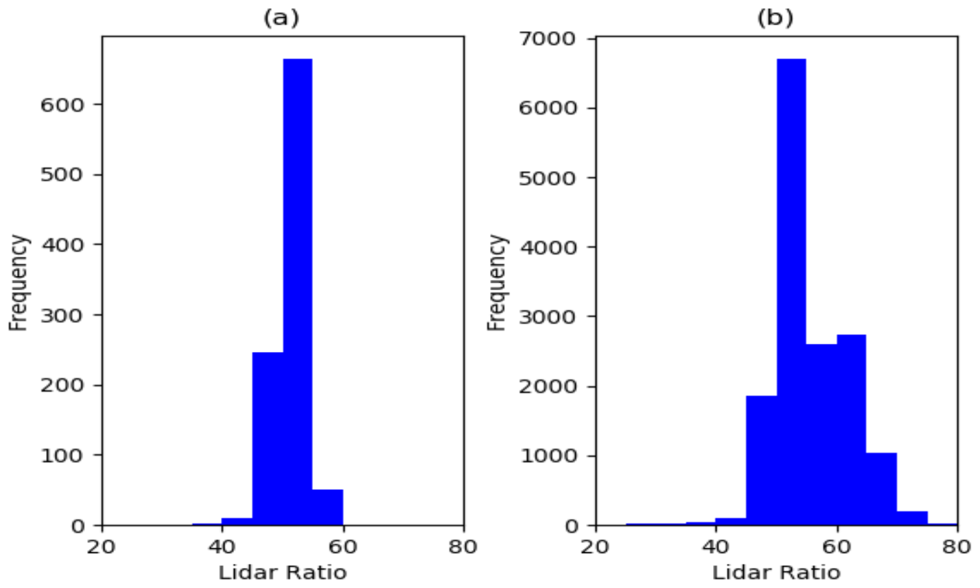
Figure 2(a) A histogram of the average HALO S1 frequency distribution for the afternoon of 28 August, and (b) a histogram of the 5, 6, 15, 16, 24, 28, and 29 August 2018 measurements during the LISTOS campaign.
The following paragraph will introduce the method to identify the S1 at 292 nm and the extinction AE between 292 and 532 nm by calculating the partial AOD difference between the retrieved LMOL 292 nm aerosol extinction profile and the HALO aerosol extinction profile. The AE represents the wavelength dependency of the AOD or extinction coefficient for aerosol. The AE (noted as between two wavelengths, λ1 and λ2, is expressed as shown in the following equation (Wagner and Silva, 2008):
where τ1 and τ2 are the AOD at wavelength λ1 and λ2, respectively. The ideal S1 at 292 nm and the AE between 292 and 532 nm were determined from the retrieved LMOL aerosol extinction profiles and the aerosol profiles provided by co-located HALO measurements using a partial AOD difference method. Figure 3 shows the flow chart for five steps of this partial AOD difference method. In Step 1, the LMOL aerosol extinction, denoted using , was retrieved by incrementing S1(i) from 10 to 90 sr in steps of 5 sr. In Step 2, the LMOL aerosol extinction, , was multiplied by ΔR (7 m in this work) to get the LMOL partial AOD at altitude R, denoted using PAOD. In Step 3, HALO 532 nm aerosol extinction was converted to aerosol extinction at 292 nm with AE (j) and varied from 0.5 to 2.5 in steps of 0.1. The 292 nm HALO aerosol extinction, αHALO, AE(j)(R), was then multiplied by ΔR to obtain the HALO partial AOD at altitude R, denoted using PAODHALO, AE(j)(R). In Step 4, the relative difference of partial AOD (denoted using ΔPAODi,j(R)) between PAOD and PAODHALO, AE(j)(R) was calculated using Eq. (6). In Step 5, the ΔPAODi,j(R)) values were integrated to get the partial AOD difference index, PAODI(i,j), using Eq. (7). In Eq. (7), Rb and Rt are the respective bottom and top altitudes for calculating the PAODI(i,j).

Figure 3Flow chart of the process of calculating the 292 nm S1 and the AE between 532 and 292 nm. i is the integer increment from 2 to 18 that was used to calculate S1 in order to make S1 vary from 10 to 90. j is the integer increment from 5 to 25 that was used to calculate the AE in order to make the AE vary from 0.5 to 2.5. i and j could also be the index of the calculated partial AOD.
The S1(i), AE(j), PAODI(i,j), corresponding LMOL 292 nm aerosol extinction profile, and corresponding LMOL–HALO aerosol profile difference were all recorded. We use the S1(i), AE(j), and PAODI(i,j) data to find the minimum PAODI(i,j) as well as the corresponding S1 and AE, with the latter two terms denoted using S1(ic) and AE(jc), respectively. The LMOL 292 nm aerosol extinction profile corresponding to S1(ic) is the value for the LMOL aerosol retrieval. The LMOL–HALO aerosol profile difference corresponding to S1(ic) and AE(jc) indicates the LMOL aerosol and HALO aerosol extinction comparison. This partial AOD difference method provides details on how to calculate the optimized S1, AE, and it corresponds to the cyan section in Fig. 1.
In order to show how the PAODI changed with the 292 nm S1 and the AE (292 and 532 nm), we further calculated the percentage relative difference of the PAODI compared with PAODImin. An example of this partial AOD difference method at 13:17 EDT on 28 August 2018 is shown in Fig. 4. The PAODI was calculated for altitude regions from 0.5 to 3 km. The results in Fig. 4a show that the selected S1 is 35 sr and the selected AE (292 and 532 nm) is 1.4. Therefore, an S1 of 35 sr is the ideal choice for aerosol extinction retrieval on the afternoon of 28 August 2018. As show in Fig. 4b, the LMOL S1 and the AE (292 and 532 nm) at (40, 1.5) and (30, 1.3) also have a PAODI value very close to PAODImin and could be a potential choice for the LMOL retrieval and comparison. Significant errors can arise when an improper S1 is used for any UV aerosol retrieval that requires an inversion. For example, the value of PAODI using S1=60 and AE =1.4 is about 200 % of the PAODI value using S1=35 and AE =1.4. Thus, the further that S1 deviates from the correct value, the larger the error caused for the UVB aerosol retrieval.
Using the abovementioned process, the selected 292 nm S1 and AE (292 and 532 nm) were derived from all available co-located HALO and LMOL measurements for 5, 6, 16, 24, 28, and 29 August. The results and the HALO average S1 at 532 nm are shown in Table 1. The altitude range for calculating the 292 nm S1 and AE (292 and 532 nm) was from 0.5 to 3 km with the exception of the afternoon flight on 6 August, the morning flight on 16 August, and the afternoon flight on 29 August. In these cases, the altitude range from 0.5 to 2.5 km was used to avoid cloud interference that prevented proper retrieval; these instances are marked using an asterisk in Table 1.
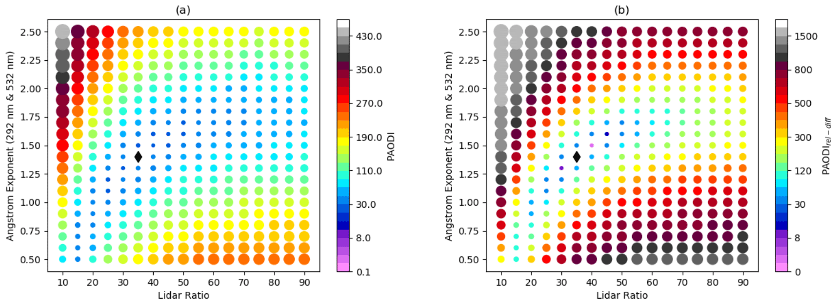
Figure 4(a) The distribution of PAODI according to the 292 nm S1 and AE (292 and 532 nm). The marker color and size show the value of PAODI. The PAODImin was found, and the corresponding S1 and AE (292 and 532 nm) are noted as a black diamond. (b) The distribution of PAODIrel−diff. The marker size and color show the value of PAODIrel−diff. Black diamond shows the minimum value of PAODI and indicates the ideal S1 used for optimized 292 nm aerosol retrieval.
Figure 5 shows the S1 and AE for 292 and 532 nm providing a view of the relationships. As shown in Fig. 5a and b, 532 nm S1 varied between 40 and 70 sr, 292 nm S1 varied between 20 and 55 sr, and the AE (292 and 532 nm) varied from 1 to 1.7. Figure 5a also shows that the 532 nm S1 values are anticorrelated with the AE (532 and 292 nm), with a correlation coefficient of −0.72 and an R2 value of 0.516. The anticorrelation indicates that the S1 values are dependent on the particle size (Giannakaki et al., 2010). The 292 nm S1 does not have a clear correlation with AE (532 and 292 nm), which is probably caused by the different aerosol absorption characteristic at 292 nm. Figure 5c shows that 292 nm S1 values are smaller than 532 nm S1 values for all cases listed in Table 1. The smaller S1 values at UV wavelengths compared with those in the visible at 532 nm show the characteristic feature of aged smoke particles (Wandinger et al., 2002; Haarig et al., 2018, Müller et al., 2005, 2007; Ortiz-Amezcua, 2017). This confirms the previous reports that the air parcel arriving in the northeastern US had passed over active fires in the southeastern US, the northwestern US, or the British Columbian region (Wu et al., 2021; Rogers et al., 2020; Hung et al., 2020).
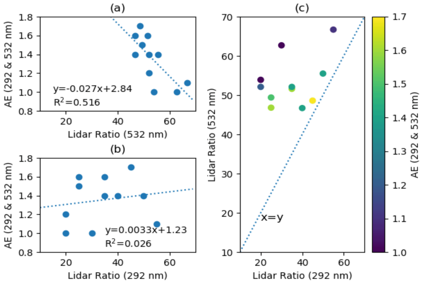
Figure 5The S1 values for 292 and 532 nm as well as the AE (292 and 532 nm) according to Table 1: (a) 532 nm S1 and AE (292 and 532 nm) and (b) 292 nm S1 and AE (292 and 532). (c) Scatterplot of the S1 values for 532 and 292 nm with the color bar showing the AE (292 and 532 nm).
Table 1The LMOL S1 at 292 nm (S1,292), HALO S1 at 532 nm (S1,532), and HALO AE (292 and 532 nm) for August 2018. AM denotes morning, and PM denotes afternoon/evening.
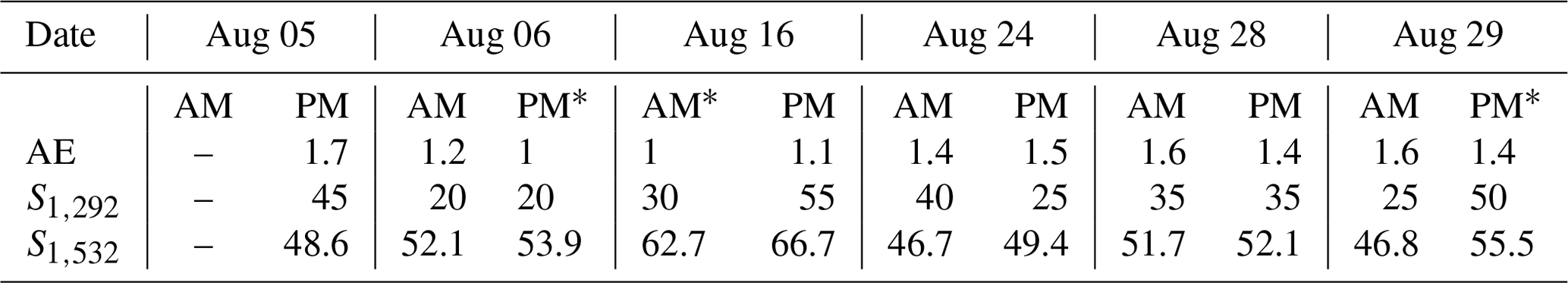
∗ The altitude range from 0.5 to 2.5 km was used to avoid cloud interference that prevented proper retrieval.
4.1 Comparison of the retrieved LMOL result and the HALO aerosol extinction profile
The optimized 292 nm S1 and AE (292 and 532 nm) selected in Table 1 have a corresponding LMOL 292 nm aerosol extinction and a 292 nm HALO aerosol profile comparison. The result of the LMOL–HALO comparison is shown in Fig. 6a–c for the afternoon of 28 August 2018. In Fig. 6a, the LMOL 292 nm aerosol extinction profile is shown in purple and the HALO aerosol extinction profile is shown in blue. As shown in Fig. 6c, the percentage difference is typically less than 10 % between 0.5 and 3 km. The gray shaded region in Fig. 6c shows the ±10 % region. The percentage difference is larger at higher altitudes because the aerosol concentration is lower above the boundary layer. The percentage difference for all available HALO and LMOL aerosol data between 0.5 and 2.5 km was used to calculate the probability distribution function of the percentage difference for 5 % binning. The results in Fig. 6d show that the distribution of the frequency is centered about zero and exhibits a Gaussian distribution. The total number of points used for the comparison is 3146. The height of the peak of the distribution function is 0.175 (as it is normalized to 1). The median error percentage is 1.5 % with a standard deviation of 11 %. These results show that LMOL has the capability to retrieve aerosol extinction at 292 nm with reasonable accuracy. This result also provides the aerosol extinction value in the UVB wavelength range, which helps to understand the UV aerosol optical properties of transported wildfire smoke aerosol. This intercomparison is important because it illustrates the ability of the LMOL aerosol retrieval to capture a consistent aerosol feature when compared to HALO and, thus, produce relevant data for campaign analysis of the relationship between aerosols and O3 features.
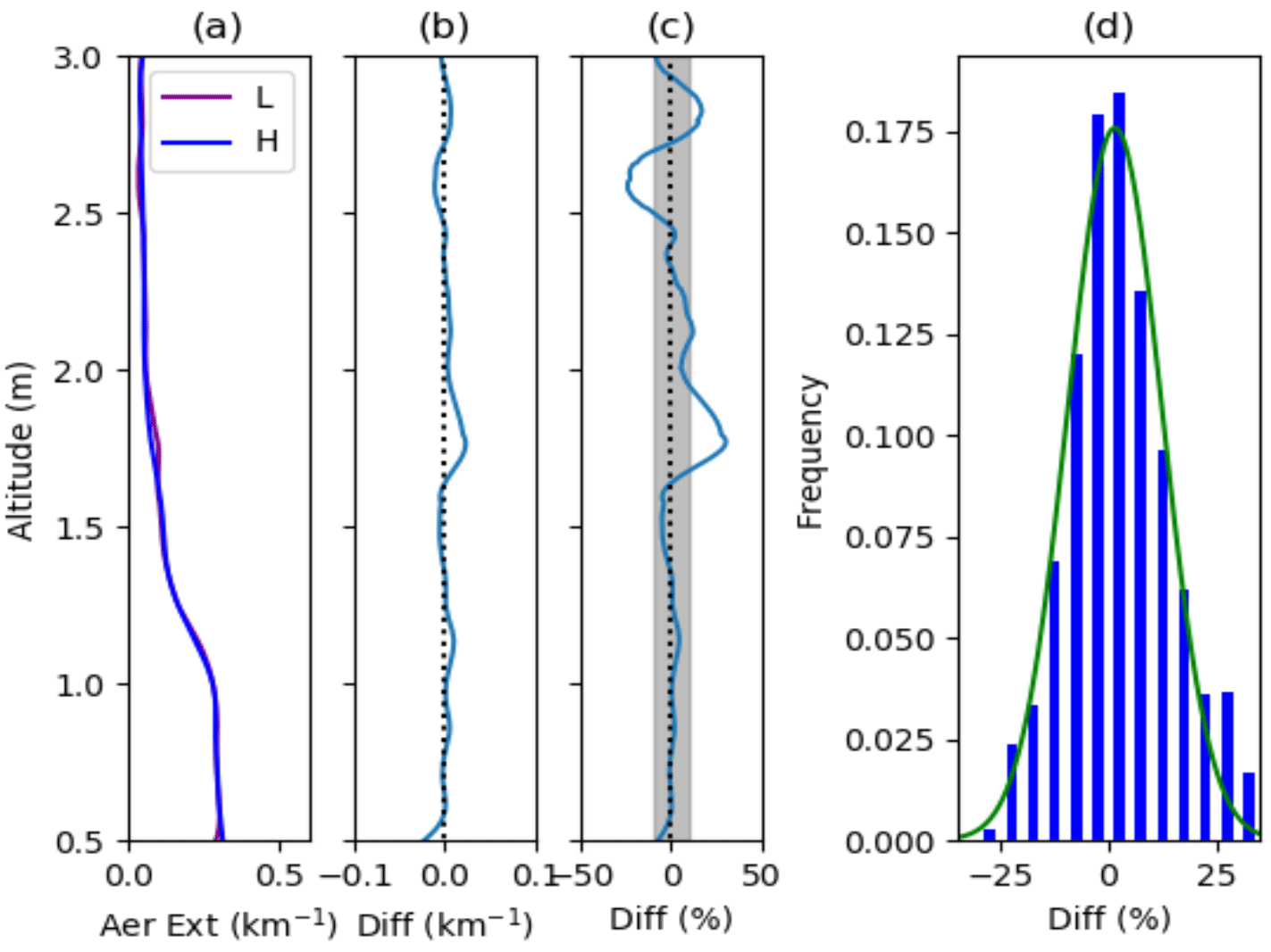
Figure 6Comparison of the LMOL- and HALO-derived 292 nm aerosol extinction coefficient at 13:17 EDT on the afternoon of 28 August 2018 using the S1 and AE values selected in Sect. 3.2. The HALO aerosol extinction profile is converted from the 532 nm aerosol extinction product. Panel (a) shows the LMOL and HALO aerosol extinction; panel (b) displays the difference between the LMOL and HALO aerosol extinction; panel (c) gives the percentage difference between the LMOL and HALO aerosol extinction; and panel (d) shows the error (percentage difference) probability distribution function for all available comparisons between 0.5 and 2.5 km for August 2018. In panel (d), the width between each bar shows 5 % difference.
4.2 Comparisons between LMOL, the CCNY lidar, and CL51
To examine the LMOL retrieval beyond just the HALO overpass times, Fig. 7 provides a curtain plot of the 28 August LMOL 292 nm aerosol extinction compared with a co-located ceilometer CL51 910 nm backscatter signal and with the CCNY lidar (located in NYC) aerosol extinction (converted from 532 to 292 nm using an AE of 1.4). This allowed us observe boundary layer development and examine the aerosol variation features during the course of the day. The PBL height increases after 10:00 EDT and reaches a maximum at 17:00 EDT. The comparison between the CCNY aerosol extinction and the LMOL aerosol extinction shows that the retrieved LMOL UV aerosol extinction is qualitatively consistent. The difference in the aerosol extinction between the LMOL and CCNY measurements is probably caused by atmospheric variation among different locations over a distance of about 60 km. The PBL height was retrieved by applying a wavelet method to the LMOL and CCNY aerosol data (Brooks et al., 2003; Compton et al., 2013; Scarino et al., 2014). The PBL height of the ceilometer was obtained from the CL51 data product, which could be obtained from the LISTOS archive data. The PBL height is overlaid on the aerosol and O3 curtain plot in Fig. 7a–d. LMOL-retrieved UVB aerosol extinction and the co-located CL51 aerosol backscatter show exactly the same variation for the PBL evolution except for the higher backscatter between 12:00 and 14:00 EDT. This is due to the fact that cloud screening was applied to the LMOL UVB aerosol retrieval process. This intercomparison is important because it illustrates the ability of the LMOL aerosol retrieval to capture a consistent aerosol feature when compared to other lidar systems and, thus, to produce relevant data for campaign analysis of the relationship between aerosols and O3 features. Capturing aerosol extinction between 0.5 and 3.0 km is very useful because it will help us to retrieve the PBL height and to learn more about aerosol properties in the lower part of troposphere. Furthermore, aerosol profiling information can still play an important role in model intercomparisons and satellite retrievals.
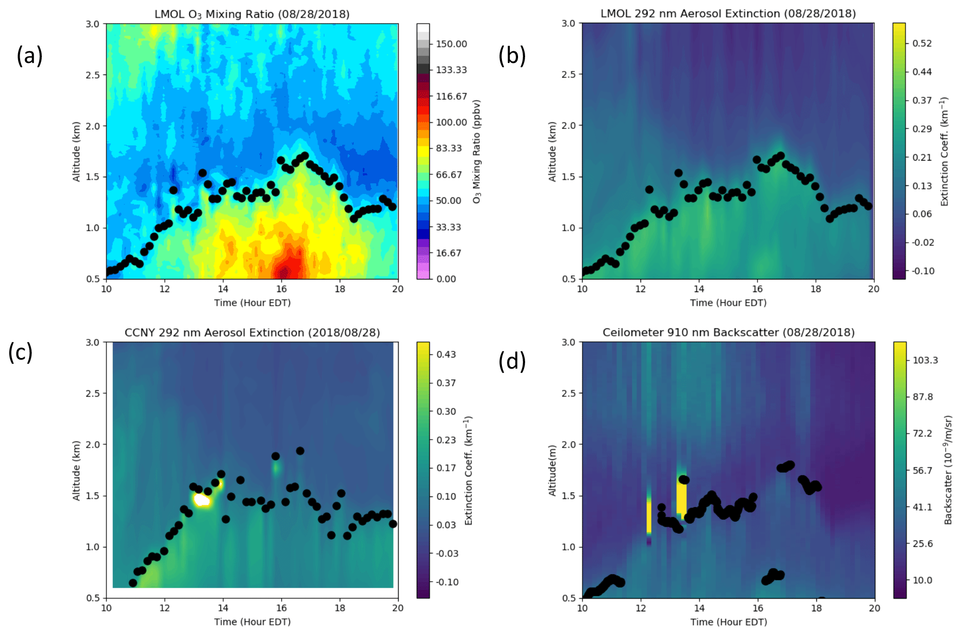
Figure 7(a) The O3 variation, (b) the retrieved LMOL UVB aerosol extinction coefficient curtain plot, (c) the CCNY lidar aerosol extinction coefficient (converted to 292 nm), and (d) the 910 nm ceilometer CL51 (same location as LMOL) backscatter for 28 August 2018. The black dot on the curtain plots in panels (b)–(d) shows the PBL height.
In this section, the sensitivity of the algorithm to uncertainty in the input parameters is analyzed for the 28 August 2018 case. The aerosol extinction retrieval uncertainties caused by the lidar detection noise, reference value estimation, atmospheric molecular density, O3 concentration uncertainty, and the S1 will be discussed. The quantitative estimation of the aerosol extinction and backscatter uncertainty is challenging, and no standardized recommendation exists (Leblanc et al., 2016b). In this work, the total uncertainty of the retrieved extinction coefficient is calculated by following standard propagation of error practices. The retrieved aerosol profile depends on several instrumental and physical parameters for the lidar system. The measurement model for the system is presented as Eq. (9). The individual values y of the quantity Y are shown in Eq. (10) (Leblanc et al., 2016b).
The combined standard uncertainty (uy) is obtained using the individual standard measurement uncertainties associated with the input quantities in Eq. (9). As shown in Eq. (11), uy equals the positive squared root of the combined variance for all variables that are independent (Leblanc et al., 2016b):
As shown in Sect. 2, the signal was used to calculate the aerosol extinction noted as X(R) and shown as Eq. (12):
The detection noise uncertainty is derived from Poisson statistics associated with the probability of the detection of a repeated random event. Following Leblanc et al. (2016b), the subscript “DET” was used for detection noise. The uncertainty in the raw signal P(R) caused by detection noise could be expressed as shown in Eq. (13) and reflects purely random effects during detection (Russell et al., 1979).
It is propagated to the background- and O3-corrected signal X(R) by apply Eq. (11) to Eq. (12):
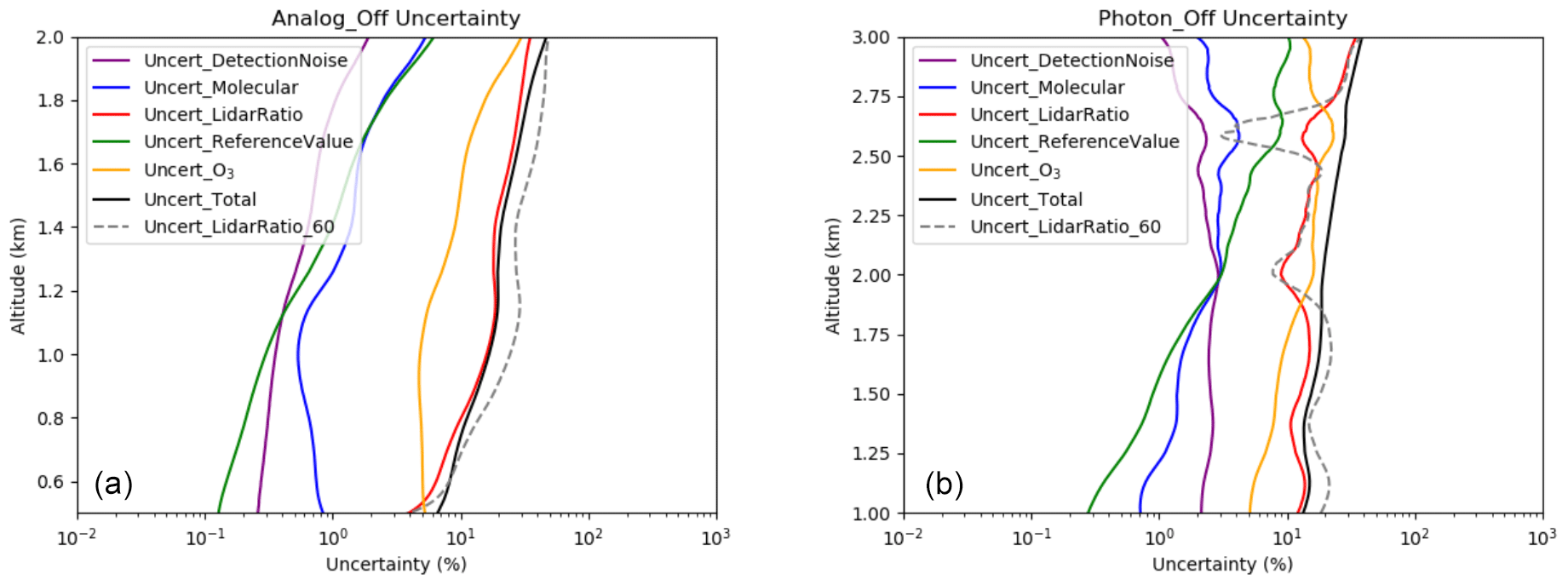
Figure 8The uncertainty budget for the LMOL (a) analog channel and (b) photon channel for the 28 August 2018 afternoon retrieval. The uncertainties are attributed to different factors: detection noise (purple), molecular number density (blue), S1 (red), reference value (green), uncertainty of O3 (orange), and total uncertainty (black). The uncertainty caused by using 60 sr as the S1 is shown using a dashed gray line.
Similarly, the O3 uncertainty is noted as , and it is propagated to the background- and O3-corrected signal X(R) as show in Eq. (15):
The propagated uncertainty caused by detection noise and O3 could be established by apply Eq. (11) to Eq. (4) as follows:
Thus, the total uncertainty can be established as shown in Eq. (18).
The uncertainty shown in Eq. (18) considers the impact of integral uncertainty from the targeted altitude to the reference point, as Eq. (4) includes the integral accounting for the molecular extinction and the O3-corrected return lidar signal of the target altitude to the reference point. is the atmospheric molecular number density uncertainty, which we set as 1 % following the result from Kuang et al. (2020). The S1 is assigned 35±15 sr for this example, and the uncertainty of the is about ±40 %. The uncertainty of the reference value is taken as 10 times for the total uncertainty analysis, as show in Eq. (18).
We calculated the uncertainties of the analog channel and the photon channel separately, so we could assess how the different parameters impacted the retrieval uncertainty for both channels. The photocurrent for the photomultiplier tube (PMT) analog mode no longer follows a strict Poisson distribution, but there still may be a quantitative estimate of this uncertainty. The uncertainty of the detection noise for the PMT analog channel is recalculated using the method mentioned in Liu et al. (2006), and the results are shown in Fig. 8a. As Fig. 8 shows, the uncertainty caused by the detection noise is small for both channels. The uncertainty caused by the reference value and the molecular number density is less than 10 % for both channels. Ozone uncertainty is 10 % for the LMOL system and generally causes less than 20 % aerosol extinction uncertainty for the analog channel and photon channel. The uncertainty of the S1 causes about 4 %–30 % uncertainty for both the analog and photon channels. The uncertainty of the S1 and O3 dominate the total uncertainty for both channels. We also show the uncertainty caused by using 60 sr as S1 for UVB aerosol retrieval for the afternoon of 28 August 2018. It was found that an S1 of 60 would increase the aerosol retrieval uncertainty in the PBL but that the uncertainty did not change much above 2 km except in a layer located at 2.6 km.
For the first time, the aerosol extinction coefficient profiles, retrieved from the LMOL 292 nm attenuated backscatter using the Fernald algorithm, are compared with airborne HALO data. A partial AOD difference method was introduced to determine the optimized value for 292 nm S1 and AE (292 and 532 nm) from these instruments. The optimized S1 and AE (292 and 532 nm) improved the accuracy of the UVB aerosol retrieval. In addition, knowledge of these parameters can improve our understanding of the aerosol properties; for example, the case studies in the present paper demonstrated that we were in the presence of transported smoke. The intercomparison between HALO and LMOL aerosol products showed an agreement within 10 % up to 3 km after the optimization method was applied in the case of the 28 August 2018. The retrieved LMOL 292 nm aerosol was also compared with co-located ceilometer and CCNY aerosol lidar. This showed that LMOL could capture a consistent aerosol feature and mixing layer evolution. Error analysis showed that the uncertainty from O3 and S1 dominates the 292 nm aerosol retrieval and needs to be carefully considered in the retrievals of aerosol profiles of all of the TOLNet lidars. In cases for which there are no HALO data, a priori determinations from differing aerosol types based on this kind of analysis work will serve to provide reasonable S1 values. Consequently, further research is needed to characterize S1 and AE at UVB wavelengths: first, an effort should be made to determine the variation in S1 and AE with altitude by carefully addressing the uncertainties in the HALO S1 profile products; second, additional co-located LMOL–HSRL measurements should be done to evaluate S1 and AE for different aerosol types (smoke, dust, marine aerosol, and pollutant aerosol). This characterization could ultimately enable the use of equipment with a better availability than HSRL instruments (e.g., micropulse lidars) in order to provide the ancillary data necessary for the aerosol extinction retrieval.
The LMOL O3 raw data used in this study are available upon request from Timothy A. Berkoff and Guillaume Gronoff. LMOL O3 data from the Long Island Sound Tropospheric Ozone Study (LISTOS) campaign are available through the NASA Atmospheric Science Data Center (ASDC) at https://doi.org/10.5067/SUBORBITAL/LISTOS/DATA001 (NASA/LARC/SD/ASDC, 2020). The HALO aerosol data from the Long Island Sound Tropospheric Ozone Study (LISTOS) campaign are available through the NASA Atmospheric Science Data Center (ASDC) at https://doi.org/10.5067/SUBORBITAL/LISTOS/DATA001 (NASA/LARC/SD/ASDC, 2020).
The supplement related to this article is available online at: https://doi.org/10.5194/amt-15-2465-2022-supplement.
LL and TAB formulated the overarching research goals. GG supported the O3 data analysis, which was a key factor in the aerosol retrieval algorithm, and plotted Fig. 1, outlining the flow chart of the approach used in this work. LL and JS carried out the UV aerosol extinction retrieval calculation. LL undertook the S1 and AE determination as well as the aerosol extinction comparison between LMOL and HALO. ARN provided the HALO aerosol data product and the HALO instrument introduction for the paper. YW and FM contributed CCNY lidar aerosol data and CCNY PBL height data. SK contributed to the UV aerosol retrieval algorithm. LL wrote the initial draft of the paper with contributions from all co-authors. All authors reviewed and agreed upon the final paper.
The contact author has declared that neither they nor their co-authors have any competing interests.
Publisher's note: Copernicus Publications remains neutral with regard to jurisdictional claims in published maps and institutional affiliations.
The authors gratefully acknowledge support from the NASA Postdoctoral Program, which enabled this study. LMOL and HALO lidar participation in the LISTOS campaign was made possible by funding from the NASA Tropospheric Composition Program. We gratefully acknowledge William Carrion and Joseph Sparrow for LMOL operational support and the Connecticut Department of Energy and Environmental Protection for providing site support that enabled LMOL operations at the Westport location. The HALO team acknowledges support from the Langley Research Center Research Services Division for the operation and maintenance of the King Air B200 aircraft for the duration of the LISTOS campaign. The authors are grateful to Susan Kooi and James Collins for their contribution to analysis and archiving of the HALO HSRL data set, James Szykman and Travis Knepp for Westport ceilometer data, and Daniel B. Phoenix for his valuable comments and his help with editing the manuscript. Yonghua Wu and Fred Moshary are supported by the New York State Energy Resources Development Authority (grant no. 137482), NESCAUM (grant nos. 2411 and 2417), and NOAA-CESSRST (under cooperative agreement grant no. NA16SEC4810008).
This research has been supported by the NASA Postdoctoral program, the New York State Energy Resources Development Authority (grant no. 137482), NESCAUM (grant nos. 2411 and 2417), and NOAA-CESSRST (grant no. NA16SEC4810008).
This paper was edited by Omar Torres and reviewed by two anonymous referees.
Aggarwal, M., Whiteway, J., Seabrook, J., Gray, L., Strawbridge, K., Liu, P., O'Brien, J., Li, S.-M., and McLaren, R.: Airborne lidar measurements of aerosol and ozone above the Canadian oil sands region, Atmos. Meas. Tech., 11, 3829–3849, https://doi.org/10.5194/amt-11-3829-2018, 2018.
Andreae, M. O. and Merlet, P.: Emission of trace gases and aerosols from biomass burning, Global Biogeochem. Cy., 15, 955–966, https://doi.org/10.1029/2000GB001382, 2001.
Bais, A. F., Zerefos, C. S., Meleti, C., Ziomas, I. C., and Tourpali, K.: Spectral measurements of solar UVB radiation and its relations to total ozone, SO2, and clouds, J. Geophys. Res.-Atmos., 98, 5199–5204, https://doi.org/10.1029/92jd02904, 1993.
Berkoff, T., Gronoff, G., Sullivan, J., Nino, L., Carrion, W., Twigg, L., Sparrow, J., Knepp, T., Tully, D., Chaffe, M., Babich, P., Valin, L., and Szykman, J.: Ozone Lidar Observations During the Long Island Sound Tropospheric Ozone Study, LISTOS Meeting, Albany, New York, 11 April 2019, https://www.nescaum.org/documents/listos/presentations-from-listos-meeting-albany-ny/berkoff.pdf (last access: 20 April 2022), 2019.
Brooks, I. M.: Finding Boundary Layer Top: Application of a Wavelet Covariance Transform to Lidar Backscatter Profiles, J. Atmos. Ocean. Tech., 20, 1092–1105, https://doi.org/10.1175/1520-0426(2003)020<1092:FBLTAO>2.0.CO;2, 2003.
Browell, E. V., Ismail, S., and Shipley, S. T.: Ultraviolet DIAL measurements of O3 profiles in regions of spatially inhomogeneous aerosols, Appl. Opt., 24, 2827–2836, https://doi.org/10.1364/ao.24.002827, 1985.
Burton, S. P., Ferrare, R. A., Hostetler, C. A., Hair, J. W., Kittaka, C., Vaughan, M. A., Obland, M. D., Rogers, R. R., Cook, A. L., Harper, D. B., and Remer, L. A.: Using Airborne High Spectral Resolution Lidar Data to Evaluate Combined Active Plus Passive Retrievals of Aerosol Extinction Profiles, J. Geophys. Res., 115, D00H15, https://doi.org/10.1029/2009JD012130, 2010.
Burton, S. P., Ferrare, R. A., Hostetler, C. A., Hair, J. W., Rogers, R. R., Obland, M. D., Butler, C. F., Cook, A. L., Harper, D. B., and Froyd, K. D.: Aerosol classification using airborne High Spectral Resolution Lidar measurements – methodology and examples, Atmos. Meas. Tech., 5, 73–98, https://doi.org/10.5194/amt-5-73-2012, 2012.
Burton, S. P., Ferrare, R. A., Vaughan, M. A., Omar, A. H., Rogers, R. R., Hostetler, C. A., and Hair, J. W.: Aerosol classification from airborne HSRL and comparisons with the CALIPSO vertical feature mask, Atmos. Meas. Tech., 6, 1397–1412, https://doi.org/10.5194/amt-6-1397-2013, 2013.
Burton, S. P., Vaughan, M. A., Ferrare, R. A., and Hostetler, C. A.: Separating mixtures of aerosol types in airborne High Spectral Resolution Lidar data, Atmos. Meas. Tech., 7, 419–436, https://doi.org/10.5194/amt-7-419-2014, 2014.
Burton, S. P., Hair, J. W., Kahnert, M., Ferrare, R. A., Hostetler, C. A., Cook, A. L., Harper, D. B., Berkoff, T. A., Seaman, S. T., Collins, J. E., Fenn, M. A., and Rogers, R. R.: Observations of the spectral dependence of linear particle depolarization ratio of aerosols using NASA Langley airborne High Spectral Resolution Lidar, Atmos. Chem. Phys., 15, 13453–13473, https://doi.org/10.5194/acp-15-13453-2015, 2015.
Carlund, T., Kouremeti, N., Kazadzis, S., and Gröbner, J.: Aerosol optical depth determination in the UV using a four-channel precision filter radiometer, Atmos. Meas. Tech., 10, 905–923, https://doi.org/10.5194/amt-10-905-2017, 2017.
Compton, J. C., Delgado, R., Berkoff, T. A., and Hoff, R. M.: Determination of planetary boundary layer height on short spatial and temporal scales: a demonstration of the covariance wavelet transform in ground-based wind profiler and lidar measurements, J. Atmos. Ocean. Tech., 30, 1566–1575, https://doi.org/10.1175/JTECH-D-12-00116.1, 2013.
Cottle, P., Strawbridge, K., and McKendry, I.: Long-range transport of Siberian wildfire smoke to British Columbia: Lidar observations and air quality impacts, Atmos. Environ., 90, 71–77, https://doi.org/10.1016/j.atmosenv.2014.03.005, 2014.
Dacic, N., Sullivan, J. T., Knowland, K. E., Wolfe, G. M., Oman, L. D., Berkoff, T. A., and Gronoff, G. P.: Evaluation of NASA's high-resolution global composition simulations: Understanding a pollution event in the Chesapeake Bay during the summer 2017 OWLETS campaign, Atmos. Environ., 222, 117133, https://doi.org/10.1016/j.atmosenv.2019.117133, 2020.
De Young, R., Carrion, W., Ganoe, R., Pliutau, D., Gronoff, G., Berkoff, T., and Kuang, S.: Langley mobile ozone lidar: ozone and aerosol atmospheric profiling for air quality research, Appl. Opt., 56, 721–730, https://doi.org/10.1364/ao.56.000721, 2017.
Dreessen, J., Sullivan, J., and Delgado, R.: Observations and impacts of transported Canadian wildfire smoke on ozone and aerosol air quality in the Maryland region on June 9–12, 2015, J. Air Waste Manage Assoc., 66, 842–862, https://doi.org/10.1080/10962247.2016.1161674, 2016.
Farris, B. M., Gronoff, G. P., Carrion, W., Knepp, T., Pippin, M., and Berkoff, T. A.: Demonstration of an off-axis parabolic receiver for near-range retrieval of lidar ozone profiles, Atmos. Meas. Tech., 12, 363–370, https://doi.org/10.5194/amt-12-363-2019, 2019.
Fernald, F. G.: Analysis of atmospheric lidar observations: some comments, Appl. Optics, 23, 652–653, https://doi.org/10.1364/AO.23.000652, 1984.
Fernald, F. G., Herman, B. M., and Reagan, J. A.: Determination of aerosol height distributions with lidar, J. Appl. Meteorol., 11, 482–489, https://doi.org/10.1175/1520-0450(1972)011<0482:DOAHDB>2.0.CO;2, 1972.
Giannakaki, E., Balis, D. S., Amiridis, V., and Zerefos, C.: Optical properties of different aerosol types: seven years of combined Raman-elastic backscatter lidar measurements in Thessaloniki, Greece, Atmos. Meas. Tech., 3, 569–578, https://doi.org/10.5194/amt-3-569-2010, 2010.
Gronoff, G., Robinson, J., Berkoff, T., Swap, R., Farris, B., Schroeder, J., Halliday, H. S., Knepp, T., Spinei, E., Carrion, W., and Adcock, E. E.: A method for quantifying near range point source induced O3 titration events using Co-located Lidar and Pandora measurements, Atmos. Environ., 204, 43–52, https://doi.org/10.1016/j.atmosenv.2019.01.052, 2019.
Gronoff, G., Berkoff, T., Knowland, K., E., Lei, L., Shook, M., Fabbri, B., Carrion, W., and Langford, A.: Case study of stratospheric Intrusion above Hampton, Virginia: lidar-observation and modeling analysis, Atmos. Environ., 118498, 1–12, https://doi.org/10.1016/j.atmosenv.2021.118498, 2021.
Haarig, M., Ansmann, A., Baars, H., Jimenez, C., Veselovskii, I., Engelmann, R., and Althausen, D.: Depolarization and lidar ratios at 355, 532, and 1064 nm and microphysical properties of aged tropospheric and stratospheric Canadian wildfire smoke, Atmos. Chem. Phys., 18, 11847–11861, https://doi.org/10.5194/acp-18-11847-2018, 2018.
Hair, J. W., Hostetler, C. A., Cook, A. L., Harper, D. B., Ferrare, R. A., Mack, T. L., Welch, W., Izquierdo, L. R., and Hovis, F. E.: Airborne High Spectral Resolution Lidar for profiling aerosol optical properties, Appl. Optics, 47, 6734–6752, https://doi.org/10.1364/AO.47.006734, 2008.
Hung, W. T., Lu, C. H. S., Shrestha, B., Lin, H. C., Lin, C. A., Grogan, D., and Joseph, E.: The impacts of transported wildfire smoke aerosols on surface air quality in New York State: A case study in summer 2018, Atmos. Environ., 227, 117415, https://doi.org/10.1016/j.atmosenv.2020.117415, 2020.
Jin, Y., Kai, K., Kawai, K., Nagai, T., Sakai, T., Yamazaki, A., Uchiyama, A., Batdorj, D., Sugimoto, N., and Nishizawa, T.: Ceilometer calibration for retrieval of aerosol optical properties, J. Quant. Spectrosc. Ra., 153, 49–56, https://doi.org/10.1016/j.jqsrt.2014.10.009, 2015.
Kovalev, V. A. and Eichinger, W. E.: Elastic Lidar Theory, Practice, and Analysis Methods, 1st edn., John Wiley & Sons Inc., Hoboken, New Jersey, USA, https://doi.org/10.1002/0471643173, 2004.
Kuang, S., Wang, B., Newchurch, M. J., Knupp, K., Tucker, P., Eloranta, E. W., Garcia, J. P., Razenkov, I., Sullivan, J. T., Berkoff, T. A., Gronoff, G., Lei, L., Senff, C. J., Langford, A. O., Leblanc, T., and Natraj, V.: Evaluation of UV aerosol retrievals from an ozone lidar, Atmos. Meas. Tech., 13, 5277–5292, https://doi.org/10.5194/amt-13-5277-2020, 2020.
Leblanc, T., Sica, R. J., van Gijsel, J. A. E., Godin-Beekmann, S., Haefele, A., Trickl, T., Payen, G., and Gabarrot, F.: Proposed standardized definitions for vertical resolution and uncertainty in the NDACC lidar ozone and temperature algorithms – Part 1: Vertical resolution, Atmos. Meas. Tech., 9, 4029–4049, https://doi.org/10.5194/amt-9-4029-2016, 2016a.
Leblanc, T., Sica, R. J., van Gijsel, J. A. E., Godin-Beekmann, S., Haefele, A., Trickl, T., Payen, G., and Liberti, G.: Proposed standardized definitions for vertical resolution and uncertainty in the NDACC lidar ozone and temperature algorithms – Part 2: Ozone DIAL uncertainty budget, Atmos. Meas. Tech., 9, 4051–4078, https://doi.org/10.5194/amt-9-4051-2016, 2016b.
Leblanc, T., Brewer, M. A., Wang, P. S., Granados-Muñoz, M. J., Strawbridge, K. B., Travis, M., Firanski, B., Sullivan, J. T., McGee, T. J., Sumnicht, G. K., Twigg, L. W., Berkoff, T. A., Carrion, W., Gronoff, G., Aknan, A., Chen, G., Alvarez, R. J., Langford, A. O., Senff, C. J., Kirgis, G., Johnson, M. S., Kuang, S., and Newchurch, M. J.: Validation of the TOLNet lidars: the Southern California Ozone Observation Project (SCOOP), Atmos. Meas. Tech., 11, 6137–6162, https://doi.org/10.5194/amt-11-6137-2018, 2018.
Lee, S., Hwang, S. O., Kim, J., and Ahn, M. H.: Characteristics of cloud occurrence using ceilometer measurements and its relationship to precipitation over Seoul, Atmos. Res., 201, 46–57, https://doi.org/10.1016/j.atmosres.2017.10.010, 2018.
Li, H., Chang, J., Xu, F., Liu, B., Liu, Z., Zhu, L., and Yang, Z.: An RBF neural network approach for retrieving atmospheric extinction coefficients based on lidar measurements, Appl. Phys. B, 124, 1–8, https://doi.org/10.1007/s00340-018-7055-1, 2018.
Liu, Z., Hunt, W., Vaughan, M., Hostetler, C., McGill, M., Powell, K.,Winker, D., and Hu, Y.: Estimating random errors due to shot noise in backscatter lidar observations, Appl. Optics, 45, 4437–4447, 2006.
Lopes, F. J. S., Landulfo, E., and Vaughan, M. A.: Evaluating CALIPSO's 532 nm lidar ratio selection algorithm using AERONET sun photometers in Brazil, Atmos. Meas. Tech., 6, 3281–3299, https://doi.org/10.5194/amt-6-3281-2013, 2013.
Moozhipurath, R. K., Kraft, L., and Skiera, B.: Evidence of protective role of Ultraviolet-B (UVB) radiation in reducing COVID-19 deaths, Sci. Rep., 10, 17705, https://doi.org/10.1038/s41598-020-74825-z, 2020.
Müller, D., Mattis, I., Wandinger, U., Ansmann, A., Althausen, D., and Stohl, A.: Raman lidar observations of aged Siberian and Canadian forest fire smoke in the free troposphere over Germany in 2003: microphysical particle characterization, J. Geophys. Res., 110, D17201, https://doi.org/10.1029/2004JD005756, 2005.
Müller, D., Ansmann, A., Mattis, I., Tesche, M., Wandinger, U., Althausen, D., and Pisani, G.: Aerosol-type-dependent lidar ratios observed with Raman lidar, J. Geophys. Res., 112, D16202, https://doi.org/10.1029/2006JD008292, 2007.
NASA/LARC/SD/ASDC: Aeolus CalVal HALO Aerosol and Water Vapor Profiles and Images, NASA Langley Atmospheric Science Data Center DAAC [data set], https://doi.org/10.5067/SUBORBITAL/LISTOS/DATA001, 2020.
Nehrir, A. R., Kiemle, C., Lebsock, M. D., Kirchengast, G., Buehler, S. A., Löhnert, U., Liu, C.-L., Hargrave, P. C., Barrera-Verdejo, M., and Winker, D. M.: Emerging Technologies and Synergies for Airborne and Space-Based Measurements of Water Vapor Profiles, Surv. Geophys., 38, 1445–1482, https://doi.org/10.1007/s10712-017-9448-9, 2017.
Nicolae, D., Nemuc, A., Müller, D., Talianu, C., Vasilescu, J., Belegante, L., and Kolgotin, A.: Characterization of fresh and aged biomass burning events using multiwavelength Raman lidar and mass spectrometry, J. Geophys. Res.-Atmos., 118, 2956–2965, https://doi.org/10.1002/jgrd.50324, 2013.
Omar, A. H., Winker, D. M., Vaughan, M. A., Hu, Y., Trepte, C. R., Ferrare, R. A., Lee, K. P., Hostetler, C. A., Kittaka, C., Rogers, R. R., and Kuehn, R. E.: The CALIPSO Automated Aerosol Classification and Lidar Ratio Selection Algorithm, J. Atmos. Ocean. Tech., 26, 1994–2014, https://doi.org/10.1175/2009JTECHA1231.1, 2009.
Ortiz-Amezcua, P., Guerrero-Rascado, J. L., Granados-MunÞoz, M. J., Benavent-Oltra, J. A., Böckmann, C., Samaras, S., Stach-lewska, I. S., Janicka, L., Baars, H., Bohlmann, S., and Alados-Arboledas, L.: Microphysical characterization of long-range transported biomass burning particles from North America at three EARLINET stations, Atmos. Chem. Phys., 17, 5931–5946, https://doi.org/10.5194/acp-17-5931-2017, 2017.
Phuleria, H. C., Fine, P. M., Zhu, Y. F., and Sioutas, C.: Air quality impacts of the October 2003 Southern California wildfires, J. Geophys. Res., 110, 1–11, https://doi.org/10.1029/2004JD004626, 2005.
Reid, J. S., Koppmann, R., Eck, T. F., and Eleuterio, D. P.: A review of biomass burning emissions part II: intensive physical properties of biomass burning particles, Atmos. Chem. Phys., 5, 799–825, https://doi.org/10.5194/acp-5-799-2005, 2005.
Rogers, H. M., Ditto, J. C., and Gentner, D. R.: Evidence for impacts on surface-level air quality in the northeastern US from long-distance transport of smoke from North American fires during the Long Island Sound Tropospheric Ozone Study (LISTOS) 2018, Atmos. Chem. Phys., 20, 671–682, https://doi.org/10.5194/acp-20-671-2020, 2020.
Russell, P. B., Swissler, T. J., and McCormick, M. P.: Methodology for error analysis and simulation of lidar aerosol measurements, Appl. Optics, 18, 3783–3797, https://doi.org/10.1364/AO.18.003783, 1979.
Sasano, Y. and Nakane, H.: Significance of the extinctionbackscatter ratio and the boundary value term in the solution for the two-component lidar equation, Appl. Opt., 23, 1–13, https://doi.org/10.1364/AO.23.0011_1, 1984.
Sasano, Y., Browell, E. V., and Ismail, S.: Error caused by using a constant extinctionbackscattering ratio in the lidar solution, Appl. Opt., 24, 3929–3932, https://doi.org/10.1364/AO.24.003929, 1985.
Scarino, A. J., Obland, M. D., Fast, J. D., Burton, S. P., Ferrare, R. A., Hostetler, C. A., Berg, L. K., Lefer, B., Haman, C., Hair, J. W., Rogers, R. R., Butler, C., Cook, A. L., and Harper, D. B.: Comparison of mixed layer heights from airborne high spectral resolution lidar, ground-based measurements, and the WRF-Chem model during CalNex and CARES, Atmos. Chem. Phys., 14, 5547–5560, https://doi.org/10.5194/acp-14-5547-2014, 2014.
Schoennagel, T., Balch, J. K., Brenkert-Smith, H., Dennison, P. E., Harvey, B. J., Krawchuk, M. A., Mietkiewicz, N., Morgan, P., Moritz, M. A., Rasker, R., Turner, M. G., and Whitlock, C.: Adapt to more wildfire in western North American forests as climate changes, P. Natl. Acad. Sci. USA, 114, 4582–4590, https://doi.org/10.1073/pnas.1617464114, 2017.
Strawbridge, K. B., Travis, M. S., Firanski, B. J., Brook, J. R., Staebler, R., and Leblanc, T.: A fully autonomous ozone, aerosol and nighttime water vapor lidar: a synergistic approach to profiling the atmosphere in the Canadian oil sands region, Atmos. Meas. Tech., 11, 6735–6759, https://doi.org/10.5194/amt-11-6735-2018, 2018.
Sugimoto, N. and Lee, C. H.: Characteristics of dust aerosols inferred from lidar depolarization measurements at two wavelengths, Appl. Optics, 45, 7468–7474, 2006.
Sullivan, J. T., Berkoff, T., Gronoff, G., Knepp, T., Pippin, M., Allen, D., Twigg, L., Swap, R., Tzortziou, M., Thompson, A. M., Stauffer, R. M., Wolfe, G. M., Flynn, J., Pusede, S. E., Judd, L. M., Moore, W., Baker, B. D., Al-Saadi, J., and McGee, T. J.: The Ozone Water–Land Environmental Transition Study: An Innovative Strategy for Understanding Chesapeake Bay Pollution Events, B. Am. Meteorol. Soc., 100, 291–306, https://doi.org/10.1175/BAMS-D-18-0025.1, 2019.
Wagner, F. and Silva, A. M.: Some considerations about Ångström exponent distributions, Atmos. Chem. Phys., 8, 481–489, https://doi.org/10.5194/acp-8-481-2008, 2008.
Wandinger, U., Müller, D., Böckmann, C., Althausen, D., Matthias, V., Bösenberg, J, Weiß, V., Fiebig, M., Wendisch, M., Stohl, A., and Ansmann, A.: Optical and microphysical characterization of biomass-burning and industrial-pollution aerosols from multiwavelength lidar and aircraft measurements, J. Geophys. Res., 107, 8125, https://doi.org/10.1029/2000JD000202, 2002.
Wang, Y., Zhao, C., Dong, Z., Li, Z., Hu, S., Chen, T., and Wang, Y.: Improved retrieval of cloud base heights from ceilometer using a non-standard instrument method, Atmos. Res., 202, 148–155, https://doi.org/10.1016/j.atmosres.2017.11.021, 2018.
Wu, Y., Arapi, A., Huang, J., Gross, B., and Moshary, F.: Intra-continental wildfire smoke transport and impact on local air quality observed by ground-based and satellite remote sensing in New York City, Atmos. Environ., 187, 266–281, https://doi.org/10.1016/j.atmosenv.2018.06.006, 2018.
Wu, Y., Zhao, K., Huang, J., Arend, M., Gross, B., and Moshary, F.: Observation of heat wave effects on the urban air quality and PBL in New York City area, Atmos. Environ., 218, 117024, https://doi.org/10.1016/j.atmosenv.2019.117024, 2019.
Wu, Y., Nehrir, A. R., Ren, X., Dickerson, R. R., Huang, J., Stratton, P. R., Gronoff G., Kooi S. A., Collins J. E., Beroff T. A., Lei L., Gross B., and Moshary, F.: Synergistic aircraft and ground observations of transported wildfire smoke and its impact on air quality in New York City during the summer 2018 LISTOS campaign, Sci. Total Environ., 773, 145030, https://doi.org/10.1016/j.scitotenv.2021.145030, 2021.
Young, S. A.: Analysis of lidar backscatter profiles in optically thin clouds, Appl. Opt., 34, 7019–7031, https://doi.org/10.1364/AO.34.007019, 1995.
Young, S. A. and Vaughan, M. A.: The retrieval of profiles of particulate extinction from Cloud Aerosol Lidar Infrared Pathfinder Satellite Observations (CALIPSO) data: Algorithm description, J. Atmos. Ocean. Tech., 26, 1105–1119, https://doi.org/10.1175/2008JTECHA1221.1, 2009.
Zauscher, M. D., Wang, Y., Moore, M. J. K., Gaston, C. J., and Prather, K. A.: Air Quality Impact and Physicochemical Aging of Biomass Burning Aerosols during the 2007 San Diego Wildfires, Environ. Sci. Technol., 47, 7633–7643, https://doi.org/10.1021/es4004137, 2013.
Zoogman, P., Liu, X., Suleiman, R., Pennington, W., Flittner, D., Al-Saadi, J., Hilton, B., Nicks, D., Newchurch, M., Carr, J., Janz, S., Andraschko, M., Arola, A., Baker, B., Canova, B., Miller,C. C., Cohen, R., Davis, J., Dussault, M., Edwards, D., Fishman, J., Ghulam, A., Abad, G. G., Grutter, M., Herman, J., Houck, J., Jacob, D., Joiner, J., Kerridge, B., Kim, J., Krotkov, N., Lamsal, L., Li, C., Lindfors, A., Martin, R., McElroy, C., McLinden, C., Natraj, V., Neil, D., Nowlan, C., O'Sullivan, E., Palmer, P., Pierce, R., Pippin, M., Saiz-Lopez, A., Spurr, R., Szykman, J., Torres, O., Veefkind, J., Veihelmann, B., Wang, H., Wang, J., and Chance, K.: Tropospheric emissions: Monitoring of pollution (TEMPO), J. Quant. Spectrosc. Ra., 186, 17–39, https://doi.org/10.1016/j.jqsrt.2016.05.008, 2017.