Considerations for improving data quality of thermo-hygrometer sensors on board unmanned aerial systems for planetary boundary layer research

Small unmanned aerial systems (UASs) are becoming a good candidate technology for solving the observational gap in the planetary boundary layer (PBL). Additionally, the rapid miniaturization of thermodynamic sensors over the past years has allowed for more seamless integration with small UASs and more simple system characterization procedures. However, given that the UAS alters its immediate surrounding air to stay aloft by nature, such integration can introduce several sources of bias and uncertainties to the measurements if not properly accounted for. If weather forecast models were to use UAS measurements, then these errors could significantly impact numerical predictions and hence influence the weather forecasters' situational awareness and their ability to issue warnings. Therefore, some considerations for sensor placement are presented in this study, as well as flight patterns and strategies to minimize the effects of UAS on the weather sensors. Moreover, advanced modeling techniques and signal processing algorithms are investigated to compensate for slow sensor dynamics. For this study, dynamic models were developed to characterize and assess the transient response of commonly used temperature and humidity sensors. Consequently, an inverse dynamic model processing (IDMP) algorithm that enhances signal restoration is presented and demonstrated on simulated data. This study also provides contributions on model stability analysis necessary for proper parameter tuning of the sensor measurement correction method. A few real case studies are discussed where the application and results of the IDMP through strong thermodynamic gradients of the PBL are shown. The conclusions of this study provide information regarding the effectiveness of the overall process of mitigating undesired distortions in the data sampled with a UAS to help increase the data quality and reliability.

1 Introduction

Technological development with respect to instrumentation systems for weather sampling increasingly demands the means to provide greater reliability of the data collected. Furthermore, Lorenz (1972) showed that the results from numerical weather models tend to diverge with long periods of time and differ from reality even with small errors in the initial conditions estimated from measurements. Researchers have been looking for ways to increase the reliability and accuracy of weather measurements, like Mahesh et al. (1997), who successfully implemented a simple method to correct thermal lags from measurements taken with a radiosonde in strong inversions. Radiosondes have the advantage that their sensors are exposed to the medium they are sampling without much disturbances, as opposed to their unmanned aerial system (UAS) counterparts which produce an inherent turbulent micro-environment around their bodies (Greene et al., 2018). This issue is particularly more severe for a multi-rotor UAS compared to a fixed-wing UAS.

Recent technological advancements have enabled the use of UASs as tools to perform controlled and targeted atmospheric measurements. UASs have paved the way for the development of new strategies for sampling the atmosphere in the past few years. The National Academies of Sciences, Engineering, and Medicine (2018), the National Research Council (2009), and other studies (Hardesty and Hoff, 2012; Geerts et al., 2017) have stressed the importance of the contributions that UASs have made in modern meteorological studies. It is well known that the planetary boundary layer (PBL) is quite under-sampled and that observational gaps limit the ability to accurately estimate the state of the atmosphere; hence, UASs are seen as new opportunities to fill the gap (Bell et al., 2020). In other words, UASs are able to sample regions of the atmosphere that were either not feasible or not possible with other conventional meteorological instruments.

Despite presenting attractive and unique features, the UAS must still undergo several studies and evaluations before its data can be fully integrated and assimilated into the weather forecast models. Several recent collaborative field experiments, like those described in Barbieri et al. (2019), Koch et al. (2018), Kral et al. (2018), and Jacob et al. (2018) just to cite some of them, have encouraged researchers and engineers to start characterizing and assessing UASs for measuring weather parameters and identify the challenges for improving weather measurements using UASs. This initiative led to the development of many innovative UAS designs for weather sampling, such as those shown in Segales et al. (2020), Wildmann et al. (2014a), and Reuder et al. (2009), and even envisioning future concepts of operations (Chilson et al., 2019) and research communities (de Boer et al., 2020).

The acquisition of weather data using a UAS is a newly established challenge in modern meteorology research, which is slowly showing its potential to create new advanced sampling strategies and signal processing capabilities. The mitigation of slow sensor dynamics and the removal of sensor noise using low-cost weather sensors are challenging, but the impacts can be reduced by using the right tools. The inverse dynamic model processing (IDMP) techniques have traditionally been used in control theory for the design of controllers to influence the system's behavior. This modern technique makes use of known physical properties of the sensor to restore the original signal given a sensor reading. To ensure a reliable and proper functioning of the weather sensors, it is important to mitigate sources of error around the UAS by applying strategies discussed in this study, in particular for temperature and humidity sensors. Slow transient responses in sensors are commonly associated with amplitude attenuation and phase delay of the output signal (measured weather signal) with respect to the input signal (actual weather signal). While the impact of sensor dynamics can largely be neglected when considering static scenarios, measurements should not be considered instantaneous in space and time when the sensor moves through strong gradients (Houston and Keeler, 2018). Several studies have proposed ways to reduce the impact of the sensor transient response for temperature (Dantzig, 1985; Fatoorehchi et al., 2019) and humidity (Wildmann et al., 2014b) sensors.

Considering the above context and problem definition, the following study presents considerations for the sensor characterization and placement on a UAS. It also shows a framework for measurement correction of temperature and humidity sensors with data collected using a multi-rotor UAS. The goal of this project is to improve the quality of the weather data by following a framework designed around the IDMP method. This will result in a more accurate weather parameter estimates that could, in a near future, improve data assimilation into weather forecast models and hence issue accurate weather warnings. It is critical to provide forecasters with reliable data in a timely manner to support them in their mission of protecting lives and properties.

2 Preliminary concepts of the planetary boundary layer

The atmosphere is in a perpetual state of horizontal and vertical motions while constantly evolving day and night. This constant motion in the atmosphere produces natural weather signals that usually have a high degree of complexity in time and space (Petty, 2008; Davidson, 2015). Additionally, UASs typically fly in regions of the atmosphere that are hardly accessible to other conventional weather instruments, and collocated intercomparisons are hard to achieve. Therefore, the authors have resorted and adopted other ways of validation, such as the spectrum analysis, which requires particular atmospheric conditions and some theoretical background. For the purpose of the demonstrations in this study, the selection of PBL conditions were narrowed to two particular cases: a well-mixed convective boundary layer (CBL) in windy conditions, as well as a PBL with strong temperature and humidity gradients, such as frontal and thermal inversions (FTIs) caused by displacement of air masses. These two PBL states are attractive atmospheric conditions to consider when evaluating weather sensors on a UAS because of several theoretical assumptions that can be made when running simulations.

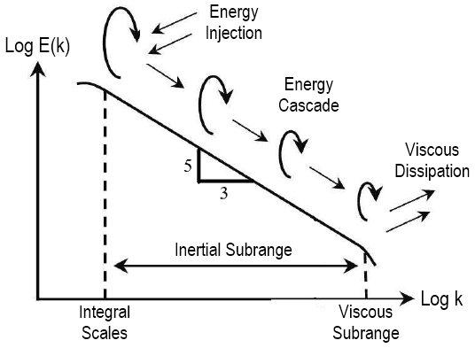
The CBL condition is ideal to study the small-scale turbulence and the high-frequency response of the sensors by means of power spectrum and structure function analysis. The energy cascade theory formulated by Kolmogorov is well proven (Kolmogorov, 1941) that can be used to estimate the turbulence energy distribution over a range of spatial scales under locally isotropic conditions. In one of the largest experiments conducted by Saddoughi and Veeravalli (1994), it was shown that in a turbulent atmosphere with a high Reynolds number the energy cascade decreases with a $-\mathrm{5}/\mathrm{3}$ slope in a logarithmic scale and then tails off downwards in the viscous dissipation region (Fig. 1). The approximate relation between the turbulence energy Φ_T of temperature and the spatial wavenumber k of the temperature signal is given by Tatarskiy and Silverman (1961):

$$\begin{array}{}\text{(1)}& {\mathrm{\Phi }}_{\mathrm{T}}\left(k_{\mathrm{1}}\right)\approx \mathrm{0.25}{C}_T^{\mathrm{2}}{k}^{-\mathrm{5}/\mathrm{3}},\end{array}$$

where C_T is the structure function parameter for temperature. The humidity also has a similar expression as Eq. (1) but with a different proportionality constant. Assuming the volume of air sampled by the UAS is locally isotropic, then the thermo-hygrometer sensors should observe a pattern similar to the $-\mathrm{5}/\mathrm{3}$ slope line. Assuming that the frequency content of the atmospheric eddies are larger than the frequency range that the sensor can capture, then any deviation in the sensor–data spectrum was assumed to be influenced by undesired sensor dynamics or noise.

Figure 1 Kolmogorov's energy cascade illustration.

Moreover, the Reynolds number Re of the PBL is typically on the order of 10⁶, and the ratio between large and small spatial scales is given by $l/\mathit{\eta }={\mathit{Re}}^{\mathrm{3}/\mathrm{4}}$. The large separation of scales allows for the inertial subrange (ISR) of turbulent fluctuations to extend for hundreds of meters in length, which would be quite difficult to cover with a UAS within a reasonable time. A workaround to this is to consider horizontally homogeneous CBL conditions. Consequently, the turbulence can be assumed to be “frozen” as it travels across a stationary UAS with mean wind speed relative to the UAS. This assumption is the so-called Taylor hypothesis of the frozen field, and it is of great use in calculating structure functions by converting temporal measurements into spatial measurements.

The definition of the structure function can be found in a vast amount of the literature (Gibbs et al., 2016; Kaimal et al., 1976; Kohsiek, 1982). The physical interpretation of structure function is the distribution of turbulent energy over different spatial lags, and it is mathematically defined as a two-point spatial correlation as follows:

$$\begin{array}{}\text{(2)}& D_{\mathrm{T}}^{\mathrm{2}}\left(r\right)=\stackrel{\mathrm{‾}}{\left(T\right(x)-T(x+r){)}^{\mathrm{2}}}=C_T^{\mathrm{2}}{r}^{\frac{\mathrm{2}}{\mathrm{3}}},\end{array}$$

where the overbar represents ensemble averaging, x is the position vector in meters, and r is the separation distance between two samples in space, also called distance lag. If the distance lag r is within the ISR, then the structure function is reduced to the rightmost expression of Eq. (2). In the ISR region, the structure function follows a $\mathrm{2}/\mathrm{3}$ slope line in a logarithmic scale. The computation of the structure function is straightforward and has relatively fewer theoretical assumptions than the conventional spectral analysis (Gibbs et al., 2016). Therefore, the structure function was considered as an extra step in the validation of the thermo-hygrometer observations and dynamical analysis.

For the case of FTIs, the PBL undergoes a quick evolution with strong gradients over a short time period in which large-scale changes in temperature and humidity are dominant over small scales. This is a good scenario for studying the low-frequency response of the sensors when flown across the air mass boundaries. Therefore, for this project, the main focus was to create artificial weather signals with strong gradients similar to that of FTIs without much importance on small-amplitude and high-frequency features. Temperature and humidity changes across a frontal or thermal inversion can be approximated to a ramp function with rounded corners.

3 Weather sensor principle and modeling

The performance optimization of the sensor starts with the available manufacturing technologies according to Farahani et al. (2014). Nowadays, the fabrication of sensors is driven by low-cost circuits, new sensing materials, advances in miniaturization techniques, and modern simulations. Despite the fact that a great part of the performance of the sensor can be optimized at a hardware level, they still come with limitations. Post-processing algorithms can partially overcome these limitations in performance, with modeling techniques and digital signal processing being the most popular. Dantzig (1985) showed encouraging first results using a simple first-order differential equation to restore signals from a thermocouple and even describing calibration procedures. Fatoorehchi et al. (2019) used nonlinear differential equations based on the Steinhart and Hart (1968) equation for negative temperature coefficient (NTC) thermistors. Their equations were comprised of a lumped formulation for temperature which also included other factors like thermal radiation and power dissipation. Despite its high accuracy, the high complexity of the model and solution makes it unpractical for real-time implementation. Moreover, Greene et al. (2019) have shown us that a good shielding around the sensors and an adequate sensor placement on the UAS can greatly prevent solar radiation and heat conduction from contaminating the sampled volume of air. Therefore, for this study, the external sources of contamination are considered negligible compared to the errors introduced by the internal sensor dynamics.

Wildmann et al. (2014b) used a similar approach and showed an example of the modeling of a capacitive humidity sensor using the diffusion equation and effectively applying an inverse model to correct the measurements. We were able to reproduce their modeling methods and validate the results with similar simulation experiments. Given the simplicity of this method, ideas from studies of Wildmann et al. (2014b) were borrowed to develop the IDMP proposed in this study, and it also served as a guidance to develop an IDMP variant for the bead thermistor. We also realized that a stability analysis with parameter tuning of the models, shown in Sect. 6.2, would be a great complement to their studies and a necessary tool for correct application of the IDMP.

3.1 Basics of temperature and humidity sensors

Commonly used temperature and humidity sensors for UASs are mainly variants of the bead thermistor type and capacitive type sensors, respectively (Barbieri et al., 2019; Kral et al., 2018). These type of sensors are considered payload friendly for small UASs given their compact size and lightweight characteristics. Both of these temperature and humidity sensors work under very similar principles. Basically, the heat flux (diffusion) inside the sensor's material will lead to a thermal (water vapor concentration) equilibrium with the surrounding medium after a finite time. In fact, the differential equation that describes most of their behavior has the exact same form for both sensors which is given by Pletcher et al. (2013):

$$\begin{array}{}\text{(3)}& {\displaystyle \frac{\partial U}{\partial t}}=k\left({\displaystyle \frac{{\partial }^{\mathrm{2}}U}{\partial x^{\mathrm{2}}}}+{\displaystyle \frac{{\partial }^{\mathrm{2}}U}{\partial y^{\mathrm{2}}}}+{\displaystyle \frac{{\partial }^{\mathrm{2}}U}{\partial z^{\mathrm{2}}}}\right).\end{array}$$

This is called the heat equation for the case of temperature and diffusion equation for the case of water vapor concentration. Farahani et al. (2014) explain that numerous parameters have an influence on the response time of a sensor, such as the geometry of the sensing element, the inherent thermal/water diffusivity of the sensing element, the thickness of the protective layers, and even the ambient temperature and humidity itself. Equation (3) encompasses most of these characteristics and factors and hence can be effectively used as a model to compensate for errors.

In particular, the selected sensors for this study are the iMet-XF bead thermistor from InterMet Systems and the HYT-271 capacitive humidity sensor from Innovative Sensor Technology (IST). This is for the sake of providing an example case with known sensor characteristics and specifications, and the overall modeling and method description does not lose its generality. Additionally, it is assumed the sensors are sufficiently aspirated (airflow of >5 m s⁻¹) as per the recommendation of the manufacturers so that self-heating effects are diminished.

3.2 Sensor dynamic modeling

In control theory, the method of finite difference is a commonly used numerical solution for differential equations and it is the main foundation of the IDMP method. Finite difference equations are powerful tools that can be used to create mathematical models to describe the behavior of physical systems. The method is an approximation of the derivative which is represented by the derivative taken over a finite interval around a given point. Additionally, assumptions must be made to reduce the complexity of the model and work within a linear regime. The dynamics of the sensor can be further studied after deriving the mathematical model. It can be used to trace back and restore the original signal that produced the sensor measurements as long as the inverse of the model exists and is stable.

3.2.1 Forward model of temperature sensor

The iMet-XF bead thermistor shape and dimensions are shown in Fig. 2, and the probe tip can be approximated to the shape of a sphere with radius R=0.4 mm. Given that heat fluxes can propagate anywhere around the sensor, the problem becomes three-dimensional in space. The spherical symmetry helps to significantly reduce the degree of complexity of the model to a one-dimensional case along the radius (Momoh et al., 2013). It was assumed that the heat propagates radially from the surface of the spherical glass in contact with the air all the way down to the core where the sensing element is located. Therefore, the problem can be seen as a heat transfer problem with spatial temperature gradients inside the bead thermistor. Accordingly, the differential equation for the bead thermistor is given by Eq. (3) in spherical coordinates:

$$\begin{array}{}\text{(4)}& {\displaystyle \frac{\partial T(r,t)}{\partial t}}=\mathit{\alpha }\left({\displaystyle \frac{{\partial }^{\mathrm{2}}T}{\partial r^{\mathrm{2}}}}+{\displaystyle \frac{\mathrm{2}}{r}}{\displaystyle \frac{\partial T}{\partial r}}\right),\mathrm{0}\le r\le R,t\ge \mathrm{0},\end{array}$$

where the internal temperature T is a function of time t and space r which is the radial distance from the center to a given point within the sphere, and α is the thermal diffusivity of the material. The boundary conditions are $T(R,t)=T_{\mathrm{air}}$ and T(0,t) is mirrored. The sphere was then divided into N layers with thickness $\mathrm{\Delta }r=R/N$. A finite difference method was applied to the spatial derivatives of Eq. (4), and the singularity at r=0 was solved by using L'Hôpital's rule. The following system of finite difference equations in space was obtained:

$$\begin{array}{}\text{(5)}& {\displaystyle }\begin{array}{rl}& {\displaystyle \frac{\partial T}{\partial t}}=\mathit{\beta }\left(-\mathrm{2}{T}_N+{\displaystyle \frac{N-\mathrm{1}}{N}}{T}_{N-\mathrm{1}}\right)+\mathit{\beta }{\displaystyle \frac{N+\mathrm{1}}{N}}{T}_{\mathrm{air}},\\ & r=R,\end{array}\text{(6)}& {\displaystyle }\begin{array}{rl}& {\displaystyle \frac{\partial T}{\partial t}}=\mathit{\beta }\left({\displaystyle \frac{i+\mathrm{1}}{i}}{T}_{i+\mathrm{1}}-\mathrm{2}{T}_i+{\displaystyle \frac{i-\mathrm{1}}{i}}{T}_{i-\mathrm{1}}\right),\\ & \mathrm{0}<i\mathrm{\Delta }r<R,i=\mathrm{2},\mathrm{\dots },N-\mathrm{1},\end{array}\text{(7)}& {\displaystyle \frac{\partial T}{\partial t}}=\mathrm{3}\mathit{\beta }\left(T_{\mathrm{2}}-T_{\mathrm{1}}\right),r=\mathrm{0},\end{array}$$

where $\mathit{\beta }=\mathit{\alpha }/\mathrm{\Delta }{r}^{\mathrm{2}}$. A more detailed derivation of these equations can be found in Momoh et al. (2013). As a result, the system of equations is a linear time invariant (LTI) system that can be transformed to the state–space representation of the following form:

$$\begin{array}{}\text{(8)}& {\displaystyle \frac{\partial x}{\partial t}}=\mathbf{A}x+\mathbf{B}u,\text{(9)}& {\displaystyle }y=\mathit{C}x+\mathbf{D}u,\end{array}$$

where x values are the state variables, each one representing the temperature at each layer, u is the surface temperature input signal, and y is the sensor's output signal (sensor reading or measurement at the core). The matrices A and B can be easily obtained by inspection from the finite difference equations.

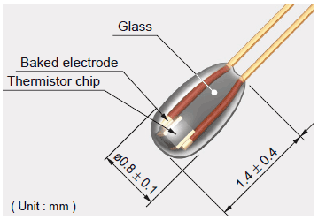
Figure 2 Closeup of the iMet-XF bead thermistor with dimensions and composition. Image provided by International Met (InterMet) Systems.

The goal is to determine the actual temperature of the medium based on temperature readings at the core. By computing the inverse model it is possible to trace back the temperature at each layer from the core to the surface of the sensor in a stable manner. In order to do so, the C vector must be a weighted average skewed towards the core. The D matrix was chosen in a way so that the DC gain (K) of the system is equal to one: $K=\mathbf{D}-\mathit{C}{\mathbf{A}}^{-\mathrm{1}}\mathbf{B}=\mathrm{1}$.

3.2.2 Forward model of humidity sensor

In the case of the HYT-271 capacitive humidity sensor, the dynamics are mainly produced by the diffusion of water vapor concentration from the surface in contact with the air into the polymer. Figure 3 shows the sensing element configuration and the boundary conditions around it. In contrast to the bead thermistor, the capacitive sensor can be treated as a one-dimensional problem since the water vapor only exists just above the sensing element surface, and it propagates along the normal to the surface.

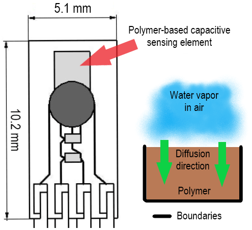
Figure 3 Closeup of the IST HYT-271 capacitive sensor with dimensions (left) and sensing element configuration (right). Left image taken from datasheet.

Horizontal concentration gradients were considered to be negligible given that the thickness of the polymer is small enough to prevent horizontal propagation (Wildmann et al., 2014b). As a result, the differential equation for the capacitive humidity sensor is given by Eq. (3) in one-dimensional Cartesian coordinates:

$$\begin{array}{}\text{(10)}& {\displaystyle \frac{\partial c(x,t)}{\partial t}}=D{\displaystyle \frac{{\partial }^{\mathrm{2}}c}{\partial x^{\mathrm{2}}}},\mathrm{0}\le x\le L,t\ge \mathrm{0},\end{array}$$

where c is the water vapor concentration in parts per million volume (ppmv), D is the diffusivity coefficient of the water vapor in the polymer, and L is the thickness of the polymer. The boundary conditions were defined as $c(L,t)=c_{\mathrm{air}}$, while c(0,t) is mirrored. The polymer film was then divided into N layers with thickness $\mathrm{\Delta }x=L/N$. Following a similar reasoning and steps as applied with the bead thermistor model, the system of finite difference equations is as follows:

$$\begin{array}{}\text{(11)}& {\displaystyle \frac{\partial c}{\partial t}}=\mathit{\lambda }\left(-\mathrm{2}{c}_N+c_{N-\mathrm{1}}\right)+\mathit{\lambda }{c}_{\mathrm{air}},x=L,\text{(12)}& {\displaystyle }\begin{array}{rl}& {\displaystyle \frac{\partial c}{\partial t}}=\mathit{\lambda }\left(c_{i+\mathrm{1}}-\mathrm{2}{c}_i+c_{i-\mathrm{1}}\right),\\ & \mathrm{0}<i\mathrm{\Delta }x<L,i=\mathrm{2},\mathrm{\dots },N-\mathrm{1},\end{array}\text{(13)}& {\displaystyle \frac{\partial c}{\partial t}}=\mathit{\lambda }\left(c_{\mathrm{2}}-c_{\mathrm{1}}\right),x=\mathrm{0},\end{array}$$

where $\mathit{\lambda }=D/\mathrm{\Delta }x$. A more detailed derivation of the above equations can be found in Wildmann et al. (2014b). Again, the resulting system of equations is an LTI system that can be transformed to the state–space representation. The matrices A and B can be determined by inspection from the finite difference equations. The output y of the system is equal to the average of all the water vapor concentrations in each layer. This is because the capacitance is measured across the entire polymer film and not just one particular spot as compared to the bead thermistor. Therefore, the parameter C is a length N row vector with elements equal to $\mathrm{1}/N$, and it maps the state variables to the output resulting in the sensor measurement.

The HYT-271 humidity sensor comes hard-coded to output relative humidity values. The model only works with water vapor concentration in parts per million volume (ppmv) units. Therefore, the relative humidity input must be converted to water vapor concentration and then back to relative humidity after applying the model. The following equations for the conversion were taken from McRae (1980), who states that the error involved in using these equations over a temperature range of −50 and 50 ^∘C is less than 0.5 %:

$$\begin{array}{}\text{(14)}& {\displaystyle }c={\mathrm{10}}^{\mathrm{4}}H{\displaystyle \frac{P_{\mathrm{s}}}{P_{\mathrm{a}}}},\text{(15)}& {\displaystyle }\begin{array}{rl}{P}_{\mathrm{s}}& =P_{\mathrm{a}}\exp \left(\mathrm{13.3185}t-\mathrm{1.9760}{t}^{\mathrm{2}}-\mathrm{0.6445}{t}^{\mathrm{3}}\right.\\ & \left.-\mathrm{0.1299}{t}^{\mathrm{4}}\right),\end{array}\text{(16)}& {\displaystyle }t=\mathrm{1}-{\displaystyle \frac{\mathrm{373.15}}{T_{\mathrm{a}}}},\end{array}$$

where H is relative humidity in percentage, P_s is saturation vapor pressure in millibars, P_a=1013.25 mb is the standard atmospheric pressure, and T_a is the ambient temperature in Kelvin.

4 Experimental design for sensor characterization

The geometry and boundary conditions were defined in the forward sensor models presented in Sect. 3.2. The sampling period of the sensor must also be known at this point; both iMet-XF and HYT-271 have sampling periods equal to Δt=0.1 s. The remaining parameters to be defined in the models are the thermal (or water) diffusivity α (or D), the width of the sensing material R (or L), and the thickness of the layers Δr (or Δx). Unfortunately, these parameters are usually not in the datasheet and even kept as a trade secret by the manufacturer. However, these parameters are associated with the time response of the model, and they can be adjusted to approximate the time response of the real sensor (Wildmann et al., 2014b). Therefore, the remaining parameters can be obtained empirically in the lab through experimentation. In addition, please note that the response time is defined as the time required for the sensor output to change from its initial state to a final fixed value within a tolerance, typically defined as 98 % of the final value.

In an effort to establish guidance for the sensor characterization of UASs, Jacob et al. (2018) conducted experiments in which weather UASs were flown across a pseudo-step change in temperature and humidity from an air conditioned room to the outdoor environment. Although their goal was to measure the sensor time response with the effects of the UAS on the sensors altogether, a different approach was taken for the presented study in which the problem was divided into two parts. First, the sensors were isolated and characterized independently of the UAS body through experimentation. Second, the sensor siting on the UAS and sampling techniques were investigated to minimize the external disturbances on the measurements.

Ideally, the time response is measured by stimulating the sensor with an ideal step function. However, step functions of temperature and humidity are not possible in real-world conditions. Instead, Li et al. (2018) used a ramp function to model the thermodynamic shock and found that the error of assuming an ideal step function is less than 10 % if the transition time from the initial to the final state is less than the time response of the sensor. According to the iMet-XF bead thermistor datasheet, the sensor response time can be less than 1 s. Therefore, it is a requirement to have a mechanism to quickly move the sensors from one side of the shock to the other.

There are several external factors that influence the physical aspects of the sensor that must be taken into account for the experiments. In particular, the capacitive humidity sensor is mainly affected by the ambient temperature as explained by Farahani et al. (2014). This is because the porosity and thickness of the sensor's polymer significantly changes with temperature. This means that there is no universal water vapor diffusivity D that can be used for a wide range of ambient temperature. Therefore, the shock experiments for the humidity sensor must be performed at different air temperature conditions to create a lookup table of values. After a UAS flight, the mean temperature of the profile can be used to determine the diffusivity value from the lookup table by interpolation. Conversely, the thermal diffusivity α of the bead thermistor does not significantly change with humidity as measured by Tsilingiris (2008). Consequently, only one shock experiment would be enough to compute a universal thermal diffusivity α for the bead thermistor.

After conducting the experiments for sensor characterization, the collected data are used to adjust the sensor model parameters by using a model parameter optimization technique called differential evolution (Das and Suganthan, 2011). Simulated step functions with amplitudes equal to the real thermodynamic shocks from the experiments are fed to the digital models with equal sampling rate as the real sensors. The model parameters can be initialized through a reasonable guess, and the subsequent parameters are computed by iterative point-wise comparisons with the real data. Basically, this becomes a curve fitting problem by minimizing the square root of the mean of the squared error (RMSE) cost function across the dataset:

$$\begin{array}{}\text{(17)}& \mathrm{RMSE}=\sqrt{{\displaystyle \frac{\sum {\left(U_{\mathrm{mod}}-U_{\mathrm{obs}}\right)}^{\mathrm{2}}}{N}}}<\mathit{ϵ},\end{array}$$

where U_mod is the predicted value of the model, U_obs is the real observation, N is the number of data points, and ϵ is the desired tolerance. The thermal (water vapor) diffusivity are slightly tweaked on every subsequent iteration until meeting the tolerance criteria and thus obtaining the final diffusivity coefficient for the given conditions.

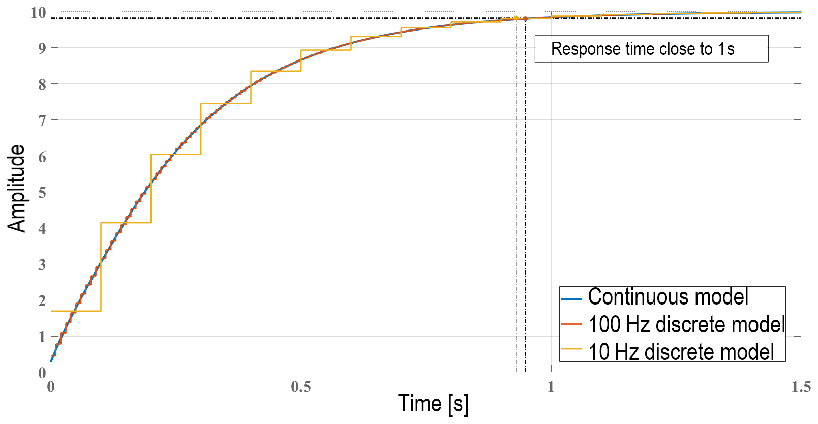
Finally, the sensor time response can be assessed quantitatively by examining the final RMSE value. If the RMSE value remains high after several iterations, it means that the sensor transient response is highly nonlinear compared to the linear model, and hence, a higher uncertainty in the measurement correction process is expected. Figure 4 shows an example of how the step response of the continuous and discrete models of a bead thermistor should look like with a response time close to 1 s. Notice how important it is to have a high sampling rate logger in order to accurately capture the dynamics of the sensor.

Figure 4 Step response of the continuous and discrete models of the bead thermistor.

5 Considerations for sensor placement on UAS

Acquiring precise measurements of the air temperature and humidity is particularly challenging due to disturbances arising from multiple sources around the UAS. Insufficient radiation shielding, exposure to mixed turbulent air from the propellers, and electronic self-heating are the main factors in contributing to temperature and humidity data contamination according to Greene et al. (2018, 2019) and Islam et al. (2019). A quick logical solution is to make an extension arm from the main body of the UAS and place the sensor package outside of the turbulent air created by the UAS. However, this approach comes with major problems such as increased resistance to rotation (or inertia) and exposure to strong aerodynamic forces that could produce flight instability. Therefore, the integrated design must be balanced in such a way that neither of the systems gets compromised.

The multi-rotor UASs are the most vulnerable platforms since they usually remain stationary in the air or travel at very low speeds (mainly vertical profiles), allowing for the turbulent air volume to wrap around the multi-rotor UAS. Greene et al. (2018) searched for the best-possible location for the thermodynamic sensors within the turbulent air volume. They measured variations in temperature right below a multi-rotor UAS propeller and found that disturbances were minimum at $\mathrm{1}/\mathrm{3}$ from the tip of the propeller. Despite the encouraging results, the study did not take into account the heat advection coming from the UAS body. Islam et al. (2019) took it a step further by mounting pipes with air inlets situated far apart from the main body while still using the multi-rotor UAS rotors to produce mechanical aspiration. They reported good agreement between ascent and descent profiles in no wind conditions but also showed limitations with the flight stability and heat advecting into the pipes downwind of the UAS. Segales et al. (2020) took an innovative approach by modifying the autopilot code to compute wind direction estimates and command the multi-rotor UAS to turn into the wind. In this way, the wind itself compresses the turbulent envelope in front of the multi-rotor UAS making it shallow enough to place the sensors closer to the multi-rotor UAS's body. This was demonstrated using flow simulations by Segales et al. (2020) and also through observations in the field by Greene et al. (2019) and Bell et al. (2020).

An important consideration that is common to both a multi-rotor UAS and a fixed-wing UAS is the material selection for the radiation shield around the weather sensors. Greene et al. (2019) have shown that the sun radiation greatly affects the temperature and humidity measurements. They noticed an unusual pattern in the readings during flights in a day with scattered clouds despite the multi-rotor UAS having a shield around the sensors. Basically, the sun radiation heats up the surface of the shield and, consequently, increases the temperature of the surrounding air by heat conduction. The heated air is then aspirated across the sensors. Waugh (2021) shows an example of a thorough radiation shield design, as well as a useful guide for sensor placement and installation. Moreover, materials with low thermal conductivity can help reduce heat conduction to the air and hence mitigate the contamination. For instance, aerogel can be a great candidate material that could almost completely isolate the sensors from the sun radiation. Also, radiant barrier paint can be used to coat the current shield designs and prevent surfaces from loading with heat.

6 Implementation of the IDMP

At this point, two models were introduced, one describing the bead thermistor sensor dynamics and another describing the capacitive humidity sensor dynamics. An experimental design for sensor characterization and model validation were also presented, and some of the limitations were reviewed. In an effort to reinforce the concepts just introduced and to demonstrate the actual implementation of the IDMP method, this section will fully describe the procedures of the IDMP for correcting sensor measurements.

6.1 General procedures and limitations

In order to detail and formulate the IDMP restoration technique, it will be beneficial to start by summarizing a basic general procedure, part of which is taken from Wildmann et al. (2014b):

1. Identify the sensor noise floor from the actual measurements by inspecting its power spectral density (PSD) and suppress the noise using a zero-phase low-pass filter.

2. Apply the inverse sensor model to the filtered measurements after adjusting the model parameters based on the weather conditions and sensor characterization.

3. Re-apply the filter from step 1 to the restored signal to filter out any amplified noise.

4. Quantify the improvement by inspecting the time series and spectral response of the signal before and after applying the inverse sensor model.

5. Validate the correction by comparing the structure function with the theoretical $\mathrm{2}/\mathrm{3}$ slope for locally isotropic turbulence in the ISR.

Although the general procedure seems to be robust in the sense that it includes a validation step, the validation step only works for CBL weather conditions as explained in Sect. 2. Furthermore, step 5 is feasible only if the atmosphere is assumed to be horizontally homogeneous and locally isotropic without any rapid atmospheric evolution. Additionally, the flight patterns are limited to steady hover in windy conditions and horizontal transects assuming Taylor's hypothesis of frozen field holds true. For the case of flights across FTIs, only steps 1 to 3 are feasible, and the results can be trusted based on prior testings and calibrations.

6.2 System description and tuning

The signal conditioning of the raw sensor measurements is necessary to extract a more accurate representation of the atmospheric parameters. The challenge is to remove the unwanted distortion and contamination caused by slow sensor dynamics and sensor noise, respectively. If the considerations from Sect. 5 are correctly implemented, then the effects of the UAS and its immediate surroundings on the sensor measurements are considered to be small and can be ignored. The type of low-pass filter chosen for noise removal was a non-causal zero-phase finite impulse response (FIR) digital filter. This kind of filter has the advantage that it does not introduce phase delay to the output signal with respect to the input signal, which is only possible in an offline processing.

An adaptive contamination removal algorithm was not developed for the IDMP method. Instead, the cut-off frequency of the low-pass filter was manually tuned on a case by case basis. The PSD of the raw sensor measurement was used to assess the dynamics of the sensor, identify the noise floor, and define the cut-off frequency of the low-pass filter. Moreover, the logic used to identify distortion and contamination in the measurements taken in CBL conditions is as follows:

• If the slope of the PSD is greater than $-\mathrm{5}/\mathrm{3}$ at high wavenumbers, then the region is considered to be contaminated by sensor noise. This is because of the natural downward trend of the turbulence power spectrum that eventually encounters the noise floor of the sensor. Therefore, it must be removed using the low-pass filter before going through the restoration phase to prevent the noise from getting amplified.

• Otherwise, the measurement is considered to be attenuated and distorted by the slow sensor dynamics which cannot keep up with the turbulence dynamics. Consequently, the bad trend is corrected in the restoration phase, and the new PSD approximates the desired $-\mathrm{5}/\mathrm{3}$ slope line.

The next step is to run the conditioned signal through the core of the IDMP method, the inverse sensor model itself. The transfer function H(z) of the sensor model was computed by taking the z transform of the state–space system of the sensor model. Figure 5 shows an example of the frequency response of the continuous and discrete transfer function H of a capacitive humidity sensor with a response time of about 4 s. The continuous system is the approximation to the analog behavior of the sensor and can be used to simulate the “real” sensing element. The discrete system is a “sampled” version of the continuous system with sampling rate equal to that of the real sensor or the analog-to-digital converter (ADC) to be precise. The truncation effect that comes with sampling a system is what produces the mismatch in the frequency response at high frequencies, which is seen in Fig. 5. The only way to improve the frequency response of the discrete system is by increasing the sampling rate of the ADC to better capture the dynamics of the sensing element.

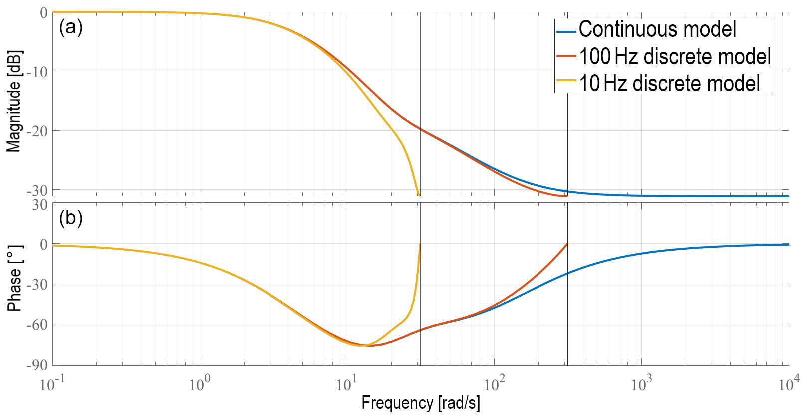
Figure 5 Bode diagram of the sensor model. Magnitude and phase are shown in panels (a) and (b), respectively.

The inverse system of H(z) exists, and it is stable if and only if H(z) is minimum phase, meaning that all the poles and zeros are within the unit circle of the z plane. Subsequently, the transfer function of the inverse sensor model is obtained by simply taking the inverse of $H\left(z\right)=G^{-\mathrm{1}}\left(z\right)$. Even though the process of finding the inverse sounds simple and straightforward, special attention must be given to the poles of G(z). The resulting poles of G(z) might end up being too close to the unit circle of the z plane which could cause instability and oscillations with high-frequency input signals. The stability parameter for the presented models is defined by Pletcher et al. (2013) as $\mathit{\varphi }=\frac{\mathit{\gamma }\mathrm{\Delta }t}{\mathrm{\Delta }{x}^{\mathrm{2}}}<\mathrm{0.5}$, where γ is an intrinsic parameter of the sensor, such as the thermal and diffusivity coefficients. The equation shows how fast the sampling rate must be in order to precisely capture the dynamics of the sensor within a small spatial interval. Given that the sampling rate of the sensors is fixed at Δt=0.1 s, then the only way to adjust the poles is by varying Δx. The model and hence its inverse G(z) are stable with large values of Δx at the expense of reducing the order of the model and, consequently, the overall accuracy and resolution of the method. Moreover, notice that the degree of correction made on the sensor measurements is limited by the sensor's sampling rate. If the same sensors are enabled to sample at higher rates, then the IDMP will become more effective.

After tuning the parameters and creating a stable system, G(z) was then fed with the filtered sensor measurements to produce the corrected sensor measurement. Finally, the same low-pass filter from the beginning was applied to the corrected signal to remove any amplified noise that survived the process.

7 Performance evaluation of the IDMP

The first step to investigate the potential of applying the IDMP for temperature and humidity measurements is to develop a time-series weather signal generator that could be used as a benchmark to evaluate the performance of the proposed framework. From this point, signals made by the generator will be referred to as “actual” weather signals, whereas the output signals from the sensor models will be referred to as the “measured” signal, and the restored signals from the IDMP will be called “corrected” signals.

7.1 Weather signal generation and sensor simulation

As described in Sect. 2, CBL weather signals from a horizontal transect tend to have a particular PSD with a $-\mathrm{5}/\mathrm{3}$ slope in the logarithmic scale. Moreover, assuming horizontal CBL weather signals are produced by a wide-sense stationary (WSS) random process with Gaussian probability density function, then it is possible to generate the artificial weather signals by modifying the PSD of a Gaussian white noise signal to look like Kolmogorov's energy cascade power spectrum. This was achieved by taking the Fourier transform of a white noise signal and dividing the magnitude by its frequency to the power of $\mathrm{5}/\mathrm{6}$ while keeping the phase unchanged. Figure 6 shows an example of an artificially generated CBL weather signal.

Figure 6 Spatial temperature signal in CBL conditions after converting the time-series data given a constant wind speed of 10 m s⁻¹.

For the case of FTI conditions, the focus is mainly on the evaluation of the sensor response in strong gradients with less importance on features with small amplitude and high frequency. Therefore, the FTI weather signals were constructed in a piece-wise manner using straight lines. The horizontal transect of an FTI was modeled using a ramp function, whereas the vertical transect follows a dry adiabatic lapse rate model with a temperature inversion in the middle. Both weather signals were low-pass filtered to smooth out the corners so that it looks more realistic. The gradient (or inversion) strengths, length, and altitude scales of the weather signals were adjusted using the simulation results shown by Houston and Keeler (2018) as a reference. Figure 7 shows examples of generated FTI weather signals.

Figure 7 (a) Temperature change across a frontal inversion (cold front). (b) Vertical dry adiabatic lapse rate temperature profile with a strong thermal inversion.

To simulate the sensor measurement process, the sensor model was divided into three parts: the analog sensing element, the ADC discrete sampling, and sensor noise generation. The sensing element was simulated using the forward models shown in Sect. 3.2 with a much smaller sampling period Δt=0.01 s. This is because analog signals can not be generated in a computer, and, therefore, the best approximation is to increase the resolution of the discrete model. The actual weather signal was run through the high-resolution sensor model to add the effects of sensor dynamics. This signal then goes through the ADC which down-samples the signal to the actual sampling period of the sensor Δt=0.1 s. The down-sampling process may add aliasing which makes it more realistic. Finally, the down-sampled signal gets its characteristic noise floor by adding additive white Gaussian noise (AWGN) to it. The noise amplitude from each sensor was taken from previous steady-state calibrations done in a controlled environment by the Center for Autonomous Sensing and Sampling (CASS) of the University of Oklahoma.

7.2 Validation of the IDMP method in simulated CBL conditions

The following measurement validation method for CBL conditions exploits the ISR of turbulent fluctuation theory, described in Sect. 2, by using the PSD and structure function calculations. In real-world CBL conditions, the data are collected by conducting horizontal transects or stationary flights in windy conditions at a constant altitude with a multi-rotor UAS. In order to keep this article short and because the correction results of temperature and humidity are very similar, results will be shown in an alternated fashion between temperature and humidity.

Following the procedures of the IDMP from start to end, the PSDs of the signals are computed and compared in Fig. 8. Notice that the cut-off frequency of the low-pass filter was selected near the constant and flat power level of the measured signal, and the sensor noise was effectively removed as a result. The effect of the slow sensor dynamics is noticeable as a downward trend with respect to the $-\mathrm{5}/\mathrm{3}$ slope line. The IDMP successfully restores the power levels of the measured signal at high frequencies. Next, Fig. 9 shows a comparison of the time-series signals, and the RMSE of the measured and corrected signals were computed with respect to the actual weather signal using Eq. (17). The time-series plot clearly shows an improvement in the time response of the sensor which is confirmed by the lower RMSE value. Finally, Fig. 10 shows results from the two-point spatial correlation calculation, namely, the structure function. Assuming locally isotropic turbulence conditions, the deviations of the computed structure function from the theoretical $\mathrm{2}/\mathrm{3}$ slope in the ISR region are indications of the effects of sensor dynamics and sensor noise on the measurement. Moreover, the results can be used to slightly tune the IDMP until getting a best-possible agreement with the theory. Additionally, all the presented results show that the IDMP method is effectively restoring the signal without any signs of instability and oscillations.

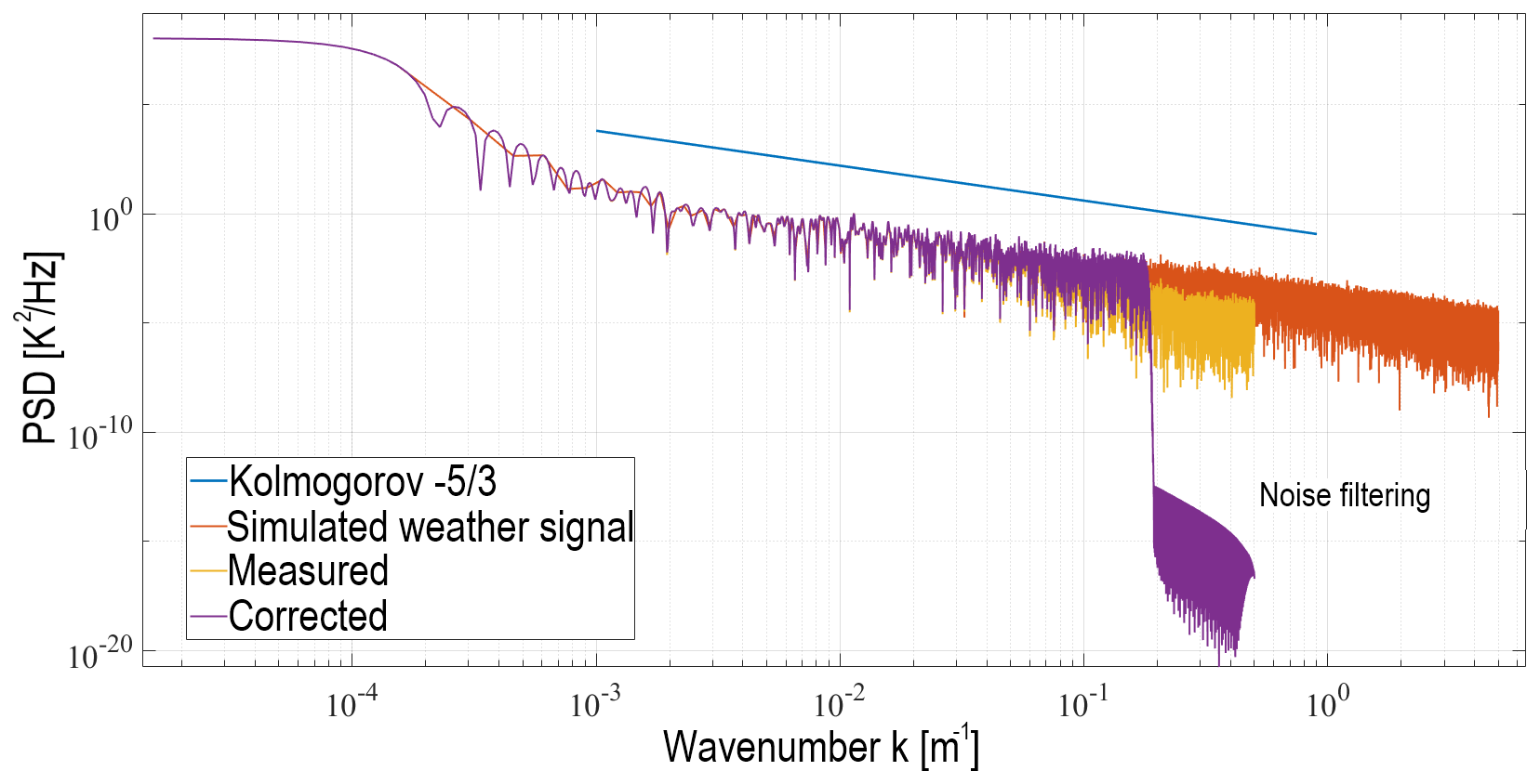
Figure 8 Power spectral density of the simulated weather signal in CBL conditions and processed signals using the sensor models. Results from before and after applying the IDMP are shown.

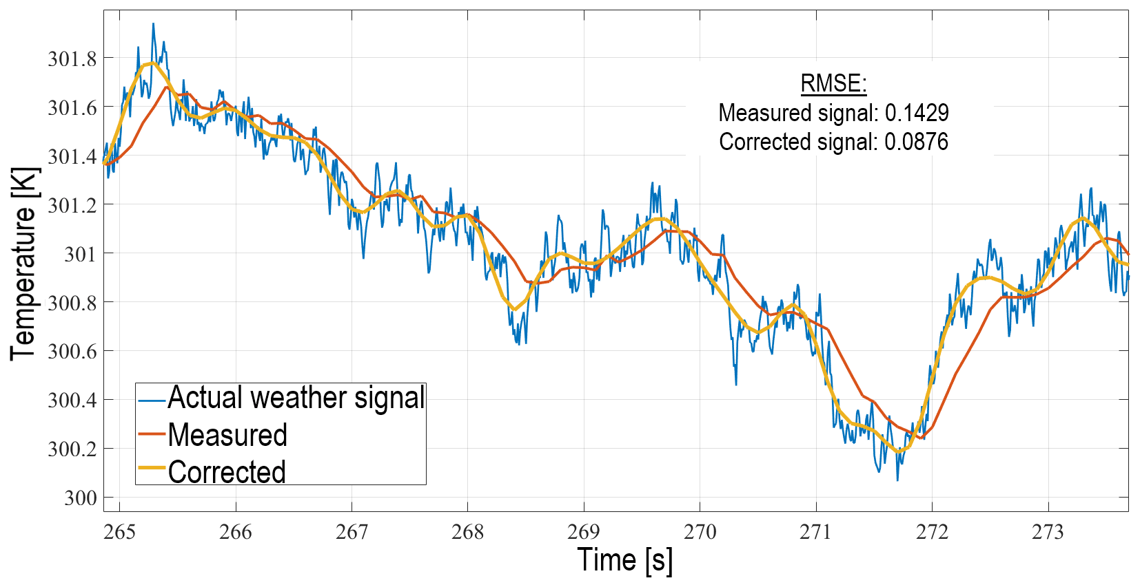
Figure 9 Time series of the simulated weather signal in CBL conditions and processed signals using the sensor models. Results from before and after applying the IDMP are shown.

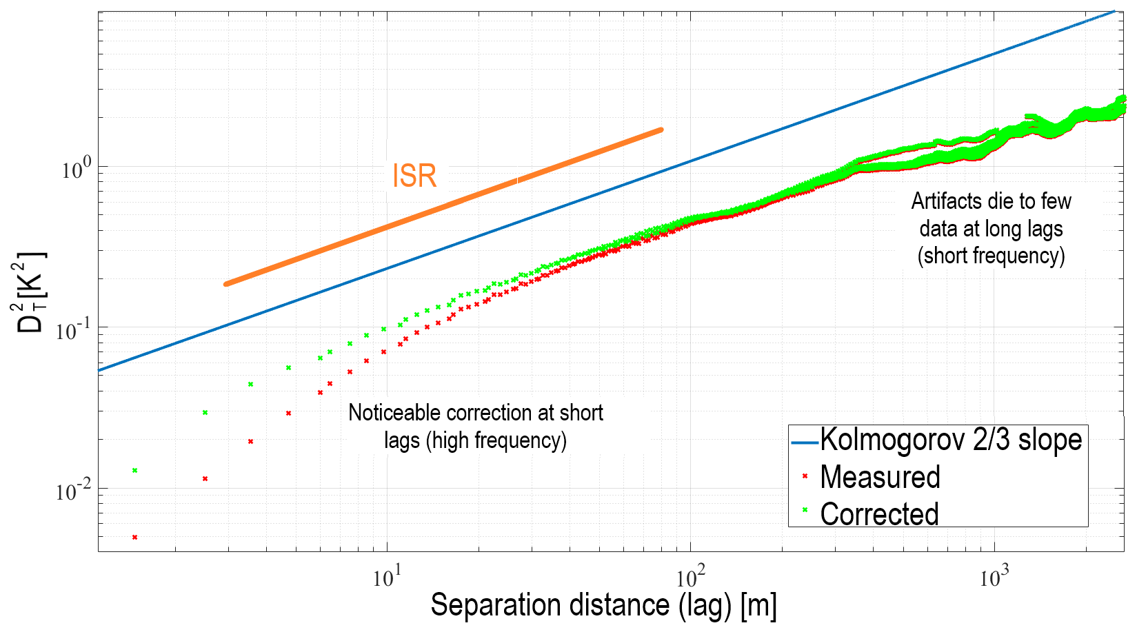
Figure 10 Structure function of the simulated weather signal in CBL conditions and processed signals using the sensor models. Results from before and after applying the IDMP are illustrated.

7.3 Simulation of flights across strong gradients in FTI conditions

Similar to the CBL simulation, flights across FTIs also exhibit the expected lag in the measurement as a consequence of the sensor time response. Additionally, the lag within this condition becomes more apparent and sensitive to the relative wind speed with respect to the UAS. Houston and Keeler (2018) explain that the number of errors is fewer when flying at low speeds; however, the observation might not be representative because the weather phenomena might have evolved faster than the observation period. Therefore, it is of significant importance to study the performance of the IDMP method with different speeds across the thermodynamic boundary. For the case of frontal inversions, results from the simulated humidity sensor will be shown since it has a large time response, and the correction is more noticeable compared to the faster temperature sensor, whereas for the thermal inversion, results from the simulation of the temperature sensor will be shown.

Frontal inversions, such as cold fronts, are usually sampled using a fixed-wing UAS. The typical ground speed of a fixed-wing UAS in flight is around 25 m s⁻¹, while the wind can reach speeds of 20 m s⁻¹. Assuming that the fixed-wing UAS is able to fly in very windy conditions, then the relative wind across the fixed-wing UAS is 45 m s⁻¹ when flying into headwinds. It has to be mentioned that such an airspeed is extremely high for a typical fixed-wing UAS. However, testing the IDMP outside the operating envelope of the UAS is a good way to show its robustness. Figure 11a shows the comparison between the actual, measured, and corrected humidity in a frontal inversion. Notice how far the measured signal settles with respect to the air mass boundary; this agrees with the results seen in Houston and Keeler (2018). The corrected signal shows a much better transient response, but some oscillations are present when the weather signal is constant. This is because of some remaining sensor noise leaking into the IDMP where it gets slightly amplified. Additionally, the IDMP can not fully recover the shape of the actual weather signal because of missing parts in the frequency content due to noise filtering, low sampling rate, and poor capturing of the weather dynamics.

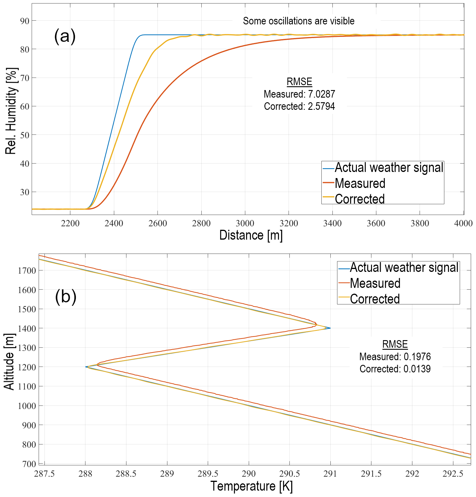
Figure 11 Comparison of weather signals in simulated (a) frontal inversion conditions with relative wind speed of 45 m s⁻¹ and (b) thermal inversion conditions with climbing rate set to 5 m s⁻¹. Results from before and after applying the IDMP are illustrated.

Vertical profiles are typically carried out using a multi-rotor UAS, and it is common to encounter thermal inversions aloft. The vertical speed of the multi-rotor UAS was assumed to be equal to the radiosonde's climbing speed of about 5 m s⁻¹, much slower compared with the horizontal speed of a fixed-wing UAS. Figure 11b illustrates a comparison between signals in the simulated thermal inversion environment. It can be seen that the IDMP corrects for the constant offset produced by the sensor dynamics not being able to keep up with the temperature change rate. Once the multi-rotor UAS encounters the inversion, the result is almost identical to the frontal inversion case.

7.4 Case study using real data

The presented simulation results show the feasibility of the framework and the IDMP technique on measurements taken with a UAS. However, several assumptions were made to produce the models and simulations which may not hold true for real observations in the field. Therefore, to begin exploring the mitigation of slow sensor dynamics and sensor noise for realistic UAS flights, the IDMP was applied on real data collected using the CopterSonde UAS (Segales et al., 2020) from the University of Oklahoma (OU). Two flights were picked from the extensive database made in the past years throughout several field campaigns. Although these two flights are not available in an open online repository, a similar dataset can be found in Greene et al. (2020) and described in Pillar-Little et al. (2021) which was collected with the same UAS in this study.

These flights were conducted in CBL and FTI weather conditions, respectively, at the Kessler Atmospheric and Ecological Field Station (KAEFS) in Purcell, Oklahoma, USA, located 30 km southwest of the OU Norman campus. The Certificate of Authorization (COA) with number 2020-CSA-6030-COA, issued by the Federal Aviation Administration (FAA), allowed us to fly the CopterSonde above 122 m (400 ft) with a flight ceiling of 1524 m (5000 ft). It has to be mentioned that the sensors were not properly characterized as described in the presented literature; instead the sensor models were tuned by trial and error and best guessing the physical parameters of the sensing elements. Although the sensor characterization was poor, the implementation still showed the potential benefits of using the IDMP.

In the CBL conditions, the CopterSonde was flown stationary at a constant altitude of 10 m for about 15 min with a mean wind speed of 10.2 m s⁻¹. Figure 12a shows a close-up of a portion of the measured and corrected relative humidity time series, while Fig. 12b illustrates the degree of correction made by the IDMP. This is noticeable by observing the amount of deviation in the structure function.

Figure 12 (a) Comparison of the measured against corrected relative humidity signal. (b) Structure function comparison.

In the FTI conditions, the CopterSonde was flown shortly after a cold front moved through KAEFS, leaving a shallow cold pool behind. The climbing rate was set to 3.5 m s⁻¹, whereas the descent rate was set to 5 m s⁻¹. The CopterSonde was sent to 1300 m above ground level, collecting temperature and humidity data in the ascent and descent legs. The flight took about 10 min from take-off to landing. Figure 13a shows a comparison between the measured and corrected vertical profiles of relative humidity. The correction is not very noticeable due to the large spatial scale and the slow vertical speed of the UAS. However, Fig. 13b is a zoomed-in plot of the lower altitude region where the small correction is visible. Assuming that no other environmental factors influenced the measurements, this may confirm that the separation shown by the arrow is in fact an atmospheric evolution and not a result of sensor lag.

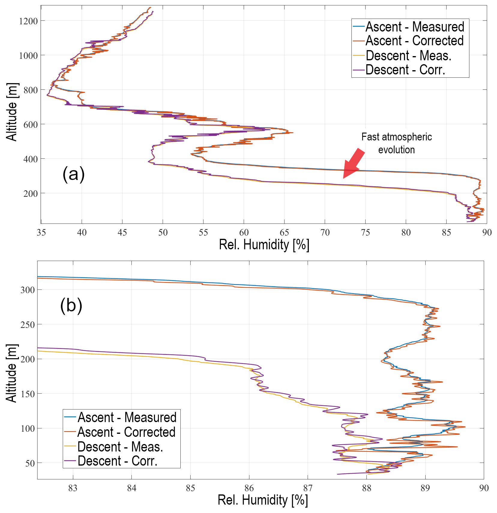
Figure 13 (a) Relative humidity vertical profile measured against corrected values. (b) Close-up of the vertical profile in the lower altitude region.

8 Conclusions

This article presented an overview of the general procedures for the mitigation of undesired sensor dynamics on temperature and humidity measurements collected using a UAS. Important considerations about the effects of the UAS on the sensor measurements were shown, in which it is encouraged to find solutions that benefit both flight stability and weather sampling accuracy.

Furthermore, sensor models were developed to investigate the sensor transient response, and a collection of best practices for sensor characterization and installation was presented to ensure reduced contamination of the air sample. This allowed for the design and implementation of signal restoration techniques under adequate conditions, such as the IDMP shown in this study. The authors also took it a step further and studied the stability of the sensor models and the IDMP method. A system tuning criterion was presented which helped determine the operating envelope of the IDMP and its limitations. This same analysis could be used as leverage for finding improvements within the sensor model design and the sensor selection for the desired application.

After a brief review of the PBL theory, ways have been found to create a correction criterion based on the power spectrum density calculation. As a result, the sensor measurements were corrected in a way that the resulting power spectrum was more consistent and aligned to Kolmogorov's power spectrum theory under locally isotropic assumptions. The structure function was then used as a mean to corroborate the corrections which gave some degree of validation to the results. The simulation results served as good evidence for this criterion in which the mitigation of undesired contamination and signal restoration using the IDMP was found to be significant in improving the reliability of the weather UAS deliverables when flying across strong thermodynamic gradients.

Finally, the case study demonstrated the feasibility of using the IDMP outside of the ideal and simulated conditions. The IDMP remained stable throughout both flights while also making small sensor response corrections in the time domain, which is more noticeable in the frequency domain where it follows the $\mathrm{2}/\mathrm{3}$ slope more consistently. Despite these achievements, the case study does not provide enough material to fully support the use of the IDMP for sensor measurement correction. However, the case study is considered to be a good trend towards producing weather signals with richer frequency content relative to Kolmogorov's theory that can lead to a better understanding of the atmosphere's structure.