the Creative Commons Attribution 4.0 License.
the Creative Commons Attribution 4.0 License.
 | 06 May 2022
Exploiting Aeolus level-2b winds to better characterize atmospheric motion vector bias and uncertainty
Katherine E. Lukens
Kevin Garrett
David Santek
Brett Hoover
Ross N. Hoffman
The need for highly accurate atmospheric wind observations is a high priority in the science community, particularly for numerical weather prediction (NWP). To address this need, this study leverages Aeolus wind lidar level-2B data provided by the European Space Agency (ESA) as a potential comparison standard to better characterize atmospheric motion vector (AMV) bias and uncertainty. AMV products from geostationary (GEO) and low Earth orbiting (LEO) satellites are compared with reprocessed Aeolus horizontal line-of-sight (HLOS) global winds observed in August–September 2019. Winds from two Aeolus observing modes are compared with AMVs, namely Rayleigh-clear (RAY; derived from the molecular scattering signal) and Mie-cloudy (MIE; derived from the particle scattering signal). Quality-controlled (QC'd) Aeolus winds are co-located with QC'd AMVs in space and time, and the AMVs are projected onto the Aeolus HLOS direction. Mean co-location differences (MCDs) and the standard deviation (SD) of those differences (SDCDs) are determined and analyzed.
As shown in other comparison studies, the level of agreement between AMV and Aeolus wind velocities (HLOSVs) varies with the AMV type, geographic region, and height of the co-located winds, as well as with the Aeolus observing mode. In terms of global statistics, QC'd AMVs and QC'd Aeolus HLOSVs are highly correlated for both observing modes. Aeolus MIE winds are shown to have great potential value as a comparison standard to characterize AMVs, as MIE co-locations generally exhibit smaller biases and uncertainties compared to RAY co-locations. Aeolus RAY winds contribute a substantial fraction of the total SDCDs in the presence of clouds where co-location/representativeness errors are also large. Stratified comparisons with Aeolus HLOSVs are consistent with known AMV bias and uncertainty in the tropics, NH extratropics, the Arctic, and at mid- to upper-levels in clear and cloudy scenes. AMVs in the SH/Antarctic generally exhibit larger-than-expected MCDs and SDCDs, most probably due to larger AMV height assignment errors and co-location/representativeness errors in the presence of high wind speeds and strong vertical wind shear, particularly for RAY comparisons.
- Article
(9669 KB) - Full-text XML
- BibTeX
- EndNote


Improving atmospheric 3D wind observations in the troposphere has long been a high priority in the science community. In 2018, the National Academies Press published the 2017–2027 decadal survey for Earth science and applications from space (National Academies of Sciences, Engineering, and Medicine, 2018) that included 3D winds in a series of observation requirement priorities and accompanying recommendations. The survey found that radiometry-based atmospheric motion vector (AMV) tracking should be an important approach to address the priority requirement of 3D winds.
AMVs are wind observations derived from tracking clouds and water vapor features in satellite images through time. Both geostationary (GEO) and polar-orbiting, i.e., low Earth orbiting (LEO), satellites observe the motion of such features in several spectral regions. Infrared bands that are specifically sensitive to water vapor (WV) absorption can capture different atmospheric motions using the same channel by tracking (1) upper-level cloud tops and (2) water vapor motions in clear air related to upper-tropospheric features (including the jet stream and atmospheric waves; Velden et al., 1997). Window channel infrared (hereafter IR) cloud-tracked AMVs are based on longwave and shortwave channels that are useful for detecting motions in cloudy scenes at mid- to upper-levels related to, e.g., cirrus clouds and at lower levels related to, e.g., low stratus clouds and fog, respectively (Velden et al., 2005). AMVs are regularly assimilated in numerical weather prediction (NWP), and they have been shown to positively impact operational forecast skill (e.g., Le Marshall et al., 2008; Berger et al., 2011; Wu et al., 2014). Since NWP data assimilation (DA) methods assume knowledge of observational error statistics, any improved characterization of AMV observation errors has the potential to improve NWP DA and, hence, forecast skill.
Aeolus is a novel polar-orbiting satellite that was launched in 2018 by the European Space Agency (ESA) to observe vertical wind profiles from space (Stoffelen et al., 2005; Straume-Lindner, 2018). On board Aeolus is a Doppler wind lidar (DWL) instrument (Reitebuch et al., 2009) which observes winds along the line-of-sight (LOS) of the DWL laser detected by the precision timing of the backscattered signal. Rayleigh and Mie receivers detect molecular backscattering and aerosol and cloud backscattering, respectively (Straume et al., 2018), and are converted into horizontal LOS (HLOS) wind velocities (HLOSVs). Rayleigh and Mie receivers observe both clear and cloudy scenes; hence, the resultant wind retrievals fall into one of the following four possible observing modes: Rayleigh-clear, Rayleigh-cloudy, Mie-clear, and Mie-cloudy. Rayleigh-clear and Mie-cloudy winds are of better quality and are recommended for use in analysis based on NWP assessments by ESA and ECMWF (Rennie et al., 2020). Rayleigh-cloudy winds are not typically used, as they sample the same locations as Mie-cloudy winds and are generally contaminated by the Mie channel. Mie-clear winds are routinely discarded, as they are of poorer quality since the Mie backscattered signal is dominated by noise in clear conditions (Rennie et al., 2020; Abdalla et al., 2020).
This study aims to leverage Aeolus level-2B (L2B) HLOS wind profiles as a potential comparison standard to characterize AMV observation bias and uncertainty. The availability of the consistent, global Aeolus dataset provides the unique opportunity to assess the performance of AMVs relative to a global reference wind profile dataset observed by a single unit. Such a direct global comparison has not previously been possible due to the limited spatial coverage of other available reference datasets, e.g., rawinsonde winds, which are mostly available in the Northern Hemisphere over land (e.g., Chen et al., 2021; B. Liu et al., 2022; Martin et al., 2021). Furthermore, Aeolus observations are made at a set of fixed vertical levels that represent the averages of accumulated measurements within vertical range bins. The thickness of these range bins increases with height to mitigate the decrease in signal strength with height (Rennie and Isaksen, 2020a). As such, height-related HLOS wind errors should be small relative to errors in the AMV height assignment.
The structure of the paper is as follows: Sect. 2 describes the datasets used. Section 3 defines the quality controls, co-location methodology, and skill metrics. Section 4 compares AMVs with co-located Aeolus RAY and MIE wind observations and discusses the resulting characterization of AMVs in terms of the mean co-location difference (MCD) and the standard deviation (SD) of co-location differences (SDCDs) based on different sets of conditions. AMV performance metrics specific to GOES-16 and the suite of available LEO satellites are described in more detail. Section 5 summarizes the findings.
2.1 Aeolus level-2B winds
Aeolus level-2B wind profiles (de Kloe et al., 2020) used in this study are derived from retrievals from the satellite's backup laser, known as flight model-B (FM-B), which was switched on in 2019. The L2B wind product consists of geolocated vector wind profiles projected along the HLOS of the FM-B laser, which points away from the Sun (i.e., perpendicular to the spacecraft track) at 35∘ off nadir. Aeolus observations are collected as a line of profiles to the right of the satellite track. Because of the terminator orbit and sensor geometry away from the poles, winds in ascending orbits (southeast to northwest ground track) are observed around sunset (local Equator crossing time (LT) is 18:00 LT), and winds in descending orbits (northeast to southwest ground track) are observed around sunrise (local Equator crossing time is 06:00 LT). The satellite completes one orbit around Earth in approximately 92 min and has a 7 d repeat cycle.
This study uses Aeolus wind profiles (baseline B10 product) during the period of 2 August–16 September 2019, with 12 h from 3 September omitted to account for the corresponding Aeolus blocklisted1 period (defined as a period of time when the Aeolus dataset is known to be degraded and should not be included in research or operations). The selected period of study was recommended by ESA for analysis, as the Aeolus data are more stable, and the biases are relatively small (Rennie and Isaksen, 2020a). In this study, profiles of Aeolus Rayleigh-clear HLOS winds (hereafter RAY winds) and Mie-cloudy HLOS winds (hereafter MIE winds) are co-located with AMVs. The AMVs projected onto the co-located Aeolus HLOS will be referred to as AMV winds, and the original AMVs will be referred to as AMV wind vectors hereafter. Data from the other observing modes (Rayleigh-cloudy and Mie-clear) are of poorer quality and quantity and are not used.
The Aeolus winds were reprocessed by ESA using the updated L2B processor v3.3 that includes the M1 mirror temperature bias correction that was activated on 20 April 2020 (Rennie and Isaksen, 2020a). The M1 mirror temperatures are scene dependent and vary based on the top-of-atmosphere radiation. Since the M1 mirror reflects and focuses the backscattered laser signal onto the Rayleigh and Mie receivers, changes in the mirror shape due to thermal variations result in perceived frequency shifts of the signal. The operational M1 bias correction uses instrument temperatures as predictors and innovation departures from ECMWF backgrounds as a reference and is shown to improve the quality of the Rayleigh and Mie wind retrievals, reducing the Aeolus HLOS wind bias relative to ECMWF background winds by over 80 %, meaning that the global average Rayleigh-clear bias decreased to near zero and the Mie bias decreased to −0.15 m s−1 (Abdalla et al., 2020). While the M1 bias correction is capable of considerably reducing the telescope-induced wind bias, some residual bias may remain, e.g., in cases where the top-of-atmosphere reflected radiation strongly influences the telescope temperature (Weiler et al., 2021). Additionally, residual biases may remain in part due to potential calibration issues of the Aeolus L2B winds that could, in turn, lead to biases between Aeolus and NWP background winds (H. Liu et al., 2022).
Recent studies have compared Aeolus winds with various reference wind datasets for validation (e.g., rawinsondes and NWP forecasts). For example, Martin et al. (2021) validated Aeolus HLOS winds against rawinsonde and NWP forecast equivalents for 2018–2019. They found that the estimates of global mean absolute biases and standard deviations of Aeolus based on comparisons with rawinsonde, the ECMWF Integrated Forecasting System (IFS), and the German Weather Service (DWD) forecast model reference datasets are all comparable, with bias magnitudes ranging from 1.8 to 2.3 m s−1 for Rayleigh and 1.3 to 1.9 m s−1 for Mie and standard deviations ranging from 4.1 to 4.4 m s−1 for Rayleigh and 1.9 to 3.0 m s−1 for Mie. In addition, the biases vary with latitude and season in a similar way from reference dataset to reference dataset, with the largest differences observed in the tropics and extratropics, particularly during the summer/autumn season. Similarly, the Straume et al. (2020) quality assessments showed good correspondence between Aeolus L2B winds and ECMWF model winds for September 2018. Even though Aeolus exhibited random errors that exceeded the mission requirements (4.3 m s−1 for Rayleigh) or just met the requirements (2.1 m s−1 for Mie), the Aeolus winds still had a positive impact on preliminary NWP experiments. (It should be noted that the results from Martin et al. (2021) and Straume et al. (2020) characterize Aeolus winds before they were reprocessed with the significant M1 wind bias correction applied. The Aeolus bias and error estimates should improve when using the reprocessed winds.) In addition, ECMWF conducted several studies to verify the quality of Aeolus observations (e.g., de Kloe et al., 2020). They found that Aeolus provides high-quality wind observations relative to ECMWF backgrounds after applying the M1 bias correction and proper quality controls (QCs; see Sect. 3), as well as accounting for Aeolus blocklisted dates. RAY winds minus ECMWF IFS HLOS winds have a global mean of −0.04 m s−1 and a standard deviation of 5.3 m s−1. MIE minus IFS winds have a global mean of −0.16 m s−1 and a smaller standard deviation of 3.8 m s−1 (Abdalla et al., 2020). Related NWP impact assessments show that Aeolus has a positive impact on operational global forecasts (ESA-ESRIN, 2019; Rennie and Isaksen, 2020b) at major NWP centers including ECMWF, the DWD, Météo-France, and the UK Met Office. It is noted that the ECMWF IFS is used as a reference in the calculation of the reprocessed Aeolus L2B winds (where the M1 bias correction is retroactively applied), and thus, a model dependency is introduced into the dataset (Weiler et al., 2021).
Despite the high quality and positive impacts, limitations remain with the Aeolus L2B dataset (Abdalla et al., 2020; Weiler et al., 2021). Mie and Rayleigh random errors could be further improved, as the Mie error standard deviations average to approximately 3.5 m s−1 and Rayleigh error standard deviations increase from 4 m s−1 to over 5 m s−1 from July to December 2019 (Abdalla et al., 2020). Furthermore, MIE winds exhibit a slow (fast) wind speed dependent bias for high HLOS speeds of negative (positive) sign. Additionally, at the time of writing, it has become apparent that issues thought to be due to instrumentation or software malfunctions affect the quality of the winds. One specific issue is a more rapid decrease in the atmospheric return signal relative to the laser energy itself, and this is linked to slowly increasing random errors for Rayleigh-clear winds (Straume et al., 2021). Efforts at ESA are currently underway to resolve these issues.
2.2 Atmospheric motion vectors
AMVs examined in this study (Tables 1–2) are operationally used by the National Oceanic and Atmospheric Administration (NOAA) National Centers for Environmental Prediction (NCEP) and are archived in 6 h satellite wind (SATWND) BUFR (Binary Universal Form for the Representation of meteorological data) files centered on the analysis times 00:00, 06:00, 12:00, and 18:00 UTC. All AMVs included in the SATWND files are produced by NESDIS (National Environmental Satellite, Data, and Information Service), JMA (Japan Meteorological Agency), and EUMETSAT. AMVs derived from sequences of GEO satellite images are observed equatorward of ∼ 60∘ latitude and are stratified by type, including IR, water vapor cloudy (WVcloud), and water vapor clear (WVclear) AMVs; visible band AMVs are not used in this study. Polar AMVs (observed at latitudes poleward of 60∘) are derived from cloud-tracked IR channels in areas covered by three consecutive LEO satellite images.
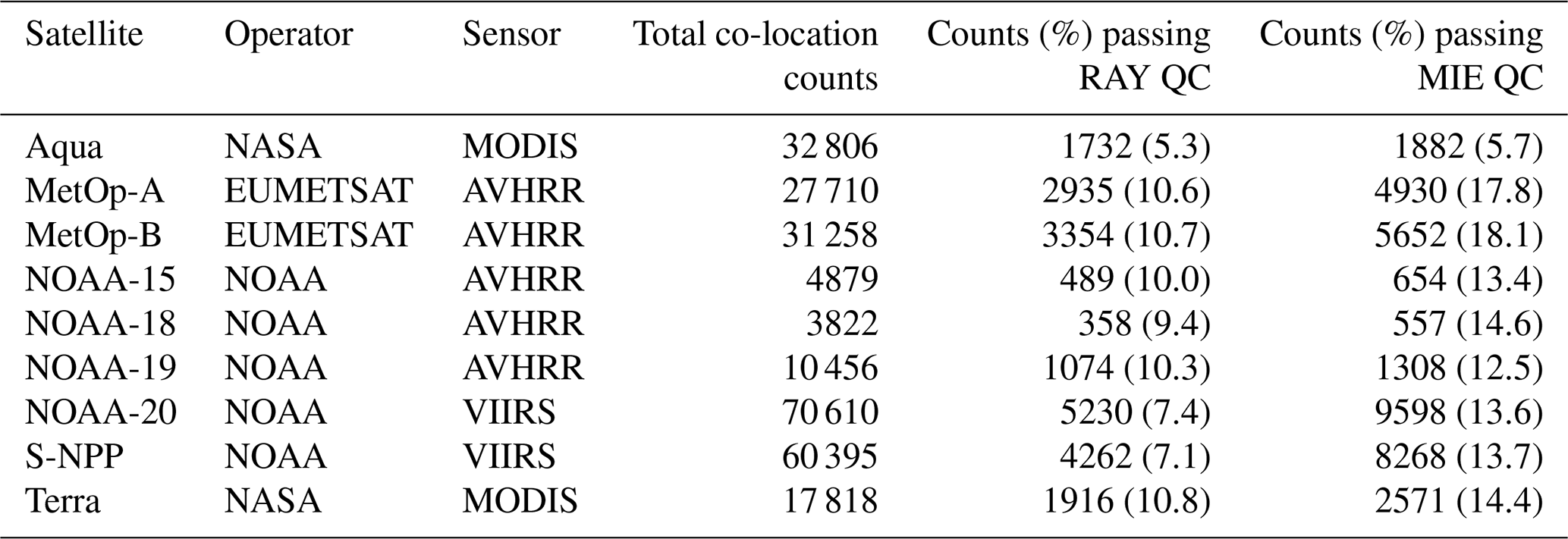
Table 1Co-location counts for each type of GEO AMV. The table lists total counts (RAY and MIE) and counts of co-located AMVs (percent of total in parentheses) with forecast-independent QI > 80 % that pass RAY QC and MIE QC.

Numerous studies have evaluated bias and uncertainty characteristics of AMVs through direct comparison with in situ rawinsonde observations and NWP analyses (e.g., Velden et al., 1997; Bormann et al., 2002, 2003; Le Marshall et al., 2008; Bedka et al., 2009; Velden and Bedka, 2009; Key et al., 2016; Daniels et al., 2018; Cotton et al., 2020). The derived motion wind algorithms that generate IR, WVcloud, and WVclear AMVs can vary between centers (Santek et al., 2014, 2019). AMV performance metrics vary significantly by season, level, type, satellite/producer, etc. (e.g., Santek et al., 2019; Daniels et al., 2018; Cotton et al., 2020; Key et al., 2016; Le Marshall et al., 2008). For example, typical values of AMV wind speed bias acquired from seven different data producers and verified against rawinsonde winds can range from −1.8 to 0.3 m s−1, and wind speed uncertainty represented by the standard deviation can range from 4 to 6.5 m s−1, with higher vector wind root mean square errors of 6–9 m s−1. Even for a single satellite, e.g., GOES-16 or Aqua, speed bias and uncertainty can vary geographically and vertically.
In fact, AMVs have state-dependent errors that can vary based on wind speed and water vapor content and gradient (Posselt et al., 2019). Past reports show that AMVs tend to exhibit a slow speed bias (1–5 m s−1) at high levels (above 400 hPa) in the extratropics and a fast speed bias (1–3 m s−1) at middle levels (400–700 hPa) in the tropics (Bormann et al., 2002; Schmetz et al., 1993; von Bremen, 2008). Recent improvements to AMV derivation schemes, e.g., in GOES-16/17 and Himawari-8, have reduced the fast speed bias, with the residual bias largely being attributed to height assignment errors (Cotton et al., 2020). Height assignments to the AMVs via satellite- and ground-based techniques (Jung et al., 2010; Salonen et al., 2015) have been shown to account for a large source of AMV uncertainty (Velden and Bedka, 2009). One factor of the height assignment error is that AMVs are generally assigned to discrete levels when, instead, they better correlate with atmospheric motions in layers of varying depth that depend on the vertical moisture profile (Velden et al., 2005; Velden and Bedka, 2009). Moreover, speed biases and uncertainties tend to be higher at higher elevations and in combination with strong wind shear (Bormann et al., 2002; Cordoba et al., 2017), and this is attributable to larger height assignment errors (hereafter the wind shear height assignment error effect).
Aeolus HLOS global wind profiles are co-located with satellite-derived AMVs. The co-location approach implemented here was also used by Hoffman et al. (2022) and follows that employed at the University of Wisconsin-Madison/Cooperative Institute for Meteorological Satellite Studies (CIMSS; Santek et al., 2021). AMV co-location datasets are prepared separately for RAY and MIE winds. (A single AMV might appear in both datasets.) AMV observations are compared with Aeolus observations from the same and neighboring 6 h cycles to account for all possible co-locations. An Aeolus observation is retained for comparison with an AMV if the Aeolus observation satisfies all of the following co-location criteria:
-
Aeolus time falls within 60 min of the AMV time.
-
Aeolus pressure is within 0.04 log10 (pressure) of the AMV height assignment. (Note that the log of pressures is used to account for the nonlinear decrease in pressure with increasing altitude.)
-
Aeolus observation location is within the 100 km horizontal great circle distance of the AMV location.
If multiple Aeolus observations satisfy these criteria for the same AMV observation, then the Aeolus observation closest in distance is retained. Then, if multiple Aeolus observations still meet all co-location criteria, the observation closest in pressure to the AMV observation is kept for analysis. There is no need to consider closeness in time, given the co-location criteria and the Aeolus orbit. After co-location, the AMV wind vector is projected onto the HLOS direction of its paired Aeolus observation.
Our choice of co-location criteria is conservative compared to those defined by the IWWG (International Winds Working Group) 1998 workshop (Velden and Holmlund, 1998). Although the larger time and distance criteria defined by IWWG (90 vs. 60 min and 150 vs. 100 km) might retain more co-location pairs and thus a larger sample, the co-located winds would more likely have larger MCDs and SDCDs. Our smaller time and distance criteria restrict the number of possible Aeolus matches to any one AMV and help avoid Aeolus matches from two different orbits. The IWWG height criterion is a fixed pressure difference (25 hPa) that might be too small at lower levels where pressure layers are tightly spaced in elevation but too large in the upper atmosphere where the elevation distance between pressure layers is much larger. Our height criterion is based on a log10 scale and accounts for the varying distances between pressure layers throughout the vertical and corresponds to pressure differences ranging from approximately 300 to 1 hPa for pressures from 1000 to 10 hPa, respectively.
Once co-located, Aeolus winds and AMVs are filtered by additional QC tests to retain pairs of QC'd observations. (QC was implemented after co-location in order to test and compare the use of different QC criteria without having to repeat the co-location process.) Aeolus QC criteria were chosen following the ESA's recommendations for the RAY and MIE observing modes, and these are consistent with those listed in Rennie and Isaksen (2020a). Specifically, RAY winds are rejected if winds are close to topography (pressure > 800 hPa), have horizontal accumulation lengths < 60 km, vertical accumulation lengths < 0.3 km, L2B uncertainty > 12 m s−1 at upper levels (pressure < 200 hPa), or L2B uncertainty > 8.5 m s−1 at lower levels (pressure > 200 hPa). L2B uncertainty refers to the Aeolus HLOS wind error estimate assigned to each wind measurement. Horizontal and vertical accumulation lengths refer to the horizontal and vertical distances over which individual measurement signals are accumulated and averaged to improve the signal-to-noise ratio. In this way, the Aeolus observations represent wind volumes and not discrete points or levels. The accumulation lengths can vary and depend on the processor settings. Similarly, MIE winds are rejected if winds are near topography (pressure > 800 hPa) or L2B uncertainty > 5 m s−1 at any level. For all AMVs, a forecast-independent quality indicator (QI) of at least 80 % is used to filter and retain the high-quality data; this threshold is recommended for AMV studies and in NWP by the user community and has been shown to improve statistical agreement between AMV-producing centers (Santek et al., 2019). No explicit outlier QC is applied, and since there are no extreme outliers (seen below in Figs. 6 and 9), the QC that is applied is sufficient to eliminate them. Total co-location counts per satellite and the percentage of observations that pass QC for each AMV type and Aeolus mode are presented in Tables 1–2. (It is noted that Himawari-8 and INSAT 3D WVclear AMVs are not included in the NCEP data archive.)
The performance of QC'd AMVs relative to co-located QC'd Aeolus winds are characterized by analyzing the statistics of the difference between AMV HLOSV minus Aeolus HLOSV. The two key statistics calculated for the co-location difference (always in the sense of AMV minus Aeolus) are the MCDs and the SDCDs. Because we are comparing the AMV and Aeolus HLOSV, a scalar quantity, our statistics can only be analogs of the standard one. We include the formulae for all the statistics in Appendix A. It is important to emphasize that the co-location differences have several components that include errors in both AMVs and Aeolus winds. Specifically, these are due to the observation error of the AMVs and Aeolus HLOSV, representativeness errors due to differences in scales observed, which are related to different shapes of the observing volumes, and to co-location errors due to the space and time mismatches between the observations. As previously mentioned, the estimated SD for Aeolus L2B winds is 3.8 m s−1 for MIE and 5.3 m s−1 for RAY. We note that it might be possible to estimate the statistics of the co-location and representativeness errors. The co-location difference may be considered to have the following three independent components: the error of the AMV winds, the error of the Aeolus winds, and the difference between the truth evaluated for the AMV and the Aeolus winds. We can isolate the first component, the AMV error, if we know the other two components, and we already have estimates of the second component, the Aeolus wind error in the L2B data. The last component is the error due to representativeness and co-location differences. The differences in time and location give rise to the co-location error. The difference in the shapes of the observing volumes gives rise to the representativeness error. If we simulate the AMV and Aeolus observations from a high-quality forecast or analysis or simulation, which is taken to be the truth, then we can calculate estimates of the combined representativeness and co-location errors. If the truth fields are simply interpolated to the observation locations, then the calculated estimates are for the co-location errors alone. For this study, we take the first step in isolating the co-location/representativeness errors by removing the influence of the Aeolus error from the SDCDs, as the simulation of the AMV and Aeolus observations is out of the scope of this study. The removal of the Aeolus error estimate results in a smaller SDCDs, which still includes AMV random and representativeness errors and the co-location error. The SDCDs are larger for RAY comparisons than for MIE comparisons in terms of both the original (or total) and adjusted values. Although the Aeolus L2B uncertainty is highly dependent on the time period and processor used to determine the HLOS winds, it is the correct uncertainty estimate for our study.

Figure 1Vertical comparisons of co-located GOES-16 AMVs and RAY winds in the tropics (30∘ S to 30∘ N). The top row shows Aeolus ascending orbits (ASCs), (a) mean AMV (solid lines), and RAY (dashed lines) winds (m s−1), (b) MCDs (solid), SDCDs (short dashed), and AMV HLOSV errors, as represented by the SDCD–Aeolus L2B uncertainty (long dashed; m s−1), and (c) co-location counts. Panels (d–f) are the same as panels (a–c) but for Aeolus descending orbits (DESCs). Colors denote the AMV type, with IR (red), WVcloud (blue), and WVclear (green). Colored open circles indicate levels where MCDs are statistically significant at the 95 % level (p value < 0.05), using the paired Student's t test. Vertical zero lines are displayed in the left and center panels in black. Levels with observation counts > 25 are plotted.
The geometry of the Aeolus observation affects how the HLOS winds are interpreted for analysis (Straume et al., 2018). The observed HLOSV provides both a speed and direction and represents the motion of air projected onto the line-of-sight of the laser that, in 2D space, is nearly orthogonal to the satellite orbit direction (see Fig. 5a in Lux et al., 2020). Thus, in the ascending orbit phase away from the poles, a positive HLOSV indicates a westerly wind, and a negative HLOSV indicates an easterly wind; the opposite is true for winds in the descending orbit phase. Figure 1 illustrates that, in the tropics, the HLOSV is approximately equal to the zonal wind in the ascending and descending orbit phases. In the left column of Fig. 1, profiles of mean HLOSV for AMVs (solid lines) and Aeolus (long dashed lines), as well as mean AMV wind speed not projected onto the HLOS direction (short dashed lines), are shown. In the center column of Fig. 1, HLOSV MCDs (solid lines) and total SDCDs (short dashed lines), as well as the adjusted SDCDs with the mean Aeolus L2B uncertainty removed (long dashed lines), are plotted. Open circles indicate pressure levels at which MCDs are statistically significant at the 95 % level (p value < 0.05), using the paired two-sided Student's t test. Corresponding co-location counts are shown in the right column of Fig. 1. The mean AMV and Aeolus HLOSV and their differences exhibit similar magnitudes of opposite sign throughout the vertical between the ascending (Fig. 1a–b) and descending (Fig. 1d–e) orbit phases. This indicates that mean HLOSV differences that include winds from both the ascending and descending orbit phases would be small and would represent differences of larger opposing magnitudes. Moreover, the removal of Aeolus L2B uncertainties from the total SDCDs results in adjusted SDCDs of similar magnitude between the orbit phases, implying that the quality of Aeolus winds is not wholly dependent on orbit phase during the study period. To simplify the interpretation of the observed HLOS winds, we multiply HLOSVs in descending orbit phases by −1. In doing so, a positive HLOSV (away from the poles) now indicates a westerly wind and negative a HLOSV an easterly wind, regardless of the Aeolus orbit phase. All statistics in what follows, including Figs. 2, 3, and 5–14, are based on co-location differences that combine ascending and −1 times for descending orbit phase winds.
In this section, we examine in detail the performance of AMVs from the GOES-16 GEO satellite and summarize the AMV performance of all LEO satellites available in the study period. Here, the reader should keep in mind that performance is relative to Aeolus and for the vector AMV projected onto the Aeolus HLOS. In agreement with previous studies, our results confirm that the level of agreement between AMVs and Aeolus winds varies per combination of conditions, including the observing scene type (clear vs. cloudy) coupled with AMV type, geographic region, and height of the observable. Moreover, the findings highlight the value of using Aeolus MIE winds as a comparison standard to characterize AMVs. For context, we begin with summary statistics for samples that include all conditions.
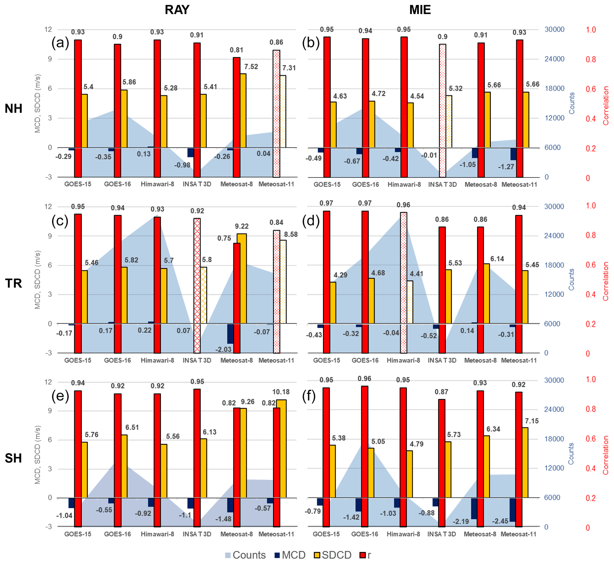
Figure 2AMV–Aeolus global mean statistics in the (a, b) NH, (c, d) tropics (TRs), and (e, f) SH for GEO satellites that include the correlation (r) in red, mean co-location difference (MCD) between the HLOS winds (AMV–Aeolus) in navy blue, standard deviation of the co-location difference (SDCD) in yellow, and co-location counts as light blue shaded areas. Solid colors denote the 95 % statistical significance, stripes denote the 90 % statistical significance, and dots indicate the differences that are not statistically significant.
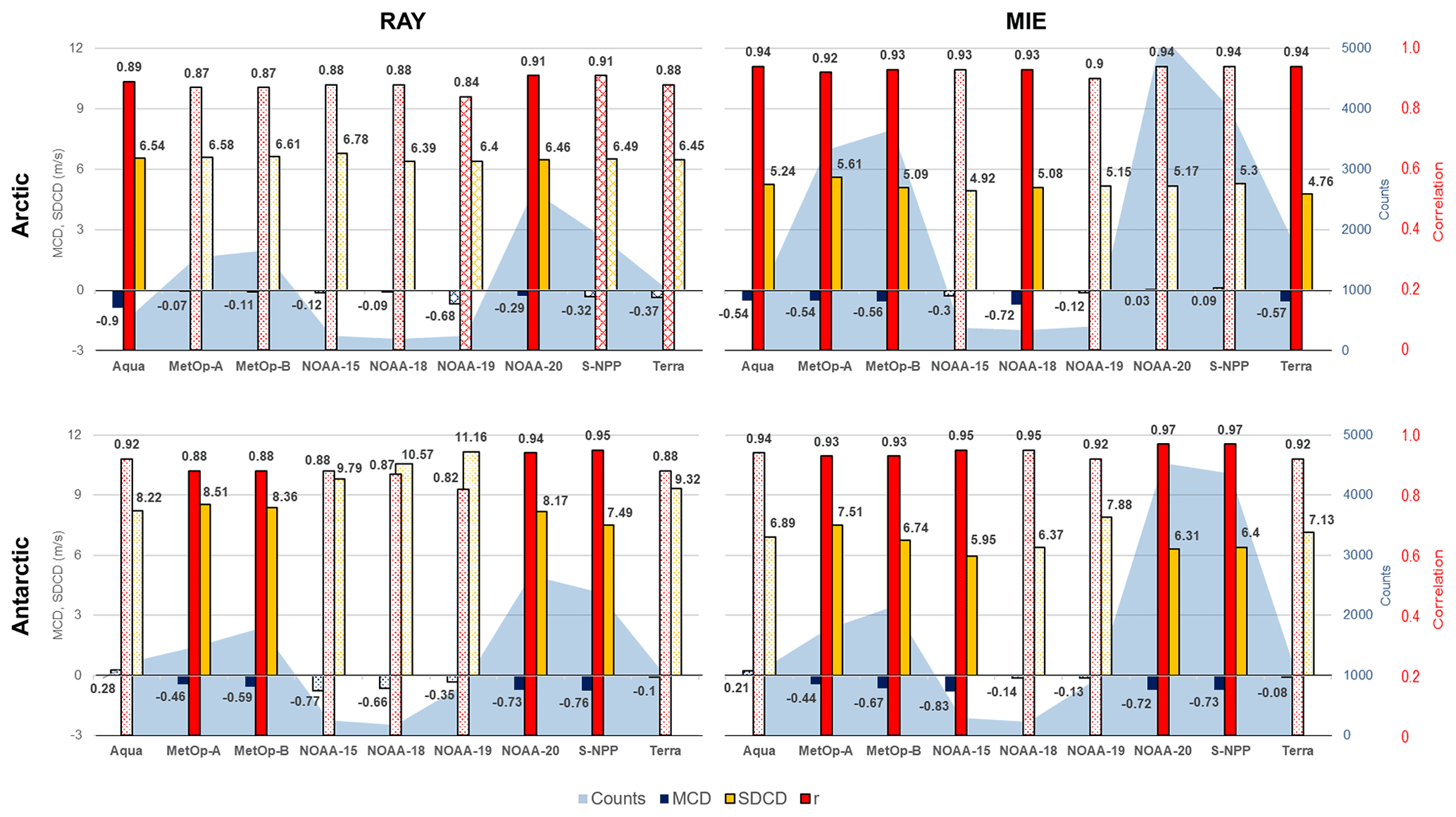
Figure 2 summarizes the performance of all available GEO AMV HLOS winds relative to Aeolus RAY (left column) and MIE winds (right column) in the period of study; likewise, Fig. 3 summarizes LEO AMV performance. The statistics include correlation (r), MCDs, and SDCDs, and their formulae are listed in Appendix A. The correlation between co-located HLOS winds describes the overall relation of AMVs to Aeolus. The other statistics have their usual meaning (Wilks, 2011) applied to the HLOSVs. Since the MCDs are small compared to the SDCDs, the RMSDs (root mean square differences) and SDCDs are very similar, and in the following we will only discuss the SDCDs, but any statement concerning the SDCDs also applies to the RMSDs. Using the paired two-tailed Student's t test, mean differences significantly different from zero at the 90 % (p value < 0.10) and 95 % (p value < 0.05) confidence levels are indicated in Figs. 2–3 by striped and solid bars, respectively, and dotted bars indicate the differences that are not statistically significant. Observation counts are displayed by gray-blue shading. Direct comparisons between our statistics and those from previous studies are limited because all our statistics are HLOSVs and not vector winds. Although we compare mean AMV–Aeolus co-location differences with speed statistics, recall that, in general, the HLOS wind generally approximates the zonal component of the horizontal flow rather than the wind speed.
The main points from the summary co-location statistics of RAY and MIE winds with AMVs are the following: MIE comparisons exhibit higher correlations and lower SDCD values relative to RAY, thereby reflecting the general higher accuracy of MIE vs. RAY winds. In Fig. 2, GOES and Himawari-8 AMVs have high correlations with Aeolus (> 0.90). MCDs vary, depending on the AMV satellite, but are generally smallest in the tropics and largest in the SH extratropics where the SDCDs are larger. For RAY comparisons with GOES and Himawari-8 AMVs, the SDCDs range from 5.27 m s−1 in the NH extratropics to 6.5 m s−1 in the SH extratropics and are comparable to wind speed RMSDs relative to rawinsonde winds (Santek et al., 2019). Of the satellites listed in Fig. 2, Meteosat wind correlations are lowest, and the corresponding SDCD values are highest by at least 2–3 m s−1. LEO AMV–Aeolus co-locations in Fig. 3 exhibit statistically significant MCDs that are comparable to observed wind speed biases for Aqua and Terra AMVs (Key et al., 2016; Le Marshall et al., 2008). AMVs from most LEO satellites exhibit higher SDCD values by ∼ 1–2 m s−1 relative to GEO, particularly in the Antarctic, where SDCD values are of the order of 7.5–8.5 m s−1 for RAY and 5.9–7.5 m s−1 for MIE.
Differences in the SH extratropics and Antarctic pole exhibit higher SDCD values compared with the rest of the globe. This is likely due to several factors. During the study period, the SH region of GEO fields of view covers a portion of the winter storm tracks that propagate eastward all the way around the Southern Ocean. The SH storm tracks exist year-round, and in winter (June–July–August) the upper-tropospheric subtropical jet is stronger and acts as a waveguide for eastward-propagating baroclinic waves over a broader latitude range (Trenberth, 1991; Nakamura and Shimpo, 2004; Hoskins and Hodges, 2005), thus amplifying wind shear and storm track intensity. This is one factor that explains the higher SDCD values observed in GEO differences in the SH extratropics, as AMV uncertainties tend to increase with increasing wind speed (Posselt et al., 2019) and high wind shear (Bormann et al., 2002; Cordoba et al., 2017). In the Antarctic polar region, the general strengthening of the polar vortex aloft in late winter/early spring (i.e., during the study period) is related to a stronger Equator-to-pole temperature gradient brought about by gradually increasing subtropical lower stratospheric temperatures from March to September (Zuev and Savelieva, 2019). A stronger Antarctic polar vortex is associated with stronger zonal winds aloft (and stronger shear), which could increase the corresponding SDCD values for AMVs due to the wind shear height assignment error effect. Surface effects may also play a role, as very cold brightness temperatures at or near the polar surface may be misinterpreted as cloud tops due to the low temperature contrast between clouds and the surface snow or ice (Key et al., 2016).
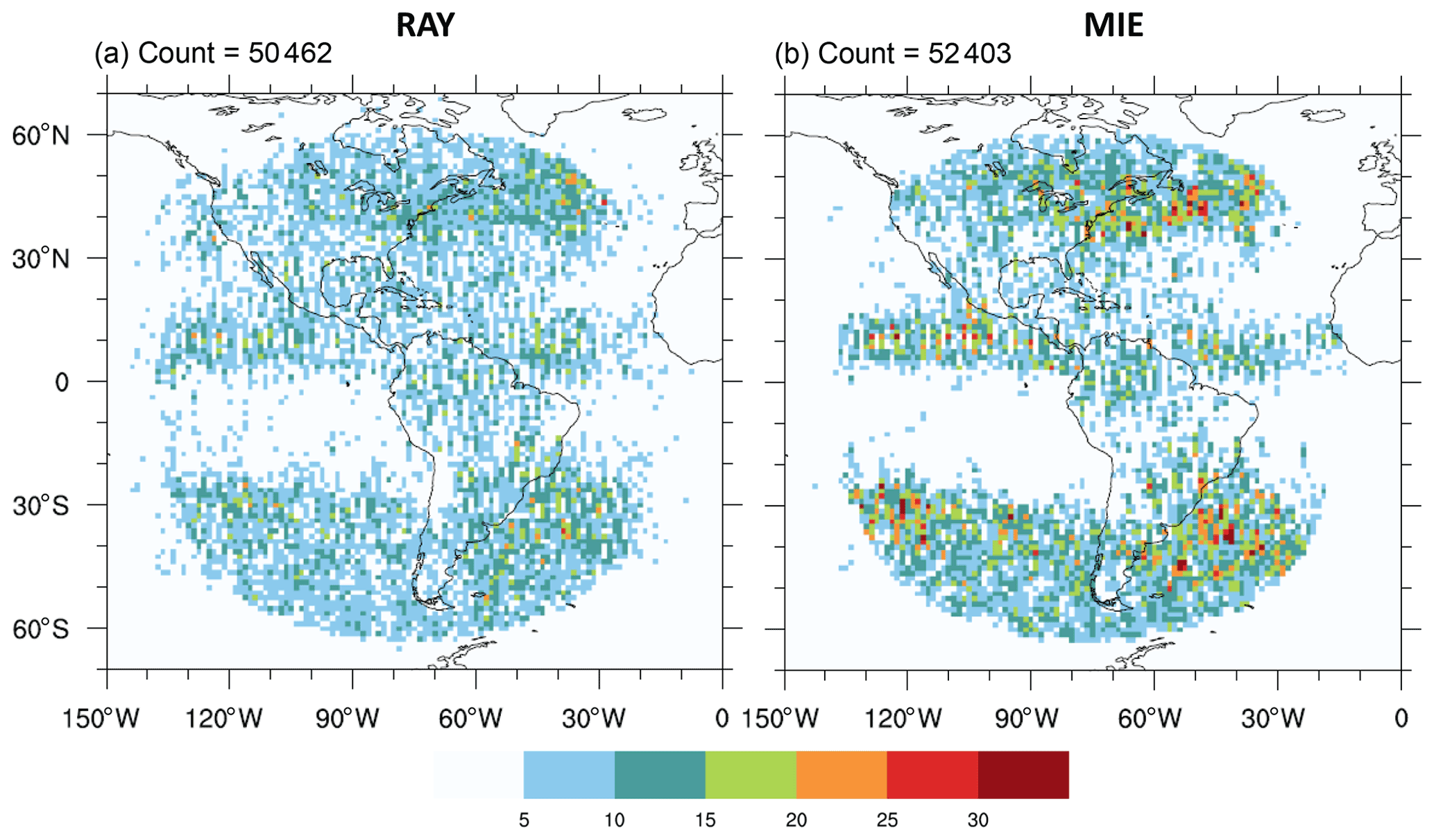
Figure 4Number densities of quality-controlled GOES-16 AMV observations co-located with quality-controlled Aeolus (a) Rayleigh-clear (RAY) and (b) Mie-cloudy (MIE) HLOS winds. Colors indicate total number of co-located observation pairs within a grid cell at 1.25∘ (approximately 140 km in the N–S direction) horizontal resolution. Total observation count per panel is displayed at the top left corner. This and all subsequent plots are for all co-locations with quality-controlled AMV and Aeolus winds during the study period (2 August to 16 September 2019).
As a case study, we examine in greater detail the performance of AMVs from GOES-16, a GEO satellite (Sect. 4.1). This is done because, compared with other GEO satellites, GOES-16 exhibits high correlations with Aeolus RAY (> 0.90) and MIE winds (> 0.94), relatively small SDCDs (5.8–6.5 m s−1 for RAY and 4.7–5 m s−1 for MIE), and have the largest extratropical sample size from which to compute robust statistics (see Fig. 2). The other GEO satellites are not further examined as they exhibit larger RAY SDCDs (Meteosat-8 and Meteosat-11), have a much smaller extratropical sample size (Himawari-8, Meteosat-8, and Meteosat-11), or are not actively used in NCEP operations (GOES-15 and INSAT-3D). GOES-16 AMVs are derived from full disk images centered at 75.2∘ W longitude from the onboard Advanced Baseline Imager (ABI). GOES-16 cloud-top AMVs are generally of good quality and, when validated against rawinsonde winds, exhibit a relatively small mean difference in wind speed ranging from −1.0 to +0.5 m s−1 and mean vector differences of 3–6 m s−1 that tend to increase with height (Daniels et al., 2018). Figure 4 presents the GOES-16/Aeolus co-location number densities (i.e., the total number of co-located observation pairs within each grid cell on a 1.25∘ (∼ 140 km) resolution map) covering the period of study. QC'd GOES-16 AMVs co-located with QC'd RAY and MIE winds are shown in Fig. 4a and b, respectively. MIE co-locations exhibit three bands of high-density winds along the Intertropical Convergence Zone (ITCZ) and extratropical storm tracks, with few winds found between 0–30∘ S. A similar but smoother version of the MIE distributions is shown for co-located RAY winds. The MIE co-location number density is greater than that for RAY, as AMV observation density tends to be higher in very cloudy or very moist scenes (Velden et al., 1997).
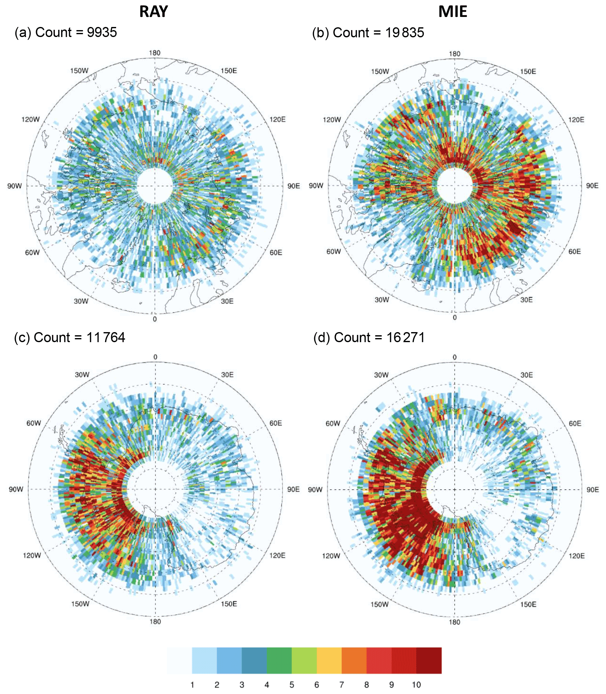
Figure 5Number densities of IR-derived AMVs from all available LEO satellites co-located with Aeolus RAY (a, c) and MIE (b, d) winds in the (a, b) Arctic (north of 60∘ N) and (c, d) Antarctic (south of 60∘ S) are shown. Colors indicate total number of co-located observation pairs within a grid cell at 1.25∘ (approximately 140 km in the N–S direction) horizontal resolution. Dashed latitude lines are spaced every 5∘. The total observation count per panel is displayed in the top left corner.
For the LEO perspective, we choose to examine the performance of all LEO IR AMVs rather than from a single satellite (Sect. 4.2). This is done because, compared to GEO, LEO AMVs from each satellite comprise a relatively small sample of co-located winds, and this would render any associated performance metric unreliable. Furthermore, unlike the suite of available GEO satellites, where each observe a different region of the globe (except for small areas where the footprints of neighboring satellites overlap), each LEO satellite observes AMVs in the same polar regions and thus samples the same atmospheric motions. Figure 5 depicts the observation number densities of QC'd LEO AMVs co-located with QC'd RAY and MIE winds in the Arctic and Antarctic polar regions bounded by 60∘ latitude for Arctic RAY (Fig. 5a), Arctic MIE (Fig. 5b), Antarctic RAY (Fig. 5c), and Antarctic MIE (Fig. 5d). In general, more LEO/MIE co-location pairs pass QC and are retained in the analysis than for RAY winds. Co-locations in the Arctic are found across the high latitudes, with MIE comparisons exhibiting higher concentrations poleward of Eurasia and North America. Antarctic co-locations are primarily found over the western half of the continent. In this region, water vapor features are more suitable for tracking and deriving AMVs as they exist downstream of intense upper-level storm tracks (Hoskins and Hodges, 2005) in an area of higher annual precipitation (Grieger et al., 2016).
4.1 GOES-16 AMVs vs. Aeolus
To increase the size of our co-location dataset, we compared all types of GOES-16 AMVs to both Rayleigh-clear and Mie-cloudy winds. In addition, we do not show results from WVclear AMV co-locations with Mie-cloudy winds, as correlations for this category of co-locations are poor, and the sample size is very small (see Table 1), and this result may be unreliable. With a larger dataset, it might be possible to compare Rayleigh-clear and Mie-cloudy winds to clear and cloudy AMVs only, respectively. Additionally, winds retrieved from tracking clear-sky and cloud motions represent different dynamical features and tend to behave differently. For example, the recommended time interval for tracking cloud motions is 10–15 min to capture short cloud lifetimes and rapid intensification/deformation, while the recommended time interval for clear-air motions of 30 min is suitable to capture variations in jet streams and other clear-air features (Schmetz et al., 2000).
4.1.1 Rayleigh-clear (RAY) comparisons
Figure 6 depicts density scatterplots that summarize the relationship of GOES-16 AMVs to RAY winds to highlight the regional differences in IR (Fig. 6a, d, g), WVcloud (Fig. 6b, e, h), and WVclear AMVs (Fig. 6c, f, i). Sample statistics are based on Aeolus as the reference dataset and are displayed in the lower right of each panel. AMVs are highly correlated with RAY winds (0.88–0.91 in the extratropics and 0.93–0.95 in the tropics), with most co-locations for each AMV type falling close to the one-to-one line that indicates a perfect match. Note that, in the NH and SH extratropics, most co-locations are found in the upper-right quadrant, where HLOS winds are of positive sign and indicate the dominant westerly flow of the extratropics. In the tropics, many co-locations are grouped in the lower-left quadrant that indicates the easterly flow of the tropical trade winds at lower levels, and the rest are found in the upper-right quadrant that represents westerly tropical flow at upper levels. Of the three AMV types, the best match is for WVclear AMVs, with the comparisons exhibiting the smallest SDCD values in each geographic region that, in turn, are comparable to known wind speed SD and RMS (root mean square) of all GEO AMVs relative to rawinsonde winds (Santek et al., 2019). This is expected since WVclear AMVs and Aeolus RAY winds are most probably sampling similar clear-sky scenes, and clear scenes are more homogeneous over time and space scales, which, in turn, implies smaller co-location differences. Ideally, one would expect samples large enough to provide statistically significant co-location differences between RAY winds and WVclear AMVs only; as it turns out, the co-location differences are also statistically significant for IR and WVcloud AMVs (see Fig. 7). In these cases, cloudy AMVs are co-located with Aeolus RAY winds that represent clear scenes, and since they do not observe the same type of scene, Aeolus and/or AMV representativeness errors are most probably larger (hereafter we refer to this as the cloudy/clear sampling effect).

Figure 6Density scatterplots of co-located GOES-16 AMVs and RAY winds. Rows are for the (a–c) NH extratropics (30–60∘ N), (d–f) tropics (TRs; 30∘ S to 30∘ N), and (g–i) SH extratropics (30–60∘ S). Columns are for different AMV types, including (a, d, g) IR, (b, e, h) WVcloud, and (c, f, i) WVclear. Colors indicate total number of co-located observation pairs within the cells plotted, which are 1 m s−1 on a side. Sample statistics are displayed in the bottom right corner of each panel. Horizontal and vertical zero lines are plotted in black, as is the diagonal one-to-one line. The red star denotes statistical significance at 95 %, using the paired two-tailed Student's t test. HLOSV units are in meters per second (hereafter m s−1).
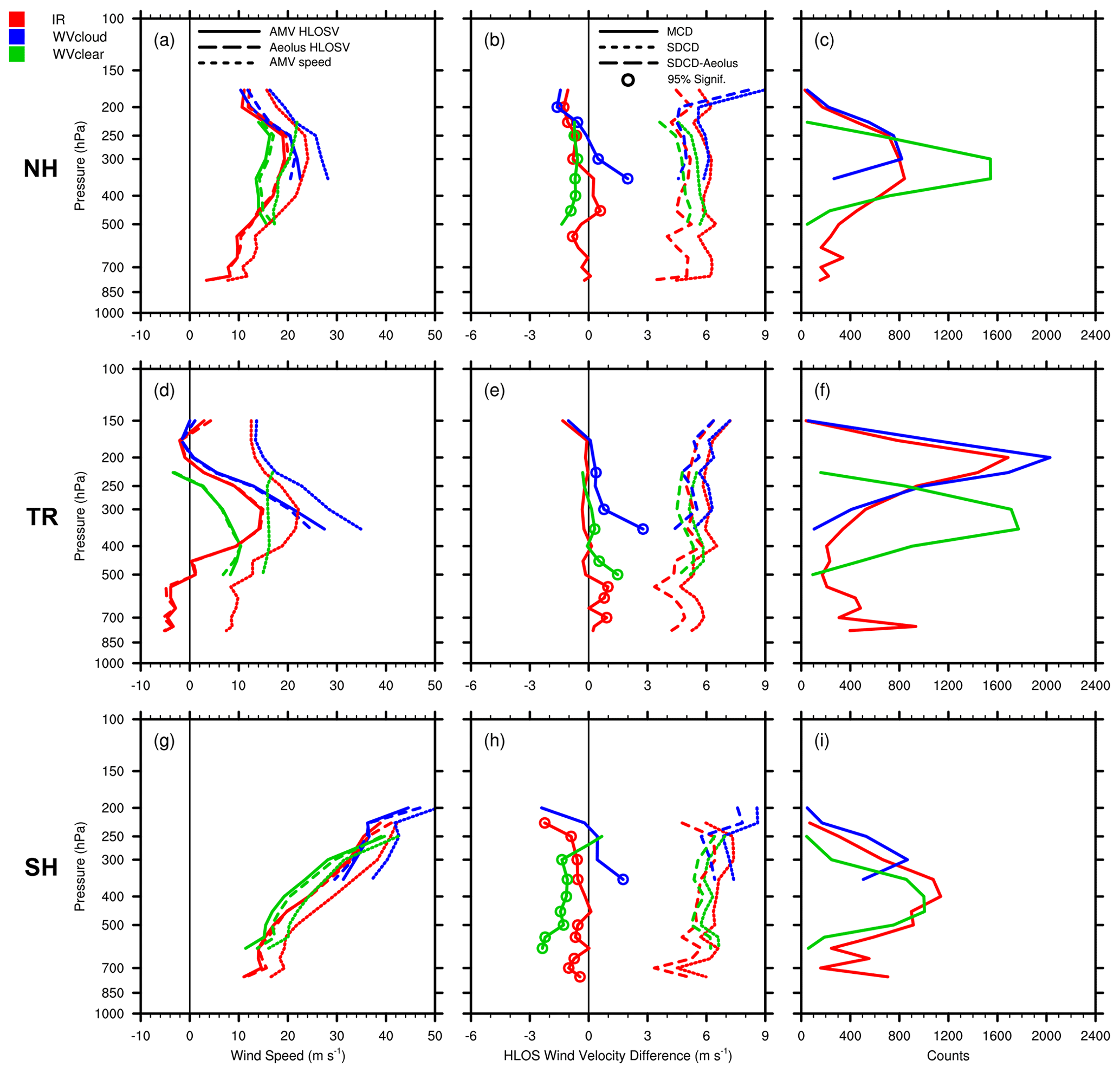
Figure 7Vertical profiles of co-located GOES-16 AMVs and RAY winds. The top row shows the NH extratropics (30–60∘ N), (a) mean AMV HLOSV (solid lines), RAY HLOSV (long dashed lines), mean AMV wind speed (short dashed lines; m s−1), (b) MCDs (solid), SDCDs (short dashed) and AMV HLOSV errors, as represented by SDCD–Aeolus L2B uncertainty (long dashed; m s−1), and (c) co-location counts. Panels (d–f) are as in panels (a–c) but for the tropics (30∘ S to 30∘ N), and panels (g–i) are as in panels (a–c) but for the SH extratropics (30–60∘ S). Colors denote the AMV type, including IR (red), WVcloud (blue), and WVclear (green). Colored open circles indicate levels where MCDs are statistically significant at the 95 % level (p value < 0.05), using the paired Student's t test. Vertical zero lines are displayed in the left and center panels in black. Levels with observation counts > 25 are plotted.
Figure 7 presents mean vertical profiles of GOES-16 AMVs and Aeolus RAY winds and corresponding MCD and SDCD distributions, similar to what is shown in Fig. 1. This perspective can provide additional insight into the accuracy of AMVs in representing the mean horizontal flow throughout the atmospheric column. Mean vertical profiles are plotted per AMV type in the NH extratropics (Fig. 7a–c), tropics (Fig. 7d–f), and SH extratropics (Fig. 7g–i). In Fig. 7a, d, and g, AMV HLOSV (solid lines) and Aeolus HLOSV (long dashed lines) generally show good agreement at all latitudes, and large gradients of HLOSVs correspond to layers of strong vertical wind shear inferred by the higher rate of change of AMV wind speed in the vertical (short dashed lines). Corresponding MCDs are statistically significant at most levels at all latitudes (Fig. 7b, e, and h) and seem to depict known AMV biases relative to high-quality sources of wind profile observations, particularly outside of the SH. For example, in the NH extratropics, MCDs range from −0.5 to −1.0 m s−1 at levels where co-location counts peak and could represent a small slow AMV bias, as previously noted by Bormann et al. (2002). In the tropics, AMVs exhibit an apparent small fast bias, which is the positive MCDs of 0.5 to 1.0 m s−1 that could be associated with larger AMV errors (and larger Aeolus errors) in layers of high winds and strong vertical wind shear (Cotton et al., 2020).
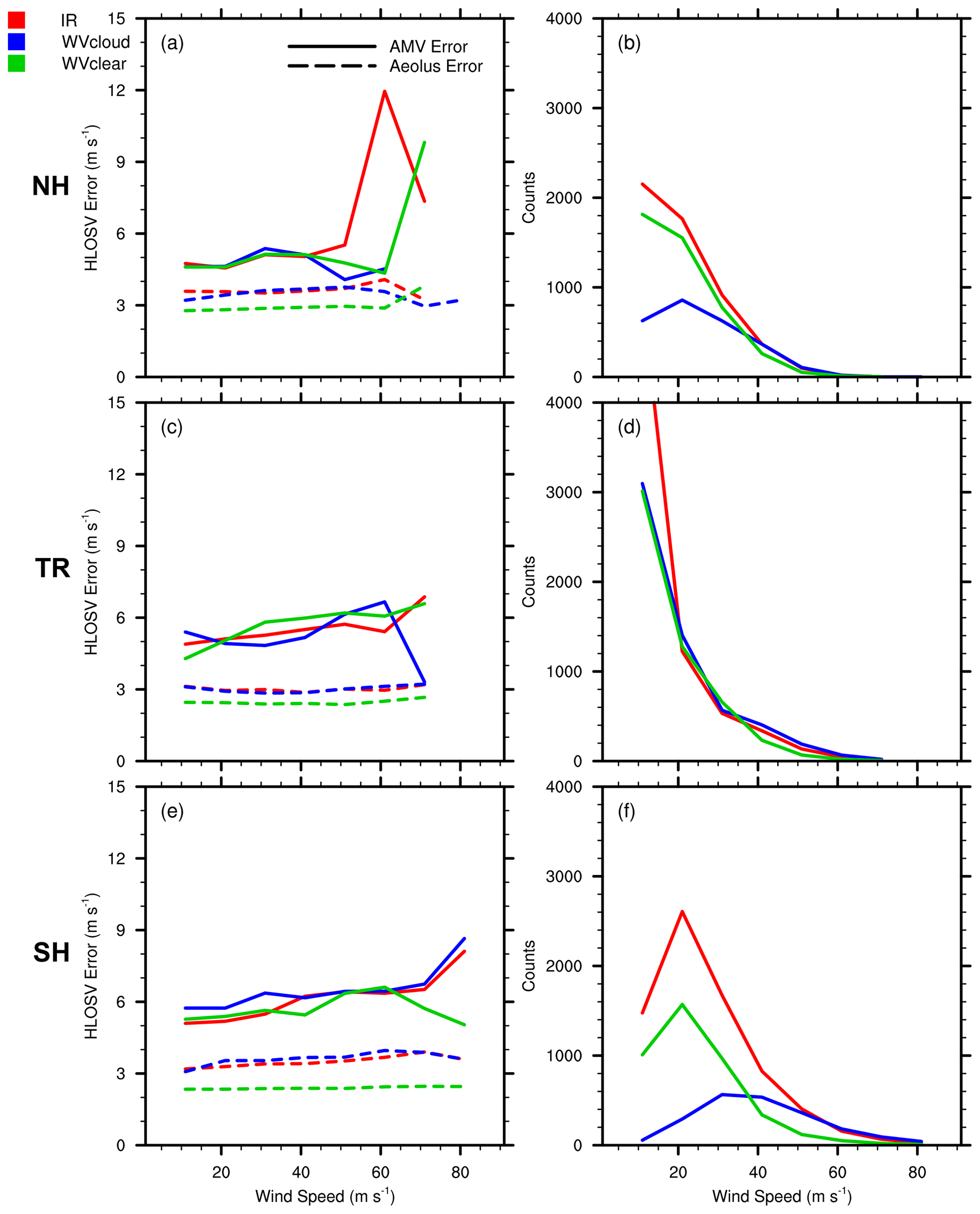
Figure 8AMV HLOSV error (SDCD–Aeolus uncertainty) derived from GOES-16 RAY comparisons (solid lines; m s−1) and Aeolus L2B uncertainty (dashed lines; m s−1) with respect to AMV wind speed binned at 10 m s−1 for (a) NH, (c) tropics (TRs), and (e) SH. (b, d, f) Counts per 10 m s−1 bin for each region.
Profiles of the total RAY SDCDs (short dashed lines in Fig. 7b, e, and h) that include AMV errors, Aeolus errors, and co-location/representativeness errors exhibit rather large values (> 6 m s−1) that tend to increase with height in layers of strong wind shear, particularly in the tropics, and SH extratropics. Moreover, the Aeolus QC acts to retain HLOSVs with larger uncertainties at levels above 200 hPa; this would explain the corresponding increase in total SDCDs at those levels. To better isolate the AMV error, the Aeolus error estimate is removed from the total SDCDs at each level, resulting in mean profiles of adjusted SDCDs (long dashed lines in Fig. 7b, e, and h) that include AMV errors and co-location/representativeness errors. Overall, the adjusted SDCDs for all AMV types exhibit similar magnitudes and distributions in each geographic region throughout the vertical. WVclear comparisons have slightly smaller adjusted SDCDs at the upper levels, suggesting that sampling differences may play a role in the higher accuracy observed for WVclear AMVs, given that WVclear representativeness errors are likely small due to Aeolus RAY and WVclear AMVs observing similar scenes. Aeolus RAY uncertainty is larger in the presence of clouds and appears to have a considerable impact on the corresponding SDCDs, as the reductions in IR and WVcloud SDCDs (∼ 1 m s−1) are larger than for WVclear SDCDs (0.5 m s−1). In the NH extratropics, the adjusted SDCDs for each AMV type is generally constant around 5 m s−1, and in the tropics it increases with decreasing pressure from 5 to 6 m s−1. AMV–RAY comparisons generally exhibit larger MCDs and SDCDs in the SH extratropics at upper levels due to the wind shear height assignment error effect. This is illustrated in Fig. 8, which shows that the adjusted SDCDs (solid lines) for all AMV types notably increase with increasing AMV wind speed in the SH extratropics relative to the other regions. This is also true for Aeolus error estimates (dashed lines) associated with IR and WVcloud comparisons in the SH (Fig. 8e).
4.1.2 Mie-cloudy (MIE) comparisons
Figure 9 presents density scatterplots like those in Fig. 6 but compares GOES-16 AMVs and MIE winds. MIE SDCDs are considerably smaller than those for RAY comparisons, and this is attributed to the general higher accuracy of Aeolus MIE wind retrievals. Another possible reason is that MIE comparisons might generally have smaller co-location errors. Because co-located Aeolus MIE winds and IR and WVcloud AMVs are, by definition, more likely sampling similar cloudy scenes at similar altitudes, we expect the Aeolus and AMV random and representativeness errors to be small (hereafter the cloudy/cloudy sampling effect). IR and WVcloud AMVs are highly correlated with MIE winds, ranging from 0.93 in the NH extratropics to 0.97 in the tropics. Most MIE co-locations fall along the one-to-one line that corresponds to a perfect match. Statistics of AMV minus MIE co-location differences are generally consistent, albeit with some notable exceptions, with those for AMV comparisons with high-quality rawinsonde winds. MCDs and SDCDs are smallest in the tropics at −0.3 and 4.4 to 4.6 m s−1, respectively, particularly for WVcloud comparisons, which seem to have the fewest outliers. SH extratropical comparisons exhibit the largest SDCDs (around 5 m s−1) but are still comparable to those associated with high-quality rawinsonde winds (Velden and Bedka, 2009; Santek et al., 2019). The smaller SDCDs observed in the NH and tropics suggest that AMVs accurately represent cloud-tracked motions associated with the North Atlantic storm track in summer and the summer-shifted ITCZ; such features are well defined by high MIE number densities in the north and middle portions of the GOES-16 field of view in Fig. 4b. The larger SH SDCDs suggest reduced accuracy in AMV winds that could be due to the wind shear height assignment error effect.
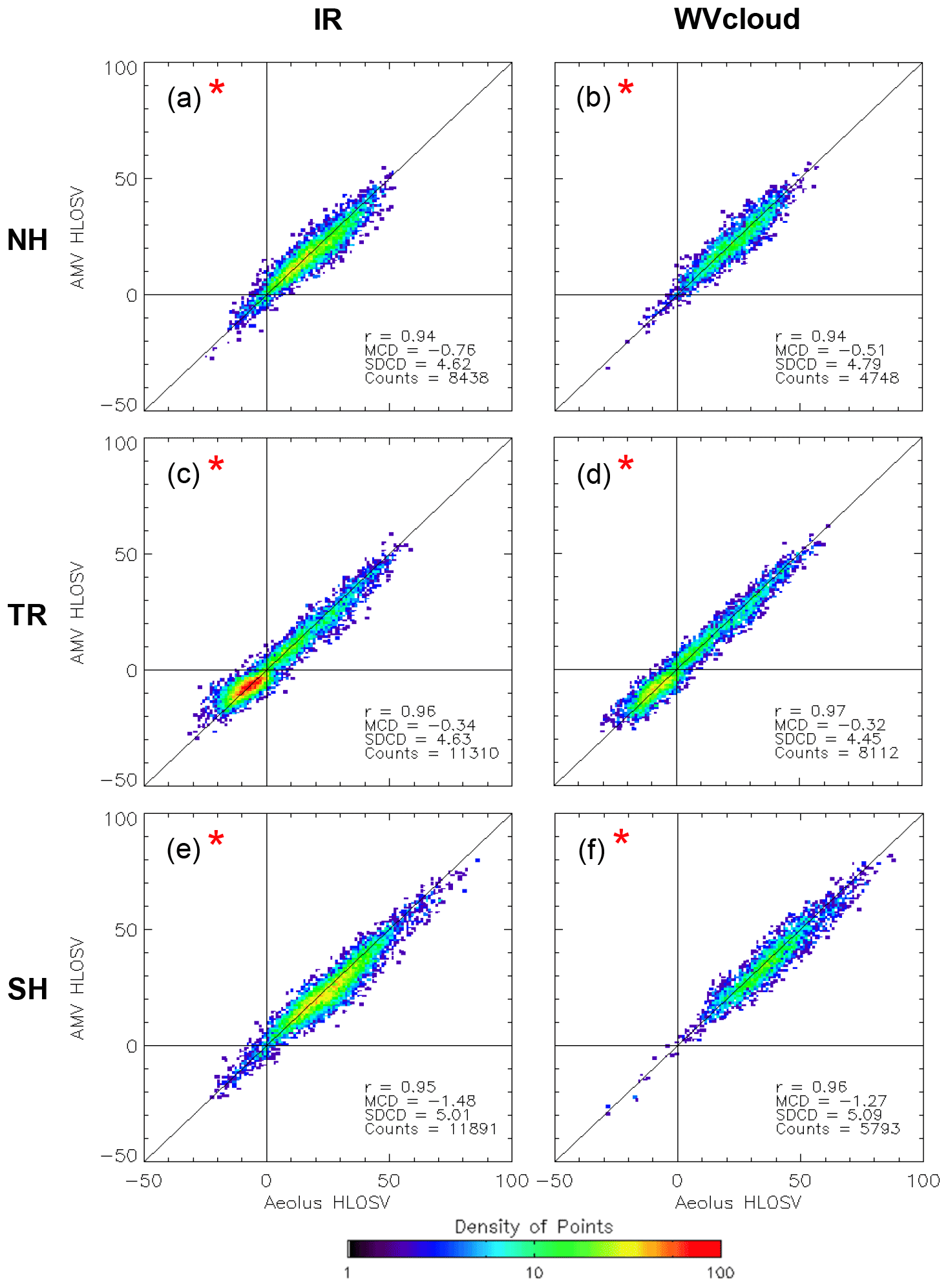
Figure 9As in Fig. 6 but for comparisons of IR (a, c, e) and WVcloud (b, d, f) AMVs and MIE winds.
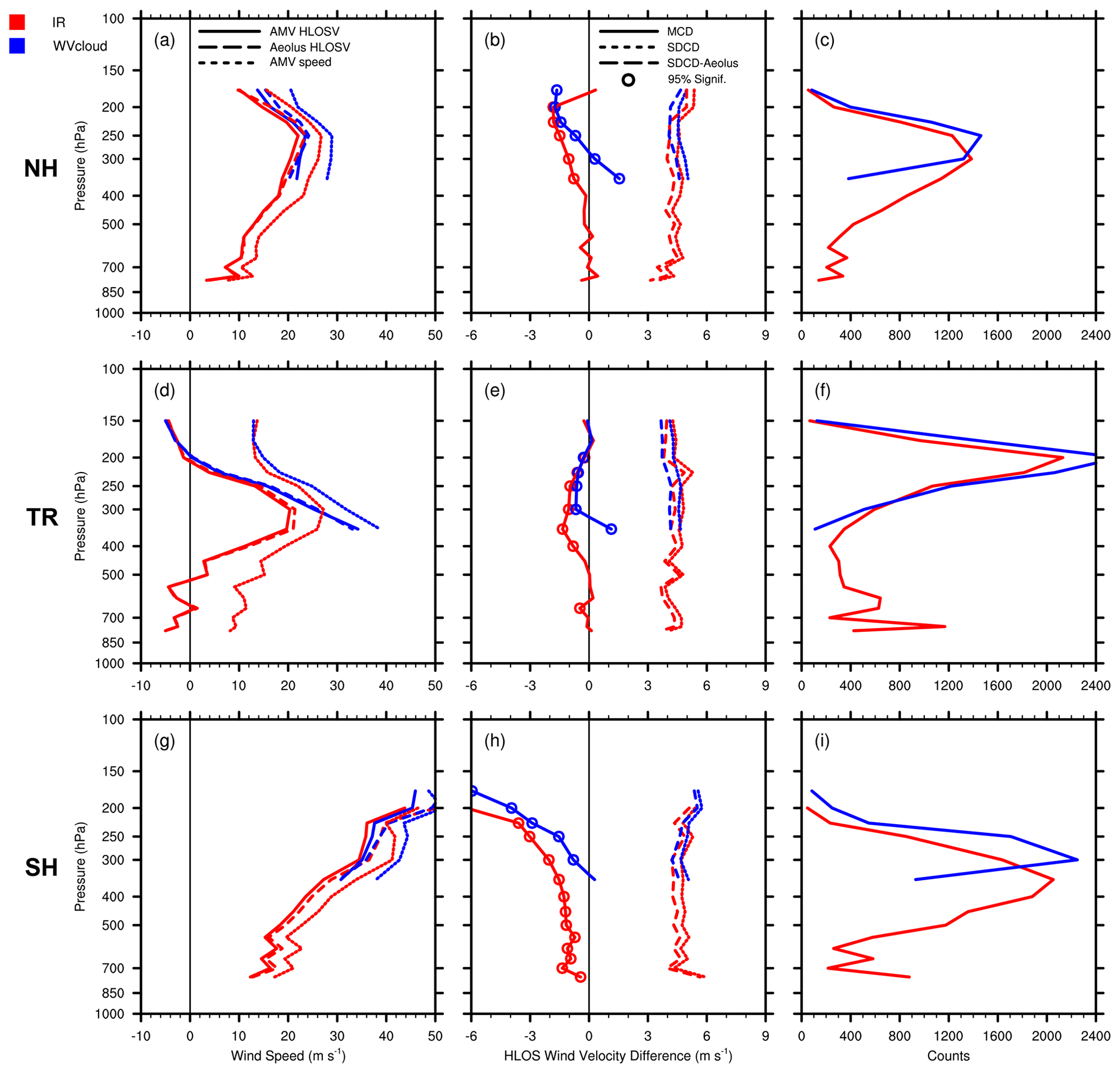
Figure 10As in Fig. 7 but for comparisons of IR (red) and WVcloud (blue) AMVs and MIE winds.
Similar to Fig. 7, Fig. 10 depicts vertical distributions of AMV and MIE HLOSVs and their differences. In the tropics and NH extratropics, MIE comparisons have nearly identical profiles of HLOSVs for the IR and WVcloud samples, with the largest MCDs observed at mid-levels in the tropics (at −1.5 m s−1) and at upper-levels in the NH extratropics (−2.0 m s−1), respectively. However, some of the larger differences occur at levels with a small sample size and may not be reliable. Despite the vertical variation in the MCDs, profiles of total and adjusted SDCDs are relatively constant at 4–5 m s−1, and the contribution of Aeolus uncertainty to the total SDCDs is small, as the removal of Aeolus errors only slightly reduces the SDCDs. The results suggest that, for MIE comparisons, the dominant factors contributing to the error consist of some combination of AMV random and representativeness/co-location error.
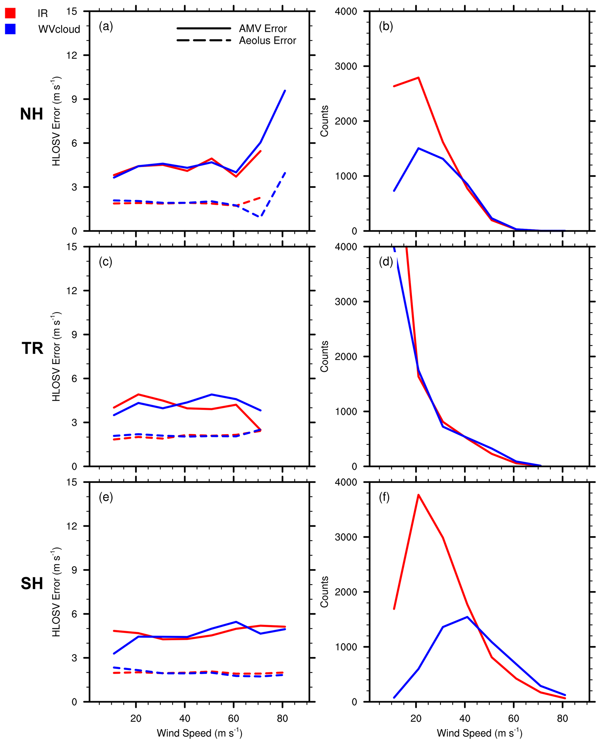
Figure 11As in Fig. 8 but for MIE comparisons with GOES-16 IR (red) and WVcloud (blue) AMVs.
In the NH above 250 hPa, SDCDs increase slightly with decreasing pressure in a region of strong wind shear that could lead to larger AMV height assignment errors and representativeness errors. Indeed, the adjusted SDCD is shown to be larger for faster AMV wind speeds while the corresponding Aeolus MIE error estimates remain relatively constant (Fig. 11). This result, in combination with likely small AMV-MIE co-location errors from the cloudy/cloudy sampling effect, suggests that AMV height assignment errors dominate the larger SDCDs observed in layers of high wind speed and strong shear. Additionally, in the tropics, a comparison with Aeolus MIE winds reveals a negative HLOSV bias in the IR and WVcloud GOES-16 AMVs below the higher cloud tops of the ITCZ (Fig. 10e). Larger MCDs appear at levels with higher wind speeds, as do larger values of adjusted SDCDs, although the samples are small. Because Aeolus MIE errors remain small and constant around 2 m s−1, with respect to AMV wind speed (Fig. 11c), and AMV-MIE co-location errors are likely small, the results suggest that AMV height assignment errors contribute most to the negative MCDs and corresponding larger SDCDs, in agreement with Cotton et al. (2020, 2021), who also note a negative bias largely thought to be attributed to AMV height assignment errors. This finding is relatively new, and the fact that comparisons with Aeolus depict this feature hints at the value of using Aeolus MIE winds as a standard for comparison to characterize cloud-tracked AMVs. Additionally, our comparisons with Aeolus depict another noted feature in monitoring AMVs by Cotton et al. (2020, 2021): a pronounced negative wind speed bias in the tropics for Meteosat-8 is evidenced by large negative MCDs and corresponds to large SDCDs in all regions (not shown). This feature is evident in both RAY and MIE comparisons.
MCDs are largest in the SH extratropics and are statistically significant throughout the vertical, ranging from −1.0 m s−1 at low levels to < −3.0 m s−1 above 300 hPa (Fig. 10h). Strong wind shear corresponding to an intensified jet is inferred at upper levels (Fig. 10g). The larger MCDs aloft are associated with increases in adjusted SDCDs with height, which are of the order of 4–6 m s−1. Moreover, the large MCDs represent over 8.5 % of the corresponding HLOSVs at upper levels and could be attributed to larger AMV height assignment errors corresponding to stronger storm tracks in winter. This is exemplified in Fig. 11e, where Aeolus MIE errors are shown to be small (2 m s−1) and remain relatively constant with increasing AMV wind speed, while the adjusted SDCDs are larger and increase with AMV wind speeds > 40 m s−1. The results imply that the large systematic differences in MCDs at upper levels in the SH extratropics are most probably attributed to larger AMV errors in combination with strong wind shear.
4.2 LEO AMVs vs. Aeolus
Figure 12 presents density scatterplots that compare LEO AMVs derived from IR window channels with RAY and MIE winds in the Arctic (Fig. 12a–b) and Antarctic (Fig. 12c–d) during the study period. LEO AMVs show good correspondence with both Aeolus observing modes in the polar regions. In general, comparisons in the Arctic have small yet significant MCDs (around −0.2 m s−1) and SDCDs estimates of 5.2–6.5 m s−1, while Antarctic comparisons exhibit larger MCDs and SDCDs. Moreover, MIE comparisons in the Arctic exhibit the smallest SDCDs, and RAY comparisons in the Antarctic have the largest SDCDs and more evident outliers. This suggests that, during the study period, IR LEO AMVs are best able to capture cloud-tracked motions during the summer season (in the Arctic) when cloudiness increases in the vertical and more water vapor content is generally available to track features (Alekseev et al., 2018). Water vapor content in the Arctic is largest in summer due to an influx of water vapor from melting ice and snow and receding sea ice extent, as well as intensified meridional moisture fluxes from low latitudes (Alexseev et al., 2018).
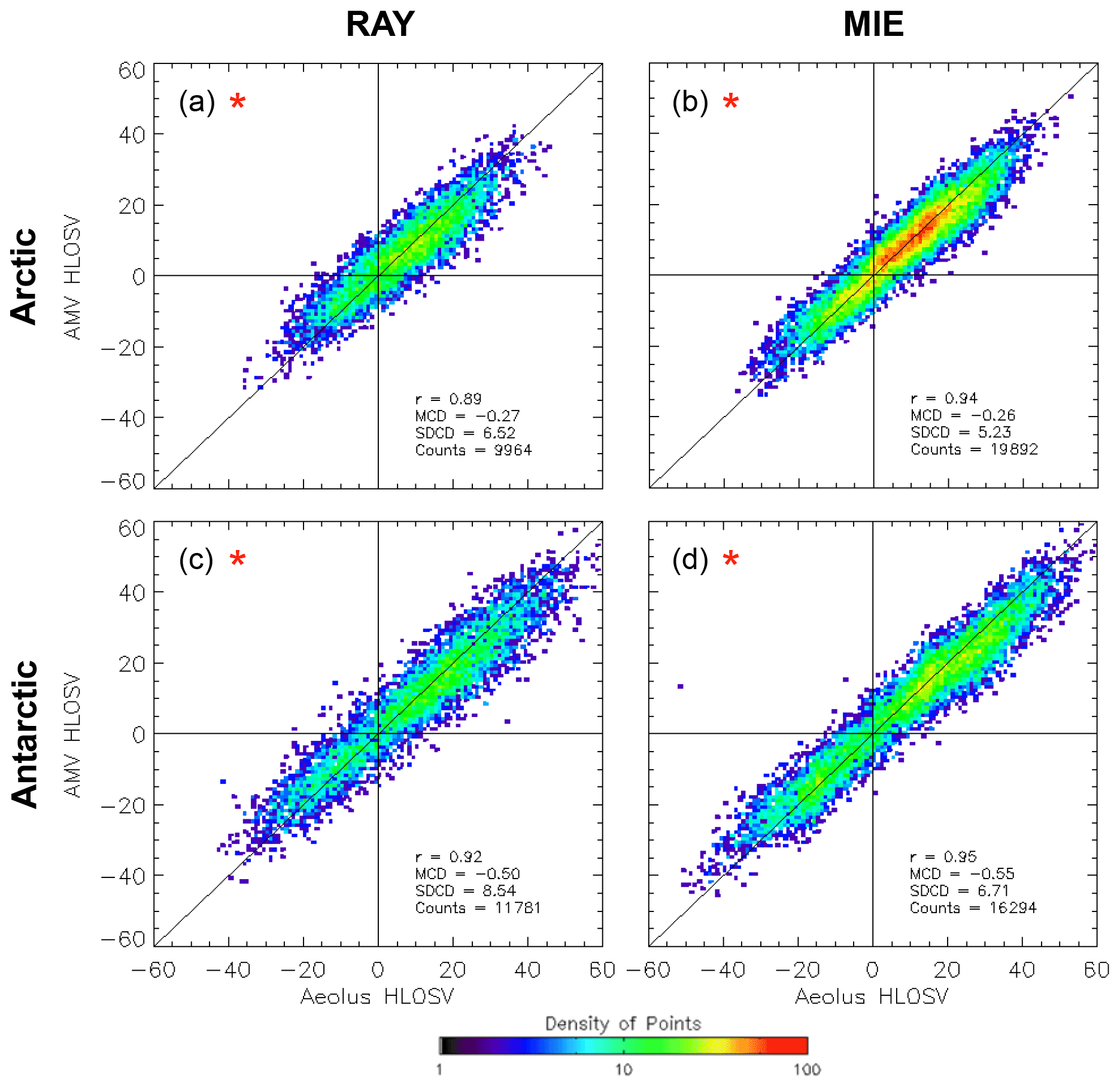
Figure 12Density scatterplots of co-located IR–window AMVs from all available LEO satellites and RAY (a, c) and MIE (b, d) winds. Comparisons in the (a–b) Arctic (north of 60∘ N) and (c–d) Antarctic (south of 60∘ S) are shown. Colors indicate total number of co-located observation pairs within the cells plotted, which are 1 m s−1 on a side. Sample statistics are displayed in the bottom right corner of each panel. Horizontal and vertical zero lines are plotted in black, as is the diagonal one-to-one line. A red star denotes statistical significance at the 95 % level, using the paired two-tailed Student's t test. HLOSV units are m s−1.
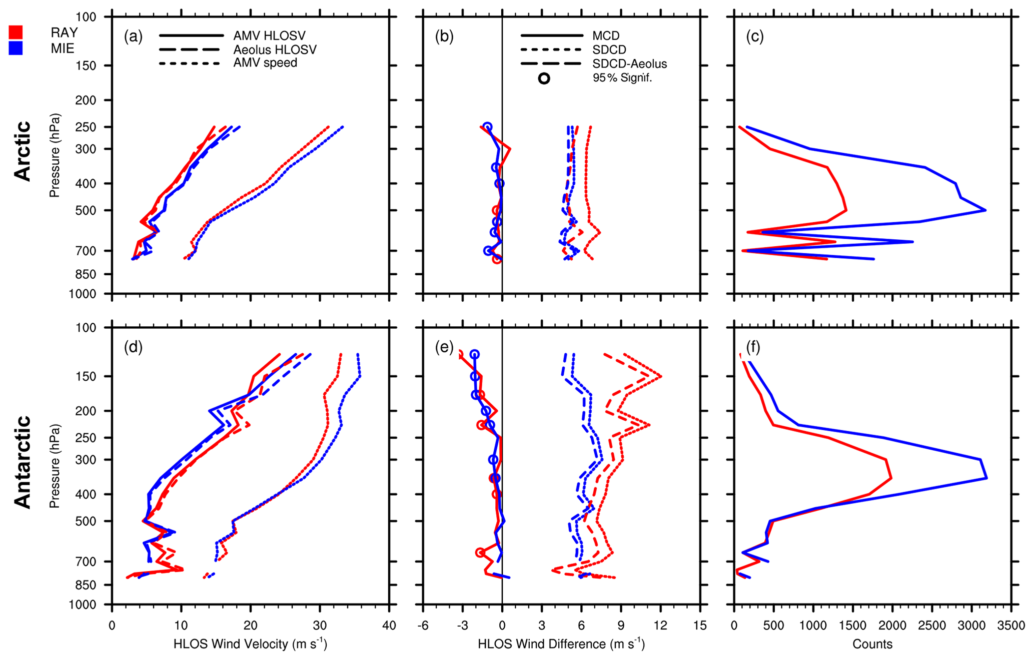
Figure 13Vertical profiles of co-located LEO AMVs and RAY (red) and MIE (blue) winds. The top row shows the Arctic (north of 60∘ N), (a) mean AMV HLOSV (solid lines), Aeolus HLOSV (long dashed lines; m s−1), and mean AMV wind speed (short dashed lines; m s−1), (b) MCDs (solid), SDCDs (short dashed), and AMV HLOSV error, as represented by SDCD–Aeolus L2B uncertainty (long dashed; m s−1), and (c) co-location counts. Panels (d–f) are as in panels (a–c) but for the Antarctic (south of 60∘ S). Colored open circles indicate levels where MCDs are statistically significant at the 95 % level (p value < 0.05), using the paired Student's t test. Vertical zero lines are displayed in the center panels in black. Levels with observation counts > 25 are plotted.
As was done for the GOES-16 case study, we examine the vertical differences between all LEO AMVs and Aeolus winds to ascertain how AMVs characterize the dynamical flow at the poles (Fig. 13). RAY (red colors) and MIE comparisons (blue colors) are presented together. AMV HLOSV and Aeolus HLOSV profiles are similar throughout the vertical, with notably larger MCDs in the Antarctic at upper levels. In the Arctic (Fig. 13, top row), MIE winds and co-located AMVs depict faster motions relative to RAY comparisons. Statistically significant MCDs are of the order of −0.5 m s−1 at mid-levels where co-location counts peak, representing slower AMV winds relative to Aeolus. The MCDs become larger (more negative) nearer the tropopause (around 300–250 hPa), where HLOSVs reach upwards of 15 m s−1, and AMV wind speeds reach 30 m s−1, while corresponding total SDCDs are generally constant but smaller for MIE (∼ 5 m s−1) than RAY (∼ 7 m s−1). Removal of the Aeolus uncertainty yields adjusted SDCD profiles that are nearly equal to the total MIE SDCDs, indicating the higher accuracy of MIE winds in the Arctic at all levels, including those with higher wind speeds. This independence of Aeolus MIE uncertainty to changes in wind speed is clear in Fig. 14a, where Aeolus MIE errors are shown to be smaller relative to RAY and remain relatively constant with increasing AMV wind speeds. In addition, the near doubling of MIE co-location counts at mid-levels relative to RAY (Fig. 13c) could be due to increased cloudiness associated with more moisture availability in the Arctic summer (Alekseev et al., 2018).
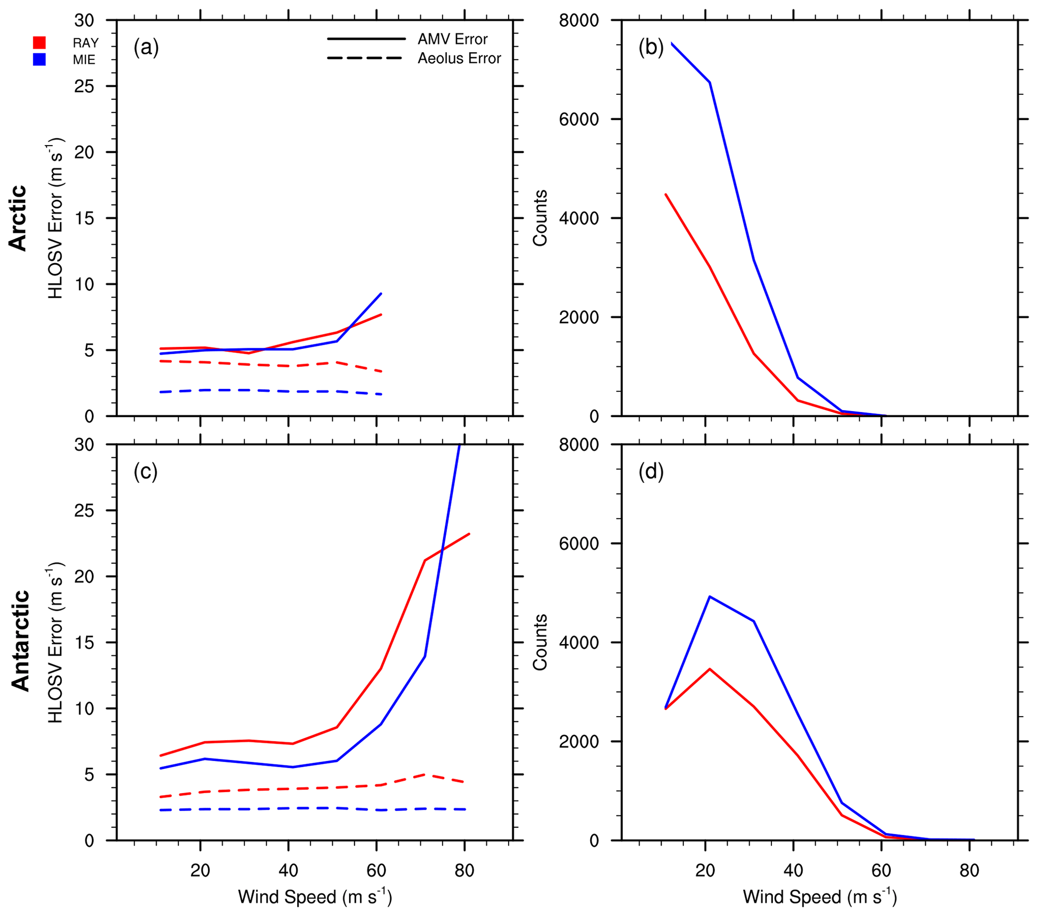
In the Antarctic (Fig. 13, bottom row), HLOSVs increase from 5 m s−1 at mid-levels to nearly 30 m s−1 at very high levels (∼ 150 hPa), and RAY comparisons are shown to capture generally faster motions throughout much of the vertical column. MCDs are small (around −0.5 m s−1) at mid-levels, where co-location counts peak but are larger aloft and represent over 10 % of the corresponding HLOSV. Larger MCDs aloft could be attributed to the wind shear height assignment error effect related to the strengthening of the Antarctic polar vortex in late winter/early spring. As shown in the Arctic, MIE comparisons in the Antarctic have smaller total SDCDs (5–7 m s−1) than RAY (6–12 m s−1, respectively) throughout the vertical; however, Antarctic MIE and RAY SDCDs are larger than in the Arctic and appear to increase with height. Higher SDCD values at upper levels may be attributed to larger AMV and Aeolus errors in layers of faster winds. Adjusted SDCDs and Aeolus error estimates for RAY comparisons increase with increasing AMV wind speed (Fig. 14c), suggesting that both AMV errors and Aeolus errors in layers of high winds and strong shear contribute to the larger SDCDs observed in the Antarctic.
This study summarizes statistical comparisons of AMVs with the novel Aeolus L2B HLOS winds for samples stratified by specific sets of conditions and discusses their relationship to known AMV characteristics. Because Aeolus observes the HLOSVs – the horizontal wind projected onto the HLOS of the DWL – derived from the detection of molecular and aerosol backscattering signals, the assessments of mean co-location differences (AMV minus Aeolus) and SD of the differences are all in terms of AMV winds projected onto the co-located Aeolus HLOS. In the tropics, due to the Aeolus observing geometry, HLOSV represents the zonal wind. Aeolus HLOSV profiles utilized in this study are classified as RAY or Rayleigh-clear winds (representing mostly clear-sky scenes) and MIE or Mie-cloudy winds (representing cloudy scenes only). Winds quality controlled (QC'd) following recommendations by the ESA for Aeolus and by the user community for the satellite winds are retained for analysis. The performance of QC'd AMVs relative to co-located QC'd Aeolus winds are characterized by analyzing sample statistics of the co-located differences, which is AMV HLOSV minus Aeolus HLOSV. These statistics should not be strictly interpreted as overall AMV performance, as differences arise from errors in both AMVs and Aeolus winds and from representativeness and co-location errors.
Comparisons of GOES-16 AMVs and IR cloud-tracked AMVs from LEO satellites are assessed to estimate the dependence of AMVs on different combinations of conditions including Aeolus observing mode/scene type (clear or cloudy), AMV type (IR, WVcloud, and WVclear), and geographic region (tropics and extratropics for GOES-16, Arctic, and Antarctic polar regions for LEO). GOES-16 was chosen as a representative of GEO performance, as the AMVs exhibit high correlations with Aeolus, relatively low MCDs, and SDCDs and have a large sample size from which to compute robust statistics. The summary assessment of all LEO AMVs provides a unique, comprehensive perspective on the characteristics of polar AMVs using a larger sample of co-located Aeolus wind profiles relative to other available datasets, e.g., rawinsonde profile data. Vertical distributions of differences in HLOSV are examined, as this perspective has the potential to provide additional insight into how accurately each AMV type represents the horizontal flow in the vertical. AMVs exhibit different characteristics in clear and cloudy scenes that vary with geographic region and in the vertical, which is in agreement with the findings in Velden et al. (1997), Posselt et al. (2019), and others. Overall, GEO and LEO AMVs are found to compare as well with Aeolus RAY and MIE winds as they do to conventional data sources and NWP products, particularly in the tropics, NH extratropics, in the Arctic, and at mid- to upper-levels in both clear and cloudy scenes. SH comparisons generally exhibit larger-than-expected SDCDs that could be attributed to larger height assignment errors and larger representativeness and co-location errors in regions of high winds and strong vertical wind shear.
The main findings from comparing GOES-16 AMVs with RAY and MIE winds are the following. Aeolus MIE winds show great potential value as a comparison standard to characterize AMVs. MIE comparisons generally exhibit smaller biases and uncertainties compared to RAY, reflecting the higher accuracy of MIE winds and AMVs in cloudy scenes and larger co-location errors for RAY winds in cloudy scenes. This is attributed to a combination of smaller Aeolus MIE uncertainties and smaller co-location/representativeness errors due to the cloudy/cloudy sampling effect; that is, the fact that both Aeolus and AMV winds are, by definition, sampling similar cloudy scenes at similar altitudes. The contribution of Aeolus MIE uncertainty to the overall SDCDs is small; in fact, removal of Aeolus uncertainties further reduces the small MIE SDCDs without much change to its vertical distribution, suggesting that, for MIE comparisons, the dominant factors contributing to the total error consist of AMV random errors and representativeness/co-location errors. Additionally, the AMV–Aeolus MIE comparisons depict a relatively new finding that is also noted in Cotton et al. (2020, 2021) and is largely thought to be attributed to AMV height assignment errors, i.e., a negative speed bias in the IR and WVcloud AMVs in the tropics. The fact that comparisons with Aeolus exhibit this feature hints at the usefulness of Aeolus MIE winds as a standard for comparison to characterize AMVs. (It should be noted that, because the period of study is relatively short, the datasets are not large enough to examine in detail many of the features identified and studied in the NWP SAF AMV monitoring. However, it could be possible to verify the identification of such features in AMV comparisons with Aeolus observations by using a larger co-location dataset, which the authors are preparing and making publicly available.)
Regarding GOES-16 RAY comparisons, sampling differences may play a role in the higher correlation between Aeolus RAY winds and WVclear AMVs, since they both represent similar clear-sky scenes. This is especially true in the tropics and NH extratropics where MCDs are small, and SDCDs are comparable to AMV error values compared with high-quality rawinsonde winds. It is likely that co-location errors play a larger role in the RAY SDCDs for IR and WVcloud AMVs due to the cloudy/clear sampling effect, where clear-sky Aeolus winds are co-located with cloudy AMVs and, thereby, observe different scenes, yielding larger errors. In addition, the removal of Aeolus uncertainties from the total SDCDs considerably reduces the RAY SDCDs, particularly for IR and WVcloud comparisons, indicating that Aeolus contributes a substantial fraction of the total SDCDs in the presence of clouds.
Polar AMVs have smaller MCDs for MIE compared to RAY, although Antarctic AMVs have larger SDCDs than the Arctic. In fact, GEO and LEO comparisons in the SH/Antarctic exhibit the largest SDCDs of all regions examined. Large wind shear is evident in the SH/Antarctic throughout much of the atmospheric column, and this can dramatically affect AMV height assignment errors. Indeed, AMV errors are shown to generally increase with increasing AMV wind speed, as do corresponding Aeolus errors for RAY winds, suggesting that both contribute to the larger SDCDs observed in layers of high wind speed. Additionally, larger RAY MCDs aloft could be attributed to larger co-location/representativeness errors due to IR AMVs and RAY winds viewing different scenes. The possible mischaracterization of very cold surface temperatures as clouds may also be a factor. For GOES-16 MIE comparisons in the SH, AMV errors are larger and increase with AMV speeds > 40 m s−1, while Aeolus MIE errors are small and remain relatively constant. This implies that the large systematic differences in MCDs at upper levels in the SH extratropics are most probably attributed to larger AMV errors in combination with the wind-shear height assignment error effect.
The use of Aeolus winds as a benchmark dataset for the comparative assessment of AMVs has valuable implications for future research, including the validation of 3D winds and the use of such data in NWP. For example, the findings presented here contribute to the ongoing development of a feature track correction (FTC) observation operator to account for AMV height assignment and other biases in data assimilation (Hoffman et al., 2022). Future studies should use larger datasets like the ones that the authors are preparing to compare clear-scene AMVs with Aeolus Rayleigh-clear winds only and cloudy-scene AMVs with Aeolus Mie-cloudy winds only. Such studies are anticipated to yield additional insights into the seasonal performance of AMV characteristics representing different dynamical features in clear and cloudy scenes and how this might be accounted for or improved upon in AMV algorithms. Moreover, the robustness of dynamical features identified in AMV monitoring could be further validated following this approach. In addition, Aeolus Mie-cloudy comparisons using larger datasets are expected to have a significant impact towards improving our understanding and characterization of AMV quality in cloudy scenes, given the cloudy/cloudy sampling effect and the small contribution of Aeolus Mie-cloudy error to the total SDCDs throughout the vertical in all geographic regions, implying that the corresponding adjusted SDCDs better depict true AMV uncertainty. This is especially critical where AMV height assignment errors are likely large but Aeolus Mie-cloudy errors are small and remain relatively constant with respect to height and AMV wind speed, e.g., in layers of strong vertical wind shear and in the SH. One lesson learned from this study is that QC of both AMV and Aeolus observations is critical and largely improves the results. The Aeolus project has done much to eliminate errors of all types, but some improvements are expected, e.g., via the removal of DWL instrument calibration-dependent error. Furthermore, some of the bias corrections currently applied depend on ECMWF forecasts, and the analysis of H. Liu et al. (2022) demonstrates that additional bias corrections for Aeolus are possible and that such corrections can improve NWP analysis and forecast results (Garrett et al., 2022).
Formulae for the statistics used in this study are presented here. Since HLOSV is a scalar, these formulae correspond directly with the standard textbook formulae. The co-location database is composed of pairs (xi,yi) for i=1, n, where n is the number of co-locations, i is the co-location index, x is the Aeolus HLOSV, and y is the AMV HLOSV. The correlation (r) between co-located HLOSVs describes the overall relation of AMVs to Aeolus and is defined as follows:
Overbars denote sample means. The corresponding standard deviations sx and sy are defined as follows:
where w can equal x or y. The co-location difference (CD) is the difference in m s−1 between each pair of co-located AMV HLOSV and Aeolus HLOSV, as follows:
and the mean (MCD) represents the sample mean of the CD for select conditions, such as a specific geographic region, pressure level, AMV type, or Aeolus observing mode.
Using Eq. (A2), we can define the corresponding SDCDs in terms of CD as follows:
Finally, the adjusted SDCD, sadj, is defined, in the following, as the SDCD with the corresponding Aeolus error estimate sx removed:
The Aeolus L2B Earth Explorer data used in this study are publicly available and can be accessed via the ESA Aeolus Online Dissemination System (https://aeolus-ds.eo.esa.int/oads/access/; ESA, 2020). The NCEP SATWND BUFR AMV dataset can be provided by the corresponding author (katherine.lukens@noaa.gov) upon request. Additionally, the authors are preparing an Aeolus–AMV co-location dataset that will be provided upon request.
KG and KI proposed the project as co-investigators and provided the expertise that guided this work. BH and DS developed the co-location algorithm used. KEL performed most of the work that included the implementation of the co-location algorithm and comparison analysis. DS, RNH, and HL provided additional intellectual support that considerably improved the article. KEL prepared the paper, with contributions from all co-authors.
The contact author has declared that neither they nor their co-authors have any competing interests.
The scientific results and conclusions, as well as any views or opinions expressed herein, are those of the authors and do not necessarily reflect those of NOAA or the U.S. Department of Commerce.
Publisher’s note: Copernicus Publications remains neutral with regard to jurisdictional claims in published maps and institutional affiliations.
This article is part of the special issue “Aeolus data and their application (AMT/ACP/WCD inter-journal SI)”. It is not associated with a conference.
Careful and helpful anonymous referee comments considerably improved the article; the reviewer comments and active dialog to clarify these comments were extremely useful in this regard. The authors thank their colleagues at NOAA/NESDIS/STAR, for overseeing this work, and Mike Hardesty, Iliana Genkova, and the rest of the U.S. Aeolus Cal/Val team, for the guidance and support. The University of Wisconsin-Madison S4 supercomputing system (Boukabara et al., 2016) was used in this work. The authors acknowledge support from the NOAA/NESDIS Office of Projects, Planning, and Acquisition (OPPA) Technology Maturation Program (TMP), through CICS and CISESS at the University of Maryland/ESSIC and CIMSS at the University of Wisconsin-Madison.
This research has been supported by the National Oceanic and Atmospheric Administration (grant nos. NA14NES4320003, NA19NES4320002, and NA20NES4320003).
This paper was edited by Ad Stoffelen and reviewed by two anonymous referees.
Abdalla, S., de Kloe, J., Flament, T., Krisch, I., Marksteiner, U., Reitebuch, O., Rennie, M., Weiler, F., and Witschas, B.: Verification report of first Reprocessing campaign for FM-B covering the time period 2019-06 to 2019-12. Tech. rep., Aeolus Data Innovation Science Cluster DISC, Version 1.0, REF: AED-TN-ECMWF-GEN-040, internal document available for registered Aeolus Cal/Val teams, summary of this document available at: https://earth.esa.int/eogateway/documents/20142/0/Aeolus-Summary-Reprocessing-1-DISC.pdf (last access: 4 January 2022), 2020.
Alekseev, G., Kuzmina, S., Bobylev, L., Urazgildeeva, A., and Gnatiuk, N.: Impact of atmospheric heat and moisture transport on the Arctic warming, Int. J. Climatol., 39, 3582–3592, https://doi.org/10.1002/joc.6040, 2018.
Bedka, K. M., Velden, C. S. Petersen, R. A. Feltz, W. F., and Mecikalski, J. R.: Comparisons of Satellite-Derived Atmospheric Motion Vectors, Rawinsondes, and NOAA Wind Profiler Observations, J. Appl. Meteorol. Clim., 48, 1542–1561, https://doi.org/10.1175/2009JAMC1867.1, 2009.
Berger, H., Langland, R., Velden, C. S., Reynolds, C. A., and Pauley, P. M.: Impact of enhanced satellite-derived atmospheric motion vector observations on numerical tropical cyclone track forecasts in the western North Pacific during TPARC/TCS-08, J. Appl. Meteorol. Clim., 50, 2309–2318, https://doi.org/10.1175/JAMC-D-11-019.1, 2011.
Bormann, N., Kelly, G., and Thépaut, J.-N.: Characterising and correcting speed biases in atmospheric motion vectors within the ECMWF system, in: Sixth Int. Winds Workshop, 7–10 May 2002, Madison, WI, USA, EUMETSAT, 113–120, http://cimss.ssec.wisc.edu/iwwg/iww6/session3/bormann_1_bias.pdf (last access: 18 April 2021), 2002.
Bormann, N., Saarinen, S., Kelly, G., and Thepaut, J.-N.: The Spatial Structure of Observation Errors in Atmospheric Motion Vectors from Geostationary Satellite Data, Mon. Weather Rev., 131, 706–718, https://doi.org/10.1175/1520-0493(2003)131<0706:TSSOOE>2.0.CO;2, 2003.
Boukabara, S. A., Zhu, T., Tolman, H. L., Lord, S., Goodman, S., Atlas, R., Goldberg, M., Auligne, T., Pierce, B., Cucurull, L., Zupanski, M., Zhang, M., Moradi, I., Otkin, J., Santek, D., Hoover, B., Pu, Z., Zhan, X., Hain, C., Kalnay, E., Hotta, D., Nolin, S., Bayler, E., Mehra, A., Casey, S. P. F., Lindsey, D., Grasso, L., Kumar, V. K., Powell, A., Xu, J., Greenwald, T., Zajic, J., Li, J., Li, J., Li, B., Liu, J., Fang, L., Wang, P., and Chen, T.-C.: S4: An O2R/R2O infrastructure for optimizing satellite data utilization in NOAA numerical modeling systems. a step toward bridging the gap between research and operations, B. Am. Meteorol. Soc., 97, 2359–2378, https://doi.org/10.1175/bams-d-14-00188.1, 2016.
Chen, S., Cao, R., Xie, Y., Zhang, Y., Tan, W., Chen, H., Guo, P., and Zhao, P.: Study of the seasonal variation in Aeolus wind product performance over China using ERA5 and radiosonde data, Atmos. Chem. Phys., 21, 11489–11504, https://doi.org/10.5194/acp-21-11489-2021, 2021.
Conger, K.: “Master”, “slave” and the fight over offensive terms in computing, The New York Times, 13 April 2021, https://www.nytimes.com/2021/04/13/technology/racist-computer-engineering-terms-ietf.html (last access: 4 January 2022), 2021.
Cordoba, M., Dance, S. L., Kelly, G. A., Nichols, N. K., and Walker, J. A.: Diagnosing atmospheric motion vector observation errors for an operational high-resolution data assimilation system, Q. J. Roy. Meteor. Soc., 143, 333–341, https://doi.org/10.1002/qj.2925, 2017.
Cotton, J., Doherty, A., Lean, K., Forsythe, M., and Cress, A.: NWP SAF AMV monitoring: the 9th Analysis Report (AR9), Tech. rep., NWP SAF, Version 1.0, REF: NWPSAF-MO-TR-039, https://nwp-saf.eumetsat.int/site/monitoring/winds-quality-evaluation/amv/amv-analysis-reports/ (last access: 9 May 2021), 2020.
Cotton, J., Doherty, A., and Lean, K.: Characterising AMV errors using the NWP SAF monitoring, in: 15th IWWG Workshop, 12–16 April 2021, Virtual, https://www.ssec.wisc.edu/meetings/iwwg/2021-meeting/presentations/oral-cotton/ (last access: 3 January 2022), 2021.
Daniels, J., Bresky, W., Bailey, A., Allegrino, A., Wanzong, S., and Velden, C.: Introducing Atmospheric Motion Vectors Derived from the GOES-16 Advanced Baseline Imager (ABI), in: 14th International Winds Workshop, 17 June 2020, Jeju City, South Korea, CIMSS, ESA, http://cimss.ssec.wisc.edu/iwwg/iww14/talks/01_Monday/1400_IWW14_ABI_AMVs_Daniels.pdf (last access: 20 February 2021), 2018.
de Kloe, J., Stoffelen, A., Tan, D., Andersson, E., Rennie, M., Dabas, A., Poli, P., and Huber, D.: Aeolus Data Innovation Science Cluster DISC ADM-Aeolus Level-2B/2C Processor Input/Output Data Definitions Interface Control Document. Tech. rep., KMNI, Aeolus, DISC, REF: AED-SD-ECMWF-L2B-037, https://earth.esa.int/eogateway/documents/20142/37627/Aeolus-L2B-2C-Input-Output-DD-ICD.pdf (last access: 17 April 2021), 2020.
ESA-ESRIN: Aeolus Cal/Val and Science Workshop 2019 Summary, in: Aeolus CAL/VAL and Science Workshop 2019, 26–29 March 2019, Frascati, Italy, https://az659834.vo.msecnd.net/eventsairwesteuprod/production-nikal-public/3cb005cf00ea441d97eb5cadb5f3c78c (last access: 25 April 2022), 2019.
European Space Agency (ESA): Aeolus L2B Earth Explorer data set, ESA [data set], https://aeolus-ds.eo.esa.int/oads/access/ (last access: 25 February 2021), 2020.
Garrett, K., Liu, H., Ide, K., Hoffman, R., and Lukens, K. E.: Optimization and Impact Assessment of Aeolus HLOS Wind Data Assimilation in NOAA's Global Forecast System, Q. J. Roy. Meteor. Soc., in review, 2022.
Grieger, J., Leckebusch, G. C., and Ulbrich, U.: Net Precipitation of Antarctica: Thermodynamical and Dynamical Parts of the Climate Change Signal, J. Climate, 29, 907–924, https://doi.org/10.1175/JCLI-D-14-00787.1, 2016.
Hoffman, R. N., Lukens, K. E., Ide, K., and Garrett, K.: A Collocation Study of Atmospheric Motion Vectors (AMVs) Compared to Aeolus Wind Profiles with a Feature Track Correction (FTC) Observation Operator, Q. J. Roy. Meteor. Soc., 148, 321–337, https://doi.org/10.1002/qj.4207, 2022.
Hoskins, B. J. and Hodges, K. I.: A new perspectives on Southern Hemisphere storm tracks, J. Climate, 18, 4108–4129, https://doi.org/10.1175/JCLI3570.1, 2005.
Jung, J., Le Marshall, J., Daniels, J., and Riishojgaard, L. P.: Investigating height assignment type errors in the NCEP global forecasting system, in: 10th International Wind Workshop, 22–26 February 2010, Tokyo, Japan, EUMETSAT P.56, https://www-cdn.eumetsat.int/files/2020-04/pdf_conf_p56_s3_04_jung_v.pdf (last access: 22 February 2021), 2010.
Key, J., Santek, D., and Dworak, R.: Polar winds from shortwave infrared cloud tracking, in: Proc. 13th Int. Winds Workshop, Monterey, California, USA, 1–6, https://www.researchgate.net/profile/Jeffrey-Key-2/publication/309727571_Polar_winds_from_shortwave_infrared_cloud_tracking/links/581f84da08aea429b29907fd/Polar-winds-from-shortwave-infrared-cloud-tracking.pdf (last access: 7 September 2021), 2016.
Le Marshall, J., Jung, J., Zapotocny, T., Redder, C., Dunn, M., Daniels, J., and Riishojgaard, L. P.: Impact of MODIS atmospheric motion vectors on a global NWP system, Aust. Met. Mag., 57, 45–51, http://citeseerx.ist.psu.edu/viewdoc/download?doi=10.1.1.222.6537&rep=rep1&type=pdf (last access: 9 May 2021), 2008.
Liu, B., Guo, J., Gong, W., Zhang, Y., Shi, L., Ma, Y., Li, J., Guo, X., Stoffelen, A., de Leeuw, G., and Xu, X.: Intercomparison of wind observations from ESA’s satellite mission Aeolus, ERA5 reanalysis and radiosonde over China, Atmos. Meas. Tech. Discuss. [preprint], https://doi.org/10.5194/amt-2022-26, in review, 2022.
Liu, H., Garrett, K., Ide, K., Hoffman, R., and Lukens, K.: A Statistically Optimal Analysis of Systematic Differences between Aeolus HLOS Winds and NOAA’s Global Forecast System, Atmos. Meas. Tech. Discuss. [preprint], https://doi.org/10.5194/amt-2022-20, in review, 2022.
Lux, O., Lemmerz, C., Weiler, F., Marksteiner, U., Witschas, B., Rahm, S., Geiß, A., and Reitebuch, O.: Intercomparison of wind observations from the European Space Agency's Aeolus satellite mission and the ALADIN Airborne Demonstrator, Atmos. Meas. Tech., 13, 2075–2097, https://doi.org/10.5194/amt-13-2075-2020, 2020.
Martin, A., Weissmann, M., Reitebuch, O., Rennie, M., Geiß, A., and Cress, A.: Validation of Aeolus winds using radiosonde observations and numerical weather prediction model equivalents, Atmos. Meas. Tech., 14, 2167–2183, https://doi.org/10.5194/amt-14-2167-2021, 2021.
Nakamura, H. and Shimpo, A.: Seasonal Variations in the Southern Hemisphere Storm Tracks and Jet Streams as Revealed in a Reanalysis Dataset, J. Climate, 17, 1828–1844, https://doi.org/10.1175/1520-0442(2004)017<1828:SVITSH>2.0.CO;2, 2004.
National Academies of Sciences, Engineering, and Medicine: Thriving on Our Changing Planet: A Decadal Strategy for Earth Observation from Space. National Academies Press, Washington, DC, USA, https://doi.org/10.17226/24938, 2018.
Posselt, D., Wu, L., Mueller, K., Huang, L., Irion, F. W., Brown, S., Su, H., Santek, D., and Velden, C. S.: Quantitative Assessment of State-Dependent Atmospheric Motion Vector Uncertainties. J. Appl. Meteorol. Clim., 58, 2479–2495, https://doi.org/10.1175/JAMC-D-19-0166.1, 2019.
Reitebuch, O., Lemmerz, C., Nagel, E., Paffrath, U., Durand, Y., Endemann, M., Fabre, F., and Chaloupy, M.: The Airborne Demonstrator for the Direct-Detection Doppler Wind Lidar ALADIN on ADM-Aeolus. Part I: Instrument Design and Comparison to Satellite Instrument, J. Atmos. Ocean. Tech., 26, 2501–2515, https://doi.org/10.1175/2009JTECHA1309.1, 2009.
Rennie, M. and Isaksen, L.: The NWP impact of Aeolus Level-2B winds at ECMWF. Tech. rep., Aeolus Data Innovation Science Cluster DISC, Ref: AED-TN-ECMWF-NWP-025, https://doi.org/10.21957/alift7mhr, 2020a.
Rennie, M. and Isaksen, L.: Assessment of the Impact of Aeolus Doppler Wind Lidar Observations for Use in Numerical Weather Prediction at ECMWF, in: EGU 2020, 28 April 2020, Virtual, Copernicus, https://presentations.copernicus.org/EGU2020/EGU2020-5340_presentation.pdf (last access: 20 February 2021), 2020b.
Rennie, M., Tan, D., Andersson, E., Poli, P., Dabas, A., de Kloe, J., and Stoffelen, A.: Aeolus Level-2B Algorithm Theoretical Basis Document: Mathematical Description of the Aeolus Level-2B Processor, Tech. rep., ESA, Version 3.4, Ref: AED-SD-ECMWF-L2B-038, https://earth.esa.int/eogateway/documents/20142/37627/Aeolus-L2B-Algorithm-ATBD.pdf, last access: 20 November 2020.
Salonen, K., Cotton, J., Bormann, N., and Forsythe, M.: Characterizing AMV height-assignment error by comparing best-fit pressure statistics from the Met Office and ECMWF data assimilation systems, J. Appl. Meteorol. Clim., 54, 225–242, https://doi.org/10.1175/JAMC-D-14-0025.1, 2015.
Santek, D., García-Pereda, J., Velden, C., Genkova, I., Wanzong, S., Stettner, D., and Mindock, M.: A new atmospheric motion vector intercomparison study, in: 12th International Winds Workshop, 16–20 June 2014, Copenhagen, Denmark, CIMSS, Technical Report, http://www.nwcsaf.org/aemetRest/downloadAttachment/225 (last access: 18 December 2020), 2014.
Santek, D., Dworak, R., Nebuda, S., Wanzong, S., Borde, R., Genkova, I., García-Pereda, J., Negri, R. G., Carranza, M., Nonaka, K., Shimoji, K., Oh, S. M., Lee, B.-I., Chung, S.-R., Daniels, J., and Bresky, W.: 2018 Atmospheric Motion Vector (AMV) Intercomparison Study, Remote Sens., 11, 2240, https://doi.org/10.3390/rs11192240, 2019.
Santek, D., Hoover, B., Zhang, H., and Moeller, C.: Evaluation of Aeolus Winds by Comparing to AIRS 3D Winds, Rawinsondes, and Reanalysis Grids, in: 15th International Winds Workshop, 12–16 April 2021, Virtual, CIMSS, https://www.ssec.wisc.edu/meetings/iwwg/2021-meeting/presentations/oral-santek/, last access: 9 May 2021.
Schmetz, J., Holmlund, K., Hoffman, J., Strauss, B., Mason, B., Gaertner, V., Koch, A., and Van De Berg, L.: Operational cloud-motion winds from Meteosat infrared images, J. Appl. Meteorol., 32, 1206–1225, https://doi.org/10.1175/1520-0450(1993)032<1206:OCMWFM>2.0.CO;2, 1993.
Schmetz, J., Holmlund, K., Roesli, H. P., and Levizzani, V.: On the Use of Rapid Scans, Proceedings of the Fifth International Winds Workshop, Lorne, Australia, 28 February–3 March 2000, EUM P28, EUMETSAT, 227–234, http://cimss.ssec.wisc.edu/iwwg/iww5/S5-2_Schmetz-OnTheUse.pdf (last access: 4 January 2022), 2000.
Stoffelen, A., Pailleux, J., Källén, E., Vaughan, J. M., Isaksen, L., Flamant, P., Wergen, W., Andersson, E., Schyberg, H., Culoma, A., Meynart, R., Endemann, M., and Ingmann, P.: The atmospheric dynamics mission for global wind field measurement, B. Am. Meteorol. Soc., 86, 73–87, https://doi.org/10.1175/BAMS-86-1-73, 2005.
Straume, A. G., Elfving, A., Wernham, D., Kanitz, T., de Bruin, F., Buscaglione, F., von Bismarck, J., and Lengert, W.: Status of ESA's Doppler Wind Lidar Mission Aeolus, in: 14th International Winds Workshop, 23–27 April 2018, Jeju City, South Korea, ESA, http://cimss.ssec.wisc.edu/iwwg/iww14/talks/04_Thursday/1000_IWW14_Aeolus_Straume.pdf (last access: 28 August 2019), 2018.
Straume, A. G., Rennie, M., Isaksen, L., de Kloe, J., Marseille, G.-J., Stoffelen, A., Flament, T., Stieglitz, H., Dabas, A., Huber, D., Reitebuch, O., Lemmerz, C., Lux, O., Marksteiner, U., Weiler, F., Witschas, B., Meringer, M., Schmidt, K., Nikolaus, I., Geiss, A., Flamant, P., Kanitz, T., Wernham, D., von Bismarck, J., Bley, S., Fehr, T., Floberghagen, R., and Parinello, T.: ESA's space-based Doppler wind lidar mission Aeolus – first wind and aerosol product assessment results, EPJ Web Conferences, 237, 01007, https://doi.org/10.1051/epjconf/202023701007, 2020.
Straume, A. G., Parrinello, T., von Bismarck, J., Bley, S., Ehlers, F., and the Aeolus teams: ESA's Wind Lidar Mission Aeolus – status and scientific exploitation after 2.5 years in space, in: 15th International Winds Workshop, 12–16 April 2021, Virtual, ESA, https://www.ssec.wisc.edu/meetings/wp-content/uploads/sites/33/2021/02/IWW15_Presentation_AG_Straume.pdf, last access: 9 May 2021.
Straume-Lindner, A. G.: Aeolus Sensor and Product Description. Tech. rep., European Space Agency – European Space Research and Technology Centre, the Netherlands, REF: AE-SU-ESA-GS-000, https://earth.esa.int/eogateway/documents/20142/37627/Aeolus-Sensor-and-Product-Description.pdf (last access: 9 May 2021), 2018.
Trenberth, K.: Storm tracks in the Southern Hemisphere, J. Atmos. Sci., 48, 2159–2178, https://doi.org/10.1175/1520-0469(1991)048<2159:STITSH>2.0.CO;2, 1991.
Velden, C., Daniels, J., Stettner, D., Santek, D., Key, J., Dunion, J., Holmlund, K., Dengel, G., Bresky, W., and Menzel, P.: Recent innovations in deriving tropospheric winds from meteorological satellites, B. Am. Meteorol. Soc., 86, 205–223, https://doi.org/10.1175/BAMS-86-2-205, 2005.
Velden, C. S. and Bedka, K. M.: Identifying the Uncertainty in Determining Satellite-Derived Atmospheric Motion Vector Height Attribution, J. Meteorol. Clim., 48, 450–463, https://doi.org/10.1175/2008JAMC1957.1, 2009.
Velden, C. S. and Holmlund, K.: Report from the working group on verification and quality indices (WG II), in: 4th International Winds Workshop, 20–23 October 1998, Saanenmöser, Switzerland, EUMETSAT, https://cimss.ssec.wisc.edu/iwwg/iww4/p19-20_WGReport3.pdf (last access: 5 January 2022), 1998.
Velden, C. S., Hayden, C. M., Nieman, S. J., Menzel, W. P., Wanzong, S., and Goerss, J. S.: Upper-tropospheric winds derived from geostationary satellite water vapor observations, B. Am. Meteorol. Soc., 78, 173–195, https://doi.org/10.1175/1520-0477(1997)078<0173:UTWDFG>2.0.CO;2, 1997.
von Bremen, L.: Using simulated satellite images to improve the characterization of Atmospheric Motion Vectors (AMVs) and their errors for Numerical Weather Prediction, NWP SAF, Version 1.4, REF: NWPSAF-EC-VS-015, http://research.metoffice.gov.uk/research/interproj/nwpsaf/vs.html (last access: 7 September 2021), 2008.
Weiler, F., Rennie, M., Kanitz, T., Isaksen, L., Checa, E., de Kloe, J., Okunde, N., and Reitebuch, O.: Correction of wind bias for the lidar on board Aeolus using telescope temperatures, Atmos. Meas. Tech., 14, 7167–7185, https://doi.org/10.5194/amt-14-7167-2021, 2021.
Wilks, D.: Statistical Methods in the Atmospheric Sciences, vol. 100, 3rd edn., Academic Press, ISBN 9780123850225, 2011.
Wu, T.-C., Liu, H., Majumdar, S. J., Velden, C. S., and Anderson, J. L.: Influence of assimilating satellite-derived atmospheric motion vector observations on numerical analyses and forecasts of tropical cyclone track and intensity, Mon. Weather Rev., 142, 49–71, https://doi.org/10.1175/MWR-D-13-00023.1, 2014.
Zuev, V. V. and Savelieva, E.: The cause of the spring strengthening of the Antarctic polar vortex, Dyn. Atmos. Oceans, 87, 101097, https://doi.org/10.1016/j.dynatmoce.2019.101097, 2019.
The meaning of the term “blocklist” is identical to the term “blacklist”; however, “blacklist” has racist connotations (Conger, 2021). The term “blocklist” is intentionally used in an effort to support the usage of more neutral computing terminology in scientific research; in fact, the Aeolus project has already adopted this new terminology and refers to the list of dates when Aeolus data should be excluded as “blocklisted” dates.